floZ: Evidence estimation from posterior samples with normalizing flows

Abstract

We propose a novel method (floZ), based on normalizing flows, for estimating the Bayesian evidence (and its numerical uncertainty) from a set of samples drawn from the unnormalized posterior distribution. We validate it on distributions whose evidence is known analytically, up to 15 parameter space dimensions, and compare with two state-of-the-art techniques for estimating the evidence: nested sampling (which computes the evidence as its main target) and a $k$-nearest-neighbors technique that produces evidence estimates from posterior samples. Provided representative samples from the target posterior are available, our method is more robust to posterior distributions with sharp features, especially in higher dimensions. It has wide applicability, e.g., to estimate the evidence from variational inference, Markov-chain Monte Carlo samples, or any other method that delivers samples from the unnormalized posterior density.

I Introduction

One of the most important scientific tasks is that of discriminating between competing explanatory hypotheses for the data at hand. In classical statistics, this is accomplished by means of a hypothesis test, in which a null hypothesis (e.g., that the data do not contain a signal of interest) is rejected if, under the null, the probability of observing data as extreme or more extreme than what has been observed is small (the so-called $p$-value). An alternative –and often more fruitful– viewpoint is offered by a Bayesian approach to probability, in which the focus is shifted away from rejecting a null hypothesis to comparing alternative explanations (see 2008ConPh..49…71T for a review). This is done by means of the posterior odds (ratio of probabilities) between two (or several) competing models. The central quantity for this calculation is the Bayesian evidence, which gives the marginal likelihood for the data under each model once all the model parameters have been integrated out, tensioning each model's quality of fit against a quantitative notion of ``Occam's razor''. Bayesian model comparison has received great attention in cosmology (e.g. Martin:2013nzq ; Heavens:2018adv ; 2017PhRvL.119j1301H ), and is being adopted as a standard approach to model selection in the gravitational waves community (e.g. DelPozzo:2011pg ; Vigeland:2013zwa ; Toubiana:2021iuw ) as well as in the exoplanets one (e.g. Lavie_2017 ; 2022ApJ…930..136L ).

The estimation of the Bayesian evidence is in general a challenging task, as it requires averaging the likelihood over the parameters' prior over the entire model's parameter space. Various approaches have been proposed to this end. One that has gained particular prominence since its introduction by John Skilling Skilling2006 is nested sampling – a method designed to transform the multi-dimensional integral of the Bayesian evidence into a one-dimensional integral. Since its invention, many different algorithmic implementations of nested sampling have been proposed, which in the main are characterized by the way the likelihood-constrained step is performed: these include ellipsoidal 2009MNRAS.398.1601F , diffusive 2009arXiv0912.2380B , dynamical 2019S&C….29..891H nested sampling; nested sampling with normalizing flows Moss:2019fyi ; for a recent review, see 2023StSur..17..169B ). One of the remaining difficulties of nested sampling is its application to very large parameter spaces, where the curse of dimensionality hobbles most algorithms. Progress in this direction is being made thanks to approaches such as PolyChord 2015MNRAS.453.4384H and proximal nested sampling 2021arXiv210603646C .

Other methods to compute the evidence range from the analytical (Laplace approximation and higher-order moments 10.1214/16-EJS1218 , Savage-Dickey density ratio Trotta:2005ar ) to the ones based on variations of density estimation, like parallel tempering MCMC coupled with thermodynamic integration 10.1063/1.1751356 , and, more recently, on simulation-based inference with neural density (or neural ratio) estimation and/or deep learning 2023arXiv231115650K ; Jeffrey:2023stk ; 2020arXiv200410629R . A promising approach is that of evaluating the Bayesian evidence integral from a set of existing posterior samples, previously gathered e.g. via MCMC. The interest lies in the ability of obtaining the evidence from post-processing of posterior samples, which can be obtained with any suitable algorithm. Such a method, based on the distribution statistics of nearest neighbors of posterior samples, was presented in Heavens:2017afc (see also 2021arXiv211112720M for a similar approach based on harmonic reweighting of posterior samples).

Here, we propose a new method based on normalizing flows. Normalizing flows are a type of generative learning algorithms that aim to define a bijective transformation of a simple probability distribution into a more complex distribution by a sequence of invertible and differentiable mappings. Normalizing flows have been initially introduced in Ref. Tabak:2010 ; Tabak:2013 and then extended in various works, with applications to clustering classification Agnelli:2010 , density estimation Rippel:2013 ; Laurence:2014 , and variational inference Rezende:2015 . While normalizing flows have been used in several parameter estimation scenarios in cosmology and gravitational wave physics Green:2020hst ; Green:2020dnx ; Dax:2021tsq ; Dax:2021myb ; 2023PhRvL.130q1403D ; Wildberger:2022agw ; Bhardwaj:2023xph ; Crisostomi:2023tle ; Leyde:2023iof ; Shih:2023jme , here we introduce them for the first time as a method to evaluate the evidence. This paper is structured as follows: we introduce normalizing flows in Section II, and how a suitable loss can be defined in order to encode the objective of evidence estimation; in Section III, we validate our approach on tractable likelihood in up to 15 parameter space dimensions, and benchmark it against dynesty dynesty_code (an implementation of nested sampling) and the $k$-nearest neighbors method of Heavens:2017afc , demonstrating the superiority of our approach over the latter. We conclude in Section IV with an outlook on future applications.

II Method

II.1 Normalizing flows

Let $\bm{x}\in\mathbb{R}^{d}$ be a stochastic variable distributed according to a target probability – in our case, the posterior – $\bm{x}\sim{\rm p}(\bm{x})$, which can be arbitrarily complex. Starting from a set of samples extracted from ${\rm p}(\bm{x})$, normalizing flows allow one to map the variable $\bm{x}$ into a latent space, say $\bm{y}\sim{\rm n}(\bm{y})$, where ${\rm n}(\bm{y})$ is an arbitrary tractable base distribution. This transformation is performed training a neural network in order to construct a bijection map f such that $\bm{x}=\textbf{f}_{\bm{\phi}}(\bm{y})$, where $\bm{\phi}$ are the network parameters that are defined by the form of the transformation and require to be optimized. Then, the target distribution can be mapped as

$${\rm p}(\bm{x})\mapsto\text{q}_{\bm{\phi}}(\bm{x})={\rm n}(\textbf{f}_{\bm{\phi}}^{-1}(\bm{x}))\,\left|{\rm det}\frac{\partial\textbf{f}_{\bm{\phi}}^{-1}}{\partial\bm{x}}(\bm{x})\right|\,,$$ (1)

where $\textbf{f}_{\bm{\phi}}^{-1}$ is the inverse transformation of $\textbf{f}_{\bm{\phi}}$, i.e. $\bm{y}=\textbf{f}_{\bm{\phi}}^{-1}(\bm{x})$, and ${\partial\textbf{f}_{\bm{\phi}}^{-1}}/{\partial\bm{x}}$ is its Jacobian. The transformation f can be arbitrarily complex, so that any distribution ${\rm p}(\bm{x})$ can be generated from any base distribution ${\rm n}(\bm{y})$ under reasonable assumptions on the two distributions Villani:2003 ; Bogachev:2005 ; Medvedev:2008 . In our implementation, we consider masked autoregressive flows (MAFs) MAF .

For our purposes, we focus on the amortized variational inference approach introduced in Ref. Rezende:2015 , where the base distribution ${\rm n}(\bm{y})$ is fixed to a simple probability function (generally taken to be normal with zero mean and unit variance). Within this approach, when the target is to learn the unnormalized posterior, the network parameters $\bm{\phi}$ are usually optimized with a loss function defined as the cross entropy between the target ${\rm p}(\bm{x})$ and the reconstructed $\text{q}_{\bm{\phi}}(\bm{x})$, i.e.

$$\begin{split}\mathcal{L}_{1}(\bm{\phi})&=-\int_{\mathbb{R}^{d}}{\rm p}(\bm{x})\,\log(\text{q}_{\bm{\phi}}(\bm{x}))\,\text{d}\bm{x}\\ &=-{\rm E}_{{\rm p}(\bm{x})}\left[\log(\text{q}_{\bm{\phi}}(\bm{x}))\right]\,,\end{split}$$ (2)

where ${\rm E}_{{\rm p}(\bm{x})}$ represents the expectation value under ${\rm p}(\bm{x})$, which can be computed by a simple average given a set of independent samples and their corresponding probability density.

II.2 Evidence estimation

If the target distribution ${\rm p}(\bm{x})$ is defined up to an unknown normalization constant, $Z$, i.e. ${\rm p}(\bm{x})=\hat{\rm p}(\bm{x})/{Z}$ and since ${\rm p}(\bm{x})$ is normalized by definition, we have,

$${Z}=\int_{\mathbb{R}^{d}}\hat{\rm p}(\bm{x})\,\text{d}\bm{x}\,.$$ (3)

In the context of Bayesian analysis, ${\rm p}(\bm{x})$ represents the posterior distribution of the parameters $\bm{x}$, $\hat{\rm p}(\bm{x})$ is the product of likelihood function and prior distribution (the unnormalized posterior), and ${Z}$ is the evidence. From Eq. (3) we can write

$$\frac{\hat{\rm p}(\bm{x})}{{Z}}\,\text{d}\bm{x}={\rm n}(\bm{y})\,\text{d}\bm{y}\,,$$ (4)

from which it follows that

$${Z}=\frac{\hat{\rm p}(\textbf{f}_{\bm{\phi}}(\bm{y}))}{{\rm n}(\bm{y})}\,\left|{\rm det}\frac{\partial\textbf{f}_{\bm{\phi}}}{\partial\bm{y}}\right|=\frac{\hat{\rm p}(\bm{x})}{{\rm n}(\textbf{f}_{\bm{\phi}}^{-1}(\bm{x}))}\,\left|{\rm det}\frac{\partial\textbf{f}_{\bm{\phi}}^{-1}}{\partial\bm{x}}\right|^{-1}\,.$$ (5)

Resorting to Eq. (1), the evidence in Eq. (5) can be mapped using normalizing flows as

$${Z}\mapsto\zeta(\bm{x},\bm{\phi})=\frac{\hat{\rm p}(\bm{x})}{\text{q}_{\bm{\phi}}(\bm{x})}\,.$$ (6)

This computation exploits the crucial property of ${\rm n}(\bm{y})$ of being normalized by construction. Given an unnormalized statistical model $\hat{\rm p}(\bm{x})$ and a transformation $\textbf{f}_{\bm{\phi}}$, the normalization ${Z}$ can be explicitly computed as the right-hand side of Eq. (6). Note that this computation can be performed in the variable $\bm{x}$ as well as in the latent space $\bm{y}$, as shown in Eq. (5).

Moreover, while the true value of ${Z}$ is constant, the estimated $\zeta$ is a function of the variable $\bm{x}$ and of the network parameters $\bm{\phi}$. In practice, for a given set of $\bm{\phi}$ (after training), the ratio in Eq. (6) will fluctuate according to the error of the trained flow $\textbf{f}_{\bm{\phi}}$. We will address and model this uncertainty in the following Section.

II.3 Additional loss terms

Assuming we have an arbitrarily flexible bijection and a combination of parameters $\bm{\phi}^{*}$ for which the transformation $\textbf{f}_{\bm{\phi}^{*}}$ is exact, i.e. $\text{q}_{\bm{\phi}^{*}}(\bm{x})={\rm p}(\bm{x})$ $\forall\bm{x}$; then, the result of Eq. (6) is constant $\zeta(\bm{x},\bm{\phi}^{*})={Z}$ $\forall\bm{x}$. However, since the flux approximation is never exact, the estimated $\zeta_{i}=\zeta(\bm{x}_{i},\bm{\phi}^{*})$ at each of the posterior samples, $\bm{x}_{i}$, will be distributed around the true value of the evidence. While the minimum of Eq. (2) is expected to satisfy this condition, we can additionally enforce this constraint as part of the loss to improve training. This means that we are interested in the value of the network parameters $\bm{\phi}^{*}$ for which the distribution of $\zeta$, $\mathfrak{h}(\zeta|\bm{\phi})$, results as close as possible to a Dirac delta function. To this end, we define an additional loss function equal to the cross-entropy between the distribution $\mathfrak{h}(\zeta|\bm{\phi})$ (estimated with normalizing flows) and a $\delta$ function centered on the true value ${Z}$, i.e.

$$\mathcal{L}_{2}(\bm{\phi})=-\int\delta(\zeta-{Z})\log\mathfrak{h}(\zeta|\bm{\phi})\text{d}\zeta\,.$$ (7)

Although ${Z}$ is unknown and $\mathfrak{h}(\zeta|\bm{\phi})$ cannot be evaluated point-wise, we can still estimate expectation values for $\mathfrak{h}(\zeta|\bm{\phi})$ from the training samples.

Assuming that $\mathfrak{h}(\zeta|\bm{\phi})$ can be expanded in terms of its cumulants in a basis of Hermite polynomials, whose leading-order term is a normal distribution, from Eq. (7) we obtain

$$\mathcal{L}_{2}{(\bm{\phi})}\simeq\log\sigma_{\mathfrak{h}}+\frac{(\mu_{\mathfrak{h}}-{Z})^{2}}{2\,\sigma^{2}_{\mathfrak{h}}}+{\cal O}(\mu_{\mathfrak{h}}-{Z})^{3}\,,$$ (8)

where $\mu_{\mathfrak{h}}$ and $\sigma^{2}_{\mathfrak{h}}$ are respectively the estimates of the first and second moment of $\mathfrak{h}(\zeta|\bm{\phi})$, derived from the training samples. Therefore, provided that $|\mu_{\mathfrak{h}}-{Z}|<\sigma_{\mathfrak{h}}$, namely that the ground-truth of ${Z}$ is sufficiently close to the mean of the evidence distribution, we can neglect the quadratic term and approximate the loss function (7) with the standard deviation of the estimated evidence values across the samples: $\mathcal{L}_{2}{(\bm{\phi})}\simeq\log\sigma_{\mathfrak{h}}$.

$\mathcal{L}_{2}$ helps to minimize the standard deviation of the evidence's distribution, but does not provide any information about the mean, as ${Z}$ is unknown. To improve this feature, we consider the distribution of the ratio estimated for pairs of samples

$$\rho=\frac{\zeta(\textbf{{x}}_{i},\bm{\phi})}{\zeta(\textbf{{x}}_{j},\bm{\phi})}\,,$$ (9)

which ideally would be a $\delta$ function centered at unity. Thus, we can define a third loss function equal to the cross-entropy between the distribution of the evidence ratios $\mathfrak{g}(\rho|\bm{\phi})$ and $\delta(\rho-1)$:

$$\mathcal{L}_{3}(\bm{\phi})=-\int\delta(\rho-1)\log\mathfrak{g}(\rho|\bm{\phi})\text{d}\rho\,.$$ (10)

Applying the same considerations that led to Eq. (8), we now obtain

$$\mathcal{L}_{3}{(\bm{\phi})}\simeq\log\sigma_{\mathfrak{g}}+\frac{(\mu_{\mathfrak{g}}-1)^{2}}{2\,\sigma^{2}_{\mathfrak{g}}}+{\cal O}(\mu_{\mathfrak{g}}-1)^{3}\,,$$ (11)

which can be broken into two separate losses

$$\mathcal{L}_{3a}(\bm{\phi}) = |\mu_{\mathfrak{g}}-1|\approx|\log\mu_{\mathfrak{g}}|\,,$$ (12)

$$\mathcal{L}_{3b}{(\bm{\phi})} = \log\sigma_{\mathfrak{g}}\,.$$ (13)

where $\mu_{\mathfrak{g}}$ and $\sigma_{\mathfrak{g}}$ are estimated from the training samples via the sample average and standard deviation of $\rho$. Notice that, $|\mu_{\mathfrak{g}}-1|<\sigma_{\mathfrak{g}}$ is required for the approximation (11) to hold. A distinguishing feature of $\mathcal{L}_{\mathrm{3}}$ is that, using pairs of samples for the evaluation, their number is proportional to the square of the number of samples used to evaluate $\mathcal{L}_{1}$ and $\mathcal{L}_{2}$. This introduces statistical robustness to the training, especially for small training sets.

In our implementation, we exploit all the loss functions described above, following a scheme that we present in the next section (Sec. II.4). This provides better results than using any of the loss terms uniquely or in combination.

II.4 Algorithm

Given a set of samples $\{\bm{x}_{i}\}$, for $i=1,\dots,N$, extracted from ${\rm p}(\bm{x})$ and the corresponding unnormalized probability values $\{\hat{\rm p}(\bm{x}_{i})\}$, we proceed as follows:

1. Pre-processing of input data: We prepare the samples for training and validation. The two datasets contain independent samples. We whiten the samples to enhance the training process Heavens:2017afc . We do so by projecting the samples along the eigenvectors of the covariance matrix of the samples and rescaling by the square root of the eigenvalues to ensure unit variance. We assign 80% of the generated whitened MCMC samples to the training dataset, and the rest to the validation dataset.

2. Training the neural network: We train the normalizing flow on the training set employing gradient-based optimization Kingma:2014 . The loss function cycles through the four previously discussed loss functions ($\mathcal{L}_{1}$, $\mathcal{L}_{2}$, $\mathcal{L}_{3a}$, $\mathcal{L}_{3b}$). As done in the framework of transfer learning, the network is trained on one loss before being adapted to minimize the next. Initially, with $\mathcal{L}_{1}$, the model is trained to learn the general features of the posterior distribution to provide a first estimate of the evidence – which is necessary to satisfy the assumptions on which $\mathcal{L}_{2}$ relies. Then, $\mathcal{L}_{2}$ incentivizes the pre-trained model to reduce the error in the evidence estimation. $\mathcal{L}_{3a}$ and $\mathcal{L}_{3b}$ sequentially reduce the disparity in the network's evidence prediction from each sample. This cyclic training regime, wherein each loss function is applied sequentially, repeats every $N_{e}$ epoch. We schedule the losses as follows:

   $$\mathcal{L}(\bm{\phi})\equiv\begin{cases}\mathcal{L}_{1}(\bm{\phi})&e\in[0,0.25-t_{e}),\\ \alpha\mathcal{L}_{1}(\bm{\phi})+(1-\alpha)\mathcal{L}_{2}(\bm{\phi})&e\in[0.25-t_{e},0.25),\\ \mathcal{L}_{2}(\bm{\phi})&e\in[0.25,0.5-t_{e}),\\ \alpha\mathcal{L}_{2}(\bm{\phi})+(1-\alpha)\mathcal{L}_{3a}(\bm{\phi})&e\in[0.5-t_{e},0.5),\\ \mathcal{L}_{3a}(\bm{\phi})&e\in[0.5,0.75-t_{e}),\\ \alpha\mathcal{L}_{3a}(\bm{\phi})+(1-\alpha)\mathcal{L}_{3b}(\bm{\phi})&e\in[0.75-t_{e},0.75),\\ \mathcal{L}_{3b}(\bm{\phi})&e\in[0.75,1-t_{e}),\\ \alpha\mathcal{L}_{3b}(\bm{\phi})+(1-\alpha)\mathcal{L}_{1}(\bm{\phi})&e\in[1-t_{e},1),\end{cases}$$ (14)

   where $e:=(\mathrm{epoch}\bmod N_{e})/N_{e}$ represents the fractional training epoch, $t_{e}$ is the fractional transition period ($0<t_{e}<0.25$) that determines the smoothness of the transition between one loss term to the next, and $\alpha:=\min(1,\max(0,(0.25-e\bmod 0.25)/t_{e}))$.

   Each loss term uniquely contributes to $0.25-t_{e}$ fractional epochs before transitioning to the next term. The transition is defined by the continuous linear equation of the form $\alpha\mathcal{L}_{\mathrm{prev}}+(1-\alpha)\mathcal{L}_{\mathrm{next}}$, where $\mathcal{L}_{\mathrm{next}}$, $\mathcal{L}_{\mathrm{prev}}$ are respectively the next and previous loss terms, and $\alpha$ ranges from 1 to 0 with increasing epochs (as specified above). A sudden transition ($t_{e}\ll 0.25$) results in an oscillatory behavior, wherein the loss fluctuates between the local minima of each loss term without net change. However, a slow transition ($t_{e}\sim 0.25$) results in slow training, due to reduced training time allocated for each loss term separately. Empirically, we find the optimal training rate for a training cycle period $N_{e}=100$, with a transition period $t_{e}=0.05$ (corresponding to 5 epochs).

   As an alternative to the adaptive loss weighting, we tested another formulation of the loss function, wherein the weights of the weighted sum of the individual loss terms are optimized alongside network parameters $\bm{\phi}$:

   $$\begin{split}\mathcal{L}(\bm{\phi},\eta,\beta,\gamma,\delta)=\,&\eta\mathcal{L}_{1}(\bm{\phi})+\beta\mathcal{L}_{2}(\bm{\phi})\\ &+\gamma\mathcal{L}_{3a}(\bm{\phi})+\delta\mathcal{L}_{3b}(\bm{\phi})\,,\end{split}$$ (15)

   where $\eta,\beta,\gamma,\delta$ are optimizer-tuned weights with values that range from 0 to 1. However, the loss scheduler was often more accurate and sometimes faster to reach convergence by way of exceeding the patience, especially for higher dimensions ($>5$).

   The training terminates when at least one of the following three conditions is satisfied:

   • Maximum iteration: The training stops if the number of epochs exceeds a fixed number of maximum iterations. We fix this number to 500 for all cases studied in this paper. However, more complex distributions or higher dimensions could need a larger value.
     

   • Patience: If the optimizer does not find improvement in the loss of the validation dataset after a fixed number of iterations, the training terminates. This is to prevent overtraining. We fix this number to 200.
     

   • Tolerance: As in the case of nested sampling, it is possible to require that the algorithm achieves a predetermined accuracy (tolerance) in the evidence estimation. When the error on the estimated evidence is less than this threshold, the training is stopped. Given the exploratory nature of this paper, we never used this condition.

3. Extracting evidence information: Given the optimized set of network parameters $\bm{\phi}^{*}$, we estimate $\zeta(\bm{x}_{i},\bm{\phi}^{*})$ according to Eq. (6), over a subset of training samples $\{\bm{x}_{i}\}$. Since $q_{\bm{\phi}^{*}}(\bm{x}_{i})$ is more accurate in the bulk of the distribution, following Ref. ImportanceSampling_DiCiccio+97 , we select the samples in the latent space $\{\bm{y}_{i}\}$ within a sphere $\bm{\mathcal{B}}$ centered about zero and with Mahalanobis distance $\delta$, which in the case of the Gaussian latent space simplifies as $\bm{\mathcal{B}}=\{\bm{y}_{\bm{\mathcal{B}}}\in\bm{y}:||\bm{y}||<\delta\}$. We choose $\delta=\sqrt{d}$, i.e. containing the 1-$\sigma$ region of the latent distribution.

III Validation and scalability

In Secs. III.1 and III.2, we illustrate examples of posterior samples with tractable (i.e. analytic) and intractable (i.e. unknown analytically) evidence, respectively. Table 1 summarizes the different likelihood distributions used to obtain the posterior samples. Using these examples, in Sec. III.3 we demonstrate the validity of our method and explore its dimensional scalability by benchmarking the results against existing evidence estimation techniques.

III.1 Posterior samples with tractable evidence

To validate our technique, we design the following unnormalized posteriors, $\hat{p}(\bm{x})$, with analytically tractable evidence. For simplicity, we choose a flat, rectangular prior that defines the finite boundaries of the unnormalized distribution.

• Truncated $d$-dimensional single Gaussian: We define a multivariate unnormalized Gaussian posterior in $d$ dimensions, from which we draw samples truncated by the rectangular uniform prior. The distribution is defined in terms of a $d$-dimensional mean and a $d\times d$ covariance matrix. Given the multivariate Gaussian distribution of the latent variables, this posterior is simple for the normalizing flow to model, i.e. the normalizing flow obtained by minimizing the loss function is simply an affine transformation.

• Truncated $d$-dimensional mixture of five Gaussian distributions: The unnormalized posterior is a mixture model of five different multivariate Gaussians, with equal mixture weights. Each of the five Gaussians has a different mean and covariance matrix, and the distribution is truncated by the rectangular prior. The resulting distribution is non-trivial to model, as discussed in Sec. III.3.

III.2 Posterior samples with intractable evidence

We also test the method with an unnormalized probability distribution with analytically intractable evidence for dimensions higher than 2. For dimensions higher than 3 the evidence is very expensive to compute even numerically, therefore we do not provide a ground truth as reference.

• Truncated $d$-dimensional Rosenbrock distribution: The Rosenbrock function Rosenbrock1960AnAM and its higher dimensional extensions described in Ref. Goodman+2010 are often used to test the efficacy of MCMC sampling algorithms Pagani+2021 , as it is generally hard to probe the maxima of the distribution. Moreover, the normalization constant is typically unknown. We use a $d$-dimensional Rosenbrock function as defined in Ref. Goodman+2010 and shown in Table 1 to describe the unnormalized posterior.

Figure 1 shows examples of the three distributions in 2-dimensions. The Gaussian distribution has mean

$$\bm{\mu}=\begin{pmatrix}23\\ 35\end{pmatrix},$$

and covariance

$$\bm{\sigma}=\begin{pmatrix}299&31\\ 31&284\end{pmatrix}.$$

The mixture of five Gaussians has means

$$\bm{\mu}_{j}=\begin{pmatrix}39\\ 19\end{pmatrix},\begin{pmatrix}30\\ 38\end{pmatrix},\begin{pmatrix}18\\ 12\end{pmatrix},\begin{pmatrix}46\\ 44\end{pmatrix},\begin{pmatrix}28\\ 28\end{pmatrix},$$

and covariance matrices

$$\bm{\sigma}_{j}= {\begin{pmatrix}29&8\\ 8&118\end{pmatrix}},{\begin{pmatrix}250&15\\ 15&171\end{pmatrix}},{\begin{pmatrix}152&4\\ 4&32\end{pmatrix}},$$

$${\begin{pmatrix}173&12\\ 12&107\end{pmatrix}},{\begin{pmatrix}198&17\\ 17&468\end{pmatrix}}\,,$$

respectively. The Rosenbrock case has A = 100, B = 20.

Functional form	$\hat{\rm p}(\bm{x})$	$Z$
Gaussian	$\exp\left[-\frac{1}{2}(\bm{\mu}-\bm{x})^{T}\bm{\sigma}^{-1}(\bm{\mu}-\bm{x})\right]I({\bm{x}}-{\bm{x}}_{i})I({\bm{x}}_{f}-{\bm{x}})$	$(2\pi)^{d/2}|\bm{\sigma}|^{1/2}\left[\mathrm{erf}(\bm{x}_{i}-\bm{\mu},\bm{\sigma})-\mathrm{erf}(\bm{\mu}-{\bf{x}}_{f},\bm{\sigma})\right]$
Gaussian Mixture	$\sum_{j=1}^{5}\exp\left[-\frac{1}{2}(\bm{\mu}_{j}-\bm{x})^{T}\bm{\sigma}_{j}^{-1}(\bm{\mu}_{j}-\bm{x})\right]$	$\frac{1}{5}\sum_{j=1}^{5}(2\pi)^{d/2}|\bm{\sigma}_{j}|^{1/2}$
	$I({\bm{x}}-{\bm{x}}_{i})I({\bm{x}}_{f}-{\bm{x}})$	$\left[\mathrm{erf}(\bm{x}_{i}-\bm{\mu}_{j},\bm{\sigma}_{j})-\mathrm{erf}(\bm{\mu}_{j}-{\bf{x}}_{f},\bm{\sigma}_{j})\right]$
Rosenbrock	$\mathrm{exp}\{-\Sigma_{j=1}^{d-1}[A(x_{j+1}-x_{j}^{2})^{2}+(1-x_{j})^{2}]/B\}$
	$I({\bm{x}}-{\bm{x}}_{i})I({\bm{x}}_{f}-{\bm{x}})$

Table 1: Summary of the unnormalized posteriors (and their integrals) used to validate and benchmark our evidence estimation. The lower and upper bounds of the rectangular prior are given by $\bm{{x}}_{i},\bm{x}_{f}$, respectively, the indicator function $I(\bm{z})=1$ for $\bm{z}>\bm{0}$ and 0 elsewhere and $\text{erf}({\bm{x}},\bm{\sigma})$ is the multivariate Normal error function. The vectors $\bm{\mu},\bm{\mu}_{j}\,(j=1,\dots,5)$, covariance matrices $\bm{\sigma},\bm{\sigma}_{j}\,(j=1,\dots,5)\in\mathbb{R}^{d\times d}$ and real scalars $A,B$ are fixed.

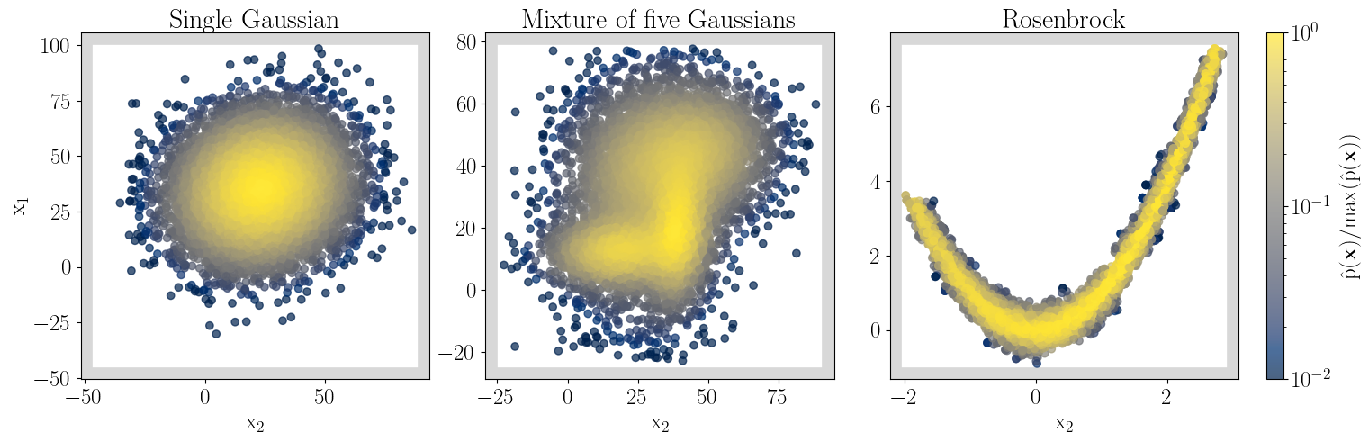
Figure 1: For each unnormalized posterior, we display $10^{4}$ posterior samples for the case $d=2$. For ease of comparison, the unnormalized posterior $\hat{\rm{p}}(\bf{x})$ is scaled by its maximum and shown in the common color bar. The shaded grey region represents the boundary of the rectangular prior.

III.3 Benchmarking

We evaluate the accuracy and efficiency of our flow-based evidence estimation in comparison to the importance nested sampling technique discussed in Ref. dynesty , using the code in Ref. dynesty_code , and to a $k$-nearest neighbors (hereon, referred to as $k$NN) technique Heavens:2017afc to estimate the evidence from MCMC chains of posterior samples using the recommended $k$ = 1 value. In the three panels of Figure 2, we show the comparison for the 2-dimensional unnormalized probability functions, with a flat rectangular prior. We use $10^{4}$ samples to evaluate the evidence using our method and the $k$NN technique. The nested sampling technique generates about $3\cdot 10^{4}$ samples for the evaluation. For $d=10$ and $d=15$, we evaluate the evidence using $10^{5}$ samples with our method and the $k$NN technique, whereas nested sampling uses between 5 to $9\cdot 10^{4}$ samples. We use the default values of the nested sampler's tolerance and live points, which are 0.01 and 500 respectively.

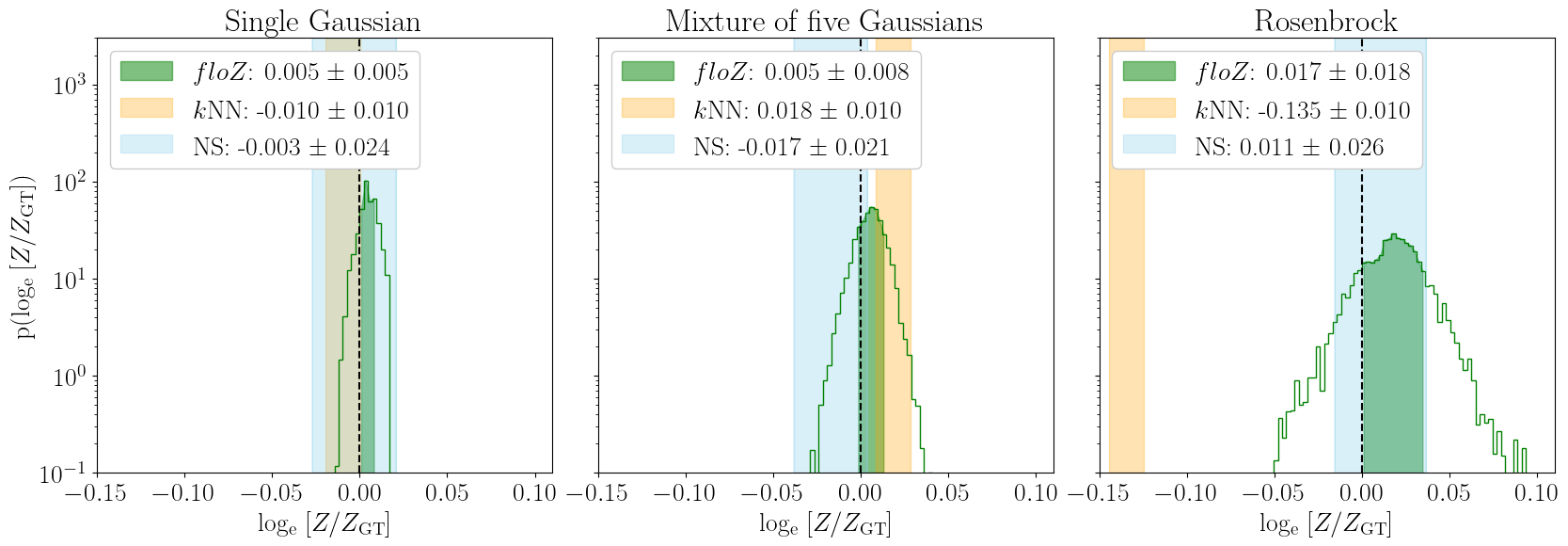
Figure 2: Evidence estimation in $d=2$ dimensions for (from left): multivariate Gaussian; finite multivariate Gaussian mixture; Rosenbrock. In all cases, floZ and $k$NN employ $10^{4}$ posterior samples. The true value, represented by the dashed line, has been rescaled to 0, and the shaded regions represent the 1-$\sigma$ uncertainty.

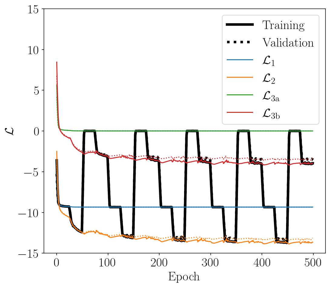
Figure 3: The evolution of the network's loss as a function of training epochs for the case of a 2-dimensional mixture of five Gaussians, illustrates the loss schedule. The four loss terms are shown in color, the total loss in thick/black, and the training (validation) losses are shown in solid (dotted) lines.

In Figure 3, we illustrate the behavior of the loss schedule for the Gaussian mixture case. The four individual loss terms are shown with different colors, the total loss in thick/black; training losses are depicted with continuous lines and validation losses with dotted ones. As described in Sec. II.4, we show that each loss term solely contributes to 20 epochs before linearly transitioning to the next term in 5 epochs. In a span of 500 epochs, the network is trained on 5 cycles of the loss terms.

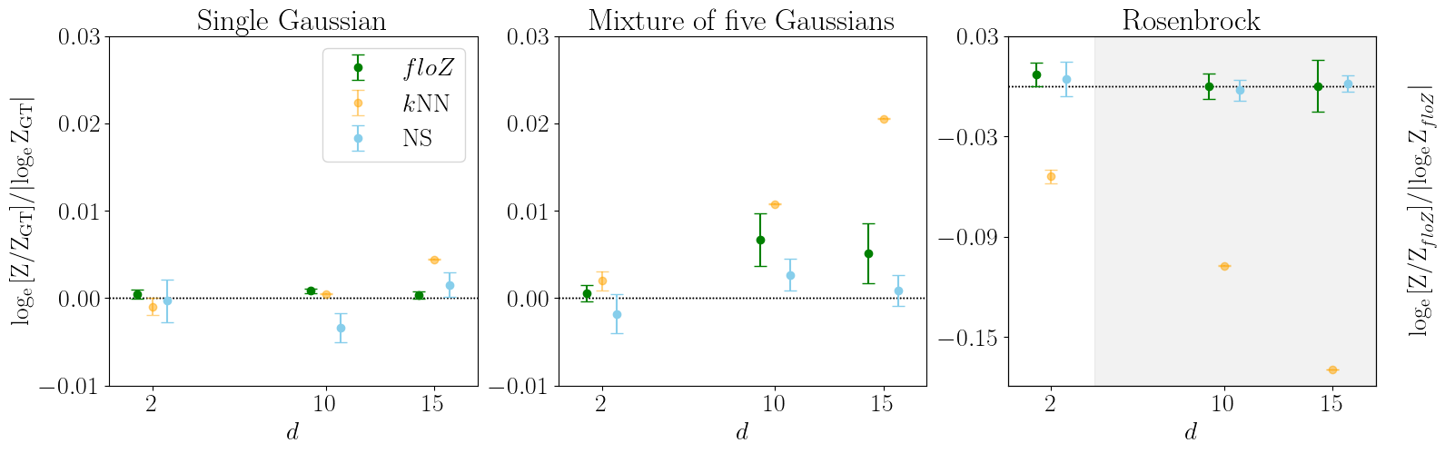
Figure 4: The relative error in the log evidence estimation for different distributions in each panel as a function of the dimensionality of parameter space, $d$. We compare the results of floZ and $k$NN using the same MCMC samples. We also show the evidence from nested sampling (labeled as NS). Since the ground truth for the higher-dimensional Rosenbrock likelihoods (grey-shaded region) is not numerically tractable, we compare the relative deviation from the floZ mean prediction (shown by the secondary y-axis).

Figure 4 compares the evidence evaluated by floZ, $k$NN, and nested sampling (labeled NS) techniques for the three distributions, each simulated in 2, 10, and 15 dimensions. The single Gaussian scenario has the simplest distribution and as a result, all methods perform well. However, with increasing complexity and higher dimensions, floZ and nested sampling are both more accurate than $k$NN.

The Rosenbrock likelihood provides an example with intractable evidence. The ground truth of the 2-dimensional case can be easily computed numerically, however, for higher dimensions, the numerical computation becomes too expensive. We show that for 10 and 15 dimensions, nested sampling and floZ are in agreement with each other within the estimated error bars.

It is difficult to fairly compare the computational effort required by floZ versus nested sampling, as the former takes as input posterior samples previously generated. Moreover, the efficiency of nested sampling depends on the details of the algorithm used, as well as on its settings (typically, the number of live samples and tolerance adopted). While we leave a more detailed study of actual scientific cases to future work, the $d=15$ results of this paper were obtained in less than 10 minutes on an A100 GPU.

IV Conclusions

In this work, we have introduced floZ, a novel method using normalizing flows for estimating the Bayesian evidence from posterior samples. Our approach computes the Bayesian evidence and its numerical uncertainty using pre-existing samples drawn from the target unnormalized posterior distribution, e.g. as obtained by standard MCMC methods.

Normalizing flows are built to map a complex target probability function (in our case, the unnormalized posterior distribution, given by the product of a likelihood and prior) into a simple probability distribution (e.g. a Gaussian). The transformation between the original variables and the latent ones is bijective and can be modeled with a neural network. Importantly for our method, the flows encode the volume of the real-space distribution, i.e. the Bayesian evidence. Our method hinges on this fact to compute the evidence from a set of posterior samples previously gathered by any suitable algorithm (e.g., MCMC), while at the same time minimizing the scatter of the estimates of the evidence across the samples by adding suitable terms to the custom loss function.

We have validated floZ against analytical benchmarks in parameter spaces of up to 15 dimensions: multivariate Gaussians, a finite multivariate Gaussian mixture, as well as the Rosenbrock distribution. Our method demonstrates performance comparable to nested sampling (which requires to be run ad hoc) and superior to a $k$-nearest neighbors method employed on the same posterior samples. We believe that floZ will add to the toolbox of astronomers and cosmologists seeking a fast, reliable method to compute the evidence from existing sets of posterior samples. floZ will be especially useful for cases where the likelihood is expensive and a full nested sampling run is difficult to achieve, while MCMC samples can be obtained more efficiently thanks to the ease of parallelization of many MCMC algorithms (such as Gibbs sampling). Pushing our approach to much larger parameter spaces is challenged by two limitations, both fundamentally stemming from the curse of dimensionality: first, obtaining posterior samples in high dimensions becomes typically more challenging (although some methods, like Gibbs sampling and Hamiltonian Monte Carlo, can show mild scaling with dimensionality in some favorable circumstances); second, training the flow in higher dimensions suffers from increasing inaccuracies. However, we note that we only need accurate densities in latent space near the peak (as opposed to into the tails of the distribution), which opens the door to potentially exploiting the existence of a well-defined `typical set' in high dimensions, a consequence of the concentration of measure phenomenon. We shall explore this idea further in a dedicated future paper.

Among the applications of floZ to gravitational-wave astronomy, it is worth mentioning the recent evidence for a stochastic signal reported by pulsar timing array experiments Antoniadis:2023ott ; Tarafdar:2022toa ; NANOGrav:2023gor ; Reardon:2023gzh ; Xu:2023wog . Within a Bayesian framework, interpreting the nature of this stochastic signal requires comparing different hypotheses and their evidences, which floZ could readily compute from the existing samples released by the experiments. Similarly, as another of the many possible applications, floZ could be used to investigate the statistical robustness of features/peaks that may be present in the mass function of the astrophysical black holes detected by the LIGO-Virgo-KAGRA collaboration KAGRA:2021duu .

Data availability: The floZ code and all the necessary files to reproduce the results in this paper will soon be made available.

- (1) R. Trotta, ``Bayes in the sky: Bayesian inference and model selection in cosmology,'' Contemporary Physics 49 no. 2, (Mar., 2008) 71–104, arXiv:0803.4089 [astro-ph].
- (2) J. Martin, C. Ringeval, R. Trotta, and V. Vennin, ``The Best Inflationary Models After Planck,'' JCAP 03 (2014) 039, arXiv:1312.3529 [astro-ph.CO].
- (3) A. F. Heavens and E. Sellentin, ``Objective Bayesian analysis of neutrino masses and hierarchy,'' JCAP 04 (2018) 047, arXiv:1802.09450 [astro-ph.CO].
- (4) A. Heavens, Y. Fantaye, E. Sellentin, H. Eggers, Z. Hosenie, S. Kroon, and A. Mootoovaloo, ``No Evidence for Extensions to the Standard Cosmological Model,'' Phys. Rev. Lett. 119 no. 10, (Sept., 2017) 101301, arXiv:1704.03467 [astro-ph.CO].
- (5) W. Del Pozzo, J. Veitch, and A. Vecchio, ``Testing General Relativity using Bayesian model selection: Applications to observations of gravitational waves from compact binary systems,'' Phys. Rev. D 83 (2011) 082002, arXiv:1101.1391 [gr-qc].
- (6) S. J. Vigeland and M. Vallisneri, ``Bayesian inference for pulsar timing models,'' Mon. Not. Roy. Astron. Soc. 440 no. 2, (2014) 1446–1457, arXiv:1310.2606 [astro-ph.IM].
- (7) A. Toubiana, K. W. K. Wong, S. Babak, E. Barausse, E. Berti, J. R. Gair, S. Marsat, and S. R. Taylor, ``Discriminating between different scenarios for the formation and evolution of massive black holes with LISA,'' Phys. Rev. D 104 (2021) 083027, arXiv:2106.13819 [gr-qc].
- (8) B. Lavie, J. M. Mendonça, C. Mordasini, M. Malik, M. Bonnefoy, B.-O. Demory, M. Oreshenko, S. L. Grimm, D. Ehrenreich, and K. Heng, ``Helios–retrieval: An open-source, nested sampling atmospheric retrieval code; application to the hr 8799 exoplanets and inferred constraints for planet formation,'' The Astronomical Journal 154 no. 3, (Aug., 2017) 91. http://dx.doi.org/10.3847/1538-3881/aa7ed8.
- (9) A. Lueber, D. Kitzmann, B. P. Bowler, A. J. Burgasser, and K. Heng, ``Retrieval Study of Brown Dwarfs across the L-T Sequence,'' ApJ 930 no. 2, (May, 2022) 136, arXiv:2204.01330 [astro-ph.EP].
- (10) J. Skilling, ``Nested Sampling,'' AIP Conference Proceedings 735 no. 1, (11, 2004) 395–405. https://doi.org/10.1063/1.1835238.
- (11) F. Feroz, M. P. Hobson, and M. Bridges, ``MULTINEST: an efficient and robust Bayesian inference tool for cosmology and particle physics,'' MNRAS 398 no. 4, (Oct., 2009) 1601–1614, arXiv:0809.3437 [astro-ph].
- (12) B. J. Brewer, L. B. Pártay, and G. Csányi, ``Diffusive Nested Sampling,'' arXiv e-prints (Dec., 2009) arXiv:0912.2380, arXiv:0912.2380 [stat.CO].
- (13) E. Higson, W. Handley, M. Hobson, and A. Lasenby, ``Dynamic nested sampling: an improved algorithm for parameter estimation and evidence calculation,'' Statistics and Computing 29 no. 5, (Sept., 2019) 891–913, arXiv:1704.03459 [stat.CO].
- (14) A. Moss, ``Accelerated Bayesian inference using deep learning,'' Mon. Not. Roy. Astron. Soc. 496 no. 1, (2020) 328–338, arXiv:1903.10860 [astro-ph.CO].
- (15) J. Buchner, ``Nested Sampling Methods,'' Statistics Surveys 17 (Jan., 2023) 169–215, arXiv:2101.09675 [stat.CO].
- (16) W. J. Handley, M. P. Hobson, and A. N. Lasenby, ``POLYCHORD: next-generation nested sampling,'' MNRAS 453 no. 4, (Nov., 2015) 4384–4398, arXiv:1506.00171 [astro-ph.IM].
- (17) X. Cai, J. D. McEwen, and M. Pereyra, ``Proximal nested sampling for high-dimensional Bayesian model selection,'' arXiv e-prints (June, 2021) arXiv:2106.03646, arXiv:2106.03646 [stat.ME].
- (18) E. Ruli, N. Sartori, and L. Ventura, ``Improved Laplace approximation for marginal likelihoods,'' Electronic Journal of Statistics 10 no. 2, (2016) 3986 – 4009. https://doi.org/10.1214/16-EJS1218.
- (19) R. Trotta, ``Applications of Bayesian model selection to cosmological parameters,'' Mon. Not. Roy. Astron. Soc. 378 (2007) 72–82, arXiv:astro-ph/0504022.
- (20) P. M. Goggans and Y. Chi, ``Using Thermodynamic Integration to Calculate the Posterior Probability in Bayesian Model Selection Problems,'' AIP Conference Proceedings 707 no. 1, (04, 2004) 59–66. https://doi.org/10.1063/1.1751356.
- (21) K. Karchev, R. Trotta, and C. Weniger, ``SimSIMS: Simulation-based Supernova Ia Model Selection with thousands of latent variables,'' arXiv e-prints (Nov., 2023) arXiv:2311.15650, arXiv:2311.15650 [astro-ph.CO].
- (22) N. Jeffrey and B. D. Wandelt, ``Evidence Networks: simple losses for fast, amortized, neural Bayesian model comparison,'' Mach. Learn. Sci. Tech. 5 no. 1, (2024) 015008, arXiv:2305.11241 [cs.LG].
- (23) S. T. Radev, M. D'Alessandro, U. K. Mertens, A. Voss, U. Köthe, and P.-C. Bürkner, ``Amortized Bayesian model comparison with evidential deep learning,'' arXiv e-prints (Apr., 2020) arXiv:2004.10629, arXiv:2004.10629 [stat.ML].
- (24) A. Heavens, Y. Fantaye, A. Mootoovaloo, H. Eggers, Z. Hosenie, S. Kroon, and E. Sellentin, ``Marginal Likelihoods from Monte Carlo Markov Chains,'' arXiv:1704.03472 [stat.CO].
- (25) J. D. McEwen, C. G. R. Wallis, M. A. Price, and A. Spurio Mancini, ``Machine learning assisted Bayesian model comparison: learnt harmonic mean estimator,'' arXiv e-prints (Nov., 2021) arXiv:2111.12720, arXiv:2111.12720 [stat.ME].
- (26) E. Tabak and E. Vanden-Eijnden, ``Density estimation by dual ascent of the log-likelihood,'' Communications in Mathematical Sciences 8 no. 1, (2010) 217–233.
- (27) E. Tabak and C. Turner, ``A family of nonparametric density estimation algorithms,'' Communications on Pure and Applied Mathematics 66 no. 2, (Feb., 2013) 145–164.
- (28) J. P. Agnelli, M. Cadeiras, E. G. Tabak, C. V. Turner, and E. Vanden-Eijnden, ``Clustering and classification through normalizing flows in feature space,'' Multiscale Modeling & Simulation 8 no. 5, (2010) 1784–1802, https://doi.org/10.1137/100783522. https://doi.org/10.1137/100783522.
- (29) O. Rippel and R. P. Adams, ``High-dimensional probability estimation with deep density models,'' 2013.
- (30) P. Laurence, R. Pignol, and E. Tabak, Constrained density estimation, pp. 259–284. Springer-Verlag, 2014.
- (31) D. J. Rezende and S. Mohamed, ``Variational inference with normalizing flows,'' in Proceedings of the 32nd International Conference on International Conference on Machine Learning, vol. 37 of ICML'15, p. 1530–1538. JMLR.org, 2015.
- (32) S. R. Green, C. Simpson, and J. Gair, ``Gravitational-wave parameter estimation with autoregressive neural network flows,'' Phys. Rev. D 102 no. 10, (2020) 104057, arXiv:2002.07656 [astro-ph.IM].
- (33) S. R. Green and J. Gair, ``Complete parameter inference for GW150914 using deep learning,'' Mach. Learn. Sci. Tech. 2 no. 3, (2021) 03LT01, arXiv:2008.03312 [astro-ph.IM].
- (34) M. Dax, S. R. Green, J. Gair, J. H. Macke, A. Buonanno, and B. Schölkopf, ``Real-Time Gravitational Wave Science with Neural Posterior Estimation,'' Phys. Rev. Lett. 127 no. 24, (2021) 241103, arXiv:2106.12594 [gr-qc].
- (35) M. Dax, S. R. Green, J. Gair, M. Deistler, B. Schölkopf, and J. H. Macke, ``Group equivariant neural posterior estimation,'' arXiv:2111.13139 [cs.LG].
- (36) M. Dax, S. R. Green, J. Gair, M. Pürrer, J. Wildberger, J. H. Macke, A. Buonanno, and B. Schölkopf, ``Neural Importance Sampling for Rapid and Reliable Gravitational-Wave Inference,'' Phys. Rev. Lett. 130 no. 17, (Apr., 2023) 171403, arXiv:2210.05686 [gr-qc].
- (37) J. Wildberger, M. Dax, S. R. Green, J. Gair, M. Pürrer, J. H. Macke, A. Buonanno, and B. Schölkopf, ``Adapting to noise distribution shifts in flow-based gravitational-wave inference,'' arXiv:2211.08801 [gr-qc].
- (38) U. Bhardwaj, J. Alvey, B. K. Miller, S. Nissanke, and C. Weniger, ``Peregrine: Sequential simulation-based inference for gravitational wave signals,'' arXiv:2304.02035 [gr-qc].
- (39) M. Crisostomi, K. Dey, E. Barausse, and R. Trotta, ``Neural posterior estimation with guaranteed exact coverage: The ringdown of GW150914,'' Phys. Rev. D 108 no. 4, (2023) 044029, arXiv:2305.18528 [gr-qc].
- (40) K. Leyde, S. R. Green, A. Toubiana, and J. Gair, ``Gravitational wave populations and cosmology with neural posterior estimation,'' Phys. Rev. D 109 no. 6, (2024) 064056, arXiv:2311.12093 [gr-qc].
- (41) D. Shih, M. Freytsis, S. R. Taylor, J. A. Dror, and N. Smyth, ``Fast Parameter Inference on Pulsar Timing Arrays with Normalizing Flows,'' arXiv:2310.12209 [astro-ph.IM].
- (42) S. Koposov, J. Speagle, K. Barbary, G. Ashton, E. Bennett, J. Buchner, C. Scheffler, B. Cook, C. Talbot, J. Guillochon, P. Cubillos, A. A. Ramos, B. Johnson, D. Lang, Ilya, M. Dartiailh, A. Nitz, A. McCluskey, and A. Archibald, ``joshspeagle/dynesty: v2.1.3,'' Oct., 2023. https://doi.org/10.5281/zenodo.8408702.
- (43) C. Villani, Topics in optimal transportation. Graduate studies in mathematics. American mathematical society, Providence, Rhode Island, 2003.
- (44) V. I. Bogachev, A. V. Kolesnikov, and K. V. Medvedev, ``Triangular transformations of measures,'' Sbornik: Mathematics 196 no. 3, (Apr, 2005) 309. https://dx.doi.org/10.1070/SM2005v196n03ABEH000882.
- (45) K. Medvedev, ``Certain properties of triangular transformations of measures,'' Theory of Stochastic Processes 1 (01, 2008) .
- (46) G. Papamakarios, T. Pavlakou, and I. Murray, ``Masked autoregressive flow for density estimation,'' Advances in neural information processing systems 30 (2017) .
- (47) D. P. Kingma and J. Ba, ``Adam: A method for stochastic optimization,'' CoRR abs/1412.6980 (Dec., 2014) arXiv:1412.6980, arXiv:1412.6980 [cs.LG].
- (48) T. J. DiCiccio, R. E. Kass, A. Raftery, and L. Wasserman, ``Computing bayes factors by combining simulation and asymptotic approximations,'' Journal of the American Statistical Association 92 no. 439, (1997) 903–915. http://www.jstor.org/stable/2965554.
- (49) H. Rosenbrock, ``An automatic method for finding the greatest or least value of a function,'' Comput. J. 3 (1960) 175–184. https://api.semanticscholar.org/CorpusID:62755334.
- (50) J. Goodman and J. Weare, ``Ensemble samplers with affine invariance,'' Communications in Applied Mathematics and Computational Science 5 no. 1, (Jan., 2010) 65–80.
- (51) F. Pagani, M. Wiegand, and S. Nadarajah, ``An n‐dimensional rosenbrock distribution for mcmc testing,'' Scandinavian Journal of Statistics 49 (04, 2021) .
- (52) J. S. Speagle, ``DYNESTY: a dynamic nested sampling package for estimating Bayesian posteriors and evidences,'' MNRAS 493 no. 3, (Apr., 2020) 3132–3158, arXiv:1904.02180 [astro-ph.IM].
- (53) EPTA, InPTA: Collaboration, J. Antoniadis et al., ``The second data release from the European Pulsar Timing Array - III. Search for gravitational wave signals,'' Astron. Astrophys. 678 (2023) A50, arXiv:2306.16214 [astro-ph.HE].
- (54) P. Tarafdar et al., ``The Indian Pulsar Timing Array: First data release,'' Publ. Astron. Soc. Austral. 39 (2022) e053, arXiv:2206.09289 [astro-ph.IM].
- (55) NANOGrav Collaboration, G. Agazie et al., ``The NANOGrav 15 yr Data Set: Evidence for a Gravitational-wave Background,'' Astrophys. J. Lett. 951 no. 1, (2023) L8, arXiv:2306.16213 [astro-ph.HE].
- (56) D. J. Reardon et al., ``Search for an Isotropic Gravitational-wave Background with the Parkes Pulsar Timing Array,'' Astrophys. J. Lett. 951 no. 1, (2023) L6, arXiv:2306.16215 [astro-ph.HE].
- (57) H. Xu et al., ``Searching for the Nano-Hertz Stochastic Gravitational Wave Background with the Chinese Pulsar Timing Array Data Release I,'' Res. Astron. Astrophys. 23 no. 7, (2023) 075024, arXiv:2306.16216 [astro-ph.HE].
- (58) KAGRA, VIRGO, LIGO Scientific Collaboration, R. Abbott et al., ``Population of Merging Compact Binaries Inferred Using Gravitational Waves through GWTC-3,'' Phys. Rev. X 13 no. 1, (2023) 011048, arXiv:2111.03634 [astro-ph.HE].