\mytite

Lingxiao Li    Raaz Dwivedi    Lester Mackey

Debiased Distribution Compression

Lingxiao Li    Raaz Dwivedi    Lester Mackey
Abstract

Modern compression methods can summarize a target distribution $\mathbb{P}$ more succinctly than i.i.d. sampling but require access to a low-bias input sequence like a Markov chain converging quickly to $\mathbb{P}$. We introduce a new suite of compression methods suitable for compression with biased input sequences. Given $n$ points targeting the wrong distribution and quadratic time, Stein Kernel Thinning (SKT) returns $\sqrt{n}$ equal-weighted points with $\widetilde{O}(n^{-1/2})$ maximum mean discrepancy (MMD) to $\mathbb{P}$. For larger-scale compression tasks, Low-rank SKT achieves the same feat in sub-quadratic time using an adaptive low-rank debiasing procedure that may be of independent interest. For downstream tasks that support simplex or constant-preserving weights, Stein Recombination and Stein Cholesky achieve even greater parsimony, matching the guarantees of SKT with as few as $\operatorname{poly-log}(n)$ weighted points. Underlying these advances are new guarantees for the quality of simplex-weighted coresets, the spectral decay of kernel matrices, and the covering numbers of Stein kernel Hilbert spaces. In our experiments, our techniques provide succinct and accurate posterior summaries while overcoming biases due to burn-in, approximate Markov chain Monte Carlo, and tempering.

Machine Learning, ICML

\etoctocstyle

1Table of contents \etocdepthtag.tocmtchapter \etocsettagdepthmtchaptersection

1 Introduction

Table 1: Methods for debiased distribution compression. For each method, we report the smallest coreset size $m$ and running time, up to logarithmic factors, sufficient to guarantee $\widetilde{O}(n^{-1/2})$ $\operatorname{MMD}_{{{\bm{k}}_{\mathbb{P}}}}$ to $\mathbb{P}$ given a LogGrowth kernel ${{\bm{k}}_{\mathbb{P}}}$ and $n$ slow-growing input points $\mathcal{S}_{n}=(x_{i})_{i=1}^{n}$ from a fast-mixing Markov chain targeting $\mathbb{Q}$ with tails no lighter than $\mathbb{P}$ (see Thms. 1 and 3). For generic slow-growing $\mathcal{S}_{n}$, identical guarantees hold for excess $\operatorname{MMD}_{{{\bm{k}}_{\mathbb{P}}}}$ (8) relative to the best simplex reweighting of $\mathcal{S}_{n}$.
Method Compression Type
Coreset Size $\bm{m}$
Runtime Source
Stein Thinning (Riabiz et al., 2022) equal-weighted ${\color[rgb]{1,0,0}{n}}$ $d_{{{\bm{k}}_{\mathbb{P}}}}n^{2}$ Sec. D.1
Stein Kernel Thinning  $\begin{cases}\textup{Greedy}\\ \textup{Low-rank}\end{cases}$
(Alg. 1)
(Alg. 3)
equal-weighted ${\color[rgb]{0,0,1}{\sqrt{n}}}$
$d_{{{\bm{k}}_{\mathbb{P}}}}n^{2}$
$\ \ \,d_{{{\bm{k}}_{\mathbb{P}}}}n^{1.5}$
Thm. 3
Thm. 5
Stein Recombination  $\begin{cases}\textup{Greedy}\\ \textup{Low-rank}\end{cases}$ (Alg. 5) simplex-weighted ${\color[rgb]{0,0,1}{\operatorname{poly-log}(n)}}$
$d_{{{\bm{k}}_{\mathbb{P}}}}n^{2}$
$\ \ \,d_{{{\bm{k}}_{\mathbb{P}}}}n+n^{1.5}$
Thm. 6
Stein Cholesky  $\begin{cases}\textup{Greedy}\\ \textup{Low-rank}\end{cases}$ (Alg. 7) constant-preserving ${\color[rgb]{0,0,1}{\operatorname{poly-log}(n)}}$
$d_{{{\bm{k}}_{\mathbb{P}}}}n^{2}$
$\ \ \,d_{{{\bm{k}}_{\mathbb{P}}}}n+n^{1.5}$
Thm. 7

Distribution compression is the problem of summarizing a target probability distribution $\mathbb{P}$ with a small set of representative points. Such compact summaries are particularly valuable for tasks that incur substantial downstream computation costs per summary point, like organ and tissue modeling in which each simulation consumes thousands of CPU hours (Niederer et al., 2011).

Remarkably, modern compression methods can summarize a distribution more succinctly than i.i.d. sampling. For example, kernel thinning (KT) (Dwivedi and Mackey, 2021, 2022), Compress++ (Shetty et al., 2022), recombination (Hayakawa et al., 2023), and randomly pivoted Cholesky (Epperly and Moreno, 2024) all provide $\widetilde{O}(1/m)$ approximation error using $m$ points, a significant improvement over the $\Omega(1/\sqrt{m})$ approximation provided by i.i.d. sampling from $\mathbb{P}$. However, each of these constructions relies on access to an accurate input sequence, like an i.i.d. sample from $\mathbb{P}$ or a Markov chain converging quickly to $\mathbb{P}$.

Much more commonly, one only has access to $n$ biased sample points approximating a wrong distribution $\mathbb{Q}$. Such biases are a common occurrence in Markov chain Monte Carlo (MCMC)-based inference due to tempering (where one targets a less peaked and more dispersed distribution to achieve faster convergence, Gramacy et al., 2010), burn-in (where the initial state of a Markov chain biases the distribution of chain iterates, Cowles and Carlin, 1996), or approximate MCMC (where one runs a cheaper approximate Markov chain to avoid the prohibitive costs of an exact MCMC algorithm, e.g., Ahn et al., 2012). The Stein thinning (ST) method of Riabiz et al. (2022) was developed to provide accurate compression even when the input sample sequence provides a poor approximation to the target. ST operates by greedily thinning the input sample to minimize the maximum mean discrepancy (MMD, Gretton et al., 2012) to $\mathbb{P}$. However, ST is only known to provide an $O(1/\sqrt{m})$ approximation to $\mathbb{P}$; this guarantee is no better than that of i.i.d. sampling and a far cry from the $\widetilde{O}(1/m)$ error achieved with unbiased coreset constructions.

In this work, we address this deficit by developing new, efficient coreset constructions that provably yield better-than-i.i.d. error even when the input sample is biased. For $\mathbb{P}$ on $\mathbb{R}^{d}$, our primary contributions are fourfold and summarized in Tab. 1. First, for the task of equal-weighted compression, we introduce Stein Kernel Thinning (SKT, Alg. 1), a strategy that combines the greedy bias correction properties of ST with the unbiased compression of KT to produce $\sqrt{n}$ summary points with error $\widetilde{O}(n^{-1/2})$ in $O(n^{2})$ time. In contrast, ST would require $\Omega(n)$ points to guarantee this error. Second, for larger-scale compression problems, we propose Low-rank SKT (Alg. 3), a strategy that combines the scalable summarization of Compress++ with a new low-rank debiasing procedure (Alg. 2) to match the SKT guarantees in sub-quadratic $o(n^{2})$ time.

Third, for the task of simplex-weighted compression, in which summary points are accompanied by weights in the simplex, we propose greedy and low-rank Stein Recombination (Alg. 5) constructions that match the guarantees of SKT with as few as $\operatorname{poly-log}(n)$ points. Finally, for the task of constant-preserving compression, in which summary points are accompanied by real-valued weights summing to $1$, we introduce greedy and low-rank Stein Cholesky (Alg. 7) constructions that again match the guarantees of SKT using as few as $\operatorname{poly-log}(n)$ points.

Underlying these advances are new guarantees for the quality of simplex-weighted coresets (Thms. 1 and 2), the spectral decay of kernel matrices (Cor. B.1), and the covering numbers of Stein kernel Hilbert spaces (Prop. 1) that may be of independent interest. In Sec. 5, we employ our new procedures to produce compact summaries of complex target distributions given input points biased by burn-in, approximate MCMC, or tempering.

Notation   We assume Borel-measurable sets and functions and define $[n]\triangleq\{1,\ldots,n\}$, $\Delta_{n-1}\triangleq\{w\in\mathbb{R}^{n}:w\geq 0,\bm{1}^{\top}w=1\}$, $\|{x}\|_{0}\triangleq\absolutevalue{\{i:x_{i}\neq 0\}}$, and $\|{x}\|_{p}^{p}\triangleq\sum_{i}|x_{i}|^{p}$ for $x\in\mathbb{R}^{d}$ and $p\geq 1$. For $x\in\mathbb{R}^{d}$, $\delta_{x}$ denotes the delta measure at $x$. We let ${\mathcal{H}_{{\bm{k}}}}$ denote the reproducing kernel Hilbert space (RKHS) of a kernel ${\bm{k}}:\mathbb{R}^{d}\times\mathbb{R}^{d}\to\mathbb{R}$ (Aronszajn, 1950) and $\left\|{f}\right\|_{{\bm{k}}}$ denote the RKHS norm of $f\in{\mathcal{H}_{{\bm{k}}}}$. For a measure $\mu$ and separately $\mu$-integrable ${\bm{k}}$ and $f$, we write $\mu f\!\triangleq\!\int f(x)\differential\mu(x)$ and $\mu{\bm{k}}(x)\!\triangleq\!\int{\bm{k}}(x,y)\differential\mu(y)$. The divergence of a differentiable matrix-valued function $A$ is $(\nabla_{x}\cdot A(x))_{j}=\sum_{i}\partial_{x_{i}}A_{ij}(x)$. For random variables $(X_{n})_{n\in\mathbb{N}}$, we say $X_{n}\!=\!O(f(n,\delta))$ holds with probability $\geq 1\!-\!\delta$ if $\Pr(X_{n}\!\leq\!Cf(n,\delta))\geq 1\!-\!\delta$ for a constant $C$ independent of $(n,\delta)$ and all $n$ sufficiently large. When using this notation, we view all algorithm parameters except $\delta$ as functions of $n$. For $A\!\in\!\mathbb{R}^{n\times n}$ and $v\in\mathbb{R}^{n}$, $\operatorname{diag}(A)$ and $\operatorname{diag}(v)$ are $n\times n$ diagonal matrices with $A_{ii}$ and $v_{i}$ respectively as the $i$-th diagonal entry.

2 Debiased Distribution Compression

Throughout, we aim to summarize a fixed target distribution $\mathbb{P}$ on $\mathbb{R}^{d}$ using a sequence $\mathcal{S}_{n}\triangleq(x_{i})_{i=1}^{n}$ of potentially biased candidate points in $\mathbb{R}^{d}$.111Our coreset constructions will in fact apply to any sample space, but our analysis will focus on $\mathbb{R}^{d}$. Correcting for unknown biases in $\mathcal{S}_{n}$ requires some auxiliary knowledge of $\mathbb{P}$. For us, this knowledge comes in the form of a kernel function ${{\bm{k}}_{\mathbb{P}}}$ with known expectation under $\mathbb{P}$. Without loss of generality, we can take this kernel mean to be identically zero.222For $\mathbb{P}{{\bm{k}}_{\mathbb{P}}}\not\equiv 0$, the kernel ${{\bm{k}}_{\mathbb{P}}}^{\prime}(x,y)={{\bm{k}}_{\mathbb{P}}}(x,y)-\mathbb{P}{{\bm{k}}_{\mathbb{P}}}(x)-\mathbb{P}{{\bm{k}}_{\mathbb{P}}}(y)+\mathbb{P}\mathbb{P}{{\bm{k}}_{\mathbb{P}}}$ satisfies $\mathbb{P}{{\bm{k}}_{\mathbb{P}}}^{\prime}\equiv 0$ and $\operatorname{MMD}_{{{\bm{k}}_{\mathbb{P}}}^{\prime}}=\operatorname{MMD}_{{{\bm{k}}_{\mathbb{P}}}}$.

Assumption 1 (Mean-zero kernel).

For some $\mathfrak{p}\geq 1/2$, $\mathbb{E}_{x\sim\mathbb{P}}[{{\bm{k}}_{\mathbb{P}}}(x,x)^{\mathfrak{p}}]<\infty$ and $\mathbb{P}{{\bm{k}}_{\mathbb{P}}}\equiv 0$.

Given a target compression size $m$, our goal is to output an weight vector $w\in\mathbb{R}^{n}$ with $\left\|{w}\right\|_{0}\leq m$, $\bm{1}_{n}^{\top}w=1$, and $o(m^{-1/2})$ (better-than-i.i.d.) maximum mean discrepancy (MMD) to $\mathbb{P}$:

$\textstyle\operatorname{MMD}_{{{\bm{k}}_{\mathbb{P}}}}(\sum_{i=1}^{n}\!w_{i}\mathbf{\delta}_{x_{i}},\mathbb{P})\triangleq\sqrt{\sum_{i,j=1}^{n}\!w_{i}w_{j}{{\bm{k}}_{\mathbb{P}}}(x_{i},x_{j})}.$ (1)

We consider three standard compression tasks with $\left\|{w}\right\|_{0}\leq m$. In equal-weighted compression one selects $m$ possibly repeated points from $\mathcal{S}_{n}$ and assigns each a weight of $\frac{1}{m}$; because of repeats, the induced weight vector over $\mathcal{S}_{n}$ satisfies $w\in\Delta_{n-1}\cap(\frac{\mathbb{N}_{0}}{m})^{n}$. In simplex-weighted compression we allow any $w\in\Delta_{n-1}$, and in constant-preserving compression we simply enforce $\bm{1}_{n}^{\top}w=1$.

When making big O statements, we will treat $\mathcal{S}_{n}$ as the prefix of an infinite sequence $\mathcal{S}_{\infty}\triangleq(x_{i})_{i\in\mathbb{N}}$. We also write ${{\bm{k}}_{\mathbb{P}}}(\mathcal{S}_{n}[\mathtt{J}],\mathcal{S}_{n}[\mathtt{J}])\triangleq[{{\bm{k}}_{\mathbb{P}}}(x_{i},x_{j})]_{i,j\in\mathtt{J}}$ for the principal kernel submatrix with indices $\mathtt{J}\subseteq[n]$.

2.1 Kernel assumptions

Many practical Stein kernel constructions are available for generating mean-zero kernels for a target $\mathbb{P}$ (Chwialkowski et al., 2016; Liu et al., 2016; Gorham and Mackey, 2017; Gorham et al., 2019; Barp et al., 2019; Yang et al., 2018; Afzali and Muthukumarana, 2023). We will use the most prominent of these Stein kernels as a running example:

Definition 1 (Stein kernel).

Given a differentiable base kernel ${\bm{k}}$ and a symmetric positive semidefinite matrix $M$, the Stein kernel ${{\bm{k}}_{p}}:\mathbb{R}^{d}\times\mathbb{R}^{d}\to\mathbb{R}$ for $\mathbb{P}$ with positive differentiable Lebesgue density $p$ is defined as

$\textstyle{{\bm{k}}_{p}}(x,y)\triangleq\frac{1}{p(x)p(y)}{\nabla_{x}\cdot\nabla_{y}\cdot(p(x)M{\bm{k}}(x,y)p(y))}.$ (2)

While our algorithms apply to any mean zero kernel, our guarantees adapt to the underlying smoothness of the kernels. Our next definition and assumption make this precise.

Definition 2 (Covering number).

For a kernel ${\bm{k}}:\mathbb{R}^{d}\times\mathbb{R}^{d}\to\mathbb{R}$ with $\mathcal{B}_{{\bm{k}}}\triangleq\{f\in{\mathcal{H}_{{\bm{k}}}}:\left\|{f}\right\|_{{\bm{k}}}\leq 1\}$, a set $A\subset\mathbb{R}^{d}$, and $\varepsilon>0$, the covering number $\mathcal{N}_{{\bm{k}}}(A,\varepsilon)$ is the minimum cardinality of all sets $\mathcal{C}\subset\mathcal{B}_{{\bm{k}}}$ satisfying

$\textstyle\mathcal{B}_{{\bm{k}}}\subset\bigcup_{h\in\mathcal{C}}\{g\in\mathcal{B}_{{\bm{k}}}:\sup_{x\in A}\absolutevalue{h(x)-g(x)}\leq\varepsilon\}.$ (3)
Assumption ($\bm{{\alpha},{\beta}}$)-kernel.

For some $\mathfrak{C}_{d}>0$, all $r>0$ and $\varepsilon\in(0,1)$, and $\mathcal{B}_{2}(r)\triangleq\{x\in\mathbb{R}^{d}:\left\|{x}\right\|_{2}\leq r\}$, a kernel ${\bm{k}}$ is either PolyGrowth(α,β)PolyGrowth𝛼𝛽\hyperref@@ii[assum:kernel_growth]{\color[rgb]{0,0,0}{\textsc{PolyGrowth}}}({\alpha},{\beta}), i.e.,

$\textstyle\log\mathcal{N}_{{\bm{k}}}(\mathcal{B}_{2}(r),\varepsilon)\leq\mathfrak{C}_{d}(1/\varepsilon)^{{\alpha}}(r+1)^{{\beta}},$ (4)

with $\alpha<2$ or LogGrowth(α,β)LogGrowth𝛼𝛽\hyperref@@ii[assum:kernel_growth]{\color[rgb]{0,0,0}{\textsc{LogGrowth}}}({\alpha},{\beta}), i.e.,

$\textstyle\log\mathcal{N}_{{\bm{k}}}(\mathcal{B}_{2}(r),\varepsilon)\leq\mathfrak{C}_{d}\log(e/\varepsilon)^{{\alpha}}(r+1)^{{\beta}}.$ (5)

In Cor. B.1 we show that the eigenvalues of kernel matrices with PolyGrowth and LogGrowth kernels have polynomial and exponential decay respectively. Dwivedi and Mackey (2022, Prop. 2) showed that all sufficiently differentiable kernels satisfy the PolyGrowth condition and that bounded radially analytic kernels are LogGrowth. Our next result, proved in Sec. B.2, shows that a Stein kernel ${{\bm{k}}_{p}}$ can inherit the growth properties of its base kernel even if ${{\bm{k}}_{p}}$ is itself unbounded and non-smooth.

Proposition 1 (Stein kernel growth rates).

A Stein kernel ${{\bm{k}}_{p}}$ with $\sup_{\|{x}\|_{2}\leq r}\|{\nabla\log p(x)}\|_{2}=O(r^{d_{\ell}})$ for $d_{\ell}\geq 0$ is

  1. (a)

    LogGrowth(d+1,2d+δ)LogGrowth𝑑12𝑑𝛿\hyperref@@ii[assum:kernel_growth]{\color[rgb]{0,0,0}{\textsc{LogGrowth}}}(d+1,2d+\delta) for any $\delta>0$ if the base kernel ${\bm{k}}$ is radially analytic (Def. B.3) and

  2. (b)

    PolyGrowth(ds1,(1+ds)d)PolyGrowth𝑑𝑠11subscript𝑑𝑠𝑑\hyperref@@ii[assum:kernel_growth]{\color[rgb]{0,0,0}{\textsc{PolyGrowth}}}(\frac{d}{s-1},(1+\frac{d_{\ell}}{s})d) if the base kernel ${\bm{k}}$ is $s$-times continuously differentiable (Def. B.2) for $s\!>\!1$.

Notably, the popular Gaussian (Ex. B.1) and inverse multiquadric (Ex. B.2) base kernels satisfy the LogGrowth preconditions, while Matérn, B-spline, sinc, sech, and Wendland’s compactly supported kernels satisfy the PolyGrowth precondition (Dwivedi and Mackey, 2022, Prop. 3). To our knowledge, Prop. 1 provides the first covering number bounds and eigenvalue decay rates for the (typically unbounded) Stein kernels ${{\bm{k}}_{p}}$.

2.2 Input point desiderata

Our primary desideratum for the input points is that they can be debiased into an accurate estimate of $\mathbb{P}$. Indeed, our high-level strategy for debiased compression is to first use ${{\bm{k}}_{\mathbb{P}}}$ to debias the input points into a more accurate approximation of $\mathbb{P}$ and then compress that approximation into a more succinct representation. Fortunately, even when the input $\mathcal{S}_{n}$ targets a distribution $\mathbb{Q}\neq\mathbb{P}$, effective debiasing is often achievable via simplex reweighting, i.e., by solving the convex optimization problem

$\textstyle{w_{\textsc{OPT}}}\in\arg\min_{w\in\Delta_{n-1}}\sum_{i,j=1}^{n}w_{i}w_{j}{{\bm{k}}_{\mathbb{P}}}(x_{i},x_{j})$ (6)
$\textstyle\text{with }\,\operatorname{MMD}_{\textsc{OPT}}\triangleq\operatorname{MMD}_{{{\bm{k}}_{\mathbb{P}}}}(\sum_{i=1}^{n}\!{w_{\textsc{OPT}}}_{i}\mathbf{\delta}_{x_{i}},\mathbb{P}).$ (7)

For example, Hodgkinson et al. (2020, Thm. 1b) showed that simplex reweighting can correct for biases due to off-target i.i.d. or MCMC sampling. Our next result (proved in Sec. C.2) significantly relaxes their conditions.

Theorem 1 (Debiasing via simplex reweighting).

Consider a kernel ${{\bm{k}}_{\mathbb{P}}}$ satisfying Assum. 1 with ${\mathcal{H}_{{{\bm{k}}_{\mathbb{P}}}}}$ separable, and suppose $(x_{i})_{i=1}^{\infty}$ are the iterates of a homogeneous $\phi$-irreducible geometrically ergodic Markov chain (Gallegos-Herrada et al., 2023, Thm. 1) with stationary distribution $\mathbb{Q}$ and initial distribution absolutely continuous with respect to $\mathbb{P}$. If $\mathbb{E}_{x\sim\mathbb{P}}[\frac{\differential\mathbb{P}}{\differential\mathbb{Q}}(x)^{2\mathfrak{q}-1}{{\bm{k}}_{\mathbb{P}}}(x,x)^{\mathfrak{q}}]<\infty$ for some $\mathfrak{q}>1$ then $\operatorname{MMD}_{\textsc{OPT}}=O(n^{-1/2})$ in probability.

Remark 1.

${\mathcal{H}_{{{\bm{k}}_{\mathbb{P}}}}}$ is separable whenever ${{\bm{k}}_{\mathbb{P}}}$ is continuous (Steinwart and Christmann, 2008, Lem. 4.33).

Since $n$ points sampled i.i.d. from $\mathbb{P}$ have $\Theta(n^{-1/2})$ root mean squared MMD (see Prop. C.1), Thm. 1 shows that a debiased off-target sample can be as accurate as a direct sample from $\mathbb{P}$. Moreover, Thm. 1 applies to many practical examples. The simplest example of a geometrically ergodic chain is i.i.d. sampling from $\mathbb{Q}$, but geometric ergodicity has also been established for a variety of popular Markov chains including random walk Metropolis (Roberts and Tweedie, 1996, Thm. 3.2), independent Metropolis-Hastings (Atchadé and Perron, 2007, Thm. 2.2), the unadjusted Langevin algorithm (Durmus and Moulines, 2017, Prop. 8), the Metropolis-adjusted Langevin algorithm (Durmus and Moulines, 2022, Thm. 1), Hamiltonian Monte Carlo (Durmus et al., 2020, Thm. 10 and Thm. 11), stochastic gradient Langevin dynamics (Li et al., 2023, Thm. 2.1), and the Gibbs sampler (Johnson, 2009). Moreover, for $\mathbb{Q}$ absolutely continuous with respect to $\mathbb{P}$, the importance weight $\frac{\differential\mathbb{P}}{\differential\mathbb{Q}}$ is typically bounded or slowly growing when the tails of $\mathbb{Q}$ are not much lighter than those of $\mathbb{P}$.

Remarkably, under more stringent conditions, Thm. 2 (proved in Sec. C.3) shows that simplex reweighting can decrease MMD to $\mathbb{P}$ at an even-faster-than-i.i.d. rate.

Theorem 2 (Better-than-i.i.d. debiasing via simplex reweighting).

Consider a kernel ${{\bm{k}}_{\mathbb{P}}}$ satisfying Assum. 1 with $\mathfrak{p}=2$ and points $(x_{i})_{i=1}^{\infty}$ drawn i.i.d. from a distribution $\mathbb{Q}$ with $\frac{\differential\mathbb{P}}{\differential\mathbb{Q}}$ bounded. If $\mathbb{E}[{{\bm{k}}_{\mathbb{P}}}(x_{1},x_{1})^{\mathfrak{q}}]<\infty$ for some $\mathfrak{q}>3$, then $\mathbb{E}[\operatorname{MMD}_{\textsc{OPT}}^{2}]=o(n^{-1}).$

The work of Liu and Lee (2017, Thm. 3.3) also established $o(n^{-1/2})$ MMD error for simplex reweighting but only under a uniformly bounded eigenfunctions assumption that is often violated (Minh, 2010, Thm. 1, Zhou, 2002, Ex. 1) and difficult to verify (Steinwart and Scovel, 2012).

Our remaining results make no particular assumption about the input points but rather upper bound the excess MMD

$\textstyle\Delta\!\operatorname{MMD}_{{{\bm{k}}_{\mathbb{P}}}}(w)$ $\textstyle\triangleq\operatorname{MMD}_{{{\bm{k}}_{\mathbb{P}}}}(\sum_{i\in[n]}\!w_{i}\mathbf{\delta}_{x_{i}},\mathbb{P})$ (8)
$\textstyle-\operatorname{MMD}_{\textsc{OPT}}$ (9)

of a candidate weighting $w$ in terms of the input point radius $R_{n}\triangleq\max_{i\in[n]}\left\|{x_{i}}\right\|_{2}\vee 1$ and kernel radius $\left\|{{{\bm{k}}_{\mathbb{P}}}}\right\|_{n}\triangleq\max_{i\in[n]}{{\bm{k}}_{\mathbb{P}}}(x_{i},x_{i})$. While these results apply to any input points, we will consider the following running example of slow-growing input points throughout the paper.

Definition 3 (Slow-growing input points).

We say $\mathcal{S}_{n}$ is $\gamma$-slow-growing if $R_{n}=O((\log n)^{\gamma})$ for some $\gamma\geq 0$ and $\|{{{\bm{k}}_{\mathbb{P}}}}\|_{n}=\widetilde{O}(1)$.

Notably, $\mathcal{S}_{n}$ is $1$-slow-growing with probability $1$ when ${{\bm{k}}_{\mathbb{P}}}(x,x)$ is polynomially bounded by $\left\|{x}\right\|_{2}$ and the input points are drawn from a homogeneous $\phi$-irreducible geometrically ergodic Markov chain with a sub-exponential target $\mathbb{Q}$, i.e., $\mathbb{E}[e^{c\left\|{x}\right\|_{2}}]<\infty$ for some $c>0$ (Dwivedi and Mackey, 2021, Prop. 2). For a Stein kernel ${{\bm{k}}_{p}}$ (Def. 1), by Prop. B.3, ${{\bm{k}}_{p}}(x,x)$ is polynomially bounded by $\left\|{x}\right\|_{2}$ if ${\bm{k}}(x,x)$, $\left\|{\nabla_{x}\nabla_{y}{\bm{k}}(x,x)}\right\|_{2}$, and $\left\|{\nabla\log p(x)}\right\|_{2}$ are all polynomially bounded by $\left\|{x}\right\|_{2}$. Moreover, $\left\|{\nabla\log p(x)}\right\|_{2}$ is automatically polynomially bounded by $\left\|{x}\right\|_{2}$ when $\nabla\log p$ is Lipschitz or, more generally, pseudo-Lipschitz (Erdogdu et al., 2018, Eq. (2.5)).

2.3 Debiased compression via Stein Kernel Thinning

Off-the-shelf solvers based on mirror descent and Frank Wolfe can solve the convex debiasing program 6 in $O(n^{3})$ time by generating weights with $O(n^{-1/2}\|{{{\bm{k}}_{\mathbb{P}}}}\|_{n})$ excess MMD (Liu and Lee, 2017). We instead employ a more efficient, greedy debiasing strategy based on Stein thinning (ST). After $n$ rounds, ST outputs an equal-weighted coreset of size $n$ with $O(n^{-1/2}\|{{{\bm{k}}_{\mathbb{P}}}}\|_{n})$ excess MMD (Riabiz et al., 2022, Thm. 1). Moreover, while the original implementation of Riabiz et al. (2022) has cubic runtime, our implementation (Alg. D.1) based on sufficient statistics improves the runtime to $O(n^{2}d_{{{\bm{k}}_{\mathbb{P}}}})$ where $d_{{{\bm{k}}_{\mathbb{P}}}}$ denotes the runtime of a single kernel evaluation.333Often, $d_{{{\bm{k}}_{\mathbb{P}}}}=\Theta(d)$ as in the case of Stein kernels (Sec. I.1).

The equal-weighted output of ST serves as the perfect input for the kernel thinning (KT) algorithm which compresses an equal-weighted sample of size $n$ into a coreset of any target size $m\leq n$ in $O(n^{2}d_{{{\bm{k}}_{\mathbb{P}}}})$ time. We adapt the target KT algorithm slightly to target MMD error to $\mathbb{P}$ and to include a baseline ST coreset of size $m$ in the kt-swap step (see Alg. D.3). Combining the two routines we obtain Stein Kernel Thinning (SKT), our first solution for equal-weighted debiased distribution compression:

Algorithm 1 Stein Kernel Thinning (SKT)
  Input: mean-zero kernel ${{\bm{k}}_{\mathbb{P}}}$, points $\mathcal{S}_{n}$, output size $m$, KT failure probability $\delta$
  $n^{\prime}\leftarrow m\,2^{\lceil\log_{2}\frac{n}{m}\rceil}$
  wSteinThinning(𝒌,𝒮n,n)𝑤SteinThinningsubscript𝒌subscript𝒮𝑛superscript𝑛w\leftarrow\hyperref@@ii[alg:GBC]{\textup{SteinThinning}}({{\bm{k}}_{\mathbb{P}}},\mathcal{S}_{n},n^{\prime})
  wSKTKernelThinning(𝒌,𝒮n,n,w,m,δ)subscript𝑤SKTKernelThinningsubscript𝒌subscript𝒮𝑛superscript𝑛𝑤𝑚𝛿w_{{\textup{SKT}}}\leftarrow\hyperref@@ii[alg:kt_target]{\textup{KernelThinning}}({{\bm{k}}_{\mathbb{P}}},\mathcal{S}_{n},n^{\prime},w,m,\delta)
  Return: $w_{{\textup{SKT}}}\in\!\Delta_{n-1}\cap(\frac{\mathbb{N}_{0}}{m})^{n}$ $\triangleright$ hence $\left\|{w_{{\textup{SKT}}}}\right\|_{0}\leq m$

Our next result, proved in Sec. D.3, shows that SKT yields better-than-i.i.d. excess MMD whenever the radii ($R_{n}$ and $\left\|{{{\bm{k}}_{\mathbb{P}}}}\right\|_{n}$) and kernel covering number exhibit slow growth.

Theorem 3 (MMD guarantee for SKT).

Given a kernel ${{\bm{k}}_{\mathbb{P}}}$ satisfying Assums. 1 and ($\bm{{\alpha},{\beta}}$)-kernel, Stein Kernel Thinning (Alg. 1) outputs $w_{{\textup{SKT}}}$ in $O(n^{2}d_{{{\bm{k}}_{\mathbb{P}}}})$ time satisfying

$\textstyle\Delta\!\operatorname{MMD}_{{{\bm{k}}_{\mathbb{P}}}}(w_{{\textup{SKT}}})\!=\!O\big{(}\frac{\sqrt{\left\|{{{\bm{k}}_{\mathbb{P}}}}\right\|_{n}\ell_{\delta}\cdot\log n\cdot R_{n}^{{\beta}}G_{m}^{{\alpha}}}}{\min(m,\sqrt{n})}\big{)}$ (10)

with probability at least $1-\delta$, where $\ell_{\delta}\triangleq\log^{2}(\frac{e}{\delta})$ and

Gm{log(em)LogGrowth(α,β),mPolyGrowth(α,β).subscript𝐺𝑚cases𝑒𝑚LogGrowth𝛼𝛽𝑚PolyGrowth𝛼𝛽\textstyle G_{m}\!\triangleq\!\begin{cases}\log(em)&\hyperref@@ii[assum:kernel_growth]{\color[rgb]{0,0,0}{\textsc{LogGrowth}}}({\alpha},{\beta}),\\ m&\hyperref@@ii[assum:kernel_growth]{\color[rgb]{0,0,0}{\textsc{PolyGrowth}}}({\alpha},{\beta}).\\ \end{cases} (11)
Example 1.

Under the assumptions of Thm. 3 with $\gamma$-slow-growing input points (Def. 3), LogGrowth ${{\bm{k}}_{\mathbb{P}}}$, and a coreset size $m\leq\sqrt{n}$, SKT delivers $\widetilde{O}(m^{-1})$ excess MMD with high probability, a significant improvement over the $\Omega(m^{-1/2})$ error rate of i.i.d. sampling.

Remark 2.

When $m<\sqrt{n}$, we can uniformly subsample or, in the case of MCMC inputs, standard thin (i.e., keep only every $\frac{n}{m^{2}}$-th point of) the input sequence down to size $m^{2}$ before running SKT to reduce runtime while incurring only $O(m^{-1})$ excess error. The same holds for the LSKT algorithm introduced in Sec. 3.

3 Accelerated Debiased Compression

To enable larger-scale debiased compression, we next introduce a sub-quadratic-time version of SKT built via a new low-rank debiasing scheme and the near-linear-time compression algorithm of Shetty et al. (2022).

3.1 Fast bias correction via low-rank approximation

At a high level, our approach to accelerated debiasing involves four components. First, we form a rank-$r$ approximation $FF^{\top}$ of the kernel matrix $K={{\bm{k}}_{\mathbb{P}}}(\mathcal{S}_{n},\mathcal{S}_{n})$ in $O(nrd_{{{\bm{k}}_{\mathbb{P}}}}+nr^{2})$ time using a weighted extension ( WeightedRPCholesky, Alg. F.1) of the randomly pivoted Cholesky algorithm of Chen et al. (2022, Alg. 2.1). Second, we correct the diagonal to form $K^{\prime}=FF^{\top}+\operatorname{diag}(K-FF^{\top})$. Third, we solve the reweighting problem 6 with $K^{\prime}$ substituted for $K$ using $T$ iterations of accelerated entropic mirror descent (AMD, Wang et al., 2023, Alg. 14 with $\phi(w)=\sum_{i}w_{i}\log w_{i}$). The acceleration ensures $O(1/T^{2})$ suboptimality after $T$ iterations, and each iteration takes only $O(nr)$ time thanks to the low-rank plus diagonal approximation. Finally, we repeat this three-step procedure $Q$ times, each time using the weights outputted by the prior round to update the low-rank approximation $\widehat{K}$. On these subsequent adaptive rounds, WeightedRPCholesky approximates the leading subspace of a weighted kernel matrix $\operatorname{diag}(\sqrt{\tilde{w}})K\operatorname{diag}(\sqrt{\tilde{w}})$ before undoing the row and column reweighting. Since each round’s weights are closer to optimal, this adaptive updating has the effect of upweighting more relevant subspaces for subsequent debiasing. For added sparsity, we prune the weights outputted by the prior round using stratified residual resampling (Resample, Alg. E.3, Douc and Cappé, 2005). Our complete Low-rank Debiasing (LD) scheme, summarized in Alg. 2, enjoys $o(n^{2})$ runtime whenever $r=o(n^{1/2})$, $T=O(n^{1/2})$, and $Q=O(1)$.

Algorithm 2 Low-rank Debiasing (LD)
  Input: mean-zero kernel ${{\bm{k}}_{\mathbb{P}}}$, points $\mathcal{S}_{n}=(x_{i})_{i=1}^{n}$, rank $r$, AMD steps $T$, adaptive rounds $Q$
  $w^{(0)}\leftarrow(\frac{1}{n},\ldots,\frac{1}{n})\in\mathbb{R}^{n}$
  for $q=1$ to $Q$ do
     w~Resample(w(q1),n)~𝑤Resamplesuperscript𝑤𝑞1𝑛\tilde{w}\leftarrow\hyperref@@ii[alg:stratified_resample]{\textup{Resample}}(w^{(q-1)},n)
     𝙸,FWeightedRPCholesky(𝒌,𝒮n,w~,r)𝙸𝐹WeightedRPCholeskysubscript𝒌subscript𝒮𝑛~𝑤𝑟\mathtt{I},F\leftarrow\hyperref@@ii[alg:rpc]{\textup{WeightedRPCholesky}}({{\bm{k}}_{\mathbb{P}}},\mathcal{S}_{n},\tilde{w},r)
     $K^{\prime}\leftarrow FF^{\top}+\operatorname{diag}({{\bm{k}}_{\mathbb{P}}}(\mathcal{S}_{n},\mathcal{S}_{n}))-\operatorname{diag}(FF^{\top})$
     w(q)AMD(K,T,w~,AGG=𝟙q>1)superscript𝑤𝑞AMDsuperscript𝐾𝑇~𝑤AGGsubscript1𝑞1w^{(q)}\!\leftarrow\!\hyperref@@ii[alg:agm]{\textup{AMD}}(K^{\prime},T,\tilde{w},\texttt{AGG}=\mathbbm{1}_{q>1})
     if $(w^{(q)})^{\top}K^{\prime}w^{(q)}>\tilde{w}^{\top}K^{\prime}\tilde{w}$ then $w^{(q)}\leftarrow\tilde{w}$
  end for
  Return: $w_{{\textup{LD}}}\leftarrow w^{(Q)}\in\!\Delta_{n-1}$

Moreover, our next result, proved in Sec. F.1, shows that LD provides i.i.d.-level precision whenever $T\geq\sqrt{n}$, $Q=O(1)$, and $r$ grows appropriately with the input radius and kernel covering number.

Assumption $(\bm{{\alpha},\!{\beta}})$-params.

The kernel ${{\bm{k}}_{\mathbb{P}}}$ satisfies Assums. ($\bm{{\alpha},{\beta}}$)-kernel and 1, the output size and rank $m,r\!\geq\!(\frac{\mathfrak{C}_{d}R_{n}^{{\beta}}+1}{\sqrt{\log 2}}+2\sqrt{\log 2})^{2}$, the AMD step count $T\!\geq\!\sqrt{n}$, and the adaptive round count $Q\!=\!O(1)$.444To unify the presentation of our results, Assum. $(\bm{{\alpha},\!{\beta}})$-params constrains all common algorithm input parameters with the understanding that the conditions are enforced only when the input is relevant to a given algorithm.

Theorem 4 (Debiasing guarantee for LD).

Under Assum. $(\bm{{\alpha},\!{\beta}})$-params, Low-rank Debiasing (Alg. 2) takes $O((d_{{{\bm{k}}_{\mathbb{P}}}}\!+\!r\!+\!T)nr)$ time to output $w_{{\textup{LD}}}$ satisfying

$\textstyle\Delta\!\operatorname{MMD}_{{{\bm{k}}_{\mathbb{P}}}}(w_{{\textup{LD}}})\!=\!O\bigg{(}\!\sqrt{\frac{\|{{{\bm{k}}_{\mathbb{P}}}}\|_{n}\max(\log n,1/\delta)}{n}}+\sqrt{\frac{nH_{n,r}}{\delta}}\bigg{)}$ (12)

with probability at least $1-\delta$, for any $\delta\in(0,1)$ and $H_{n,r}$ defined in (293) that satisfies

Hn,r={O(r(Rn2βr)1α)PolyGrowth(α,β),O(rexp((0.83r2.39dRnβ)1α))LogGrowth(α,β).subscript𝐻𝑛𝑟cases𝑂𝑟superscriptsuperscriptsubscript𝑅𝑛2𝛽𝑟1𝛼PolyGrowth𝛼𝛽𝑂𝑟superscript0.83𝑟2.39subscript𝑑superscriptsubscript𝑅𝑛𝛽1𝛼LogGrowth𝛼𝛽\textstyle\!H_{n,r}\!=\!\begin{cases}\!O\big{(}\!\sqrt{r}(\frac{R_{n}^{2\beta}}{r})^{\!\frac{1}{\alpha}}\!\big{)}\!&\!\hyperref@@ii[assum:kernel_growth]{\color[rgb]{0,0,0}{\textsc{PolyGrowth}}}(\alpha,\beta),\\ \!O\big{(}\!\sqrt{r}\exp(\!-\!\big{(}\!\frac{0.83\!\sqrt{r}-2.39}{\mathfrak{C}_{d}R_{n}^{\beta}}\!\big{)}^{\!\frac{1}{\alpha}\!})\!\big{)}\!&\!\hyperref@@ii[assum:kernel_growth]{\color[rgb]{0,0,0}{\textsc{LogGrowth}}}(\alpha,\beta).\end{cases} (13)
Example 2.

Under the assumptions of Thm. 4 with $\gamma$-slow-growing input points (Def. 3), LogGrowth ${{\bm{k}}_{\mathbb{P}}}$, $T=\Theta(\sqrt{n})$, and $r=(\log n)^{2({\alpha}+{\beta}\gamma)+\epsilon}$ for any $\epsilon>0$, LD delivers $\widetilde{O}(n^{-1/2})$ excess MMD with high probability in $\widetilde{O}(n^{1.5})$ time.

3.2 Fast debiased compression via Low-rank Stein KT

To achieve debiased compression in sub-quadratic time, we next propose Low-rank SKT (Alg. 3). LSKT debiases the input using LD, converts the LD output into an equal-weighted coreset using Resample, and finally combines KT with the divide-and-conquer Compress++ framework (Shetty et al., 2022) to compress $n$ equal-weighted points into $\sqrt{n}$ in near-linear time.

Algorithm 3 Low-rank Stein Kernel Thinning (LSKT)
  Input: mean-zero kernel ${{\bm{k}}_{\mathbb{P}}}$, points $\mathcal{S}_{n}=(x_{i})_{i=1}^{n}$, rank $r$, AGM steps $T$, adaptive rounds $Q$, oversampling parameter $\mathfrak{g}$, failure prob. $\delta$
  wLow-rankDebiasing(𝒌,𝒮n,r,T,Q)𝑤Low-rankDebiasingsubscript𝒌subscript𝒮𝑛𝑟𝑇𝑄w\leftarrow\hyperref@@ii[alg:alrbc]{\textup{Low-rankDebiasing}}({{\bm{k}}_{\mathbb{P}}},\mathcal{S}_{n},r,T,Q)
  $n^{\prime}\leftarrow 4^{\left\lceil\log_{4}n\right\rceil},m\leftarrow\sqrt{n^{\prime}}$ $\triangleright$ output size $\sqrt{n}\leq m<2\sqrt{n}$
  wResample(w,n)𝑤Resample𝑤superscript𝑛w\leftarrow\hyperref@@ii[alg:stratified_resample]{\textup{Resample}}(w,n^{\prime})
  wLSKTKT-Compress++(𝒌,𝒮n,n,w,𝔤,δ3)subscript𝑤LSKTKT-Compress++subscript𝒌subscript𝒮𝑛superscript𝑛𝑤𝔤𝛿3w_{{\textup{LSKT}}}\leftarrow\hyperref@@ii[alg:compresspp_target]{\textup{KT-Compress++}}({{\bm{k}}_{\mathbb{P}}},\mathcal{S}_{n},n^{\prime},w,\mathfrak{g},\frac{\delta}{3})
  Return: $w_{{\textup{LSKT}}}\in\!\Delta_{n-1}\cap(\frac{\mathbb{N}_{0}}{m})^{n}$ $\triangleright$ hence $\left\|{w_{{\textup{LSKT}}}}\right\|_{0}\leq m$

Our next result (proved in App. F) shows that LSKT can provide better-than-i.i.d. excess MMD in $o(n^{2})$ time.

Theorem 5 (MMD guarantee for LSKT).

Under Assum. $(\bm{{\alpha},\!{\beta}})$-params, Low-rank SKT (Alg. 3) with $\mathfrak{g}\!\in[\log_{2}\log(n+1)+3.1,\log_{4}(\sqrt{n}/\log n)]$ and $\delta\in(0,1)$ outputs $w_{{\textup{LSKT}}}$ in $O((d_{{{\bm{k}}_{\mathbb{P}}}}\!+\!r\!+\!T)nr\!+\!d_{{{\bm{k}}_{\mathbb{P}}}}n^{1.5})$ time satisfying, with probability at least $1-\delta$,

$\textstyle\Delta\!\operatorname{MMD}_{{{\bm{k}}_{\mathbb{P}}}}(w_{{\textup{LSKT}}})$ (14)
$\textstyle\quad=O\left(\!\sqrt{\frac{\|{{{\bm{k}}_{\mathbb{P}}}}\|_{n}\max(1/\delta,\,\ell_{\delta}(\log n)n^{\gamma{\beta}}G_{\sqrt{n}}^{\alpha})}{n}}+\sqrt{\frac{nH_{n,r}}{\delta}}\right),$ (15)

for $G_{m}$, $H_{n,r}$ as in Thms. 3 and 5.

Example 3.

Under the assumptions of Thm. 5 with $\gamma$-slow-growing input points (Def. 3), LogGrowth ${{\bm{k}}_{\mathbb{P}}}$, $T=\Theta(\sqrt{n})$, and $r=(\log n)^{2({\alpha}+{\beta}\gamma)+\epsilon}$ for any $\epsilon>0$, LSKT delivers $\widetilde{O}(n^{-1/2})$ excess MMD with high probability in $\widetilde{O}(n^{1.5})$ time with a coreset of size $m\in[\sqrt{n},2\sqrt{n})$.

4 Weighted Debiased Compression

The prior sections developed debiased equal-weighted coresets with better-than-i.i.d. compression guarantees. In this section, we match those guarantees with significantly smaller weighted coresets.

4.1 Simplex-weighted coresets via Stein Recombination​

Algorithm 4 Recombination Thinning (RT)
  Input: mean-zero kernel ${{\bm{k}}_{\mathbb{P}}}$, points $\mathcal{S}_{n}=(x_{i})_{i=1}^{n}$, weights $w\in\Delta_{n-1}$, output size $m$
  w~Resample(w,n)~𝑤Resample𝑤𝑛\tilde{w}\leftarrow\hyperref@@ii[alg:stratified_resample]{\textup{Resample}}(w,n)
  𝙸,FWeightedRPCholesky(𝒌,𝒮n,w~,m1)𝙸𝐹WeightedRPCholeskysubscript𝒌subscript𝒮𝑛~𝑤𝑚1\mathtt{I},F\leftarrow\hyperref@@ii[alg:rpc]{\textup{WeightedRPCholesky}}({{\bm{k}}_{\mathbb{P}}},\mathcal{S}_{n},\tilde{w},m-1)
  wRecombination([F,𝟏n],w~)superscript𝑤Recombinationsuperscript𝐹subscript1𝑛top~𝑤w^{\prime}\leftarrow\hyperref@@ii[alg:recombbfs]{\textup{Recombination}}([F,\bm{1}_{n}]^{\top},\tilde{w}) $\triangleright$ $[F,\bm{1}_{n}]^{\top}\!\in\mathbb{R}^{m\times n}$
   $\triangleright$ $F^{\top}\tilde{w}=F^{\top}w^{\prime}$, $w^{\prime}\in\Delta_{n-1}$ , and $\left\|{w^{\prime}}\right\|_{0}\leq m$
  w′′KT-Swap-LS(𝒌,𝒮n,w,SPLX)superscript𝑤′′KT-Swap-LSsubscript𝒌subscript𝒮𝑛superscript𝑤SPLXw^{\prime\prime}\!\leftarrow\!\hyperref@@ii[alg:kt_swap_ls]{\textup{KT-Swap-LS}}({{\bm{k}}_{\mathbb{P}}},\mathcal{S}_{n},w^{\prime},\textup{SPLX});  $\mathtt{J}\leftarrow\!\{i\!:w^{\prime\prime}_{i}>0\}$
  $w^{\prime\prime}[\mathtt{J}]\leftarrow\mathop{\mathrm{missing}}{argmin}_{w^{\prime}\in\Delta_{\absolutevalue{\mathtt{J}}-1}}w^{\prime\top}{{\bm{k}}_{\mathbb{P}}}(\mathcal{S}_{n}[\mathtt{J}],\mathcal{S}_{n}[\mathtt{J}])w^{\prime}$ $\triangleright$ use any $O(\absolutevalue{\mathtt{J}}^{3})$ quadratic programming solver
  Return: $w_{{\textup{RT}}}\leftarrow w^{\prime\prime}\in\Delta_{n-1}$ with $\|{w_{{\textup{RT}}}}\|_{0}\leq m$

Inspired by the coreset constructions of Hayakawa et al. (2022, 2023), we first introduce a simplex-weighted compression algorithm, RecombinationThinning (RT, Alg. 4), suitable for summarizing a debiased input sequence. To produce a coreset given input weights $w\in\Delta_{n-1}$, RT first prunes small weights using Resample and then uses WeightedRPCholesky to identify $m\!-\!1$ test vectors that capture most of the variability in the weighted kernel matrix. Next, Recombination (Alg. G.1) (Tchernychova, 2016, Alg. 1) identifies a sparse simplex vector $w^{\prime}$ with $\left\|{w^{\prime}}\right\|_{0}\leq m$ that exactly matches the inner product of its input with each of the test vectors. Then, we run KT-Swap-LS (Alg. G.2), a new, line-search version of kt-swap (Dwivedi and Mackey, 2021, Alg. 1b) that greedily improves MMD to $\mathbb{P}$ while maintaining both the sparsity and simplex constraint of its input. Finally, we optimize the weights of the remaining support points using any cubic-time quadratic programming solver.

In Prop. G.1 we show that RT runs in time $O((d_{{{\bm{k}}_{\mathbb{P}}}}+m)nm+m^{3}\log n)$ and nearly preserves the MMD of its input whenever $m$ grows appropriately with the kernel covering number. Combining RT with SteinThinning or Low-rankDebiasing in Alg. 5, we obtain Stein Recombination (SR) and Low-rank SR (LSR), our approaches to debiased simplex-weighted compression. Remarkably, SR and LSR can match the MMD error rates established for SKT and LSKT using substantially fewer coreset points, as our next result (proved in Sec. G.2) shows.

Algorithm 5 (Low-rank) Stein Recombination (SR / LSR)
  Input: mean-zero kernel ${{\bm{k}}_{\mathbb{P}}}$, points $\mathcal{S}_{n}$, output size $m$, rank $r$, AGM steps $T$, adaptive rounds $Q$
  w{Low-rankDebiasing(𝒌,𝒮n,r,T,Q)if low-rankSteinThinning(𝒌,𝒮n)otherwise𝑤casesLow-rankDebiasingsubscript𝒌subscript𝒮𝑛𝑟𝑇𝑄if low-rankSteinThinningsubscript𝒌subscript𝒮𝑛otherwisew\leftarrow\begin{cases}\hyperref@@ii[alg:alrbc]{\textup{Low-rankDebiasing}}({{\bm{k}}_{\mathbb{P}}},\mathcal{S}_{n},r,T,Q)&\textup{if low-rank}\\ \hyperref@@ii[alg:GBC]{\textup{SteinThinning}}({{\bm{k}}_{\mathbb{P}}},\mathcal{S}_{n})&\textup{otherwise}\end{cases}
  wSRRecombinationThinning(𝒌,𝒮n,w,m)subscript𝑤SRRecombinationThinningsubscript𝒌subscript𝒮𝑛𝑤𝑚w_{\textup{SR}}\leftarrow\hyperref@@ii[alg:recomb]{\textup{RecombinationThinning}}({{\bm{k}}_{\mathbb{P}}},\mathcal{S}_{n},w,m)
  Return: $w_{\textup{SR}}\in\Delta_{n-1}$ with $\|{w_{\textup{SR}}}\|_{0}\leq m$
Theorem 6 (MMD guarantee for SR/ LSR).

Under Assum. $(\bm{{\alpha},\!{\beta}})$-params, Stein Recombination (Alg. 5) takes $O(d_{{{\bm{k}}_{\mathbb{P}}}}n^{2}\!+\!(d_{{{\bm{k}}_{\mathbb{P}}}}\!+\!m)nm\!+\!m^{3}\log n)$ to output $w_{\textup{SR}}$, and Low-rank SR takes $O((d_{{{\bm{k}}_{\mathbb{P}}}}\!+\!r\!+\!T)nr\!+\!(d_{{{\bm{k}}_{\mathbb{P}}}}\!+\!m)nm\!+\!m^{3}\log n)$ time to output $w_{\textup{LSR}}$. Moreover, for any $\delta\in(0,1)$ and $H_{n,r}$ as in Thm. 4, each of the following bounds holds (separately) with probability at least $1-\delta$:

$\textstyle\Delta\!\operatorname{MMD}_{{{\bm{k}}_{\mathbb{P}}}}\!(w_{\textup{SR}})\!=\!O\Big{(}\sqrt{\frac{\left\|{{{\bm{k}}_{\mathbb{P}}}}\right\|_{n}(\log n\vee\frac{1}{\delta})}{n}+\frac{nH_{n,m}}{\delta}}\Big{)}\ \text{and}$ (16)
$\textstyle\Delta\!\operatorname{MMD}_{{{\bm{k}}_{\mathbb{P}}}}\!(w_{\textup{LSR}})\!=\!O\Big{(}\!\sqrt{\frac{\left\|{{{\bm{k}}_{\mathbb{P}}}}\right\|_{n}(\log n\vee\frac{1}{\delta})}{n}+\frac{n(H_{n,m}+H_{n,r})}{\delta}}\Big{)}\!.$ (17)
Example 4.

Instantiate the assumptions of Thm. 6 with $\gamma$-slow-growing input points (Def. 3), LogGrowth ${{\bm{k}}_{\mathbb{P}}}$, and a heavily compressed coreset size $m=(\log n)^{2({\alpha}+{\beta}\gamma)+\epsilon}$ for any $\epsilon>0$. Then SR delivers $\widetilde{O}(n^{-1/2})$ excess MMD with high probability in $O(n^{2})$ time, and LSR with $r\!=\!m$ and $T=\Theta(\sqrt{n})$ achieves the same in $\widetilde{O}(n^{1.5})$ time.

4.2 Constant-preserving coresets via Stein Cholesky

For applications supporting negative weights, we next introduce a constant-preserving compression algorithm, CholeskyThinning (CT, Alg. 6), suitable for summarizing a debiased input sequence. CT first applies WeightedRPCholesky to a constant-regularized kernel ${{\bm{k}}_{\mathbb{P}}}(x,y)+c$ to select an initial coreset and then uses a combination of KT-Swap-LS and closed-form optimal constant-preserving reweighting to greedily refine the support and weights. The regularized kernel ensures that WeightedRPCholesky, originally developed for compression with unconstrained weights, also yields a high-quality coreset when its weights are constrained to sum to $1$, and our CT standalone analysis (Prop. H.1) improves upon the runtime and error guarantees of RT. In Alg. 7, we combine CT with SteinThinning or Low-rankDebiasing to obtain Stein Cholesky (SC) and Low-rank SC (LSC), our approaches to debiased constant-preserving compression. Our MMD guarantees for SC and LSC (proved in Sec. H.2) improve upon the rates of Thm. 6.

Algorithm 6 Cholesky Thinning (CT)
  Input: mean-zero kernel ${{\bm{k}}_{\mathbb{P}}}$, points $\mathcal{S}_{n}=(x_{i})_{i=1}^{n}$, weights $w\in\Delta_{n-1}$, output size $m$
  $c\leftarrow\textsc{Average}(\text{Largest $m$ entries of }({{\bm{k}}_{\mathbb{P}}}(x_{i},x_{i}))_{i=1}^{n})$
  𝙸,FWeightedRPCholesky(𝒌+c,𝒮n,w,m)𝙸𝐹WeightedRPCholeskysubscript𝒌𝑐subscript𝒮𝑛𝑤𝑚\mathtt{I},F\leftarrow\hyperref@@ii[alg:rpc]{\textup{WeightedRPCholesky}}({{\bm{k}}_{\mathbb{P}}}+c,\mathcal{S}_{n},w,m); $w\leftarrow\bm{0}_{n}$
  $w[\mathtt{I}]\leftarrow\mathop{\mathrm{missing}}{argmin}_{w^{\prime}\in\mathbb{R}^{\absolutevalue{\mathtt{I}}}:\sum_{i}w_{i}^{\prime}=1}w^{\prime\top}{{\bm{k}}_{\mathbb{P}}}(\mathcal{S}_{n}[\mathtt{I}],\mathcal{S}_{n}[\mathtt{I}])w^{\prime}$
  wKT-Swap-LS(𝒌,𝒮n,w,CP)𝑤KT-Swap-LSsubscript𝒌subscript𝒮𝑛𝑤CPw\leftarrow\hyperref@@ii[alg:kt_swap_ls]{\textup{KT-Swap-LS}}({{\bm{k}}_{\mathbb{P}}},\mathcal{S}_{n},w,\textup{CP});    $\mathtt{I}\leftarrow\{i:w_{i}\neq 0\}$
  $w[\mathtt{I}]\leftarrow\mathop{\mathrm{missing}}{argmin}_{w^{\prime}\in\mathbb{R}^{\absolutevalue{\mathtt{I}}}:\sum_{i}w_{i}^{\prime}=1}w^{\prime\top}{{\bm{k}}_{\mathbb{P}}}(\mathcal{S}_{n}[\mathtt{I}],\mathcal{S}_{n}[\mathtt{I}])w^{\prime}$
  Return: $w_{{\textup{CT}}}\leftarrow w\in\mathbb{R}^{n}$ with $\|{w_{{\textup{CT}}}}\|_{0}\leq m$, $\bm{1}_{n}^{\top}w_{{\textup{CT}}}=1$
Algorithm 7 (Low-rank) Stein Cholesky (SC / LSC)
  Input: mean-zero kernel ${{\bm{k}}_{\mathbb{P}}}$, points $\mathcal{S}_{n}$, output size $m$, rank $r$, AGM steps $T$, adaptive rounds $Q$
  w{Low-rankDebiasing(𝒌,𝒮n,r,T,Q)if low-rankSteinThinning(𝒌,𝒮n)otherwise𝑤casesLow-rankDebiasingsubscript𝒌subscript𝒮𝑛𝑟𝑇𝑄if low-rankSteinThinningsubscript𝒌subscript𝒮𝑛otherwisew\leftarrow\begin{cases}\hyperref@@ii[alg:alrbc]{\textup{Low-rankDebiasing}}({{\bm{k}}_{\mathbb{P}}},\mathcal{S}_{n},r,T,Q)&\textup{if low-rank}\\ \hyperref@@ii[alg:GBC]{\textup{SteinThinning}}({{\bm{k}}_{\mathbb{P}}},\mathcal{S}_{n})&\textup{otherwise}\end{cases}
  wSCCholeskyThinning(𝒌,𝒮n,w,m)subscript𝑤SCCholeskyThinningsubscript𝒌subscript𝒮𝑛𝑤𝑚w_{\textup{SC}}\leftarrow\hyperref@@ii[alg:cholthin]{\textup{CholeskyThinning}}({{\bm{k}}_{\mathbb{P}}},\mathcal{S}_{n},w,m)
  Return: $w_{\textup{SC}}\in\mathbb{R}^{n}$ with $\|{w_{\textup{SC}}}\|_{0}\leq m$ and $\mathbf{1}_{n}^{\top}w_{\textup{SC}}=1$

Refer to caption Refer to caption Refer to caption

Refer to caption
Refer to caption
Figure 1: Correcting for burn-in. Left: Before selecting coresets (orange), the burn-in oracle uses 6 independent Markov chains to discard burn-in (red) while LSKT identifies the same high-density region (blue) with 1 chain. Right: Using only one chain, our methods consistently outperform the Stein and standard thinning baselines and match the 6-chain oracle.
Theorem 7 (MMD guarantee for SC / LSC).

Under Assum. $(\bm{{\alpha},\!{\beta}})$-params, Stein Cholesky (Alg. 7) takes $O(d_{{{\bm{k}}_{\mathbb{P}}}}n^{2}\!+\!(d_{{{\bm{k}}_{\mathbb{P}}}}\!+\!m)nm\!+\!m^{3})$ time to output $w_{\textup{SC}}$, and Low-rank SC takes $O((d_{{{\bm{k}}_{\mathbb{P}}}}\!+\!r\!+\!T)nr\!+\!(d_{{{\bm{k}}_{\mathbb{P}}}}\!+\!m)nm\!+\!m^{3})$ time to output $w_{\textup{LSC}}$. Moreover, for any $\delta\in(0,1)$, with probability at least $1-\delta$, each of the following bounds hold:

$\textstyle\Delta\!\operatorname{MMD}_{{{\bm{k}}_{\mathbb{P}}}}(w_{\textup{SC}})=2\operatorname{MMD}_{\mathrm{OPT}}$ (18)
$\textstyle+O\big{(}\!\sqrt{\frac{\left\|{{{\bm{k}}_{\mathbb{P}}}}\right\|_{n}\log n}{\delta n}+\frac{H_{n,m^{\prime}}}{\delta}}\big{)}\ \text{and}$ (19)
$\textstyle\Delta\!\operatorname{MMD}_{{{\bm{k}}_{\mathbb{P}}}}(w_{\textup{LSC}})=2\operatorname{MMD}_{\mathrm{OPT}}$ (20)
$\textstyle+O\big{(}\!\sqrt{\frac{\left\|{{{\bm{k}}_{\mathbb{P}}}}\right\|_{n}(\log n\vee 1/\delta)}{\delta n}+\frac{H_{n,m^{\prime}}}{\delta}+\frac{nH_{n,r}}{\delta^{2}}}\big{)}$ (21)

for $H_{n,r}$ as in Thm. 4 and $m^{\prime}\triangleq m+\log 2-2\sqrt{m\log 2+1}$.

Example 5.

Instantiate the assumptions of Thm. 7 with $\gamma$-slow-growing input points (Def. 3), LogGrowth ${{\bm{k}}_{\mathbb{P}}}$, and a heavily compressed coreset size $m=(\log n)^{2({\alpha}+{\beta}\gamma)+\epsilon}$ for any $\epsilon>0$. Then SC delivers $\widetilde{O}(n^{-1/2})$ excess MMD with high probability in $O(n^{2})$ time, and LSC with $r\!=\!m$ and $T=\Theta(\sqrt{n})$ achieves the same in $\widetilde{O}(n^{1.5})$ time.

Remark 3.

While we present our results for a target precision of $1/\sqrt{n}$, a coarser target precision of $1/\sqrt{n_{0}}$ for $n_{0}<n$ can be achieved more quickly by standard thinning the input sequence down to size $n_{0}$ before running SR, LSR, SC, or LSC.

Refer to caption
Refer to caption
Refer to caption
Refer to caption
Refer to caption
Refer to caption
Figure 2: Correcting for approximate MCMC (top) and tempering (bottom). For posterior inference over the parameters of Bayesian logistic regression ($d\!=\!54$, top) and a cardiac calcium signaling model ($d\!=\!38$, bottom), our concise coreset constructions correct for approximate MCMC and tempering biases without need for explicit importance sampling.

5 Experiments

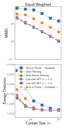
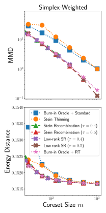
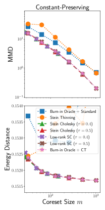
We next evaluate the practical utility of our procedures when faced with three common sources of bias: (1) burn-in, (2) approximate MCMC, and (3) tempering. In all experiments, we use a Stein kernel ${{\bm{k}}_{p}}$ with an inverse multiquadric (IMQ) base kernel ${\bm{k}}(x,y)\!=\!(1\!+\!\|{x\!-\!y}\|^{2}_{M}/\sigma^{2})^{-1/2}$ for $\sigma$ equal to the median pairwise $\|{\cdot}\|_{M}$ distance amongst $1000$ points standard thinned from the input. To vary output MMD precision, we first standard thin the input to size $n_{0}\in\{2^{10},2^{12},2^{14},2^{16},2^{18},2^{20}\}$ before applying any method, as discussed in Rems. 3 and 2. For low-rank or weighted coreset methods, we show results for $m\!=\!r\!=\!n^{\tau}$. When comparing weighted coresets, we optimally reweight every coreset. We report the median over 5 independent runs for all error metrics. We implement our algorithms in JAX (Bradbury et al., 2018) and refer the reader to App. I for additional experiment details.

Correcting for burn-in   The initial iterates of a Markov chain are biased by its starting point and need not accurately reflect the target distribution $\mathbb{P}$. Classical burn-in corrections use convergence diagnostics to detect and discard these iterates but typically require running multiple independent Markov chains (Cowles and Carlin, 1996). Alternatively, our proposed debiased compression methods can be used to correct for burn-in given just a single chain.

We test this claim using an experimental setup from Riabiz et al. (2022, Sec. 4.1) and the $6$-chain “burn-in oracle” diagnostic of Vats and Knudson (2021). We aim to compress a posterior $\mathbb{P}$ over the parameters in the Goodwin model of oscillatory enzymatic control ($d\!=\!4$) using $n\!=\!2\!\times\!10^{6}$ points from a preconditioned Metropolis-adjusted Langevin algorithm (P-MALA) chain. We repeat this experiment with three alternative MCMC algorithms in Sec. I.3. Our primary metric is $\operatorname{MMD}_{{{\bm{k}}_{\mathbb{P}}}}$ to $\mathbb{P}$ with $M=I$, but, for external validation, we also measure the energy distance (Riabiz et al., 2022, Eq. 11) to an auxiliary MCMC chain of length $n$. Trajectory plots of the first two coordinates (Fig. 1, left) highlight the substantial burn-in period for the Goodwin chain and the ability of LSKT to mimic the 6-chain burn-in oracle using only a single chain. In Fig. 1 (right), for both the MMD metric and the auxiliary energy distance, our proposed methods consistently outperform Stein thinning and match the quality of 6-chain burn-in removal paired with unbiased compression. The spike in baseline energy distance for the constant-preserving task can be attributed to the selection of overly large weight values due to poor matrix conditioning; the simplex-weighted task does not suffer from this issue due to its regularizing nonnegativity constraint.

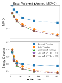
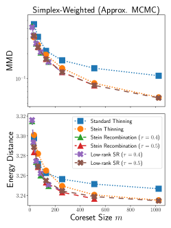
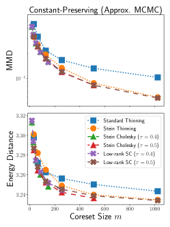
Correcting for approximate MCMC   In posterior inference, MCMC algorithms typically require iterating over every datapoint to draw each new sample point. When datasets are large, approximating MCMC using datapoint mini-batches can reduce sampling time at the cost of persistent bias and an unknown stationary distribution that prohibits debiasing via importance sampling. Our proposed methods can correct for these biases during compression by computing full-dataset scores on a small subset of $n_{0}$ standard thinned points. To evaluate this protocol, we compress a Bayesian logistic regression posterior conditioned on the Forest Covtype dataset ($d\!=\!54$) using $n\!=\!2^{24}$ approximate MCMC points from the stochastic gradient Fisher scoring sampler (Ahn et al., 2012) with batch size $32$. Following Wang et al. (2024), we set $M\!=\!-\nabla^{2}\!\log p(x_{\textup{mode}})$ at the sample mode $x_{\textup{mode}}$ and use $2^{20}$ surrogate ground truth points from the No U-turn Sampler (Hoffman et al., 2014) to evaluate energy distance. We find that our proposals improve upon standard thinning and Stein thinning for each compression task, not just in the optimized MMD metric (Fig. 2, top) but also in the auxiliary energy distance (Fig. 2, middle) and when measuring integration error for the mean (Fig. I.4).

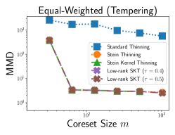
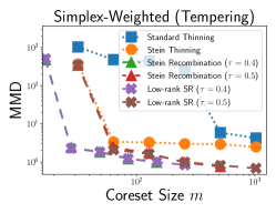
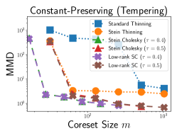
Correcting for tempering   Tempering, targeting a less-peaked and more dispersed distribution $\mathbb{Q}$, is a popular technique to improve the speed of MCMC convergence. One can correct for the sample bias using importance sampling, but this requires knowledge of the tempered density and can introduce substantial variance (Gramacy et al., 2010). Alternatively, one can use constructions of this work to correct for tempering during compression; this requires no importance weighting and no knowledge of $\mathbb{Q}$. To test this proposal, we compress the cardiac calcium signaling model posterior ($d=38$) of Riabiz et al. (2022, Sec. 4.3) with $M=I$ and $n=3\times 10^{6}$ tempered points from a Gaussian random walk Metropolis-Hastings chain. As discussed by Riabiz et al., compression is essential in this setting as the ultimate aim is to propagate posterior uncertainty through a human heart simulator, a feat which requires over $1000$ CPU hours for each summary point retained. Our methods perform on par with Stein thinning for equal-weighted compression and yield substantial gains over Stein (and standard) thinning for the two weighted compression tasks.

6 Conclusions and Future Work

We have introduced and analyzed a suite of new procedures for compressing a biased input sequence into an accurate summary of a target distribution. For equal-weighted compression, Stein kernel thinning delivers $\sqrt{n}$ points with $\widetilde{O}(n^{-1/2})$ MMD in $O(n^{2})$ time, and low-rank SKT can improve this running time to $\widetilde{O}(n^{3/2})$. For simplex-weighted and constant-preserving compression, Stein recombination and Stein Cholesky provide enhanced parsimony, matching these guarantees with as few as $\operatorname{poly-log}(n)$ points. Recent work has identified some limitations of score-based discrepancies, like Stein kernel MMDs, and developed modified objectives that are more sensitive to the relative density of isolated modes (Liu et al., 2023; Bénard et al., 2024). A valuable next step would be to extend our constructions to provide compression guarantees for these modified discrepancy measures. Other opportunities for future work include marrying the better-than-i.i.d. guarantees of this work with the non-myopic compression of Teymur et al. (2021), the control-variate compression of Chopin and Ducrocq (2021), and the online compression of Hawkins et al. (2022).

Broader Impact Statement

This paper presents work with the aim of advancing the field of Machine Learning. There are many potential societal consequences of our work, none which we feel must be specifically highlighted here.

Acknowledgments

We thank Marina Riabiz for making the Markov chain data used in Sec. 5 available and Jeffrey Rosenthal for helpful discussions concerning the geometric ergodicity of Markov chains.

References

  • Afzali and Muthukumarana (2023) E. Afzali and S. Muthukumarana. Gradient-free kernel conditional stein discrepancy goodness of fit testing. Machine Learning with Applications, 12:100463, 2023. ISSN 2666-8270. doi: https://doi.org/10.1016/j.mlwa.2023.100463. URL https://www.sciencedirect.com/science/article/pii/S2666827023000166.
  • Ahn et al. (2012) S. Ahn, A. Korattikara, and M. Welling. Bayesian posterior sampling via stochastic gradient fisher scoring. arXiv preprint arXiv:1206.6380, 2012.
  • Aronszajn (1950) N. Aronszajn. Theory of reproducing kernels. Transactions of the American mathematical society, 68(3):337–404, 1950.
  • Atchadé and Perron (2007) Y. F. Atchadé and F. Perron. On the geometric ergodicity of metropolis-hastings algorithms. Statistics, 41(1):77–84, 2007.
  • Barp et al. (2019) A. Barp, F.-X. Briol, A. Duncan, M. Girolami, and L. Mackey. Minimum stein discrepancy estimators. Advances in Neural Information Processing Systems, 32, 2019.
  • Barp et al. (2022) A. Barp, C.-J. Simon-Gabriel, M. Girolami, and L. Mackey. Targeted separation and convergence with kernel discrepancies. arXiv preprint arXiv:2209.12835, 2022.
  • Bénard et al. (2024) C. Bénard, B. Staber, and S. Da Veiga. Kernel stein discrepancy thinning: a theoretical perspective of pathologies and a practical fix with regularization. Advances in Neural Information Processing Systems, 36, 2024.
  • Billingsley (2013) P. Billingsley. Convergence of probability measures. John Wiley & Sons, 2013.
  • Bradbury et al. (2018) J. Bradbury, R. Frostig, P. Hawkins, M. J. Johnson, C. Leary, D. Maclaurin, G. Necula, A. Paszke, J. VanderPlas, S. Wanderman-Milne, and Q. Zhang. JAX: composable transformations of Python+NumPy programs, 2018. URL http://github.com/google/jax.
  • Bradley (2005) R. C. Bradley. Basic properties of strong mixing conditions. a survey and some open questions. 2005.
  • Carmeli et al. (2006) C. Carmeli, E. De Vito, and A. Toigo. Vector valued reproducing kernel hilbert spaces of integrable functions and mercer theorem. Analysis and Applications, 4(04):377–408, 2006.
  • Chandra (2015) T. K. Chandra. De la vallée poussin’s theorem, uniform integrability, tightness and moments. Statistics & Probability Letters, 107:136–141, 2015.
  • Chen et al. (2022) Y. Chen, E. N. Epperly, J. A. Tropp, and R. J. Webber. Randomly pivoted cholesky: Practical approximation of a kernel matrix with few entry evaluations. arXiv preprint arXiv:2207.06503, 2022.
  • Chopin and Ducrocq (2021) N. Chopin and G. Ducrocq. Fast compression of mcmc output. Entropy, 23(8):1017, 2021.
  • Chwialkowski et al. (2016) K. Chwialkowski, H. Strathmann, and A. Gretton. A kernel test of goodness of fit. In M. F. Balcan and K. Q. Weinberger, editors, Proceedings of The 33rd International Conference on Machine Learning, volume 48 of Proceedings of Machine Learning Research, pages 2606–2615, New York, New York, USA, 20–22 Jun 2016. PMLR. URL https://proceedings.mlr.press/v48/chwialkowski16.html.
  • Cowles and Carlin (1996) M. K. Cowles and B. P. Carlin. Markov chain monte carlo convergence diagnostics: a comparative review. Journal of the American Statistical Association, 91(434):883–904, 1996.
  • Dax et al. (2014) A. Dax et al. Low-rank positive approximants of symmetric matrices. Advances in Linear Algebra & Matrix Theory, 4(03):172, 2014.
  • Douc and Cappé (2005) R. Douc and O. Cappé. Comparison of resampling schemes for particle filtering. In ISPA 2005. Proceedings of the 4th International Symposium on Image and Signal Processing and Analysis, 2005., pages 64–69. IEEE, 2005.
  • Douc et al. (2018) R. Douc, E. Moulines, P. Priouret, and P. Soulier. Markov chains, volume 1. Springer, 2018.
  • Durmus and Moulines (2017) A. Durmus and E. Moulines. Nonasymptotic convergence analysis for the unadjusted langevin algorithm. 2017.
  • Durmus and Moulines (2022) A. Durmus and É. Moulines. On the geometric convergence for mala under verifiable conditions. arXiv preprint arXiv:2201.01951, 2022.
  • Durmus et al. (2020) A. Durmus, É. Moulines, and E. Saksman. Irreducibility and geometric ergodicity of hamiltonian monte carlo. The Annals of Statistics, 48(6):3545–3564, 2020.
  • Dwivedi and Mackey (2021) R. Dwivedi and L. Mackey. Kernel thinning. arXiv preprint arXiv:2105.05842, 2021.
  • Dwivedi and Mackey (2022) R. Dwivedi and L. Mackey. Generalized kernel thinning. In International Conference on Learning Representations, 2022.
  • Epperly and Moreno (2024) E. Epperly and E. Moreno. Kernel quadrature with randomly pivoted cholesky. Advances in Neural Information Processing Systems, 36, 2024.
  • Erdogdu et al. (2018) M. A. Erdogdu, L. Mackey, and O. Shamir. Global non-convex optimization with discretized diffusions. Advances in Neural Information Processing Systems, 31, 2018.
  • Gallegos-Herrada et al. (2023) M. A. Gallegos-Herrada, D. Ledvinka, and J. S. Rosenthal. Equivalences of geometric ergodicity of markov chains, 2023.
  • Ghojogh et al. (2021) B. Ghojogh, A. Ghodsi, F. Karray, and M. Crowley. Kkt conditions, first-order and second-order optimization, and distributed optimization: tutorial and survey. arXiv preprint arXiv:2110.01858, 2021.
  • Gorham and Mackey (2017) J. Gorham and L. Mackey. Measuring sample quality with kernels. In International Conference on Machine Learning, pages 1292–1301. PMLR, 2017.
  • Gorham et al. (2019) J. Gorham, A. B. Duncan, S. J. Vollmer, and L. Mackey. Measuring sample quality with diffusions. The Annals of Applied Probability, 29(5):2884–2928, 2019.
  • Gramacy et al. (2010) R. Gramacy, R. Samworth, and R. King. Importance tempering. Statistics and Computing, 20:1–7, 2010.
  • Gretton et al. (2012) A. Gretton, K. M. Borgwardt, M. J. Rasch, B. Schölkopf, and A. Smola. A kernel two-sample test. The Journal of Machine Learning Research, 13(1):723–773, 2012.
  • Hawkins et al. (2022) C. Hawkins, A. Koppel, and Z. Zhang. Online, informative mcmc thinning with kernelized stein discrepancy. arXiv preprint arXiv:2201.07130, 2022.
  • Hayakawa et al. (2022) S. Hayakawa, H. Oberhauser, and T. Lyons. Positively weighted kernel quadrature via subsampling. Advances in Neural Information Processing Systems, 35:6886–6900, 2022.
  • Hayakawa et al. (2023) S. Hayakawa, H. Oberhauser, and T. Lyons. Sampling-based nyström approximation and kernel quadrature. In Proceedings of the 40th International Conference on Machine Learning, ICML’23. JMLR.org, 2023.
  • Hodgkinson et al. (2020) L. Hodgkinson, R. Salomone, and F. Roosta. The reproducing stein kernel approach for post-hoc corrected sampling. arXiv preprint arXiv:2001.09266, 2020.
  • Hoffman et al. (2014) M. D. Hoffman, A. Gelman, et al. The no-u-turn sampler: adaptively setting path lengths in hamiltonian monte carlo. J. Mach. Learn. Res., 15(1):1593–1623, 2014.
  • Johnson (2009) A. A. Johnson. Geometric ergodicity of Gibbs samplers. university of minnesota, 2009.
  • Li et al. (2023) L. Li, J.-G. Liu, and Y. Wang. Geometric ergodicity of sgld via reflection coupling. arXiv preprint arXiv:2301.06769, 2023.
  • Liu and Lee (2017) Q. Liu and J. Lee. Black-box importance sampling. In Artificial Intelligence and Statistics, pages 952–961. PMLR, 2017.
  • Liu et al. (2016) Q. Liu, J. Lee, and M. Jordan. A kernelized stein discrepancy for goodness-of-fit tests. In International conference on machine learning, pages 276–284. PMLR, 2016.
  • Liu et al. (2023) X. Liu, A. B. Duncan, and A. Gandy. Using perturbation to improve goodness-of-fit tests based on kernelized stein discrepancy. In A. Krause, E. Brunskill, K. Cho, B. Engelhardt, S. Sabato, and J. Scarlett, editors, Proceedings of the 40th International Conference on Machine Learning, volume 202 of Proceedings of Machine Learning Research, pages 21527–21547. PMLR, 23–29 Jul 2023.
  • Merlevède et al. (1997) F. Merlevède, M. Peligrad, and S. Utev. Sharp conditions for the clt of linear processes in a hilbert space. Journal of Theoretical Probability, 10(3):681–693, 1997.
  • Meyn and Tweedie (2012) S. P. Meyn and R. L. Tweedie. Markov chains and stochastic stability. Springer Science & Business Media, 2012.
  • Minh (2010) H. Q. Minh. Some properties of gaussian reproducing kernel hilbert spaces and their implications for function approximation and learning theory. Constructive Approximation, 32:307–338, 2010.
  • Niederer et al. (2011) S. Niederer, L. Mitchell, N. Smith, and G. Plank. Simulating human cardiac electrophysiology on clinical time-scales. Frontiers in physiology, 2:14, 2011.
  • Paulsen and Raghupathi (2016) V. I. Paulsen and M. Raghupathi. An introduction to the theory of reproducing kernel Hilbert spaces, volume 152. Cambridge university press, 2016.
  • Phan et al. (2019) D. Phan, N. Pradhan, and M. Jankowiak. Composable effects for flexible and accelerated probabilistic programming in numpyro. arXiv preprint arXiv:1912.11554, 2019.
  • Pinelis (2020) I. Pinelis. Exact lower and upper bounds on the incomplete gamma function. arXiv preprint arXiv:2005.06384, 2020.
  • Pitcan (2017) Y. Pitcan. A note on concentration inequalities for u-statistics. arXiv preprint arXiv:1712.06160, 2017.
  • Qin (2023) Q. Qin. Geometric ergodicity of trans-dimensional markov chain monte carlo algorithms. arXiv preprint arXiv:2308.00139, 2023.
  • Riabiz et al. (2020) M. Riabiz, W. Y. Chen, J. Cockayne, P. Swietach, S. A. Niederer, L. Mackey, and C. J. Oates. Replication Data for: Optimal Thinning of MCMC Output, 2020. URL https://doi.org/10.7910/DVN/MDKNWM. Accessed on Mar 23, 2021.
  • Riabiz et al. (2022) M. Riabiz, W. Y. Chen, J. Cockayne, P. Swietach, S. A. Niederer, L. Mackey, and C. J. Oates. Optimal thinning of mcmc output. Journal of the Royal Statistical Society Series B: Statistical Methodology, 84(4):1059–1081, 2022.
  • Roberts and Tweedie (1996) G. O. Roberts and R. L. Tweedie. Geometric convergence and central limit theorems for multidimensional hastings and metropolis algorithms. Biometrika, 83(1):95–110, 1996.
  • Shetty et al. (2022) A. Shetty, R. Dwivedi, and L. Mackey. Distribution compression in near-linear time. In International Conference on Learning Representations, 2022.
  • Steinwart and Christmann (2008) I. Steinwart and A. Christmann. Support vector machines. Springer Science & Business Media, 2008.
  • Steinwart and Scovel (2012) I. Steinwart and C. Scovel. Mercer’s theorem on general domains: On the interaction between measures, kernels, and rkhss. Constructive Approximation, 35:363–417, 2012.
  • Sun and Zhou (2008) H.-W. Sun and D.-X. Zhou. Reproducing kernel hilbert spaces associated with analytic translation-invariant mercer kernels. Journal of Fourier Analysis and Applications, 14(1):89–101, 2008.
  • Tchernychova (2016) M. Tchernychova. Caratheodory cubature measures. PhD thesis, University of Oxford, 2016.
  • Teymur et al. (2021) O. Teymur, J. Gorham, M. Riabiz, and C. Oates. Optimal quantisation of probability measures using maximum mean discrepancy. In International Conference on Artificial Intelligence and Statistics, pages 1027–1035. PMLR, 2021.
  • Vats and Knudson (2021) D. Vats and C. Knudson. Revisiting the gelman–rubin diagnostic. Statistical Science, 36(4):518–529, 2021.
  • Wainwright (2019) M. J. Wainwright. High-dimensional statistics: A non-asymptotic viewpoint, volume 48. Cambridge university press, 2019.
  • Wang et al. (2024) C. Wang, Y. Chen, H. Kanagawa, and C. J. Oates. Stein $\Pi$-importance sampling. Advances in Neural Information Processing Systems, 36, 2024.
  • Wang et al. (2023) J.-K. Wang, J. Abernethy, and K. Y. Levy. No-regret dynamics in the fenchel game: A unified framework for algorithmic convex optimization. Mathematical Programming, pages 1–66, 2023.
  • Wellner et al. (2013) J. Wellner et al. Weak convergence and empirical processes: with applications to statistics. Springer Science & Business Media, 2013.
  • Yang et al. (2018) J. Yang, Q. Liu, V. Rao, and J. Neville. Goodness-of-fit testing for discrete distributions via stein discrepancy. In International Conference on Machine Learning, pages 5561–5570. PMLR, 2018.
  • Zhang (2006) F. Zhang. The Schur complement and its applications, volume 4. Springer Science & Business Media, 2006.
  • Zhou (2002) D.-X. Zhou. The covering number in learning theory. Journal of Complexity, 18(3):739–767, 2002.
\etoctocstyle

1Appendix Contents \etocdepthtag.tocmtappendix \etocsettagdepthmtchapternone \etocsettagdepthmtappendixsection \etocsettagdepthmtappendixsubsection \etocsettagdepthmtappendixsubsubsection

Appendix A Appendix Notation

For the point sequence $\mathcal{S}_{n}=(x_{i})_{i\in[n]}$, we define $\mathbb{S}_{n}\triangleq\frac{1}{n}\sum_{i\in[n]}\delta_{x_{i}}$. For a weight vector $w\in\mathbb{R}^{n}$, we define the support $\operatorname{supp}(w)\triangleq\{i\in[n]:w_{i}\neq 0\}$ and the signed measure $\mathbb{S}_{n}^{w}\triangleq\sum_{i\in[n]}w_{i}\delta_{x_{i}}$. For a matrix $K\in\mathbb{R}^{n\times n}$ and $w\in\Delta_{n-1}$, we define the weighted matrix $K^{w}\triangleq\operatorname{diag}(\sqrt{w})K\operatorname{diag}(\sqrt{w})$. For positive semidefinite (PSD) matrices $(A,B)$, we use $A\succeq B$ (resp. $A\preceq B$) to mean $A-B$ (resp. $B-A$) is PSD. For a symmetric PSD (SPSD) matrix $M$, we let $M^{1/2}$ denote a symmetric matrix square root satisfying $M=M^{1/2}M^{1/2}$. For $A\in\mathbb{R}^{n\times m}$, we denote $\left\|{A}\right\|_{p}\triangleq\sup_{x\neq 0}\frac{\left\|{Ax}\right\|_{p}}{\left\|{x}\right\|_{p}}$. We will use $\mathbbm{1}_{E}$ to denote the indicator function for an event $E$.

Notations used only in a specific section will be introduced within.

Appendix B Spectral Analysis of Kernel Matrices

The goal of this section is to develop spectral bounds for kernel matrices.

In Sec. B.1, we transfer the bounds on covering numbers from the definition of PolyGrowth or LogGrowth kernels to bounds on the eigenvalues of the kernel matrices. This sets the theoretical foundation for the algorithms in later sections as their error guarantees rely on the fast decay of eigenvalues of kernel matrices.

In Sec. B.2, we show that Stein kernels are PolyGrowth (resp. LogGrowth) provided that their base kernels are differentiable (resp. radially analytic). Hence we obtain spectral bounds for a wide range of Stein kernels.

Notation   For a normed space $E$, we use $\left\|{\cdot}\right\|_{E}$ to denote its norm, $\mathcal{B}_{E}(p,r)\triangleq\{x\in E:\left\|{x-p}\right\|_{E}\leq r\}$ to denote the closed ball of radius $r$ centered at $p$ in $E$ with the shorthand $\mathcal{B}_{E}(r)\triangleq\mathcal{B}_{E}(0,r)$ and $\mathcal{B}_{E}\triangleq\mathcal{B}_{E}(1)$. When $E$ is an RKHS with kernel ${\bm{k}}$, for brevity we use ${\bm{k}}$ in place of $E$ in the subscript. Let $\mathfrak{F}(\mathcal{X},\mathcal{Y})$ denote the space of functions from $\mathcal{X}$ to $\mathcal{Y}$, and $\mathfrak{B}(E,F)$ denote the space of bounded linear functions between normed spaces $E,F$. For a set $A$, we use $\ell_{\infty}(A)$ to denote the space of bounded $\mathbb{R}$-valued functions on $A$ equipped with the sup-norm $\left\|{f}\right\|_{\infty,A}\triangleq\sup_{x\in A}|f(x)|$. We use ${E}\hookrightarrow{F}$ to denote the inclusion map. e use $\lambda_{\ell}(T)$ to denote the $\ell$-th largest eigenvalue of an operator $T$.

B.1 Bounding the spectrum of kernel matrices

We first introduce the general Mercer representation theorem from Steinwart and Scovel [2012], which shows the existence of a discrete spectrum of the integral operator associated with a continuous square-integrable kernel. The theorem also provides a series expansion of the kernel, i.e., the Mercer representation, in terms of the eigenvalues and eigenfunctions.

Lemma B.1 (General Mercer representation [Steinwart and Scovel, 2012]).

Consider a kernel ${\bm{k}}:\mathbb{R}^{d}\times\mathbb{R}^{d}\to\mathbb{R}$ that is jointly continuous in both inputs and a probability measure $\mu$ such that $\int{\bm{k}}(x,x)\differential\mu(x)<\infty$. Then the following holds.

  1. (a)

    The inclusion ${{\mathcal{H}_{{\bm{k}}}}}\hookrightarrow{\mathcal{L}^{2}(\mu)}$ is a compact operator, i.e., $\mathcal{B}_{{\bm{k}}}$ is a compact subset of $\mathcal{L}^{2}(\mu)$. In particular, this inclusion is continuous.

  2. (b)

    The Hilbert-space adjoint of the inclusion ${{\mathcal{H}_{{\bm{k}}}}}\hookrightarrow{\mathcal{L}^{2}(\mu)}$ is the compact operator $S_{{\bm{k}},\mu}:\mathcal{L}^{2}(\mu)\to{\mathcal{H}_{{\bm{k}}}}$ defined as

    $\textstyle S_{{\bm{k}},\mu}f\triangleq\int{\bm{k}}(\cdot,x)f(x)\differential\mu(x).$ (22)

    We also have $S_{{\bm{k}},\mu}^{*}\triangleq{{\mathcal{H}_{{\bm{k}}}}}\hookrightarrow{\mathcal{L}^{2}(\mu)}$. Hence the operator

    $\textstyle T_{{\bm{k}},\mu}\triangleq S^{*}_{{\bm{k}},\mu}S_{{\bm{k}},\mu}:\mathcal{L}^{2}(\mu)\to\mathcal{L}^{2}(\mu)$ (23)

    is also compact.

  3. (c)

    There exist $\{\lambda_{\ell}\}_{\ell=1}^{\infty}$ with $\lambda_{1}\geq\lambda_{2}\geq\cdots\geq 0$ and $\{\phi_{\ell}\}_{\ell=1}^{\infty}\subset{\mathcal{H}_{{\bm{k}}}}$ such that $\{{\phi_{\ell}}\}_{\ell=1}^{\infty}$ is an orthonormal system in $\mathcal{L}^{2}(\mu)$ and $\{\lambda_{\ell}\}_{\ell=1}^{\infty}$ (resp. $\{{\phi_{\ell}}\}_{\ell=1}^{\infty}$) consists of the eigenvalues (resp. eigenfunctions) of $T_{{\bm{k}},\mu}$ with eigendecomposition, for ${f}\in\mathcal{L}^{2}(\mu)$,

    $\textstyle T_{{\bm{k}},\mu}{f}=\sum_{\ell=1}^{\infty}\lambda_{\ell}\langle{f},{\phi_{\ell}}\rangle_{\mathcal{L}^{2}(\mu)}{\phi_{\ell}}$ (24)

    with convergence in $\mathcal{L}^{2}(\mu)$.

  4. (d)

    We have the following series expansion

    $\textstyle{\bm{k}}(x,x^{\prime})$ $\textstyle=\sum_{\ell=1}^{\infty}\lambda_{i}\phi_{\ell}(x)\phi_{\ell}(x^{\prime}),$ (25)

    where the series convergence is absolute and uniform in $x,x^{\prime}$ on all $A\times A\subset\operatorname{supp}\mu\times\operatorname{supp}\mu$.

Proof of Lem. B.1.

Part (a) and (b) follow respectively from Steinwart and Scovel [2012, Lem. 2.3 and 2.2]. Part (c) follows from part (a) and Steinwart and Scovel [2012, Lem. 2.12]. Finally, part (d) follows from Steinwart and Scovel [2012, Cor. 3.5]. ∎

We will use the following lemma regarding the restriction of covering numbers.

Lemma B.2 (Covering number is preserved in restriction).

For a kernel ${\bm{k}}:\mathbb{R}^{d}\times\mathbb{R}^{d}\to\mathbb{R}$ and a set $A\subset\mathbb{R}^{d}$, we have $\mathcal{N}_{{\bm{k}}}(A,\epsilon)=\mathcal{N}_{{\bm{k}}|_{A}}(A,\epsilon)$, for ${\bm{k}}|_{A}$, the restricted kernel of ${\bm{k}}$ to $A$ [Paulsen and Raghupathi, 2016, Sec. 5.4].

Proof of Lem. B.2.

It suffices to show that a $({\bm{k}},A,\epsilon)$ cover can be converted to a cover of $({\bm{k}}|_{A},A,\epsilon)$ of the same cardinality and vice versa.

Let $\mathcal{C}\subset\mathcal{B}_{{\bm{k}}|_{A}}$ be a $({\bm{k}}|_{A},A,\epsilon)$ cover. For any $f\in\mathcal{C}$, we have $\|{f}\|_{{\bm{k}}|_{A}}=\inf\left\{\|{\tilde{f}}\|_{{\bm{k}}}:\tilde{f}\in{\mathcal{H}_{{\bm{k}}}},\tilde{f}|_{A}=f\right\}\leq 1$ [Paulsen and Raghupathi, 2016, Corollary 5.8]. Moreover, the infimum is attained by some $\tilde{f}\in{\mathcal{H}_{{\bm{k}}}}$ such that $\|{\tilde{f}}\|_{{\bm{k}}}=\|{f}\|_{{\bm{k}}|_{A}}\leq 1$ and $\tilde{f}|_{A}=f$. Now form $\tilde{\mathcal{C}}=\{\tilde{f}:f\in\mathcal{C}\}$. For any $\tilde{h}\in\mathcal{B}_{{\bm{k}}}$, there exists $f\in\mathcal{C}$ such that

$\textstyle\left\|{\tilde{h}|_{A}-f}\right\|_{\infty,A}\leq\epsilon\implies=\left\|{\tilde{h}-\tilde{f}}\right\|_{\infty,A}\leq\epsilon,$ (26)

so $\tilde{\mathcal{C}}$ is a $({\bm{k}}|_{A},A,\epsilon)$ cover.

For the other direction, let $\tilde{\mathcal{C}}\subset\mathcal{B}_{{\bm{k}}}$ be a $({\bm{k}},A,\epsilon)$ cover. Define $\mathcal{C}=\{\tilde{f}|_{A}:\tilde{f}\in\tilde{\mathcal{C}}\}\subset{\mathcal{H}_{{\bm{k}}|_{A}}}$. Since $\|{\tilde{f}|_{A}}\|_{{\bm{k}}|_{A}}\leq\|{\tilde{f}}\|_{{\bm{k}}}$, we have $\mathcal{C}\subset\mathcal{B}_{{\bm{k}}|_{A}}$. For any $h\in\mathcal{B}_{{\bm{k}}_{A}]}$, again by Paulsen and Raghupathi [2016, Corollary 5.8], there exists $\tilde{h}\in{\mathcal{H}_{{\bm{k}}}}$ such that $\|{\tilde{h}}\|_{{\bm{k}}}=\|{h}\|_{{\bm{k}}|_{A}}\leq 1$, so there exists $\tilde{f}\in\tilde{\mathcal{C}}$ such that

$\textstyle\left\|{\tilde{h}-\tilde{f}}\right\|_{\infty,A}\leq\epsilon\implies\left\|{h-\tilde{f}|_{A}}\right\|_{\infty,A}\leq\epsilon,$ (27)

Hence $\mathcal{C}$ is a $({\bm{k}},A,\epsilon)$ cover. ∎

The goal for the rest of this section is to transfer the bounds of the covering number in the definition of a PolyGrowth or LogGrowth kernel from Assum. ($\bm{{\alpha},{\beta}}$)-kernel to bounds on entropy numbers [Steinwart and Christmann, 2008, Def. 6.20] that are closely related to eigenvalues of the integral operator (23).

Definition B.1 (Entropy number of a bounded linear map).

For a bounded linear operator $S:E\to F$ between normed spaces $E,F$, for $\ell\in\mathbb{N}$, the $\ell$-th entropy number of $S$ is defined as

$\textstyle e_{\ell}(S)\triangleq\inf\left\{\epsilon>0:\exists s_{1},\ldots,s_{2^{\ell-1}}\in S(\mathcal{B}_{E})\text{ such that }S(\mathcal{B}_{E})\subset\bigcup_{i=1}^{2^{\ell-1}}\mathcal{B}_{F}(s_{i},\epsilon)\right\}.$ (28)

The following lemma shows the relation between covering numbers and entropy numbers.

Lemma B.3 (Relation between covering number and entropy number).

Suppose a kernel ${\bm{k}}$ is jointly continuous and $A\subset\mathbb{R}^{d}$ is bounded. Then for any $\epsilon>0$,

$\textstyle e_{\lceil\log_{2}\mathcal{N}_{{\bm{k}}}(A,\epsilon)\rceil+1}({{\mathcal{H}_{{\bm{k}}|_{A}}}}\hookrightarrow{\ell_{\infty}(A)})\leq\epsilon.$ (29)
Proof of Lem. B.3.

First, the assumption implies ${\bm{k}}|_{A}$ is a bounded kernel, so by Steinwart and Christmann [2008, Lemma 4.23], the inclusion ${{\mathcal{H}_{{\bm{k}}|_{A}}}}\hookrightarrow{\ell_{\infty}(A)}$ is continuous. By the definition of $\mathcal{N}_{{\bm{k}}|_{A}}(A,\epsilon)$, by adding arbitrary elements into the cover if necessary, there exists a $({\bm{k}}|_{A},A,\epsilon)$ cover of $\mathcal{B}_{{\bm{k}}|_{A}}$ of cardinality $2^{\lceil\log_{2}(\mathcal{N}_{{\bm{k}}|_{A}}(A,\epsilon))\rceil}\geq\mathcal{N}_{{\bm{k}}|_{A}}(A,\epsilon)$. Hence

$\textstyle e_{\lceil\log_{2}\mathcal{N}_{{\bm{k}}|_{A}}(A,\epsilon)\rceil+1}({{\mathcal{H}_{{\bm{k}}|_{A}}}}\hookrightarrow{\ell_{\infty}(A)})\leq\epsilon.$ (30)

The claim follows since $\mathcal{N}_{{\bm{k}}|_{A}}(A,\epsilon)=\mathcal{N}_{{\bm{k}}}(A,\epsilon)$ by Lem. B.2. ∎

Proposition B.1 ($\ell_{\infty}$-entropy number bound for PolyGrowth or LogGrowth ${\bm{k}}$).

Suppose a kernel ${\bm{k}}$ satisfies Assum. ($\bm{{\alpha},{\beta}}$)-kernel. Let $\mathfrak{C}_{d}>0$ denote the constant that appears in the Assum. ($\bm{{\alpha},{\beta}}$)-kernel. Define

$\textstyle L_{\bm{k}}(r)\triangleq\frac{\mathfrak{C}_{d}}{\log 2}r^{\beta}.$ (31)

Then for any $r>0$ and $\ell\in\mathbb{N}$ that satisfies $\ell>L_{\bm{k}}(r+1)+1$, we have

e(𝒌|2(r)(2(r))){(L𝒌(r+1)1)1αif 𝒌isPolyGrowth(α,β), andexp(1(1L𝒌(r+1))1α)if 𝒌isLogGrowth(α,β).subscript𝑒subscriptevaluated-at𝒌subscript2𝑟subscriptsubscript2𝑟casessuperscriptsubscript𝐿𝒌𝑟111𝛼if 𝒌isPolyGrowth𝛼𝛽 and1superscript1subscript𝐿𝒌𝑟11𝛼if 𝒌isLogGrowth𝛼𝛽\textstyle e_{\ell}({{\mathcal{H}_{{\bm{k}}|_{\mathcal{B}_{2}(r)}}}}\hookrightarrow{\ell_{\infty}(\mathcal{B}_{2}(r))})\leq\begin{cases}\left(\frac{L_{\bm{k}}(r+1)}{\ell-1}\right)^{\frac{1}{{\alpha}}}&\text{if }{\bm{k}}\ \text{is}\ \hyperref@@ii[assum:kernel_growth]{\color[rgb]{0,0,0}{\textsc{PolyGrowth}}}(\alpha,\beta),\text{ and}\\ \exp(1-\left(\frac{\ell-1}{L_{\bm{k}}(r+1)}\right)^{\frac{1}{{\alpha}}})&\text{if }{\bm{k}}\ \text{is}\ \hyperref@@ii[assum:kernel_growth]{\color[rgb]{0,0,0}{\textsc{LogGrowth}}}(\alpha,\beta).\end{cases} (32)
Proof of Prop. B.1.

By Lem. B.3 and the fact that $e_{\ell}$ is monotonically decreasing in $\ell$ by definition, if $\ell\geq\log_{2}\mathcal{N}_{{\bm{k}}}(\mathcal{B}_{2}(r),\epsilon)+1$ for some $\epsilon>0$, then

$\textstyle e_{\ell}({{\mathcal{H}_{{\bm{k}}|_{\mathcal{B}_{2}(r)}}}}\hookrightarrow{\ell_{\infty}(\mathcal{B}_{2}(r))})\leq e_{\lceil\log_{2}\mathcal{N}_{{\bm{k}}}(\mathcal{B}_{2}(r),\epsilon)\rceil+1}({{\mathcal{H}_{{\bm{k}}|_{\mathcal{B}_{2}(r)}}}}\hookrightarrow{\ell_{\infty}(\mathcal{B}_{2}(r))})\leq\epsilon.$ (33)

For the PolyGrowth case, by its definition, the condition $\ell\geq\log_{2}\mathcal{N}_{{\bm{k}}}(\mathcal{B}_{2}(r),\epsilon)+1$ is met if $\epsilon\in(0,1)$ and

$\textstyle\ell\geq\frac{\mathfrak{C}_{d}}{\log 2}(1/\epsilon)^{{\alpha}}(r+1)^{\beta}+1\Longleftrightarrow\epsilon\leq\left(\frac{L_{\bm{k}}(r+1)}{\ell-1}\right)^{\frac{1}{{\alpha}}}.$ (34)

Hence (33) holds with $\epsilon=\left(\frac{L_{\bm{k}}(r+1)}{\ell-1}\right)^{\frac{1}{{\alpha}}}$, as long as $\epsilon\in(0,1)$, so $\ell$ needs to satisfy

$\textstyle 1$ $\textstyle>\left(\frac{L_{\bm{k}}(r+1)}{\ell-1}\right)^{\frac{1}{{\alpha}}}\Longleftrightarrow\ell>L_{\bm{k}}(r+1)+1.$ (35)

Similarly, for the LogGrowth case, the condition $\ell\geq\log_{2}\mathcal{N}_{{\bm{k}}}(\mathcal{B}_{2}(r),\epsilon)+1$ is met if $\epsilon\in(0,1)$ and

$\textstyle\ell\geq\frac{\mathfrak{C}_{d}}{\log 2}(\log(1/\epsilon)+1)^{{\alpha}}(r+1)^{\beta}+1\Longleftrightarrow\epsilon\leq\exp(1-\left(\frac{\ell-1}{L_{\bm{k}}(r+1)}\right)^{\frac{1}{{\alpha}}}).$ (36)

Hence (33) holds with $\epsilon=\exp(1-\left(\frac{\ell-1}{L_{\bm{k}}(r+1)}\right)^{\frac{1}{{\alpha}}})$, as long as $\epsilon\in(0,1)$, so $\ell$ needs to satisfy

$\textstyle 1$ $\textstyle>\exp(1-\left(\frac{\ell-1}{L_{\bm{k}}(r+1)}\right)^{\frac{1}{{\alpha}}})\Longleftrightarrow\ell>L_{\bm{k}}(r+1)+1.$ (37)

Next, we show that we can transfer bounds on entropy numbers to obtain bounds for the eigenvalues of kernel matrices, which will become handy when we develop sub-quadratic-time algorithms in Sec. 3. We rely on the following lemma, which summarizes the relevant facts from Steinwart and Christmann [2008, Appendix A].

Lemma B.4 (Eigenvalue is bounded by entropy number).

Let ${\bm{k}}$ be a jointly continuous kernel and $\mathbb{P}$ be a distribution such that $\mathbb{E}_{x\sim\mathbb{P}}[{\bm{k}}(x,x)]<\infty$, and recall that $\lambda_{\ell}(\cdot)$ denotes the $\ell$-th largest eigenvalue of a linear operator. Then, for all $\ell\in\mathbb{N}$,

$\textstyle\lambda_{\ell}(T_{{\bm{k}},\mathbb{P}})\leq 4e_{\ell}^{2}({{\mathcal{H}_{{\bm{k}}}}}\hookrightarrow{\mathcal{L}^{2}(\mathbb{P})}).$ (38)
Proof of Lem. B.4.

For any bounded linear operator $S:\mathcal{H}_{1}\to\mathcal{H}_{2}$ between Hilbert spaces $\mathcal{H}_{1}$ and $\mathcal{H}_{2}$, we have $a_{\ell}(S)\leq 2e_{\ell}(S)$, where $a_{\ell}$ is the $\ell$-th approximation number defined in Steinwart and Christmann [2008, (A.29)]. Recall the operator $S^{*}_{{\bm{k}},\mathbb{P}}={{\mathcal{H}_{{\bm{k}}}}}\hookrightarrow{\mathcal{L}^{2}(\mathbb{P})}$ from (22), which is compact (in particular bounded) by Lem. B.1(a). Thus

$\textstyle s_{\ell}(S^{*}_{{\bm{k}},\mathbb{P}})=a_{\ell}(S^{*}_{{\bm{k}},\mathbb{P}})\leq 2e_{\ell}(S^{*}_{{\bm{k}},\mathbb{P}}),$ (39)

where the first equality follows from the paragraph below Steinwart and Christmann [2008, (A.29)]) and $s_{\ell}$ is $\ell$-th singular number of an operator [Steinwart and Christmann, 2008, (A.25)]. Then using the identities mentioned under Steinwart and Christmann [2008, (A.25)] and Steinwart and Christmann [2008, (A.27)] and that all operators involved are compact by Lem. B.1(b), we have

$\textstyle\lambda_{\ell}(T_{{\bm{k}},\mathbb{P}})=\lambda_{\ell}(S^{*}_{{\bm{k}},\mathbb{P}}S_{{\bm{k}},\mathbb{P}})=s_{\ell}(S^{*}_{{\bm{k}},\mathbb{P}}S_{{\bm{k}},\mathbb{P}})=s^{2}_{\ell}(S^{*}_{{\bm{k}},\mathbb{P}})\leq 4e^{2}_{\ell}(S^{*}_{{\bm{k}},\mathbb{P}}).$ (40)

The previous lemma allows us to bound eigenvalues of kernel matrices by $\ell_{\infty}$-entropy numbers.

Proposition B.2 (Eigenvalue of kernel matrix is bounded by $\ell_{\infty}$-entropy number).

Let ${\bm{k}}$ be a jointly continuous kernel. Define $K\triangleq{\bm{k}}(\mathcal{S}_{n},\mathcal{S}_{n})$ for the sequence of points $\mathcal{S}_{n}=(x_{1},\ldots,x_{n})\subset\mathbb{R}^{d}$. For any $w\in\Delta_{n-1}$, recall the notation $\mathbb{S}_{n}^{w}=\sum_{i\in[n]}w_{i}\delta_{x_{i}}$, $K^{w}=\operatorname{diag}(\sqrt{w})K\operatorname{diag}(\sqrt{w})$, and $R_{n}=1+\sup_{i\in[n]}\left\|{x_{i}}\right\|_{2}$. Then for all $\ell\in\mathbb{N}$,

$\textstyle\lambda_{\ell}(K^{w})\stackrel{{\scriptstyle(i)}}{{=}}\lambda_{\ell}(T_{{\bm{k}},\mathbb{S}_{n}^{w}})\stackrel{{\scriptstyle(ii)}}{{\leq}}4e^{2}_{\ell}({{\mathcal{H}_{{\bm{k}}}}_{|_{\mathcal{B}_{2}(R_{n}-1)}}}\hookrightarrow{\ell_{\infty}(\mathcal{B}_{2}(R_{n}-1))}).$ (41)
Proof of Prop. B.2.

Without loss of generality, we assume $w_{i}>0$ for all $i\in[n]$, since otherwise, we can consider a smaller set of points by removing the ones with zero weights.

Proof of equality (i) from display 41   Note that $\mathcal{L}^{2}(\mathbb{S}_{n}^{w})$ is isometric to $\mathbb{R}^{n}$. Let $K\triangleq{\bm{k}}(\mathcal{S}_{n},\mathcal{S}_{n})$ denote the kernel matrix. The action of $T_{{\bm{k}},\mathbb{S}_{n}^{w}}$ is given by, for $i\in[n]$,

$\textstyle T_{{\bm{k}},\mathbb{S}_{n}^{w}}f(x_{i})=\sum_{j\in[n]}w_{j}{\bm{k}}(x_{i},x_{j})f(x_{j}),$ (42)

so in matrix form, $T_{{\bm{k}},\mathbb{S}_{n}^{w}}f=K\operatorname{diag}(w)f$, and hence $T_{{\bm{k}},\mathbb{S}^{w}_{n}}=K\operatorname{diag}(w)$. If $\lambda_{\ell}$ is an eigenvalue of $K\operatorname{diag}(w)$ with eigenvector $v_{\ell}$, then

$\textstyle K\operatorname{diag}(w)v_{\ell}=\lambda_{\ell}v_{\ell}$ $\textstyle\Longleftrightarrow\operatorname{diag}(\sqrt{w})K\operatorname{diag}(w)v_{\ell}=\lambda_{\ell}\operatorname{diag}(\sqrt{w})v_{\ell}$ (43)
$\textstyle\Longleftrightarrow\operatorname{diag}(\sqrt{w})K\operatorname{diag}(\sqrt{w})(\operatorname{diag}(\sqrt{w})v_{\ell})=\lambda_{\ell}\operatorname{diag}(\sqrt{w})v_{\ell},$ (44)

where we used $w_{i}>0$ for all $i\in[n]$. Hence the eigenspectrum of $T_{{\bm{k}},\mathbb{S}_{n}^{w}}$ agrees with that of $\operatorname{diag}(\sqrt{w})K\operatorname{diag}(\sqrt{w})$.

Proof of bound (ii) from display 41   By Lem. B.4, we have $\lambda_{\ell}(T_{{\bm{k}},\mathbb{S}_{n}^{w}})\leq 4e^{2}_{\ell}({{\mathcal{H}_{{\bm{k}}|_{\mathcal{B}_{2}(R_{n}-1)}}}}\hookrightarrow{\mathcal{L}^{2}(\mathbb{S}_{n}^{w})})$. Finally, using Def. B.1, we have $e_{\ell}({{\mathcal{H}_{{\bm{k}}|_{\mathcal{B}_{2}(R_{n}-1)}}}}\hookrightarrow{\mathcal{L}^{2}(\mathbb{S}_{n}^{w})})\leq e_{\ell}({{\mathcal{H}_{{\bm{k}}|_{\mathcal{B}_{2}(R_{n}-1)}}}}\hookrightarrow{\ell_{\infty}(\mathcal{B}_{2}(R_{n}-1))})$ because $\mathbb{S}_{n}^{w}$ is supported in $\mathcal{B}_{2}(R_{n}-1)$ and the fact that $\|{\cdot}\|_{\mathcal{L}^{2}(\mathbb{P})}\leq\|{\cdot}\|_{\infty}$ for any $\mathbb{P}$. ∎

Combining the tools developed so far, we have the following corollary for bounding the eigenvalues of PolyGrowth and LogGrowth kernel matrices.

Corollary B.1 (Eigenvalue bound for PolyGrowth or LogGrowth kernel matrix).

Suppose a kernel ${\bm{k}}$ satisfies Assum. ($\bm{{\alpha},{\beta}}$)-kernel. Let $\mathcal{S}_{n}=(x_{1},\ldots,x_{n})\subset\mathbb{R}^{d}$ be a sequence of points. For any $w\in\Delta_{n-1}$, using the notation $L_{\bm{k}}$ from (31), for any $\ell>L_{\bm{k}}(R_{n})+1$, we have

λ(Kw){4(L𝒌(Rn)1)2αPolyGrowth(α,β)and4exp(22(1L𝒌(Rn))1α)LogGrowth(α,β).subscript𝜆superscript𝐾𝑤cases4superscriptsubscript𝐿𝒌subscript𝑅𝑛12𝛼PolyGrowth𝛼𝛽and422superscript1subscript𝐿𝒌subscript𝑅𝑛1𝛼LogGrowth𝛼𝛽\textstyle\lambda_{\ell}(K^{w})\leq\begin{cases}4\left(\frac{L_{\bm{k}}(R_{n})}{\ell-1}\right)^{\frac{2}{{\alpha}}}&\hyperref@@ii[assum:kernel_growth]{\color[rgb]{0,0,0}{\textsc{PolyGrowth}}}(\alpha,\beta)\quad\text{and}\\ 4\exp(2-2\left(\frac{\ell-1}{L_{\bm{k}}(R_{n})}\right)^{\frac{1}{{\alpha}}})&\hyperref@@ii[assum:kernel_growth]{\color[rgb]{0,0,0}{\textsc{LogGrowth}}}(\alpha,\beta).\end{cases} (45)
Proof of Cor. B.1.

The claim follows by applying Prop. B.2 and Prop. B.1. ∎

B.2 Spectral decay of Stein kernels

The goal of this section is to show that a Stein kernel ${{\bm{k}}_{p}}$ satisfies Assum. ($\bm{{\alpha},{\beta}}$)-kernel provided that the base kernel is sufficiently smooth and to derive the parameters ${\alpha}$, ${\beta}$ for PolyGrowth and LogGrowth cases.

For a Stein kernel ${{\bm{k}}_{p}}$ with preconditioning matrix $M$, we define

$\textstyle\mathfrak{S}_{p}(r)\triangleq\max\left(1,\sup_{\left\|{x}\right\|_{2}\leq r}\left\|{M^{1/2}\nabla\log p(x)}\right\|_{2}\right).$ (46)

We start by noting a useful alternative expression for a Stein kernel where we only need access to the density via the score $\nabla\log p$.

Proposition B.3 (Alternative expression for Stein kernel).

The Stein kernel ${{\bm{k}}_{p}}$ has the following alternative form:

$\textstyle\begin{split}\textstyle{{\bm{k}}_{p}}(x,y)=\langle\nabla\log p(x),M\nabla\log p(y)\rangle{\bm{k}}(x,y)+\langle\nabla\log p(x),M\nabla_{y}{\bm{k}}(x,y)\rangle+\\ \textstyle\langle\nabla\log p(y),M\nabla_{x}{\bm{k}}(x,y)\rangle+\tr(M\nabla_{x}\nabla_{y}{\bm{k}}(x,y)),\end{split}$ (47)

where $\nabla_{x}\nabla_{y}{\bm{k}}(x,y)$ denotes the $d\times d$ matrix $(\partial_{x_{i}}\partial_{y_{j}}{\bm{k}}(x,y))_{i,j\in[d]}$.

Proof of Prop. B.3.

We compute

$\textstyle(\nabla_{x}\cdot(p(x)M{\bm{k}}(x,y)p(y)))_{j}$ $\textstyle=\sum_{i\in[d]}M_{ij}\left(\partial_{x_{i}}p(x){\bm{k}}(x,y)p(y)+p(x)\partial_{x_{i}}{\bm{k}}(x,y)p(y)\right).$ (48)
$\textstyle\begin{split}\textstyle\nabla_{y}\cdot\nabla_{x}\cdot(p(x)M{\bm{k}}(x,y)p(y))&\textstyle=\sum_{i,j\in[d]}M_{ij}\left(\partial_{x_{i}}p(x)\partial_{y_{j}}p(y){\bm{k}}(x,y)+\partial_{x_{i}}p(x)\partial_{y_{j}}{\bm{k}}(x,y)p(y)\right)\\ \textstyle&\textstyle+\sum_{i,j\in[d]}M_{ij}\left(p(x)\partial_{y_{j}}p(y)\partial_{x_{i}}{\bm{k}}(x,y)+p(x)\partial_{x_{i}}\partial_{y_{j}}{\bm{k}}(x,y)p(y)\right).\end{split}$ (49)

The four terms in the last equation correspond to the four terms in (47). ∎

In what follows, we will make use of a matrix-valued kernel ${\bm{K}}:\mathbb{R}^{d}\times\mathbb{R}^{d}\to\mathbb{R}^{d\times d}$ which generates an RKHS ${\mathcal{H}_{{\bm{K}}}}$ of vector-valued functions. See Carmeli et al. [2006] for an introduction to vector-valued RKHS theory.

Our next goal is to build a Hilbert-space isometry between the direct sum Hilbert space ${\mathcal{H}_{{\bm{k}}}}^{\oplus d}$ and ${\mathcal{H}_{{{\bm{k}}_{p}}}}$ to represent functions in ${\mathcal{H}_{{{\bm{k}}_{p}}}}$ using functions from ${\mathcal{H}_{{\bm{k}}}}$.

Lemma B.5 (Preconditioned matrix-valued RKHS from a scalar kernel).

Let ${\bm{k}}:\mathbb{R}^{d}\times\mathbb{R}^{d}\to\mathbb{R}$ be kernel and ${\mathcal{H}_{{\bm{k}}}}$ be the corresponding RKHS. Let $M\in\mathbb{R}^{d\times d}$ be an SPSD matrix. Consider the map $\iota:{\mathcal{H}_{{\bm{k}}}}^{\oplus d}\to\mathfrak{F}(\mathbb{R}^{d},\mathbb{R}^{d})$ defined by $(f_{1},\ldots,f_{d})\mapsto[x\mapsto M^{1/2}(f_{1}(x),\ldots,f_{d}(x))]$, where ${\mathcal{H}_{{\bm{k}}}}^{\oplus d}$ is the direct-sum Hilbert space of $d$ copies of ${\mathcal{H}_{{\bm{k}}}}$ Then $\iota$ is a Hilbert-space isometry onto a vector-valued RKHS ${\mathcal{H}_{{\bm{K}}}}$ with matrix-valued reproducing kernel given by ${\bm{K}}(x,y)={\bm{k}}(x,y)M$.

Proof of Lem. B.5.

Define $\gamma:\mathbb{R}^{d}\to\mathfrak{F}(\mathbb{R}^{d},{\mathcal{H}_{{\bm{k}}}}^{\oplus d})$ via

$\textstyle\gamma(x)(\alpha)\triangleq{\bm{k}}(x,\cdot)M^{1/2}\alpha.$ (50)

We have

$\textstyle\left\|{\gamma(x)(\alpha)}\right\|_{{\mathcal{H}_{{\bm{k}}}}^{\oplus d}}$ $\textstyle\leq\left\|{{\bm{k}}(x,\cdot)}\right\|_{{\bm{k}}}\left\|{M^{1/2}}\right\|_{2}\left\|{\alpha}\right\|_{2},$ (51)

so $\gamma(x)$ is bounded. Since $\gamma(x)$ is also linear, we have $\gamma(x)\in\mathfrak{B}(\mathbb{R}^{d},{\mathcal{H}_{{\bm{k}}}}^{\oplus d})$. Let $\gamma(x)^{*}:{\mathcal{H}_{{\bm{k}}}}^{\oplus d}\to\mathbb{R}^{d}$ denote the Hilbert-space adjoint of $\gamma(x)$. Then for any $(f_{1},\ldots,f_{d})\in{\mathcal{H}_{{\bm{k}}}}^{\oplus d}$, $\alpha\in\mathbb{R}^{d}$, we have

$\textstyle\langle\gamma(x)^{*}(f_{1},\ldots,f_{d}),\alpha\rangle$ $\textstyle=\langle(f_{1},\ldots,f_{d}),\gamma(x)(\alpha)\rangle_{{\mathcal{H}_{{\bm{k}}}}^{\oplus d}}$ (52)
$\textstyle=\langle(f_{1},\ldots,f_{d}),{\bm{k}}(x,\cdot)M^{1/2}\alpha\rangle_{{\mathcal{H}_{{\bm{k}}}}^{\oplus d}}$ (53)
$\textstyle=\langle(f_{1}(x),\ldots,f_{d}(x)),M^{1/2}\alpha\rangle$ (54)
$\textstyle=\langle M^{1/2}(f_{1}(x),\ldots,f_{d}(x)),\alpha\rangle.$ (55)

Hence $\gamma(x)^{*}(f_{1},\ldots,f_{d})=M^{1/2}(f_{1}(x),\ldots,f_{d}(x))$, so $\iota(f_{1},\ldots,f_{d})(x)=\gamma(x)^{*}(f_{1},\ldots,f_{d})$. By Carmeli et al. [2006, Proposition 2.4], we see that $\iota$ is a partial isometry from ${\mathcal{H}_{{\bm{k}}}}^{\oplus d}$ onto a vector-valued RKHS space withv reproducing kernel ${\bm{K}}(x,y)=\gamma(x)^{*}\gamma(y):\mathbb{R}^{d}\to\mathbb{R}^{d}$. For $\alpha\in\mathbb{R}^{d}$, previous calculation implies

$\textstyle\gamma(x)^{*}\gamma(y)(\alpha)$ $\textstyle=\gamma(x)^{*}({\bm{k}}(y,\cdot)M^{1/2}\alpha)=M^{1/2}{\bm{k}}(y,x)M^{1/2}\alpha={\bm{k}}(x,y)M.$ (56)

Lemma B.6 (Stein operator is an isometry).

Consider a Stein kernel ${{\bm{k}}_{p}}$ with base kernel ${\bm{k}}$ and preconditioning matrix $M$. Then, the Stein operator $\mathcal{S}_{p}$ defined by $\mathcal{S}_{p}(v)\triangleq\frac{1}{p}\nabla\cdot(pv)$ is an isometry from ${\mathcal{H}_{{\bm{K}}}}$ with ${\bm{K}}\triangleq{\bm{k}}M$ to ${\mathcal{H}_{{{\bm{k}}_{p}}}}$.

Proof.

This follows from Barp et al. [2022, Theorem 2.6] applied to ${\bm{K}}$. ∎

The previous two lemmas show that $\mathcal{S}_{p}\circ\iota$ is a Hilbert space isometry from ${\mathcal{H}_{{\bm{k}}}}^{\oplus d}$ to ${\mathcal{H}_{{{\bm{k}}_{p}}}}$. Note that $\mathcal{S}_{p}(v)=\langle\nabla\log p,h\rangle+\nabla\cdot h$. Hence, we immediately have

$\textstyle{\mathcal{H}_{{{\bm{k}}_{p}}}}=\left\{\langle\nabla\log p,M^{1/2}f\rangle+\nabla\cdot(M^{1/2}f):f=(f_{1},\ldots,f_{d})\in{\mathcal{H}_{{\bm{k}}}}^{\oplus d}\right\}.$ (57)

We next build a divergence RKHS which is one of the summands used to form ${\mathcal{H}_{{{\bm{k}}_{p}}}}$.

Lemma B.7 (Divergence RKHS).

Let ${\bm{k}}:\mathbb{R}^{d}\times\mathbb{R}^{d}\to\mathbb{R}$ be a continuously differentiable kernel. Let $M$ be an SPSD matrix. Define $\nabla^{\otimes 2}\cdot(M{\bm{k}}):\mathbb{R}^{d}\times\mathbb{R}^{d}\to\mathbb{R}$ via

$\textstyle\nabla^{\otimes 2}\cdot(M{\bm{k}})(x,y)\triangleq\nabla_{y}\cdot\nabla_{x}\cdot(M{\bm{k}}(x,y))=\tr(M\nabla_{x}\nabla_{y}{\bm{k}}(x,y)).$ (58)

Then $\nabla^{\otimes 2}\cdot(M{\bm{k}})$ is a kernel, and its RKHS ${\mathcal{H}_{\nabla^{\otimes 2}\cdot(M{\bm{k}})}}$ has the following explicit form

$\textstyle{\mathcal{H}_{\nabla^{\otimes 2}\cdot(M{\bm{k}})}}=\nabla\cdot{\mathcal{H}_{{\bm{K}}}}=\left\{\nabla\cdot(M^{1/2}f):f=(f_{1},\ldots,f_{d})\in{\mathcal{H}_{{\bm{k}}}}^{\oplus d}\right\},$ (59)

where ${\bm{K}}=M{\bm{k}}$. Moreover, $\nabla\cdot:{\mathcal{H}_{{\bm{K}}}}\to{\mathcal{H}_{\nabla^{\otimes 2}\cdot(M{\bm{k}})}}$ is an isometry.

Proof of Lem. B.7.

First of all, by Steinwart and Christmann [2008, Corollary 4.36], every $f\in{\mathcal{H}_{{\bm{k}}}}$ is continuously differentiable, so $\partial_{x_{i}}f$ exists. By Lem. B.5, $\nabla\cdot{\mathcal{H}_{{\bm{K}}}}$ is well-defined and the right equality in (59) holds.

Define $\gamma:\mathbb{R}^{d}\to\mathfrak{F}(\mathbb{R},{\mathcal{H}_{{\bm{K}}}})$ via

$\textstyle\gamma(x)(t)$ $\textstyle\triangleq t\sum_{i=1}^{d}\partial_{x_{i}}{\bm{K}}(x,\cdot)e_{i},$ (60)

where $e_{i}\in\mathbb{R}^{d}$ is the $i$th standard basis vector in $\mathbb{R}^{d}$; by Barp et al. [2022, Lemma C.8] we have $\partial_{x_{i}}{\bm{K}}(x,\cdot)e_{i}\in{\mathcal{H}_{{\bm{K}}}}$. Note that

$\textstyle\left\|{\gamma(x)(t)}\right\|_{{\bm{K}}}$ $\textstyle=\absolutevalue{t}\left\|{\sum_{i=1}^{d}\partial_{x_{i}}{\bm{K}}(x,\cdot)e_{i}}\right\|_{{\bm{K}}},$ (61)

so $\gamma(x)\in\mathfrak{B}(\mathbb{R},{\mathcal{H}_{{\bm{K}}}})$. The adjoint $\gamma(x)^{*}\in\mathfrak{B}({\mathcal{H}_{{\bm{K}}}},\mathbb{R})$ must satisfy, for any $h\in{\mathcal{H}_{{\bm{K}}}}$,

$\textstyle t\gamma(x)^{*}h$ $\textstyle=\langle h,\gamma(x)(t)\rangle_{{\bm{K}}}=\left\langle h,t\sum_{i=1}^{d}\partial_{x_{i}}{\bm{K}}(x,\cdot)e_{i}\right\rangle_{{\bm{K}}}=t\nabla\cdot h,$ (62)

where we used the fact [Barp et al., 2022, Lemma C.8] that, for $c\in\mathbb{R}^{d}$, $h\in{\mathcal{H}_{{\bm{K}}}}$, $\langle\partial_{x_{i}}{\bm{K}}(x,\cdot)c,h\rangle=c^{\top}\partial_{x_{i}}h(x)$. So we find $\gamma(x)^{*}(h)=\nabla\cdot h(x)$. By Carmeli et al. [2006, Proposition 2.4], the map $A:{\mathcal{H}_{{\bm{K}}}}\to\mathfrak{F}(\mathbb{R}^{d},\mathbb{R})$ defined by $A(h)(x)=\gamma^{*}(x)(h)=\nabla\cdot h(x)$, i.e., $A=\nabla\cdot$, is a partial isometry from ${\mathcal{H}_{{\bm{K}}}}$ to an RKHS ${\mathcal{H}_{\nabla\cdot{\bm{K}}}}$ with reproducing kernel

$\textstyle\gamma(x)^{*}\gamma(y)=\nabla\cdot\left(\sum_{i=1}^{d}\partial_{x_{i}}{\bm{K}}(x,\cdot)e_{i}\right)(y)=\nabla_{y}\cdot\nabla_{x}\cdot{\bm{K}}(x,y)=\nabla^{\otimes 2}\cdot(M{\bm{k}})(x,y).$ (63)

The following lemma shows that we can project a covering of $\mathcal{B}_{{\bm{k}}}$ consisting of arbitrary functions to a covering using functions only in $\mathcal{B}_{{\bm{k}}}$ while inflating the covering radius by at most 2.

Lemma B.8 (Projection of coverings into RKHS balls).

Let ${\bm{k}}$ be a kernel, $A\subset\mathbb{R}^{d}$ be a set, and $\epsilon>0$. Let $\mathcal{C}$ be a set of functions such that for any $f\in\mathcal{B}_{{\bm{k}}}$, there exists $g\in\mathcal{C}$ such that $\left\|{f-g}\right\|_{\infty,A}\leq\epsilon$. Then

$\textstyle\mathcal{N}_{{\bm{k}}}(A,2\epsilon)\leq\absolutevalue{\mathcal{C}}.$ (64)
Proof.

We will build a $({\bm{k}},A,2\epsilon)$ covering $\mathcal{C}^{\prime}$ as follows. For any $h\in\mathcal{C}$, if there exists $h^{\prime}\in\mathcal{B}_{{\bm{k}}}$ with $\left\|{h^{\prime}-h}\right\|_{\infty,A}\leq\epsilon$, then we include $h^{\prime}$ in $\mathcal{C}^{\prime}$. By construction, $\absolutevalue{\mathcal{C}^{\prime}}\leq\absolutevalue{\mathcal{C}}$. Then, for any $f\in\mathcal{B}_{{\bm{k}}}$, by assumption, there exists $g\in\mathcal{C}$ such that $\left\|{f-g}\right\|_{\infty,A}\leq\epsilon$. By construction, there exists $g^{\prime}\in\mathcal{C}^{\prime}$ such that $\left\|{g^{\prime}-g}\right\|_{\infty,A}\leq\epsilon$. Thus

$\textstyle\left\|{f-g^{\prime}}\right\|_{\infty,A}\leq\left\|{f-g}\right\|_{\infty,A}+\left\|{g-g^{\prime}}\right\|_{\infty,A}\leq 2\epsilon.$ (65)

Hence $C^{\prime}$ is a $({\bm{k}},A,2\epsilon)$ covering. ∎

We are now ready to bound the covering numbers of ${{\bm{k}}_{p}}$ by those of ${\bm{k}}$ and $\nabla^{\otimes 2}\cdot(M{\bm{k}})$. Our key insight towards this end is that any element in ${\mathcal{H}_{{{\bm{k}}_{p}}}}$ can be decomposed as a sum of functions originated from ${\mathcal{H}_{{\bm{k}}}}$ and a function from the divergence RKHS ${\mathcal{H}_{\nabla^{\otimes 2}\cdot(M{\bm{k}})}}$.

Lemma B.9 (Upper bounding covering number of Stein kernel with that of its base kernel).

Let ${{\bm{k}}_{p}}$ be a Stein kernel with density $p$ and preconditioning matrix $M$. For any $A\subset\mathbb{R}^{d}$, $\epsilon_{1},\epsilon_{2}>0$,

$\textstyle\mathcal{N}_{{{\bm{k}}_{p}}}(A,\epsilon)\leq\mathcal{N}_{{\bm{k}}}(A,\epsilon_{1})^{d}\mathcal{N}_{\nabla^{\otimes 2}\cdot(M{\bm{k}})}(A,\epsilon_{2}),$ (66)

for $\epsilon=2(\sqrt{d}\epsilon_{1}\sup_{x\in A}\left\|{M^{1/2}\nabla\log p(x)}\right\|+\epsilon_{2})$.

Proof of Lem. B.9.

Let $\mathcal{C}_{\bm{k}}$ be a $({\bm{k}},A,\epsilon_{1})$ covering and $\mathcal{C}_{\nabla^{\otimes 2}\cdot(M{\bm{k}})}$ be a $(\nabla^{\otimes 2}\cdot(M{\bm{k}}),A,\epsilon_{2})$ covering. Define $b\triangleq M^{1/2}\nabla\log p$. Form

$\textstyle\mathcal{C}\triangleq\left\{\langle b,\tilde{f}\rangle+\tilde{g}:\tilde{f}=(\tilde{f}_{1},\ldots,\tilde{f}_{d})\in(\mathcal{C}_{\bm{k}})^{d},\tilde{g}\in\mathcal{C}_{\nabla^{\otimes 2}\cdot(M{\bm{k}})}\right\}\subset\mathfrak{F}(\mathbb{R}^{d},\mathbb{R}).$ (67)

Then $\absolutevalue{\mathcal{C}}\leq\absolutevalue{\mathcal{C}_{{\bm{k}}}}^{d}\absolutevalue{\mathcal{C}_{\nabla^{\otimes 2}\cdot(M{\bm{k}})}}$. Let ${\bm{K}}\triangleq{\bm{k}}M$. For any $h\in\mathcal{B}_{{{\bm{k}}_{p}}}$, by (57), we can find $f=(f_{1},\ldots,f_{d})\in{\mathcal{H}_{{\bm{k}}}}^{\oplus d}$ with $f_{i}\in{\mathcal{H}_{{\bm{k}}}}$ such that

$\textstyle h=\mathcal{S}_{p}\circ\iota(f)=\langle\nabla\log p,M^{1/2}f\rangle+\nabla\cdot(M^{1/2}f)=\langle b,f\rangle+\nabla\cdot(M^{1/2}f).$ (68)

Since $\iota$ and $\mathcal{S}_{p}$ are isometries, we have $f\in\mathcal{B}_{{\mathcal{H}_{{\bm{k}}}}^{\oplus d}}$. Since, for each $i$,

$\textstyle\left\|{f_{i}}\right\|_{{\bm{k}}}\leq\sqrt{\sum_{j=1}^{d}\left\|{f_{j}}\right\|_{{\bm{k}}}^{2}}=\left\|{f}\right\|_{{\mathcal{H}_{{\bm{k}}}}^{\oplus d}}\leq 1,$ (69)

we have $f_{i}\in\mathcal{B}_{{\bm{k}}}$. By Lem. B.7, $\nabla\cdot:{\mathcal{H}_{{\bm{K}}}}\to{\mathcal{H}_{\nabla^{\otimes 2}\cdot(M{\bm{k}})}}$ is also an isometry, so $\nabla\cdot(M^{1/2}f)\in\mathcal{B}_{\nabla^{\otimes 2}\cdot(M{\bm{k}})}$. Thus there exist $\tilde{f}_{i}\in\mathcal{C}_{\bm{k}}$ for each $i$ and $\tilde{g}\in\mathcal{C}_{\nabla^{\otimes 2}\cdot(M{\bm{k}})}$ such that

$\textstyle\left\|{f_{i}-\tilde{f}_{i}}\right\|_{\infty,A}\leq\epsilon_{1},\quad\left\|{\nabla\cdot(M^{1/2}f)-\tilde{g}}\right\|_{\infty,A}\leq\epsilon_{2}.$ (70)

Let

$\textstyle\tilde{h}(x)\triangleq\langle b,\tilde{f}\rangle+\tilde{g}\in\mathcal{C}.$ (71)

Then for $x\in A$,

$\textstyle\absolutevalue{h(x)-\tilde{h}(x)}$ $\textstyle=\absolutevalue{\langle b(x),f(x)-\tilde{f}(x)\rangle+\nabla\cdot(M^{1/2}f(x))-\tilde{g}(x)}$ (72)
$\textstyle\leq\left\|{b(x)}\right\|\sqrt{\sum_{i=1}^{d}(f_{i}(x)-\tilde{f}_{i}(x))^{2}}+\absolutevalue{\nabla\cdot(M^{1/2}f(x))-\tilde{g}(x)}$ (73)
$\textstyle\leq\sqrt{d}\epsilon_{1}\left\|{b(x)}\right\|+\epsilon_{2}.$ (74)

Hence

$\textstyle\left\|{h-\tilde{h}}\right\|_{\infty,A}$ $\textstyle\leq\sqrt{d}\epsilon_{1}\sup_{x\in A}\left\|{b(x)}\right\|+\epsilon_{2}\triangleq\epsilon_{3}.$ (75)

Note that $\mathcal{C}$ that we constructed is not necessarily contained in $\mathcal{B}_{{{\bm{k}}_{p}}}$. By Lem. B.8, we can get a $({{\bm{k}}_{p}},A,2\epsilon_{3})$ covering and we are done. ∎

Corollary B.2 (Log-covering number bound for Stein kernel).

Let ${{\bm{k}}_{p}}$ be a Stein kernel and $A\subset\mathbb{R}^{d}$. For any $r>0$, $\epsilon>0$,

$\textstyle\log\mathcal{N}_{{{\bm{k}}_{p}}}(A,\epsilon)\leq d\log\mathcal{N}_{{\bm{k}}}\left(A,\frac{\epsilon}{4\sqrt{d}\mathfrak{S}_{p}(r)}\right)+\log\mathcal{N}_{\nabla^{\otimes 2}\cdot(M{\bm{k}})}\left(A,\frac{\epsilon}{4}\right),$ (76)

where $\mathfrak{S}_{p}$ is defined in (46).

Proof.

This is direct from Lem. B.9 with $\epsilon_{1}=\frac{\epsilon}{4\sqrt{d}\mathfrak{S}_{p}(r)}$, $\epsilon_{2}=\frac{\epsilon}{4}$. ∎

B.2.1 Case of differentiable base kernel

Definition B.2 ($s$-times continuously differentiable kernel).

A kernel ${\bm{k}}$ is $s$-times continuously differentiable for $s\in\mathbb{N}$ if all partial derivatives $\partial^{\alpha,\alpha}{\bm{k}}$ exist and are continuous for all multi-indices $\alpha\in\mathbb{N}_{0}^{d}$ with $\absolutevalue{\alpha}\leq s$.

Proposition B.4 (Covering number bound for ${{\bm{k}}_{p}}$ with differentiable base kernel).

Suppose ${{\bm{k}}_{p}}$ is a Stein kernel with an $s$-times continuously differentiable base kernel ${\bm{k}}$ for $s\geq 2$. Then there exist a constant $\mathfrak{C}_{d}>0$ depending only on $(s,d,{\bm{k}},M)$ such that for any $r>0,\epsilon\in(0,1)$,

$\textstyle\log\mathcal{N}_{{{\bm{k}}_{p}}}(\mathcal{B}_{2}(r),\epsilon)\leq\mathfrak{C}_{d}r^{d}\mathfrak{S}_{p}^{d/s}(r)(1/\epsilon)^{d/(s-1)}.$ (77)
Proof of Prop. B.4.

Since ${\bm{k}}$ is $s$-times continuously differentiable, the divergence kernel $\nabla^{\otimes 2}\cdot(M{\bm{k}})$ is $(s-1)$-times continuously differentiable. By Dwivedi and Mackey [2022, Proposition 2(b)], there exists constants $c_{1},c_{2}$ depending only on $(s,d,{\bm{k}},M)$ such that, for any $r>0$, $\epsilon_{1},\epsilon_{2}>0$,

$\textstyle\log\mathcal{N}_{{\bm{k}}}\left(\mathcal{B}_{2}(r),\epsilon_{1}\right)$ $\textstyle\leq c_{1}r^{d}(1/\epsilon)^{d/s},$ (78)
$\textstyle\log\mathcal{N}_{\nabla^{\otimes 2}\cdot(M{\bm{k}})}\left(\mathcal{B}_{2}(r),\epsilon_{2}\right)$ $\textstyle\leq c_{2}r^{d}(1/\epsilon)^{d/(s-1)}.$ (79)

By Cor. B.2 with $A=\mathcal{B}_{2}(r)$, we have, for any $r>0$ and $\epsilon\in(0,1)$,

$\textstyle\log\mathcal{N}_{{{\bm{k}}_{p}}}(\mathcal{B}_{2}(r),\epsilon)$ $\textstyle\leq c_{1}dr^{d}(4\sqrt{d}\mathfrak{S}_{p}(r))^{d/s}(1/\epsilon)^{d/\epsilon}+c_{2}r^{d}(4/\epsilon)^{d/(s-1)}$ (80)
$\textstyle\leq\mathfrak{C}_{d}r^{d}\mathfrak{S}_{p}^{d/s}(r)(1/\epsilon)^{d/(s-1)}$ (81)

for some $\mathfrak{C}_{d}>0$ depending only on $(s,d,{\bm{k}},M)$. ∎

B.2.2 Case of radially analytic base kernel

For a symmetric positive definite $M\in\mathbb{R}^{d\times d}$, we define, for $x\in\mathbb{R}^{d}$,

$\textstyle\left\|{x}\right\|_{M}\triangleq\sqrt{x^{\top}M^{-1}x}.$ (82)
Definition B.3 (Radially analytic kernel).

A kernel ${\bm{k}}$ is radially analytic if ${\bm{k}}$ satisfies ${\bm{k}}(x,y)=\kappa(\left\|{x-y}\right\|_{M}^{2})$ for a symmetric positive definite matrix $M\in\mathbb{R}^{d\times d}$ and a function $\kappa:\mathbb{R}_{\geq 0}\to\mathbb{R}$ real-analytic everywhere with convergence radius $R_{\kappa}>0$ such that there exists a constant $C_{\kappa}>0$ for which

$\textstyle\absolutevalue{\frac{1}{j!}\kappa_{+}^{(j)}(0)}\leq C_{\kappa}(2/R_{\kappa})^{j},\text{ for all }j\in\mathbb{N}_{0},$ (83)

where $\kappa_{+}^{(j)}$ indicates the $j$-th right-sided derivative of $\kappa$.

Example B.1 (Gaussian kernel).

Consider the Gaussian kernel ${\bm{k}}(x,y)=\kappa(\left\|{x-y}\right\|_{M}^{2})$ with $\kappa(t)=e^{-\frac{t}{2\sigma^{2}}}$ where $\sigma>0$. Note the exponential function is real-analytic everywhere, and so is $\kappa$. Since $\kappa(t)=\sum_{j=0}^{\infty}\frac{(-t/2\sigma^{2})^{j}}{j}$, we find $\frac{1}{j!}\kappa^{(j)}(0)=\frac{(-1)^{j}}{j(2\sigma^{2})^{j}}$. Hence (83) holds with $C_{\kappa}=1$ and $R_{\kappa}=2\inf_{j\geq 0}(j(2\sigma^{2})^{j})^{1/j}=4\sigma^{2}$.

Example B.2 (IMQ kernel).

Consider the inverse multiquadric kernel ${\bm{k}}(x,y)=\kappa(\left\|{x-y}\right\|_{M}^{2})$ with $\kappa(t)=(c^{2}+t)^{-\beta}$ where $c,\beta>0$. By Sun and Zhou [2008, Example 3], $\kappa$ is real-analytic everywhere with $C_{\kappa}=c^{-2\beta}(2\beta+1)^{\beta+1}$ and $R_{\kappa}=c^{2}$.

A simple calculation yields the following lemma.

Proposition B.5 (Expression for ${{\bm{k}}_{p}}$ with a radially analytic base kernel).

Suppose a Stein kernel ${{\bm{k}}_{p}}$ has a symmetric positive definite preconditioning matrix and a base kernel ${\bm{k}}(x,y)=\kappa(\left\|{x-y}\right\|_{M}^{2})$ where $\kappa$ is twice-differentiable. Then

$\textstyle\begin{split}\textstyle{{\bm{k}}_{p}}(x,y)=\langle\nabla\log p(x),M\nabla\log p(y)\rangle\kappa(\left\|{x-y}\right\|_{M}^{2})-\\ \textstyle 2\kappa^{\prime}_{+}(\left\|{x-y}\right\|_{M}^{2})\langle x-y,\nabla\log p(x)-\nabla\log p(y)\rangle-\\ \textstyle 4\kappa^{\prime\prime}_{+}(\left\|{x-y}\right\|_{M}^{2})\left\|{x-y}\right\|_{M}^{2}-2d\kappa^{\prime}_{+}(\left\|{x-y}\right\|_{M}^{2}).\end{split}$ (84)

In particular,

$\textstyle{{\bm{k}}_{p}}(x,x)$ $\textstyle=\left\|{M^{1/2}\nabla\log p(x)}\right\|_{2}^{2}\kappa(0)-2d\kappa^{\prime}_{+}(0).$ (85)
Proof of Prop. B.5.

From ${\bm{k}}(x,y)=\kappa(\left\|{x-y}\right\|_{M}^{2})=\kappa((x-y)^{\top}M^{-1}(x-y))$, we compute, using (58),

$\textstyle\nabla_{y}{\bm{k}}(x,y)$ $\textstyle=-2\kappa^{\prime}_{+}(\left\|{x-y}\right\|_{M}^{2})M^{-1}(x-y)$ (86)
$\textstyle\nabla_{x}\nabla_{y}{\bm{k}}(x,y)$ $\textstyle=-2\kappa^{\prime}_{+}(\left\|{x-y}\right\|_{M}^{2})M^{-1}-4\kappa^{\prime\prime}_{+}(\left\|{x-y}\right\|_{M}^{2})M^{-1}(x-y)((x-y)M^{-1})^{\top}$ (87)
$\textstyle\nabla^{\otimes 2}\cdot(M{\bm{k}})(x,y)$ $\textstyle=\tr(M\nabla_{x}\nabla_{y}{\bm{k}}(x,y))=-4\kappa^{\prime\prime}_{+}(\left\|{x-y}\right\|_{M}^{2})\left\|{x-y}\right\|_{M}^{2}-2d\kappa^{\prime}_{+}(\left\|{x-y}\right\|_{M}^{2}).$ (88)

The form (84) then follows from applying Prop. B.3. ∎

We next show that the divergence kernel $\nabla^{\otimes 2}\cdot(M{\bm{k}})$ is radially analytic given that ${\bm{k}}$ is.

Lemma B.10 (Convergence radius of divergence kernel).

Let ${\bm{k}}$ be a radially analytic kernel with the corresponding real-analytic function $\kappa$, convergence radius $R_{\kappa}$ with constant $C_{\kappa}$, and a symmetric positive definite matrix $M$. Then

$\textstyle\nabla^{\otimes 2}\cdot(M{\bm{k}})(x,y)=\kappa_{\nabla^{\otimes 2}\cdot(M{\bm{k}})}(\left\|{x-y}\right\|_{M}^{2}),$ (89)

where $\kappa_{\nabla^{\otimes 2}\cdot(M{\bm{k}})}:\mathbb{R}_{\geq 0}\to\mathbb{R}$ is the real-analytic function defined as

$\textstyle\kappa_{\nabla^{\otimes 2}\cdot(M{\bm{k}})}(t)\triangleq-4\kappa^{\prime\prime}_{+}(t)t-2d\kappa^{\prime}_{+}(t).$ (90)

Moreover, $\kappa_{\nabla^{\otimes 2}\cdot(M{\bm{k}})}$ has convergence radius with constant

$\textstyle R_{\kappa_{\nabla^{\otimes 2}\cdot(M{\bm{k}})}}=\frac{R_{\kappa}}{4d+8},\quad C_{\kappa_{\nabla^{\otimes 2}\cdot(M{\bm{k}})}}=4dC_{\kappa}/R_{\kappa}.$ (91)
Proof of Lem. B.10.

The first statement regarding the form of $\kappa_{\nabla^{\otimes 2}\cdot(M{\bm{k}})}$ directly follows from (88). Next, iterative differentiation yields, for $j\in\mathbb{N}_{0}$,

$\textstyle\kappa_{\nabla^{\otimes 2}\cdot(M{\bm{k}})}^{(j)}(t)=-(2d+4j)\kappa^{(j+1)}_{+}(t)-4\kappa^{(j+2)}_{+}(t)t.$ (92)

Thus

$\textstyle\absolutevalue{\frac{1}{j!}\kappa_{\nabla^{\otimes 2}\cdot(M{\bm{k}})}^{(j)}(0)}$ $\textstyle=\frac{2d+4j}{j!}\kappa^{(j+1)}_{+}(0)$ (93)
$\textstyle=\frac{(2d+4j)(j+1)}{(j+1)!}\kappa^{(j+1)}_{+}(0)$ (94)
$\textstyle\leq(2d+4j)(j+1)C_{\kappa}(2/R_{\kappa})^{j+1}.$ (95)

For $j\geq 1$,

$\textstyle\absolutevalue{\frac{1}{j!}\kappa_{\nabla^{\otimes 2}\cdot(M{\bm{k}})}^{(j)}(0)}$ $\textstyle\leq(2C_{\kappa}/R_{\kappa})\left(((2d+4j)(j+1))^{1/j}2/R_{\kappa}\right)^{j}$ (96)
$\textstyle\leq(2C_{\kappa}/R_{\kappa})\left((2(2d+4)\cdot 2/R_{\kappa}\right)^{j}.$ (97)

where we used the fact that $((2d+4j)(j+1))^{1/j}$ is decreasing in $j$. For $j=0$, (95) is just $2dC_{\kappa}\cdot 2/R_{\kappa}$. Hence $\kappa_{\nabla^{\otimes 2}\cdot(M{\bm{k}})}$ is analytic with $C_{\kappa_{\nabla^{\otimes 2}\cdot(M{\bm{k}})}}=4dC_{\kappa}/R_{\kappa}$ and $R_{\kappa_{\nabla^{\otimes 2}\cdot(M{\bm{k}})}}=\frac{R_{\kappa}}{4d+8}$. ∎

We will use the following lemma repeatedly.

Lemma B.11 (Covering number of radially analytic kernel with $M$-metric).

Let ${\bm{k}}_{0}$ be a radially analytic kernel with ${\bm{k}}_{0}(x,y)=\kappa(\left\|{x-y}\right\|_{2}^{2})$. For any symmetric positive definite $M\in\mathbb{R}^{d\times d}$, consider the radially analytic kernel ${\bm{k}}(x,y)\triangleq\kappa(\left\|{x-y}\right\|^{2}_{M})$. Then for any $A\subset\mathbb{R}^{d}$ and $\epsilon>0$, we have

$\textstyle\mathcal{N}_{{\bm{k}}}(M^{-1/2}(A),\epsilon)=\mathcal{N}_{{\bm{k}}_{0}}(A,\epsilon).$ (98)

In particular, for any $r>0$,

$\textstyle\mathcal{N}_{{\bm{k}}}(\mathcal{B}_{2}(r),\epsilon)\leq\mathcal{N}_{{\bm{k}}_{0}}(\mathcal{B}_{2}(r\|{M^{1/2}}\|_{2}),\epsilon).$ (99)
Proof.

Note that ${\bm{k}}(x,y)={\bm{k}}_{0}(M^{-1/2}x,M^{-1/2}y)$. By Paulsen and Raghupathi [2016, Theorem 5.7], ${\mathcal{H}_{{\bm{k}}}}=\{f\circ M^{-1/2}:f\in{\mathcal{H}_{{\bm{k}}_{0}}}\}$, and moreover $\mathcal{B}_{{\bm{k}}}=\{f\circ M^{-1}:f\in\mathcal{B}_{{\bm{k}}_{0}}\}$. Let $\mathcal{C}_{0}$ be a $({\bm{k}}_{0},A,\epsilon)$ covering. Form $\mathcal{C}=\{h\circ M^{-1/2}:h\in\mathcal{C}_{0}\}\subset\mathcal{B}_{{\bm{k}}}$. For any element $f\circ M^{-1/2}\in\mathcal{B}_{{\bm{k}}}$ where $f\in\mathcal{B}_{{\bm{k}}_{0}}$, there exists $h\in\mathcal{C}_{0}$ such that $\left\|{f-h}\right\|_{\infty,A}\leq\epsilon$. Thus

$\textstyle\left\|{f\circ M^{-1/2}-h\circ M^{-1/2}}\right\|_{\infty,M^{-1/2}(A)}=\left\|{f-h}\right\|_{\infty,A}\leq\epsilon.$ (100)

Thus $\mathcal{N}_{{\bm{k}}}(M^{-1/2}(A),\epsilon)\leq\mathcal{N}_{{\bm{k}}_{0}}(A,\epsilon)$. By considering $M^{-1}$ in place of $M$, we get our desired equality.

For the second statement, by letting $A=M^{1/2}\mathcal{B}_{2}(r)$, we have

$\textstyle\mathcal{N}_{{\bm{k}}}(\mathcal{B}_{2}(r),\epsilon)=\mathcal{N}_{{\bm{k}}_{0}}(M^{1/2}\mathcal{B}_{2}(r),\epsilon)\leq\mathcal{N}_{{\bm{k}}_{0}}(\mathcal{B}_{2}(r\|{M^{1/2}}\|_{2}),\epsilon),$ (101)

where we use the fact that $M^{1/2}\mathcal{B}_{2}(r)\subset\mathcal{B}_{2}(r\|{M^{1/2}}\|_{2})$. ∎

In the next lemma, we rephrase the result from Sun and Zhou [2008, Theorem 2] for bounding the covering number of a radially analytic kernel.

Lemma B.12 (Covering number bound for radially analytic kernel).

Let ${\bm{k}}$ be a radially analytic kernel with ${\bm{k}}(x,y)=\kappa(\left\|{x-y}\right\|_{2}^{2})$. Then, there exist a polynomial $P(r)$ of degree $2d$ and a constant $C$ depending only on $(\kappa,d)$ such that for any $r>0$, $\epsilon\in(0,1/2)$,

$\textstyle\log\mathcal{N}_{{\bm{k}}}(\mathcal{B}_{2}(r),\epsilon)\leq P(r)(\log(1/\epsilon)+C)^{d+1}.$ (102)
Proof of Lem. B.12.

Let $R_{\kappa},C_{\kappa}$ denote the constants for $\kappa$ as in (83). By and Sun and Zhou [2008, Theorem 2] with $R=1$, $D=2r$, and Lem. B.2, for $\epsilon\in(0,1/2)$, we have

$\textstyle\log\mathcal{N}_{{\bm{k}}}(\mathcal{B}_{2}(r),\epsilon)\leq N_{2}(\mathcal{B}_{2}(r),r^{\dagger}/2)\left(4\log(1/\epsilon)+2+4\log(16\sqrt{C_{\kappa}}+1)\right)^{d+1},$ (103)

where $r^{\dagger}=\min(\frac{\sqrt{R_{\kappa}}}{2d},\sqrt{R_{\kappa}+(2r)^{2}}-2r)$, and $N_{2}(\mathcal{B}_{2}(r),r^{\dagger}/2)$ is the covering number of $\mathcal{B}_{2}(r)$ as a subset of $\mathbb{R}^{d}$, which can be further bounded by [Wainwright, 2019, (5.8)]

$\textstyle N_{2}(\mathcal{B}_{2}(r),r^{\dagger}/2)$ $\textstyle\leq\left(1+\frac{4r}{r^{\dagger}}\right)^{d}.$ (104)

If $r^{\dagger}=\sqrt{R_{\kappa}+(2r)^{2}}-2r$, then $\frac{r}{r^{\dagger}}=\frac{r}{\sqrt{R_{\kappa}+(2r)^{2}}-2r}=\frac{r(\sqrt{R_{\kappa}+(2r)^{2}}+2r)}{R_{\kappa}}\leq\frac{r(\sqrt{R_{\kappa}}+4r)}{R_{\kappa}}$ which is a quadratic polynomial in $r$. Hence for a constant $C>0$ and a polynomial $P(r)$ of degree $2d$ that depend only on $(\kappa,d)$, we have the claim. ∎

Proposition B.6 (Covering number bound for ${{\bm{k}}_{p}}$ with radially analytic base kernel).

Suppose ${{\bm{k}}_{p}}$ is a Stein kernel with a preconditioning matrix $M$ and a radially analytic base kernel ${\bm{k}}$ based on a real-analytic function $\kappa$. Then there exist a constant $C>0$ and a polynomial $P(r)$ of degree $2d$ depending only on $(\kappa,d,M)$ such that for any $r>0,\epsilon\in(0,1)$,

$\textstyle\log\mathcal{N}_{{{\bm{k}}_{p}}}(\mathcal{B}_{2}(r),\epsilon)\leq\left(\log\frac{\mathfrak{S}_{p}(r)}{\epsilon}+C\right)^{d+1}P(r).$ (105)
Proof of Prop. B.6.

Recall ${\bm{k}}(x,y)=\kappa(\left\|{x-y}\right\|^{2}_{M})$. Consider ${\bm{k}}_{0}(x,y)\triangleq\kappa(\left\|{x-y}\right\|_{2}^{2})$. For $\epsilon_{1}\in(0,1/2)$, by Lem. B.11, we have

$\textstyle\log\mathcal{N}_{{\bm{k}}}(\mathcal{B}_{2}(r/\|{M^{1/2}}\|_{2}),\epsilon_{1})\leq\log\mathcal{N}_{{\bm{k}}_{0}}(\mathcal{B}_{2}(r),\epsilon_{1}/2).$ (106)

Thus by Lem. B.12, there exists a polynomial $P_{{\bm{k}}}(r)$ of degree $2d$ and a constant $C_{{\bm{k}}}$ depending only on $(\kappa,d,M)$ such that

$\textstyle\log\mathcal{N}_{{\bm{k}}}(\mathcal{B}_{2}(r),\epsilon_{1})\leq P_{{\bm{k}}}(r)(\log(1/\epsilon_{1})+C_{{\bm{k}}})^{d+1}$ (107)

Similarly, for $\epsilon_{2}\in(0,1/2)$, by Lem. B.10 and Lem. B.12, we have, for a constant $C_{\nabla^{\otimes 2}\cdot(M{\bm{k}})}>0$ and a polynomial $P_{\nabla^{\otimes 2}\cdot(M{\bm{k}})}(r)$ of degree $2d$ that depend only on $(\kappa,d,M)$,

$\textstyle\log\mathcal{N}_{\nabla^{\otimes 2}\cdot(M{\bm{k}})}(\mathcal{B}_{2}(r),\epsilon_{2})\leq P_{\nabla^{\otimes 2}\cdot(M{\bm{k}})}(r)(\log(1/\epsilon_{2})+C_{\nabla^{\otimes 2}\cdot(M{\bm{k}})})^{d+1}.$ (108)

For a given $\epsilon\in(0,1)$, let $\epsilon_{1}=\frac{\epsilon}{4\sqrt{d}\mathfrak{S}_{p}(r)}$ and $\epsilon_{2}=\frac{\epsilon}{4}$. Then since $\mathfrak{S}_{p}\geq 1$, we have $\epsilon_{1},\epsilon_{2}\in(0,1/2)$. By Cor. B.2 with $A=\mathcal{B}_{2}(r)$, we obtain, for a constants $C>0$ and a polynomial $P(r)$ of degree $2d$ that depend only on $(\kappa,d,M)$,

$\textstyle\log\mathcal{N}_{{{\bm{k}}_{p}}}(\mathcal{B}_{2}(r),\epsilon)\leq P(r)(\log(1/\epsilon)+\log\mathfrak{S}_{p}(r)+C)^{d+1}.$ (109)

Hence (105) is shown. ∎

When $\log\mathfrak{S}_{p}(r)$ grows polynomially in $r$, we apply Prop. B.6 to immediately obtain the following.

Corollary B.3.

Under the assumption of Prop. B.6, suppose $\mathfrak{S}_{p}(r)=O(\textup{poly}(r))$. Then for any $\delta>0$, there exists $\mathfrak{C}_{d}>0$ such that

$\textstyle\log\mathcal{N}_{{{\bm{k}}_{p}}}(\mathcal{B}_{2}(r),\epsilon)\leq\mathfrak{C}_{d}\log(e/\epsilon)^{d+1}(r+1)^{2d+\delta}.$ (110)
Proof of Cor. B.3.

This immediately follows from Prop. B.6 by using $\delta>0$ to absorb the $\log\mathfrak{S}_{p}(r)=O(r^{\delta})$ term. ∎

B.2.3 Proof of Prop. 1: (Stein kernel growth rates).

This follows from Props. B.4 and B.3, and by noticing that if $\sup_{\left\|{x}\right\|_{2}\leq r}\left\|{\nabla\log p(x)}\right\|_{2}$ is bounded by a degree $d_{\ell}$ polynomial, then so is

$\textstyle\mathfrak{S}_{p}(r)=\sup_{\left\|{x}\right\|_{2}\leq r}\left\|{M^{1/2}\nabla\log p(x)}\right\|_{2}\leq\left\|{M^{1/2}}\right\|_{2}\sup_{\left\|{x}\right\|_{2}\leq r}\left\|{\nabla\log p(x)}\right\|_{2}.$ (111)

Appendix C A Debiasing Benchmark

C.1 MMD of unbiased i.i.d. sample points

We start by showing that sequence of $n$ points sampled i.i.d. from $\mathbb{P}$ achieves $\Theta(n^{-1})$ squared $\operatorname{MMD}_{{{\bm{k}}_{\mathbb{P}}}}$ to $\mathbb{P}$ in expectation.

Proposition C.1 (MMD of unbiased i.i.d. sample points).

Let ${{\bm{k}}_{\mathbb{P}}}$ be a kernel satisfying Assum. 1 with $\mathfrak{p}\geq 1$. Let $\mathcal{S}_{n}=(x_{i})_{i\in[n]}$ be $n$ i.i.d. samples from $\mathbb{P}$. Then

$\textstyle\mathbb{E}[\operatorname{MMD}_{{{\bm{k}}_{\mathbb{P}}}}(\mathbb{S}_{n},\mathbb{P})^{2}]=\frac{\mathbb{E}_{x\sim\mathbb{P}}[{{\bm{k}}_{\mathbb{P}}}(x,x)]}{n}.$ (112)
Proof of Prop. C.1.

We compute

$\textstyle\mathbb{E}[\operatorname{MMD}_{{{\bm{k}}_{\mathbb{P}}}}(\mathbb{S}_{n},\mathbb{P})^{2}]$ $\textstyle=\mathbb{E}[\sum_{i,j\in[n]}\frac{1}{n^{2}}{{\bm{k}}_{\mathbb{P}}}(x_{i},x_{j})]=\frac{1}{n^{2}}\sum_{i,j\in[n]}\mathbb{E}[{{\bm{k}}_{\mathbb{P}}}(x_{i},x_{j})]=\frac{1}{n}\mathbb{E}[{{\bm{k}}_{\mathbb{P}}}(x_{1},x_{1})],$ (113)

where we used the fact that ${{\bm{k}}_{\mathbb{P}}}$ is mean-zero with respect to $\mathbb{P}$ and the independence of $x_{i},x_{j}$ for $i\neq j$. ∎

C.2 Proof of Thm. 1: (Debiasing via simplex reweighting).

We make use of the self-normalized importance sampling weights $w_{j}^{\textup{SNIS}}=\frac{\differential\mathbb{P}}{\differential\mathbb{Q}}(x_{j})/\sum_{i\in[n]}\frac{\differential\mathbb{P}}{\differential\mathbb{Q}}(x_{i})$ for $j\in[n]$ in our proofs. Notice that $(w_{1}^{\textup{SNIS}},\ldots,w_{n}^{\textup{SNIS}})^{\top}\in\Delta_{n-1}$ and hence

$\textstyle\operatorname{MMD}_{\textsc{OPT}}\leq\operatorname{MMD}_{{{\bm{k}}_{\mathbb{P}}}}(w_{i}^{\textup{SNIS}}\delta_{x_{i}},\mathbb{P})=\frac{\|{\sum_{i=1}^{n}\frac{\differential\mathbb{P}}{\differential\mathbb{Q}}(x_{i}){{\bm{k}}_{\mathbb{P}}}(x_{i},\cdot)}\|_{{{\bm{k}}_{\mathbb{P}}}}}{\sum_{i=1}^{n}\frac{\differential\mathbb{P}}{\differential\mathbb{Q}}(x_{i})}=\frac{\|{\frac{1}{n}\sum_{i=1}^{n}\frac{\differential\mathbb{P}}{\differential\mathbb{Q}}(x_{i}){{\bm{k}}_{\mathbb{P}}}(x_{i},\cdot)}\|_{{{\bm{k}}_{\mathbb{P}}}}}{\frac{1}{n}\sum_{i=1}^{n}\frac{\differential\mathbb{P}}{\differential\mathbb{Q}}(x_{i})}.$ (114)

Introduce the bounded in probability notation $X_{n}=O_{p}(g_{n})$ to mean $\Pr(\absolutevalue{X_{n}/g_{n}}>C_{\epsilon})\leq\epsilon$ for all $n\geq N_{\epsilon}$ for any $\epsilon>0$. Then we claim that under the conditions assumed in Thm. 1,

$\textstyle\|{\frac{1}{n}\sum_{i=1}^{n}\frac{\differential\mathbb{P}}{\differential\mathbb{Q}}(x_{i}){{\bm{k}}_{\mathbb{P}}}(x_{i},\cdot)}\|_{{{\bm{k}}_{\mathbb{P}}}}=O_{p}(n^{-\frac{1}{2}})\quad\text{and}\quad\frac{1}{n}\sum_{i=1}^{n}\frac{\differential\mathbb{P}}{\differential\mathbb{Q}}(x_{i})\to 1\ \text{almost surely,}$ (115)

so that by Slutsky’s theorem [Wellner et al., 2013, Ex. 1.4.7], we have $\operatorname{MMD}_{\textsc{OPT}}=O_{p}(n^{-\frac{1}{2}})$ as desired. We prove the claims in 115 in two main steps: (a) first, we construct a weighted RKHS and then (b) establish a central limit theorem (CLT) that allows us to conclude both claims from 115

Constructing a weighted and separable RKHS

Define the kernel ${{\bm{k}}_{\mathbb{Q}}}(x,y)\triangleq\frac{\differential\mathbb{P}}{\differential\mathbb{Q}}(x){{\bm{k}}_{\mathbb{P}}}(x,y)\frac{\differential\mathbb{P}}{\differential\mathbb{Q}}(y)$ with Hilbert space ${\mathcal{H}_{{{\bm{k}}_{\mathbb{Q}}}}}=\frac{\differential\mathbb{P}}{\differential\mathbb{Q}}{\mathcal{H}_{{{\bm{k}}_{\mathbb{P}}}}}$ and the elements $\xi_{i}\triangleq{{\bm{k}}_{\mathbb{Q}}}(x_{i},\cdot)=\frac{\differential\mathbb{P}}{\differential\mathbb{Q}}(x_{i}){{\bm{k}}_{\mathbb{P}}}(x_{i},\cdot)\frac{\differential\mathbb{P}}{\differential\mathbb{Q}}(\cdot)\in{\mathcal{H}_{{{\bm{k}}_{\mathbb{Q}}}}}$ for each $i\in\mathbb{N}$. By Paulsen and Raghupathi [2016, Prop. 5.20], any element in ${\mathcal{H}_{{{\bm{k}}_{\mathbb{Q}}}}}$ is represented by $\frac{\differential\mathbb{P}}{\differential\mathbb{Q}}f$ for some $f\in{\mathcal{H}_{{{\bm{k}}_{\mathbb{P}}}}}$ and moreover, $f\mapsto\frac{\differential\mathbb{P}}{\differential\mathbb{Q}}f$ preserves inner product between the two RKHSs, i.e., $\left\langle f,g\right\rangle_{{{\bm{k}}_{\mathbb{P}}}}=\langle{\frac{\differential\mathbb{P}}{\differential\mathbb{Q}}f,\frac{\differential\mathbb{P}}{\differential\mathbb{Q}}g}\rangle_{{{\bm{k}}_{\mathbb{Q}}}}$ for $f,g\in{\mathcal{H}_{{{\bm{k}}_{\mathbb{P}}}}}$, which in turn implies $\|{f}\|_{{{\bm{k}}_{\mathbb{P}}}}=\|{\frac{\differential\mathbb{P}}{\differential\mathbb{Q}}f}\|_{{{\bm{k}}_{\mathbb{Q}}}}$. As a result, we also have that

$\textstyle\|{\frac{1}{n}\sum_{i=1}^{n}\frac{\differential\mathbb{P}}{\differential\mathbb{Q}}(x_{i}){{\bm{k}}_{\mathbb{P}}}(x_{i},\cdot)}\|_{{{\bm{k}}_{\mathbb{P}}}}=\|{\frac{1}{n}\sum_{i=1}^{n}\frac{\differential\mathbb{P}}{\differential\mathbb{Q}}(x_{i}){{\bm{k}}_{\mathbb{P}}}(x_{i},\cdot)\frac{\differential\mathbb{P}}{\differential\mathbb{Q}}(\cdot)}\|_{{{\bm{k}}_{\mathbb{Q}}}}=\|{\frac{1}{n}\sum_{i=1}^{n}\xi_{i}}\|_{{{\bm{k}}_{\mathbb{Q}}}}.$ (116)

Since ${\mathcal{H}_{{{\bm{k}}_{\mathbb{P}}}}}$ is separable, there exists a dense countable subset $(f_{n})_{n\in\mathbb{N}}\subset{\mathcal{H}_{{{\bm{k}}_{\mathbb{P}}}}}$. For any $\frac{\differential\mathbb{P}}{\differential\mathbb{Q}}f\in{\mathcal{H}_{{{\bm{k}}_{\mathbb{Q}}}}}$, there exists $\{n_{k}\}_{k\in\mathbb{N}}$ such that $\lim_{k\to\infty}\|{f_{n_{k}}-f}\|_{{{\bm{k}}_{\mathbb{P}}}}=0$. Since $\|{\frac{\differential\mathbb{P}}{\differential\mathbb{Q}}f_{n_{k}}-\frac{\differential\mathbb{P}}{\differential\mathbb{Q}}f}\|_{{{\bm{k}}_{\mathbb{Q}}}}=\|{\frac{\differential\mathbb{P}}{\differential\mathbb{Q}}(f_{n_{k}}-f)}\|_{{{\bm{k}}_{\mathbb{Q}}}}=\left\|{f_{n_{k}}-f}\right\|_{{{\bm{k}}_{\mathbb{P}}}}$ due to inner-product preservation, we thus have $\lim_{k\to\infty}\|{\frac{\differential\mathbb{P}}{\differential\mathbb{Q}}f_{n_{k}}-\frac{\differential\mathbb{P}}{\differential\mathbb{Q}}f}\|_{{{\bm{k}}_{\mathbb{Q}}}}=\lim_{k\to\infty}\|{f_{n_{k}}-f}\|_{{{\bm{k}}_{\mathbb{P}}}}0$, so $(\frac{\differential\mathbb{P}}{\differential\mathbb{Q}}f_{n})_{n\in\mathbb{N}}$ is dense in ${\mathcal{H}_{{{\bm{k}}_{\mathbb{Q}}}}}$, showing that ${\mathcal{H}_{{{\bm{k}}_{\mathbb{Q}}}}}$ is separable.

Harris recurrence of the chain $(x_{i})_{i\in\mathbb{N}}$

Let $\mu_{1}$ denote the distribution of $x_{1}$. Since $\mathcal{S}_{\infty}=(x_{i})_{i=1}^{\infty}$ is a homogeneous $\phi$-irreducible geometrically ergodic Markov chain with stationary distribution $\mathbb{Q}$, it is also positive [Meyn and Tweedie, 2012, Ch. 10] by definition and aperiodic by Douc et al. [2018, Lem. 9.3.9]. Moreover, since $\mathcal{S}_{\infty}$ is $\phi$-irreducible, aperiodic, and geometrically ergodic in the sense of Gallegos-Herrada et al. [2023, Thm. 1] and $\mu_{1}$ is absolutely continuous with respect to $\mathbb{P}$, we will assume, without loss of generality, that $\mathcal{S}_{\infty}$ is Harris recurrent [Meyn and Tweedie, 2012, Ch. 9], since, by Qin [2023, Lem. 9], $\mathcal{S}_{\infty}$ is equal to a geometrically ergodic Harris chain with probability $1$.

CLT for $\frac{1}{\sqrt{n}}\sum_{i=1}^{n}\xi_{i}$

We now show that $\frac{1}{\sqrt{n}}\sum_{i=1}^{n}\xi_{i}$ converges to a Gaussian random element taking values in ${\mathcal{H}_{{{\bm{k}}_{\mathbb{Q}}}}}$. We separate the proof in two parts: first when the initial distribution $\mu_{1}=\mathbb{Q}$ and next when $\mu_{1}\neq\mathbb{Q}$.

Case 1: $\mu_{1}=\mathbb{Q}$   When $\mu_{1}=\mathbb{Q}$, $\mathcal{S}_{\infty}$ is a strictly stationary chain. By Bradley [2005, Thm. 3.7 and (1.11)], since $\mathcal{S}_{\infty}$ is geometrically ergodic, its strong mixing coefficients $(\tilde{\alpha}_{i})_{i\in\mathbb{N}}$ satisfy $\tilde{\alpha}_{i}\leq C\rho^{i}$ for some $C>0$ and $\rho\in[0,1)$ and all $i\in\mathbb{N}$. Since each $\xi_{i}$ is a measurable function of $x_{i}$, the strong mixing coefficients $(\alpha_{i})_{i\in\mathbb{N}}$ of $(\xi_{i})_{i\in\mathbb{N}}$ satisfy $\alpha_{i}\leq\tilde{\alpha}_{i}\leq C\rho^{i}$ for each $i\in\mathbb{N}$. Consequently, $\sum_{i\in\mathbb{N}}i^{2/\delta}\alpha_{i}<\infty$ for $\delta=2\mathfrak{q}-2>0$. Note that we also have

$\textstyle\mathbb{E}_{z\sim\mathbb{Q}}[\|{{{\bm{k}}_{\mathbb{Q}}}(z,\cdot)}\|_{{{\bm{k}}_{\mathbb{Q}}}}^{2+\delta}]=\mathbb{E}_{z\sim\mathbb{Q}}[{{\bm{k}}_{\mathbb{Q}}}(z,z)^{\mathfrak{q}}]=\mathbb{E}_{z\sim\mathbb{Q}}[\frac{\differential\mathbb{P}}{\differential\mathbb{Q}}(z)^{2\mathfrak{q}}{{\bm{k}}_{\mathbb{P}}}(z,z)^{\mathfrak{q}}]=\mathbb{E}_{x\sim\mathbb{P}}[\frac{\differential\mathbb{P}}{\differential\mathbb{Q}}(x)^{2\mathfrak{q}-1}{{\bm{k}}_{\mathbb{P}}}(x,x)^{\mathfrak{q}}]<\infty,$ (117)

$\mathbb{E}_{x_{i}\sim\mathbb{Q}}[\xi_{i}]=\mathbb{E}_{x_{i}\sim\mathbb{P}}[{{\bm{k}}_{\mathbb{P}}}(x_{i},\cdot)]=0$ and that ${\mathcal{H}_{{{\bm{k}}_{\mathbb{Q}}}}}$ is separable. Since $\mathcal{S}_{\infty}$ is a strictly stationary chain, we conclude that $(\xi_{i})_{i\in\mathbb{N}}$ is a strictly stationary centered sequence of ${\mathcal{H}_{{{\bm{k}}_{\mathbb{Q}}}}}$-valued random variables satisfying the conditions needed to invoke Merlevède et al. [1997, Cor. 1], and hence $\sum_{i=1}^{n}\xi_{i}/\sqrt{n}$ converges in distribution to a Gaussian random element taking values in ${\mathcal{H}_{{{\bm{k}}_{\mathbb{Q}}}}}$.

Case 2: $\mu_{1}\neq\mathbb{Q}$   Since $\mathcal{S}_{\infty}$ is positive Harris and $\sum_{i=1}^{n}\xi_{i}/\sqrt{n}$ satisfies a CLT for the initial distribution $\mu_{1}=\mathbb{Q}$, Meyn and Tweedie [2012, Prop. 17.1.6] implies that $\sum_{i=1}^{n}\xi_{i}/\sqrt{n}$ also satisfies the same CLT for any initial distribution $\mu_{1}$.

Putting the pieces together for 115   Since, for any initial distribution for $x_{1}$, the sequence $(\sum_{i=1}^{n}\xi_{i}/\sqrt{n})_{n\in\mathbb{N}}$ converges in distribution and that ${\mathcal{H}_{{{\bm{k}}_{\mathbb{Q}}}}}$ is separable and (by virtue of being a Hilbert space) complete, Prokhorov’s theorem [Billingsley, 2013, Thm. 5.2] implies that the sequence is also tight, i.e., $\|{\sum_{i=1}^{n}\xi_{i}}\|_{{{\bm{k}}_{\mathbb{Q}}}}/\sqrt{n}=O_{p}(1)$. Consequently,

1ni=1ndd(xi)𝒌(xi,)𝒌=1161ni=1nξi𝒌=1ni=1nξin𝒌=Op(n12),superscript116subscriptnorm1𝑛superscriptsubscript𝑖1𝑛subscript𝑥𝑖subscript𝒌subscript𝑥𝑖subscript𝒌subscriptnorm1𝑛superscriptsubscript𝑖1𝑛subscript𝜉𝑖subscript𝒌1𝑛subscriptnormsuperscriptsubscript𝑖1𝑛subscript𝜉𝑖𝑛subscript𝒌subscript𝑂𝑝superscript𝑛12\textstyle\|{\frac{1}{n}\sum_{i=1}^{n}\frac{\differential\mathbb{P}}{\differential\mathbb{Q}}(x_{i}){{\bm{k}}_{\mathbb{P}}}(x_{i},\cdot)}\|_{{{\bm{k}}_{\mathbb{P}}}}\stackrel{{\scriptstyle\lx@cref{creftype~refnum}{eq:relating_the_norms}}}{{=}}\|{\frac{1}{n}\sum_{i=1}^{n}\xi_{i}}\|_{{{\bm{k}}_{\mathbb{Q}}}}=\frac{1}{\sqrt{n}}\cdot\|{\frac{\sum_{i=1}^{n}\xi_{i}}{\sqrt{n}}}\|_{{{\bm{k}}_{\mathbb{Q}}}}=O_{p}(n^{-\frac{1}{2}}), (118)

as desired for the first claim in 115. Moreover, the strong law of large numbers for positive Harris chains [Meyn and Tweedie, 2012, Thm. 17.0.1(i)] implies that $\frac{1}{n}\sum_{i\in[n]}\frac{\differential\mathbb{P}}{\differential\mathbb{Q}}(x_{i})$ converges almost surely to $\mathbb{E}_{z\sim\mathbb{Q}}[\frac{\differential\mathbb{P}}{\differential\mathbb{Q}}(z)]=1$ as desired for the second claim in 115. ∎

C.3 Proof of Thm. 2: (Better-than-i.i.d. debiasing via simplex reweighting).

We start with Thm. C.1, proved in Sec. C.4, that bounds $\operatorname{MMD}_{\textsc{OPT}}$ in terms of the eigenvalues of the integral operator of the kernel ${{\bm{k}}_{\mathbb{P}}}$. Our proof makes use of a weight construction from Liu and Lee [2017, Theorem 3.2], but is a non-trivial generalization of their proof as we no longer assume uniform bounds on the eigenfunctions, and instead leverage truncated variations of Bernstein’s inequality (Lems. C.2 and C.3) to establish suitable concentration bounds.

Theorem C.1 (Debiasing via i.i.d. simplex reweighting).

Consider a kernel ${{\bm{k}}_{\mathbb{P}}}$ satisfying Assum. 1 with $\mathfrak{p}=2$. Let $(\lambda_{\ell})_{\ell=1}^{\infty}$ be the decreasing sequence of eigenvalues of $T_{{{\bm{k}}_{\mathbb{P}}},\mathbb{P}}$ defined in (23). Let $\mathcal{S}_{n}$ be a sequence of $n\in 2\mathbb{N}$ i.i.d. random variables with law $\mathbb{Q}$ such that $\mathbb{P}$ is absolutely continuous with respect to $\mathbb{Q}$ and $\|{\frac{\differential\mathbb{P}}{\differential\mathbb{Q}}}\|_{\infty}\leq M$ for some $M>0$. Futhermore, assume there exist constants $\delta_{n},B_{n}>0$ such that $\Pr\left(\|{{{\bm{k}}_{\mathbb{P}}}}\|_{n}>B_{n}\right)<\delta_{n}$. Then for all $L\in\mathbb{N}$ such that $\lambda_{L}>0$, we have

$\textstyle\mathbb{E}[\operatorname{MMD}^{2}_{{{\bm{k}}_{\mathbb{P}}}}(\mathbb{S}_{n}^{{w_{\textsc{OPT}}}},\mathbb{P})]\leq\frac{8M}{n}\left(\frac{2M}{n}\frac{\mathbb{E}_{x\sim\mathbb{P}}[{{\bm{k}}^{2}_{\mathbb{P}}}(x,x)]}{\lambda_{L}}+\sum_{\ell>L}\lambda_{\ell}\right)+\epsilon_{n}\mathbb{E}[{{\bm{k}}^{2}_{\mathbb{P}}}(x_{1},x_{1})],$ (119)

where

$\textstyle\epsilon_{n}^{2}\triangleq n\exp(\frac{-3n}{16MB_{n}/\lambda_{L}})+2\exp(\frac{-n}{16M^{2}})+2\exp(-\frac{n}{64M^{2}(\mathbb{E}_{x\sim\mathbb{P}}[{{\bm{k}}_{\mathbb{P}}}(x,x)]+B_{n}/12)/\lambda_{L}})+\delta_{n}.$ (120)

Given Thm. C.1, Thm. 2 follows, i.e., we have $\mathbb{E}[\operatorname{MMD}^{2}_{{{\bm{k}}_{\mathbb{P}}}}(\mathbb{S}_{n}^{{w_{\textsc{OPT}}}},\mathbb{P})]=o(n^{-1})$, as long as we can show (i) $\mathbb{E}[{{\bm{k}}^{2}_{\mathbb{P}}}(x_{1},x_{1})]<\infty$, which in turn holds when $\mathfrak{q}>3$ as assumed in Thm. 2, and (ii) find sequences $(B_{n})_{n=1}^{\infty}$, $(\delta_{n})_{n=1}^{\infty}$, and $(L_{n})_{n=1}^{\infty}$ such that $\Pr(\|{{{\bm{k}}_{\mathbb{P}}}}\|_{n}>B_{n})<\delta_{n}$ for all $n$ and the following conditions are met:

  1. (a)

    $\frac{\mathbb{E}_{x\sim\mathbb{P}}[{{\bm{k}}^{2}_{\mathbb{P}}}(x,x)]}{\lambda_{L_{n}}}=o(n)$;

  2. (b)

    $\frac{B_{n}}{\lambda_{L_{n}}}=O(n^{\beta})$, for some $\beta<1$;

  3. (c)

    $\sum_{\ell>L_{n}}\lambda_{\ell}=o(1)$;

  4. (d)

    $\delta_{n}=o(n^{-2})$.

We now proceed to establish these conditions under the assumptions of Thm. 2.

Condition (d)   By the de La Vallée Poussin Theorem [Chandra, 2015, Thm. 1.3] applied to the $\mathbb{Q}$-integrable function $x\mapsto{{\bm{k}}_{\mathbb{P}}}(x,x)^{\mathfrak{q}}$ (which is a uniformly integrable family with one function), there exists a convex increasing function $G$ such that $\lim_{t\to\infty}\frac{G(t)}{t}=\infty$ and $\mathbb{E}[G({{\bm{k}}_{\mathbb{P}}}(x_{1},x_{1})^{\mathfrak{q}})]<\infty$. Thus,

$\textstyle\Pr({{\bm{k}}_{\mathbb{P}}}(x_{1},x_{1})>n^{3/\mathfrak{q}})=\Pr({{\bm{k}}_{\mathbb{P}}}(x_{1},x_{1})^{\mathfrak{q}}>n^{3})$ $\textstyle=\Pr(G({{\bm{k}}_{\mathbb{P}}}(x_{1},x_{1}))^{\mathfrak{q}}>G(n^{3}))$ (121)
$\textstyle\leq\frac{\mathbb{E}[G({{\bm{k}}_{\mathbb{P}}}(x_{1},x_{1}))^{\mathfrak{q}}]}{G(n^{3})}=o(n^{-3}),$ (122)

where the last step uses $\lim_{t\to\infty}\frac{G(t)}{t}=\infty$. Hence by the union bound,

$\textstyle\Pr(\|{{{\bm{k}}_{\mathbb{P}}}}\|_{n}>n^{3/\mathfrak{q}})=\Pr(\max_{i\in[n]}{{\bm{k}}_{\mathbb{P}}}(x_{i},x_{i})>n^{3/\mathfrak{q}})\leq n\Pr({{\bm{k}}_{\mathbb{P}}}(x_{1},x_{1})>n^{3/\mathfrak{q}})=o(n^{-2}).$ (123)

Hence if we set $B_{n}=n^{\tau}$ for $\tau\triangleq 3/\mathfrak{q}<1$, there exists $(\delta_{n})_{n=1}^{\infty}$ such that $\delta_{n}=o(n^{-2})$. This fulfills (d) and that $\Pr(\|{{{\bm{k}}_{\mathbb{P}}}}\|_{n}>B_{n})<\delta_{n}$.

To prove remaining conditions, without loss of generality, we assume that $\lambda_{\ell}>0$ for all $\ell\in\mathbb{N}$, since otherwise we can choose $L_{n}$ to be, for all $n$, the largest $\ell$ such that $\lambda_{\ell}>0$. Then $\sum_{\ell>L_{n}}\lambda_{L_{n}}=0$ and all other conditions are met.

Condition (c)   If $L_{n}\to\infty$, then (c) is fulfilled since $\sum_{\ell}{\lambda_{\ell}}<\infty$, which follows from Lem. B.1(d) and that

$\textstyle\sum_{\ell}\lambda_{\ell}=\sum_{\ell=1}^{\infty}\lambda_{i}\mathbb{E}_{x\sim\mathbb{P}}[\phi_{\ell}(x)^{2}]=\sum_{\ell=1}^{\infty}\lambda_{i}\mathbb{E}_{x\sim\mathbb{P}}[\phi_{\ell}(x)^{2}]=\mathbb{E}_{x\sim\mathbb{P}}[\sum_{\ell=1}^{\infty}\lambda_{i}\phi_{\ell}(x)^{2}]=\mathbb{E}_{x\sim\mathbb{P}}[{{\bm{k}}_{\mathbb{P}}}(x,x)]<\infty.$ (124)

Conditions (a) and (b)   Note that the condition (a) is subsumed by (b) since $\mathbb{E}_{x\sim\mathbb{P}}[{{\bm{k}}^{2}_{\mathbb{P}}}(x,x)]<\infty$. It remains to choose $(L_{n})_{n=1}^{\infty}$ to satisfy (b) such that $\lim_{n\to\infty}L_{n}=\infty$. Define $L_{n}\triangleq\max\{\ell\in\mathbb{N}:\lambda_{\ell}\geq n^{\frac{\tau-1}{2}}\}$. Then $L_{n}$ is well-defined for $n\geq(\frac{1}{\lambda_{1}})^{\frac{2}{1-\tau}}$, since for such $n$ we have $\lambda_{1}\geq n^{\frac{\tau-1}{2}}$. Hence for $n\geq(\frac{1}{\lambda_{1}})^{\frac{2}{1-\tau}}$, we have

$\textstyle\frac{B_{n}}{\lambda_{L_{n}}}\leq\frac{n^{\tau}}{n^{\frac{\tau-1}{2}}}=n^{\frac{\tau+1}{2}},$ (125)

so (b) is satisfied with $\beta=\frac{\tau+1}{2}<1$. Since $\tau<1$, $L_{n}$ is non-decreasing in $n$ and $n^{\frac{\tau-1}{2}}$ decreases to 00. Since each $\lambda_{\ell}>0$, we therefore have $\lim_{n\to\infty}L_{n}=\infty$. ∎

C.4 Proof of Thm. C.1: (Debiasing via i.i.d. simplex reweighting).

We will slowly build up towards proving Thm. C.1. First notice $\mathbb{E}_{x\sim\mathbb{P}}[{{\bm{k}}^{2}_{\mathbb{P}}}(x,x)]<\infty$ implies $\mathbb{E}_{x\sim\mathbb{P}}[{{\bm{k}}_{\mathbb{P}}}(x,x)]<\infty$, so Lem. B.1 holds. Fix any $L\in\mathbb{N}$ satisfying $\lambda_{L}>0$. Since $n$ is even, we can define $\mathcal{D}_{0}\triangleq[n/2]$ and $\mathcal{D}_{1}\triangleq[n]\setminus\mathcal{D}_{0}$. We will use $\mathcal{S}_{\mathcal{D}_{0}}$ and $\mathcal{S}_{\mathcal{D}_{1}}$ to denote the subsets of $\mathcal{S}_{n}$ with indices in $\mathcal{D}_{0}$ and $\mathcal{D}_{1}$ respectively. Let $(\phi_{\ell})_{\ell=1}^{\infty}\subset{\mathcal{H}_{{{\bm{k}}_{\mathbb{P}}}}}$ be eigenfunctions corresponding to the eigenvalues $(\lambda_{\ell})_{\ell=1}^{\infty}$ by Lem. B.1(c), so that $({\phi_{\ell}})_{\ell=1}^{\infty}$ is an orthonormal system of $\mathcal{L}^{2}(\mathbb{P})$.

We start with a useful lemma.

Lemma C.1 (${\mathcal{H}_{{{\bm{k}}_{\mathbb{P}}}}}$ consists of mean-zero functions).

Let ${{\bm{k}}_{\mathbb{P}}}$ be a kernel satisfying Assum. 1. Then for any $f\in{\mathcal{H}_{{{\bm{k}}_{\mathbb{P}}}}}$, we have $\mathbb{P}f=0$.

Proof.

Fix $f\in{\mathcal{H}_{{{\bm{k}}_{\mathbb{P}}}}}$. By Steinwart and Christmann [2008, Thm 4.26], $f$ is $\mathbb{P}$ integrable. Consider the linear operator $I$ that maps $f\mapsto\mathbb{P}f$. Since

$\textstyle\absolutevalue{I(f)}=\absolutevalue{\mathbb{P}f}\leq\mathbb{P}\absolutevalue{f}=\int\absolutevalue{\langle f,{{\bm{k}}_{\mathbb{P}}}(x,\cdot)\rangle_{{{\bm{k}}_{\mathbb{P}}}}}\differential\mathbb{P}\leq\int\left\|{f}\right\|_{{{\bm{k}}_{\mathbb{P}}}}\sqrt{{{\bm{k}}_{\mathbb{P}}}(x,x)}\differential\mathbb{P}=\left\|{f}\right\|_{{{\bm{k}}_{\mathbb{P}}}}\mathbb{E}_{x\sim\mathbb{P}}[{{\bm{k}}_{\mathbb{P}}}(x,x)^{\frac{1}{2}}].$ (126)

Hence $I$ is a continuous linear operator, so by the Riez representation theorem [Steinwart and Christmann, 2008, Thm. A.5.12], there exists $g\in{\mathcal{H}_{{{\bm{k}}_{\mathbb{P}}}}}$ such that $I(h)=\langle h,g\rangle_{{{\bm{k}}_{\mathbb{P}}}}$ for any $h\in{\mathcal{H}_{{{\bm{k}}_{\mathbb{P}}}}}$.

By Steinwart and Christmann [2008, Thm. 4.21], the set

$\textstyle H_{\text{pre}}\triangleq\left\{\sum_{i=1}^{n}\alpha_{i}{{\bm{k}}_{\mathbb{P}}}(\cdot,x_{i}):n\in\mathbb{N},(\alpha_{i})_{i\in[n]}\subset\mathbb{R},(x_{i})_{i\in[n]}\subset\mathbb{R}^{d}\right\}$ (127)

is dense in ${\mathcal{H}_{{{\bm{k}}_{\mathbb{P}}}}}$. Note that $H_{\text{pre}}$ consists of mean zero functions under $\mathbb{P}$ by linearity. So there exists $f_{n}$ converging to $f$ in ${\mathcal{H}_{{{\bm{k}}_{\mathbb{P}}}}}$ where each $f_{n}$ has $\mathbb{P}f_{n}=I(f_{n})=\langle f_{n},g\rangle_{{{\bm{k}}_{\mathbb{P}}}}=0$. Since

$\textstyle\lim_{n\to\infty}\absolutevalue{\langle f,g\rangle_{{{\bm{k}}_{\mathbb{P}}}}-\langle f_{n},g\rangle_{{{\bm{k}}_{\mathbb{P}}}}}=\lim_{n\to\infty}\absolutevalue{\langle f-f_{n},g\rangle_{{{\bm{k}}_{\mathbb{P}}}}}\leq\lim_{n\to\infty}\left\|{f-f_{n}}\right\|_{{{\bm{k}}_{\mathbb{P}}}}\left\|{g}\right\|_{{{\bm{k}}_{\mathbb{P}}}}=0,$ (128)

we have $\mathbb{P}f=\langle f,g\rangle_{{{\bm{k}}_{\mathbb{P}}}}=0$. ∎

In particular, the assumption $\mathbb{E}_{x\sim\mathbb{P}}[{{\bm{k}}^{2}_{\mathbb{P}}}(x,x)]<\infty$ of Thm. C.1 implies $\mathbb{E}_{x\sim\mathbb{P}}[{{\bm{k}}_{\mathbb{P}}}(x,x)^{\frac{1}{2}}]<\infty$, so Lem. C.1 holds.

Step 1. Build control variate weights

Fix any $L\geq 1$ and $h\in{\mathcal{H}_{{{\bm{k}}_{\mathbb{P}}}}}$, and let $\hat{h}_{\mathcal{D}_{0}}$ denote the eigen-expansion truncated approximation of $h$ based on $\mathcal{D}_{0}$,

$\textstyle\hat{h}_{\mathcal{D}_{0}}(x)\triangleq\sum_{\ell=1}^{L}\hat{\beta}_{\ell,0}\phi_{\ell}(x)\quad\text{for}\quad\hat{\beta}_{\ell,0}\triangleq\frac{2}{n}\sum_{i\in\mathcal{D}_{0}}h(x_{i})\phi_{\ell}(x_{i})\xi(x_{i}).$ (129)

Then

$\textstyle\mathbb{E}[\hat{\beta}_{\ell,0}]$ $\textstyle=\mathbb{E}\left[\frac{2}{n}\sum_{i\in\mathcal{D}_{0}}h(x_{i})\phi_{\ell}(x_{i})\xi(x_{i})\right]=\langle{h},{\phi_{\ell}}\rangle_{\mathcal{L}^{2}(\mathbb{P})}.$ (130)

Next, define the control variate

$\textstyle\hat{Z}_{0}[h]=\frac{2}{n}\sum_{i\in D_{1}}\left(\xi(x_{i})(h(x_{i})-\hat{h}_{\mathcal{D}_{0}}(x_{i}))\right).$ (131)

which satisfies

$\textstyle\mathbb{E}[\hat{Z_{0}}[h]]=\mathbb{E}_{x\sim\mathbb{P}}\left[h(x)-\sum_{\ell=1}^{L}\mathbb{E}[\hat{\beta}_{\ell,0}]\phi_{\ell}(x)\right]=0,$ (132)

since functions in ${\mathcal{H}_{{{\bm{k}}_{\mathbb{P}}}}}$ have mean 00 with respect to $\mathbb{P}$ (Lem. C.1). Similarly, we define $\hat{Z_{1}}[h]$ by swapping $\mathcal{D}_{0}$ and $\mathcal{D}_{1}$. Then we form $\hat{Z}[h]\triangleq\frac{\hat{Z}_{0}[h]+\hat{Z}_{1}[h]}{2}$. We can rewrite $\hat{Z}[h]$ as a quadrature rule over $\mathcal{S}_{n}$ [Liu and Lee, 2017, Lemma B.6]

$\textstyle\hat{Z}[h]=\sum_{i\in[n]}w_{i}h(x_{i}),$ (133)

where $w_{i}$ is defined as (whose randomness depends on the randomness in $\mathcal{S}_{n}$)

$\textstyle w_{i}\triangleq\left\{\begin{array}[]{cc}\frac{1}{n}\xi(x_{i})-\frac{2}{n^{2}}\sum_{j\in\mathcal{D}_{1}}\xi(x_{i})\xi(x_{j})\langle\Phi_{L}(x_{i}),\Phi_{L}(x_{j})\rangle,\forall i\in\mathcal{D}_{0},\\ \frac{1}{n}\xi(x_{i})-\frac{2}{n^{2}}\sum_{j\in\mathcal{D}_{0}}\xi(x_{i})\xi(x_{j})\langle\Phi_{L}(x_{i}),\Phi_{L}(x_{j})\rangle,\forall i\in\mathcal{D}_{1},\end{array}\right.$ (136)

and $\Phi_{L}(x)\triangleq(\phi_{1}(x),\ldots,\phi_{L}(x))$.

Step 2. Show $\mathbb{E}[\operatorname{MMD}^{2}_{{{\bm{k}}_{\mathbb{P}}}}(\mathbb{S}_{n}^{w},\mathbb{P})]=o(n^{-1})$

We first bound the variance of the control variate $\hat{Z}_{0}[h]$ for $h=\phi_{\ell^{\prime}}$ for $\ell^{\prime}\in\mathbb{N}$. Let us fix $\ell^{\prime}\in\mathbb{N}$. From (131), we compute

$\textstyle\mathbb{E}[\hat{Z}_{0}[h]^{2}]=\frac{4}{n^{2}}\mathbb{E}\left[\left(\sum_{i\in\mathcal{D}_{1}}\xi(x_{i})(h(x_{i})-\hat{h}_{\mathcal{D}_{0}}(x_{i}))\right)^{2}\right]$ $\textstyle=\frac{4}{n^{2}}\mathbb{E}\left[\sum_{i\in\mathcal{D}_{1}}\xi(x_{i})^{2}(h(x_{i})-\hat{h}_{\mathcal{D}_{0}}(x_{i}))^{2}\right]$ (137)
$\textstyle=\frac{2}{n}\mathbb{E}[\mathbb{E}_{x\sim\mathbb{Q}}[\xi(x)^{2}(h(x)-\hat{h}_{\mathcal{D}_{0}}(x))^{2}|\mathcal{S}_{\mathcal{D}_{0}}]]$ (138)
$\textstyle=\frac{2}{n}\mathbb{E}[\mathbb{E}_{x\sim\mathbb{P}}[\xi(x)(h(x)-\hat{h}_{\mathcal{D}_{0}}(x))^{2}|\mathcal{S}_{\mathcal{D}_{0}}]]$ (139)
$\textstyle\leq\frac{2M}{n}\mathbb{E}[\mathbb{E}_{x\sim\mathbb{P}}[(h(x)-\hat{h}_{\mathcal{D}_{0}}(x))^{2}|\mathcal{S}_{\mathcal{D}_{0}}]],$ (140)

where in the second equality, the cross terms are zero due to the independence of points $x_{i}$ and the equality 132. By the definition of $\hat{h}_{\mathcal{D}_{0}}$, we compute

$\textstyle\mathbb{E}_{x\sim\mathbb{P}}[(h(x)-\hat{h}_{\mathcal{D}_{0}}(x))^{2}|\mathcal{S}_{\mathcal{D}_{0}}]$ $\textstyle=\mathbb{E}_{x\sim\mathbb{P}}\left[\left(\phi_{\ell^{\prime}}(x)-\sum_{\ell\leq L}\hat{\beta}_{\ell,0}\phi_{\ell}(x)\right)^{2}\middle|\mathcal{S}_{\mathcal{D}_{0}}\right]$ (141)
$\textstyle=\mathbb{E}_{x\sim\mathbb{P}}\left[\phi_{\ell^{\prime}}^{2}(x)+\sum_{\ell\leq L}\hat{\beta}^{2}_{\ell,0}\phi^{2}_{\ell}(x)-2\phi_{\ell^{\prime}}(x)\sum_{\ell\leq L}\hat{\beta}_{\ell,0}\phi_{\ell}(x)\middle|\mathcal{S}_{\mathcal{D}_{0}}\right]$ (142)
$\textstyle=1+\sum_{\ell\leq L}\hat{\beta}^{2}_{\ell,0}-2\sum_{\ell\leq L}\hat{\beta}_{\ell,0}\mathbbm{1}_{\ell^{\prime}=\ell}$ (143)
$\textstyle=1+\sum_{\ell\leq L}\hat{\beta}^{2}_{\ell,0}-2\hat{\beta}_{\ell^{\prime},0}\mathbbm{1}_{\ell^{\prime}\leq L},$ (144)

where we use the fact that $({\phi_{\ell}})_{\ell=1}^{\infty}$ is an orthonormal system in $\mathcal{L}^{2}(\mathbb{P})$. By (130) with $h=\phi_{\ell^{\prime}}$, we have $\mathbb{E}[\hat{\beta}_{\ell^{\prime},0}]=1$. On the other hand, we can bound, again using the orthonormality of $({\phi_{\ell}})_{\ell=1}^{\infty}$,

$\textstyle\mathbb{E}[\hat{\beta}^{2}_{\ell,0}]=\mathbb{E}\left[\left(\frac{2}{n}\sum_{i\in\mathcal{D}_{0}}\phi_{\ell}(x_{i})\phi_{\ell^{\prime}}(x_{i})\xi(x_{i})\right)^{2}\right]=\frac{4}{n^{2}}\mathbb{E}\left[\sum_{i\in\mathcal{D}_{0}}(\phi_{\ell}(x_{i})\phi_{\ell^{\prime}}(x_{i})\xi(x_{i}))^{2}\right]\leq\frac{2M}{n}\mathbb{E}_{x\sim\mathbb{P}}[(\phi_{\ell}(x)\phi_{\ell^{\prime}}(x))^{2}].$ (145)

Thus for all $\ell^{\prime}\in\mathbb{N}$,

$\textstyle\mathbb{E}[\hat{Z}_{0}[\phi_{\ell^{\prime}}]^{2}]\leq\frac{2M}{n}\left(1+\frac{2M}{n}\sum_{\ell\leq L}\mathbb{E}_{x\sim\mathbb{P}}[(\phi_{\ell}(x)\phi_{\ell^{\prime}}(x))^{2}]-2\mathbbm{1}_{\ell^{\prime}\leq L}\right)\leq\frac{2M}{n}\left(\frac{2M}{n}\sum_{\ell\leq L}\mathbb{E}_{x\sim\mathbb{P}}[(\phi_{\ell}(x)\phi_{\ell^{\prime}}(x))^{2}]+\mathbbm{1}_{\ell^{\prime}>L}\right).$ (146)

Since $\hat{Z}[h]=\frac{\hat{Z}_{0}[h]+\hat{Z}_{1}[h]}{2}$ and $(\frac{a+b}{2})^{2}\leq\frac{a^{2}+b^{2}}{2}$ for $a,b\in\mathbb{R}$, and, by symmetry, $\mathbb{E}[\hat{Z}_{0}[h]^{2}]=\mathbb{E}[\hat{Z}_{1}[h]^{2}]$, we have

$\textstyle\mathbb{E}[\hat{Z}[\phi_{\ell^{\prime}}]^{2}]$ $\textstyle\leq\frac{2M}{n}\left(\frac{2M}{n}\sum_{\ell\leq L}\mathbb{E}_{x\sim\mathbb{P}}[(\phi_{\ell}(x)\phi_{\ell^{\prime}}(x))^{2}]+\mathbbm{1}_{\ell^{\prime}>L}\right).$ (147)

Now we have

$\textstyle\mathbb{E}[\operatorname{MMD}^{2}_{{{\bm{k}}_{\mathbb{P}}}}(\mathbb{S}_{n}^{w},\mathbb{P})]=\mathbb{E}\left[\sum_{i,j\in[n]}w_{i}w_{j}{{\bm{k}}_{\mathbb{P}}}(x_{i},x_{j})\right]$ $\textstyle=\mathbb{E}\left[\sum_{i,j\in[n]}w_{i}w_{j}\sum_{\ell^{\prime}=1}^{\infty}\lambda_{\ell^{\prime}}\phi_{\ell^{\prime}}(x_{i})\phi_{\ell^{\prime}}(x_{j})\right]$ (148)
$\textstyle=\mathbb{E}\left[\sum_{\ell^{\prime}=1}^{\infty}\sum_{i,j\in[n]}w_{i}w_{j}\lambda_{\ell^{\prime}}\phi_{\ell^{\prime}}(x_{i})\phi_{\ell^{\prime}}(x_{j})\right]$ (149)
$\textstyle=\mathbb{E}\left[\sum_{\ell^{\prime}=1}^{\infty}\lambda_{\ell^{\prime}}\left(\sum_{i\in[n]}w_{i}\phi_{\ell^{\prime}}(x_{i})\right)^{2}\right]$ (150)
$\textstyle=\sum_{\ell^{\prime}=1}^{\infty}\lambda_{\ell^{\prime}}\mathbb{E}\left[\left(\sum_{i\in[n]}w_{i}\phi_{\ell^{\prime}}(x_{i})\right)^{2}\right]=\sum_{\ell^{\prime}=1}^{\infty}\lambda_{\ell^{\prime}}\mathbb{E}[\hat{Z}[\phi_{\ell^{\prime}}]^{2}],$ (151)

where the second and third equalities are due to the absolute convergence of the Mercer series (Lem. B.1(d)), the fourth equality follows from Tonelli’s theorem [Steinwart and Christmann, 2008, Thm. A.3.10], and the last step is due to (133). Plugging in (147), we have

$\textstyle\mathbb{E}[\operatorname{MMD}^{2}_{{{\bm{k}}_{\mathbb{P}}}}(\mathbb{S}_{n}^{w},\mathbb{P})]$ $\textstyle\leq\frac{2M}{n}\left(\frac{2M}{n}\sum_{\ell^{\prime}=1}^{\infty}\sum_{\ell\leq L}\lambda_{\ell^{\prime}}\mathbb{E}_{x\sim\mathbb{P}}[(\phi_{\ell}(x)\phi_{\ell^{\prime}}(x))^{2}]+\sum_{\ell>L}\lambda_{\ell}\right).$ (152)

Since the eigenvalues are nonnegative and non-increasing, we can write, by (25),

$\textstyle{{\bm{k}}^{2}_{\mathbb{P}}}(x,x)$ $\textstyle=\left(\sum_{\ell=1}^{\infty}\lambda_{\ell}\phi_{\ell}(x)^{2}\right)^{2}\geq\sum_{\ell^{\prime}=1}^{\infty}\sum_{\ell\leq L}\lambda_{\ell^{\prime}}\lambda_{\ell}(\phi_{\ell}(x)\phi_{\ell^{\prime}}(x))^{2}\geq\lambda_{L}\sum_{\ell^{\prime}=1}^{\infty}\sum_{\ell\leq L}\lambda_{\ell^{\prime}}(\phi_{\ell}(x)\phi_{\ell^{\prime}}(x))^{2}.$ (153)

Thus by Tonelli’s theorem [Steinwart and Christmann, 2008, Thm. A.3.10],

$\textstyle\sum_{\ell^{\prime}=1}^{\infty}\sum_{\ell\leq L}\lambda_{\ell^{\prime}}\mathbb{E}_{x\sim\mathbb{P}}[(\phi_{\ell}(x)\phi_{\ell^{\prime}}(x))^{2}]$ $\textstyle=\mathbb{E}_{x\sim\mathbb{P}}\left[\sum_{\ell^{\prime}=1}^{\infty}\sum_{\ell\leq L}\lambda_{\ell^{\prime}}(\phi_{\ell}(x)\phi_{\ell^{\prime}}(x))^{2}\right]\leq\frac{\mathbb{E}_{x\sim\mathbb{P}}[{{\bm{k}}^{2}_{\mathbb{P}}}(x,x)]}{\lambda_{L}}.$ (154)

Finally, we have

$\textstyle\mathbb{E}[\operatorname{MMD}^{2}_{{{\bm{k}}_{\mathbb{P}}}}(\mathbb{S}^{w}_{n},\mathbb{P})]$ $\textstyle\leq\frac{2M}{n}\left(\frac{2M}{n}\frac{\mathbb{E}_{x\sim\mathbb{P}}[{{\bm{k}}^{2}_{\mathbb{P}}}(x,x)]}{\lambda_{L}}+\sum_{\ell>L}\lambda_{\ell}\right).$ (155)

Step 3. Meet the non-negative constraint

We now show that the weights (136) are nonnegative and sum close to one with high probability. For $i\in\mathcal{D}_{0}$, we have

$\textstyle w_{i}=\frac{1}{n}\xi(x_{i})\left(1-T_{i}\right)\quad\text{for}\quad T_{i}\triangleq\frac{2}{n}\sum_{j\in\mathcal{D}_{1}}\xi(x_{j})\langle\Phi_{L}(x_{i}),\Phi_{L}(x_{j})\rangle.$ (156)

Our first goal is to derive an upper bound for $\Pr\left(\min_{i\in\mathcal{D}_{0}}w_{i}<0\right)$. Define the event

$\textstyle E_{n}\triangleq\left\{\|{{{\bm{k}}_{\mathbb{P}}}}\|_{n}\leq B_{n}\right\},$ (157)

so $\Pr(E_{n}^{c})<\delta_{n}$ by the assumption on $\|{{{\bm{k}}_{\mathbb{P}}}}\|_{n}$. Then

$\textstyle\Pr\left(\min_{i\in[n]}w_{i}<0,E_{n}\right)$ $\textstyle=\Pr\left(\max_{i\in[n]}T_{i}>1,E_{n}\right)\leq n\Pr(T_{1}\mathbbm{1}_{E_{n}}>1),$ (158)

where we applied the union bound and used the fact that $T_{i}\mathbbm{1}_{E_{n}}$ has the same law for different $i$. To further bound $\Pr(T_{1}\mathbbm{1}_{E_{n}}>1)$, we will use the following lemma.

Lemma C.2 (Truncated Bernstein inequality).

Let $X_{1},\ldots,X_{n}$ be i.i.d. random variables with $\mathbb{E}[X_{1}]=0$ and $\mathbb{E}[X_{1}^{2}]<\infty$. For any $B>0$, $t>0$,

$\textstyle\Pr\left(\frac{1}{n}\sum_{i\in[n]}X_{i}\mathbbm{1}_{X_{i}\leq B}>t\right)\leq\exp\left(\frac{-nt^{2}}{2(\mathbb{E}[X_{1}^{2}]+\frac{Bt}{3})}\right).$ (159)
Proof of Lem. C.2.

Fix any $B>0$ and $t>0$ and define, for each $i\in[n]$, $Y_{i}\triangleq X_{i}\mathbbm{1}_{X_{i}\leq B}.$ Then $Y_{i}\leq B$,

$\textstyle\mathbb{E}[Y_{i}]$ $\textstyle=\mathbb{E}[X_{i}\mathbbm{1}_{X_{i}\leq B}]\leq\mathbb{E}[X_{i}\mathbbm{1}_{X_{i}\leq B}]+\mathbb{E}[X_{i}\mathbbm{1}_{X_{i}>B}]=\mathbb{E}[X_{i}]=0,\quad\text{and}\quad$ (160)
$\textstyle\mathbb{E}[Y_{i}^{2}]$ $\textstyle=\mathbb{E}[X_{i}^{2}\mathbbm{1}_{X_{i}\leq B}]\leq\mathbb{E}[X_{i}^{2}]=\mathbb{E}[X_{1}^{2}].$ (161)

Now we can invoke the non-positivity of $\mathbb{E}[Y_{i}]$, the one-sided Bernstein inequality [Wainwright, 2019, Prop. 2.14], and the relation $\mathbb{E}[Y_{i}^{2}]\leq\mathbb{E}[X_{1}^{2}]$ to conclude that

$\textstyle\Pr\left(\frac{1}{n}\sum_{i\in[n]}Y_{i}>t\right)$ $\textstyle\leq\Pr\left(\frac{1}{n}\sum_{i\in[n]}\left(Y_{i}-\mathbb{E}[Y_{i}]\right)>t\right)\leq\exp\left(\frac{-nt^{2}}{2(\frac{1}{n}\sum_{i\in[n]}\mathbb{E}[Y_{i}^{2}]+\frac{Bt}{3})}\right)\leq\exp\left(\frac{-nt^{2}}{2(\mathbb{E}[X_{1}^{2}]+\frac{Bt}{3})}\right).$ (162)

For $j\in\mathcal{D}_{1}$, define $X_{j}\triangleq\xi(x_{j})\langle\Phi_{L}(x_{1}),\Phi_{L}(x_{j})\rangle$ and note that

$\textstyle\mathbb{E}[X_{j}|x_{1}]$ $\textstyle=\mathbb{E}_{x\sim\mathbb{Q}}[\xi(x)\langle\Phi_{L}(x_{1}),\Phi_{L}(x)\rangle|x_{1}]=\mathbb{E}_{x\sim\mathbb{P}}[\langle\Phi_{L}(x_{1}),\Phi_{L}(x)\rangle|x_{1}]=0$ (163)
$\textstyle\mathbb{E}[X_{j}^{2}|x_{1}]$ $\textstyle=\mathbb{E}[\xi(x_{j})^{2}\langle\Phi_{L}(x_{1}),\Phi_{L}(x_{j})\rangle^{2}|x_{1}]\leq M\mathbb{E}_{x\sim\mathbb{P}}[\langle\Phi_{L}(x_{1}),\Phi_{L}(x)\rangle^{2}|x_{1}]$ (164)
$\textstyle=M\mathbb{E}_{x\sim\mathbb{P}}\left[\sum_{\ell,\ell^{\prime}\leq L}\phi_{\ell}(x_{1})\phi_{\ell^{\prime}}(x_{1})\phi_{\ell}(x)\phi_{\ell^{\prime}}(x)\middle|x_{1}\right]$ (165)
$\textstyle=M\sum_{\ell,\ell^{\prime}\leq L}\phi_{\ell}(x_{1})\phi_{\ell^{\prime}}(x_{1})\mathbb{E}_{x\sim\mathbb{P}}\left[\phi_{\ell}(x)\phi_{\ell^{\prime}}(x)\right]$ (166)
$\textstyle=M\left\|{\Phi_{L}(x_{1})}\right\|_{2}^{2}.$ (167)

Since $\lambda_{1}\geq\lambda_{2}\geq\cdots\geq 0$, for any $x\in\mathbb{R}^{d}$, we can bound $\left\|{\Phi_{L}(x)}\right\|_{2}^{2}$ via

$\textstyle\left\|{\Phi_{L}(x)}\right\|_{2}^{2}$ $\textstyle=\sum_{\ell\leq L}\phi_{\ell}(x)^{2}\leq\frac{\sum_{\ell\leq L}\lambda_{\ell}\phi_{\ell}(x)^{2}}{\lambda_{L}}\leq\frac{\sum_{\ell=1}^{\infty}\lambda_{\ell}\phi_{\ell}(x)^{2}}{\lambda_{L}}=\frac{{{\bm{k}}_{\mathbb{P}}}(x,x)}{\lambda_{L}},$ (168)

where we applied Lem. B.1(d) for the last equality. Thus

$\textstyle\absolutevalue{X_{j}}\leq M\left\|{\Phi_{L}(x_{1})}\right\|_{2}\left\|{\Phi_{L}(x_{j})}\right\|_{2}\leq M\left\|{\Phi_{L}(x_{1})}\right\|_{2}\sqrt{\frac{{{\bm{k}}_{\mathbb{P}}}(x_{j},x_{j})}{\lambda_{L}}},$ (169)

so if we let $B\triangleq\sqrt{\frac{B_{n}}{\lambda_{L}}}M\left\|{\Phi_{L}(x_{1})}\right\|_{2},$ then

$\textstyle E_{n}=\left\{\sup_{i\in[n]}{{\bm{k}}_{\mathbb{P}}}(x_{i},x_{i})\leq B_{n}\right\}\subset\bigcap_{j\in\mathcal{D}_{1}}\{\absolutevalue{X_{j}}\leq B\}.$ (170)

Since $T_{1}=\frac{2}{n}\sum_{j\in\mathcal{D}_{1}}X_{j}$, we have inclusions of events

$\textstyle\{T_{1}\mathbbm{1}_{E_{n}}>1\}$ $\textstyle=\{T_{1}>1\}\cap E_{n}\subset\left\{\frac{2}{n}\sum_{j\in\mathcal{D}_{1}}X_{j}\mathbbm{1}_{X_{j}\leq B}>1\right\}.$ (171)

Thus Lem. C.2 with $t=1$ and conditioned on $x_{1}$ implies

$\textstyle\Pr\left(T_{1}\mathbbm{1}_{E_{n}}>1\middle|x_{1}\right)$ $\textstyle\leq\Pr\left(\frac{2}{n}\sum_{j\in\mathcal{D}_{1}}X_{j}\mathbbm{1}_{X_{j}\leq B}>1\middle|x_{1}\right)$ (172)
$\textstyle\leq\exp\left(\frac{-n}{4(M\left\|{\Phi_{L}(x_{1})}\right\|_{2}^{2}+\sqrt{\frac{B_{n}}{\lambda_{L}}}M\left\|{\Phi_{L}(x_{1})}\right\|_{2}/3)}\right).$ (173)

On event $\{{{\bm{k}}_{\mathbb{P}}}(x_{1},x_{1})\leq B_{n}\}$, by (168), we have

$\textstyle\left\|{\Phi_{L}(x_{1})}\right\|_{2}\leq\sqrt{\frac{B_{n}}{\lambda_{L}}}.$ (174)

Hence

$\textstyle\Pr\left(T_{1}\mathbbm{1}_{E_{n}}>1\middle|x_{1}\right)\mathbbm{1}_{{{\bm{k}}_{\mathbb{P}}}(x_{1},x_{1})\leq B_{n}}\leq\exp\left(\frac{-n}{\frac{16}{3}M\frac{B_{n}}{\lambda_{L}}}\right).$ (175)

On the other hand, $\{{{\bm{k}}_{\mathbb{P}}}(x_{1},x_{1})>B_{n}\}\notin E_{n}$, so

$\textstyle\Pr\left(T_{1}\mathbbm{1}_{E_{n}}>1\middle|x_{1}\right)\mathbbm{1}_{{{\bm{k}}_{\mathbb{P}}}(x_{1},x_{1})>B_{n}}=0$ (176)

Thus

$\textstyle\Pr(T_{1}\mathbbm{1}_{E_{n}}>1)=\mathbb{E}[\Pr(T_{1}\mathbbm{1}_{E_{n}}>1|x_{1})]\leq\exp\left(\frac{-n}{\frac{16}{3}M\frac{B_{n}}{\lambda_{L}}}\right).$ (177)

Combining the last inequality with (158), we have:

$\textstyle\Pr\left(\min_{i\in[n]}w_{i}<0,E_{n}\right)$ $\textstyle\leq n\exp\left(\frac{-n}{\frac{16}{3}M\frac{B_{n}}{\lambda_{L}}}\right).$ (178)

Step 4. Meet the sum-to-one constraint

Let

$\textstyle S\triangleq\sum_{i\in\mathcal{D}_{0}}w_{i}=\sum_{i\in\mathcal{D}_{0}}\frac{1}{n}\xi(x_{i})\left(1-\frac{2}{n}\sum_{j\in\mathcal{D}_{1}}\xi(x_{j})\langle\Phi_{L}(x_{i}),\Phi_{L}(x_{j})\rangle\right).$ (179)

We now derive a bound for $\Pr(S<1/2-t/2)$ for $t\in(0,1)$. Let

$\textstyle S_{1}\triangleq\frac{1}{n}\sum_{i\in\mathcal{D}_{0}}\xi(x_{i}),\quad S_{2}\triangleq-\frac{2}{n^{2}}\sum_{i\in\mathcal{D}_{0}}\sum_{j\in\mathcal{D}_{1}}\xi(x_{i})\xi(x_{j})\langle\Phi_{L}(x_{i}),\Phi_{L}(x_{j})\rangle,$ (180)

so $S=S_{1}+S_{2}$. Note that $\mathbb{E}[S_{1}]=1/2$ and $\mathbb{E}[S_{2}]=0$ since $\mathcal{D}_{0}$ and $\mathcal{D}_{1}$ are disjoint. Let $E_{n}$ be the same event defined as in (157). For $t_{1}\in(0,t/2)$ to be determined later and $t_{2}\triangleq t/2-t_{1}$, we have, by the union bound

$\textstyle\Pr(S<1/2-t/2,E_{n})\leq\Pr(S_{1}<1/2-t_{1},E_{n})+\Pr(S_{2}<-t_{2},E_{n}).$ (181)

By Hoeffding’s inequality and the assumption $\xi(x)\leq M$, we have

$\textstyle\Pr(S_{1}<1/2-t_{1},E_{n})\leq\Pr\left(\frac{2}{n}\sum_{i\in\mathcal{D}_{0}}\frac{\xi(x_{i})}{2}-1/2<-t_{1}\right)$ $\textstyle\leq\exp\left(\frac{-2(n/2)t_{1}^{2}}{(M/2)^{2}}\right)=\exp\left(\frac{-4nt_{1}^{2}}{M^{2}}\right).$ (182)

To give a concentration bound for $\Pr(S_{2}<-t_{2},E_{n})$, we will use the following lemma.

Lemma C.3 (U-statistic Bernstein’s inequality).

Let $h:\mathcal{X}\times\mathcal{X}\to\mathbb{R}$ be a function bounded above by $b>0$. Assume $n\in 2\mathbb{N}$ and let $x_{1},\ldots,x_{n}$ be i.i.d. random variables taking values in $\mathcal{X}$. Denote $m_{h}\triangleq\mathbb{E}[h(x_{1},x_{2})]$ and $\sigma_{h}^{2}\triangleq\operatorname{Var}[h(x_{1},x_{2})]$. Let $\mathcal{D}_{0}=[n/2]$ and $\mathcal{D}_{1}=[n]\setminus[n/2]$. Define

$\textstyle U\triangleq\frac{1}{(n/2)^{2}}\sum_{i\in\mathcal{D}_{0}}\sum_{j\in\mathcal{D}_{1}}h(x_{i},x_{j}).$ (183)

Then

$\textstyle\Pr(U-m_{h}>t)\leq\exp\left(\frac{-nt^{2}}{4(\sigma_{h}^{2}+\frac{bt}{3})}\right).$ (184)
Proof of Lem. C.3.

We adapt the proof from Pitcan [2017, Section 3] as follows. Let $k\triangleq n/2$. Define $V:\mathcal{X}^{n}\to\mathbb{R}$ as

$\textstyle V(x_{1},\ldots,x_{n})\triangleq\frac{1}{k}\sum_{i\in[k]}h(x_{i},x_{i+k}).$ (185)

Then note that

$\textstyle U$ $\textstyle=\frac{1}{k!}\sum_{\sigma\in\operatorname{perm}(k)}V_{\sigma},$ (186)
$\textstyle V_{\sigma}$ $\textstyle\triangleq V(x_{\sigma_{1}},\ldots,x_{\sigma_{k}}),$ (187)

where $\operatorname{perm}(k)$ is the set of all permutations of $[k]$; this is because every $h(x_{i},x_{j})$ term for $i\in\mathcal{D}_{0},j\in\mathcal{D}_{1}$ will appear in the summation an equal number of times. For a fixed $\sigma\in\operatorname{perm}(k)$, the random variable $V(x_{\sigma_{1}},\ldots,x_{\sigma_{k}},x_{k+1},\ldots,x_{n})$ is a sum of $k$ i.i.d. terms $h(x_{\sigma_{i}},x_{i+k})$. Denote $V=V(x_{1},\ldots,x_{n})$. For any $s>0$, we have, by independence,

$\textstyle\mathbb{E}[e^{s(V-m_{h})}]$ $\textstyle=\mathbb{E}\left[\exp(\frac{s}{k}\sum_{i\in[k]}(h(x_{i},x_{i+[k]})-m_{h}))\right]$ (188)
$\textstyle=\left(\mathbb{E}\left[\exp(\frac{s}{k}(h(x_{1},x_{2})-m_{h}))\right]\right)^{k}$ (189)

By the one-sided Bernstein’s lemma Wainwright [2019, Prop. 2.14] applied to $\frac{h(x_{1},x_{2})}{k}$ which is upper bounded by $\frac{b}{k}$ with variance $\frac{\sigma^{2}_{h}}{k^{2}}$, we have

$\textstyle\mathbb{E}\left[\exp(s\frac{h(x_{1},x_{2})-m_{h}}{k})\right]$ $\textstyle\leq\exp(\frac{s^{2}\sigma_{h}^{2}/2}{k(k-\frac{bs}{3})}),$ (190)

for $s\in[0,3k/b)$. Next, by Markov’s inequality and Jensen’s inequality,

$\textstyle\Pr(U-m_{h}>t)$ $\textstyle=\Pr(e^{s(U-m_{h})}>e^{st})\leq\mathbb{E}[e^{s(U-m_{h})}]e^{-st}$ (191)
$\textstyle=\mathbb{E}\left[\exp(\frac{1}{(n/2)!}\sum_{\sigma\in\operatorname{perm}(n/2)}s(V_{\sigma}-m_{h}))\right]e^{-st}$ (192)
$\textstyle\leq\mathbb{E}\left[\frac{1}{(n/2)!}\sum_{\sigma\in\operatorname{perm}(n/2)}\exp(s(V_{\sigma}-m_{h}))\right]e^{-st}$ (193)
$\textstyle=\mathbb{E}[e^{s(V-m_{h})}]e^{-st}.$ (194)

Therefore,

$\textstyle\Pr(U-m_{h}>t)$ $\textstyle\leq\exp(\frac{s^{2}\sigma_{h}^{2}}{2(k-\frac{bs}{3})}-st).$ (195)

Now, we get the desired bound if we pick $s=\frac{k^{2}t}{k\sigma_{h}^{2}+\frac{ktb}{3}}\in[0,3k/b)$ and simplify. ∎

Let

$\textstyle h(x,x^{\prime})$ $\textstyle\triangleq\xi(x)\xi(x^{\prime})\langle\Phi_{L}(x),\Phi_{L}(x^{\prime})\rangle$ (196)
$\textstyle\bar{h}(x,x^{\prime})$ $\textstyle\triangleq h(x,x^{\prime})\mathbbm{1}_{h(x,x^{\prime})\leq M^{2}\frac{B_{n}}{\lambda_{L}}}.$ (197)

Then

$\textstyle\Pr(S_{2}<-t_{2},E_{n})$ $\textstyle=\Pr\left(\frac{1}{(n/2)^{2}}\sum_{i\in\mathcal{D}_{0}}\sum_{j\in\mathcal{D}_{1}}h(x_{i},x_{j})>2t_{2},E_{n}\right)$ (198)
$\textstyle\leq\Pr\left(\frac{1}{(n/2)^{2}}\sum_{i\in\mathcal{D}_{0}}\sum_{j\in\mathcal{D}_{1}}\bar{h}(x_{i},x_{j})>2t_{2}\right),$ (199)

where the last inequality used the fact that, for $i\in\mathcal{D}_{0},j\in\mathcal{D}_{1}$,

$\textstyle E_{n}\subset\left\{\max({{\bm{k}}_{\mathbb{P}}}(x_{i},x_{i}),{{\bm{k}}_{\mathbb{P}}}(x_{j},x_{j}))\leq B_{n}\right\}\subset\left\{h(x_{i},x_{j})\leq M^{2}\frac{B_{n}}{\lambda_{L}}\right\},$ (200)

using (168). We further compute

$\textstyle m_{\bar{h}}$ $\textstyle=\mathbb{E}[\bar{h}(x_{1},x_{2})]\leq\mathbb{E}[h(x_{1},x_{2})]=\mathbb{E}[\xi(x_{1})\xi(x_{2})\langle\Phi_{L}(x_{1}),\Phi_{L}(x_{2})\rangle]$ (201)
$\textstyle=\sum_{\ell\leq L}\mathbb{E}[\xi(x_{1})\xi(x_{2})\phi_{\ell}(x_{1})\phi_{\ell}(x_{2})]$ (202)
$\textstyle=\sum_{\ell\leq L}(\mathbb{E}_{x\sim\mathbb{P}}[\phi_{\ell}(x)])^{2}=0,$ (203)

and

$\textstyle\sigma^{2}_{\bar{h}}$ $\textstyle=\operatorname{Var}[\bar{h}(x_{1},x_{2})]\leq\mathbb{E}[\bar{h}(x_{1},x_{2})^{2}]\leq\mathbb{E}[h(x_{1},x_{2})^{2}]$ (204)
$\textstyle=\mathbb{E}\left[\left(\xi(x_{1})\xi(x_{2})\langle\Phi_{L}(x_{1}),\Phi_{L}(x_{2})\rangle\right)^{2}\right]$ (205)
$\textstyle\leq M^{2}\mathbb{E}_{(x,x^{\prime})\sim\mathbb{P}\times\mathbb{P}}[\langle\Phi_{L}(x),\Phi_{L}(x^{\prime})\rangle^{2}]$ (206)
$\textstyle=M^{2}\mathbb{E}_{(x,x^{\prime})\sim\mathbb{P}\times\mathbb{P}}\left[\sum_{\ell,\ell^{\prime}\leq L}\phi_{\ell}(x)\phi_{\ell^{\prime}}(x)\phi_{\ell}(x^{\prime})\phi_{\ell^{\prime}}(x^{\prime})\right]$ (207)
$\textstyle=M^{2}\sum_{\ell,\ell^{\prime}\leq L}(\mathbb{E}[\phi_{\ell}(x)\phi_{\ell^{\prime}}(x)])^{2}=LM^{2}.$ (208)

Since $\mathbb{E}_{x\sim\mathbb{P}}[{{\bm{k}}_{\mathbb{P}}}(x,x)]=\sum_{\ell}\lambda_{\ell}\geq L\lambda_{L}$, we have $L\leq\frac{\left\|{{{\bm{k}}_{\mathbb{P}}}}\right\|^{2}_{\mathcal{L}^{2}(\mathbb{P})}}{\lambda_{L}}$, so that $\sigma_{\bar{h}}^{2}\leq\frac{M^{2}\left\|{{{\bm{k}}_{\mathbb{P}}}}\right\|^{2}_{\mathcal{L}^{2}(\mathbb{P})}}{\lambda_{L}}$. Applying Lem. C.3 to $\bar{h}$, which is bounded by $M^{2}\frac{B_{n}}{\lambda_{L}}$ and using the fact that $m_{\bar{h}}\leq 0$, we have

$\textstyle\Pr\left(\frac{1}{(n/2)^{2}}\sum_{i\in\mathcal{D}_{0}}\sum_{j\in\mathcal{D}_{1}}\bar{h}(x_{i},x_{j})>2t_{2}\right)$ $\textstyle\leq\Pr\left(\frac{1}{(n/2)^{2}}\sum_{i\in\mathcal{D}_{0}}\sum_{j\in\mathcal{D}_{1}}\bar{h}(x_{i},x_{j})-m_{\bar{h}}>2t_{2}\right)$ (209)
$\textstyle\leq\exp\left(\frac{-n(2t_{2})^{2}}{4\left(\frac{M^{2}\left\|{{{\bm{k}}_{\mathbb{P}}}}\right\|^{2}_{\mathcal{L}^{2}(\mathbb{P})}}{\lambda_{L}}+2M^{2}\frac{B_{n}}{\lambda_{L}}t_{2}/3\right)}\right).$ (210)

Thus combining (182), (199), (210), we get

$\textstyle\Pr(S<1/2-t/2,E_{n})\leq\exp\left(\frac{-4nt_{1}^{2}}{M^{2}}\right)+\exp\left(\frac{-nt_{2}^{2}}{\left(\frac{M^{2}\left\|{{{\bm{k}}_{\mathbb{P}}}}\right\|^{2}_{\mathcal{L}^{2}(\mathbb{P})}}{\lambda_{L}}+2M^{2}\frac{B_{n}}{\lambda_{L}}t_{2}/3\right)}\right).$ (211)

Finally, by symmetry and the union bound, for $t\in(0,1)$, $t\in(0,t/2)$ and $t_{2}=t/2-t_{1}$, we have

$\textstyle\Pr\left(\sum_{i\in[n]}w_{i}<1-t,E_{n}\right)$ $\textstyle\leq\Pr\left(\sum_{i\in\mathcal{D}_{0}}w_{i}<1/2-t/2,E_{n}\right)+\Pr\left(\sum_{i\in\mathcal{D}_{1}}w_{i}<1/2-t/2,E_{n}\right)$ (212)
$\textstyle=2\Pr(S<1/2-t/2,E_{n})$ (213)
$\textstyle\leq 2\left(\exp\left(\frac{-4nt_{1}^{2}}{M^{2}}\right)+\exp\left(\frac{-nt_{2}^{2}}{\left(\frac{M^{2}\left\|{{{\bm{k}}_{\mathbb{P}}}}\right\|^{2}_{\mathcal{L}^{2}(\mathbb{P})}}{\lambda_{L}}+2M^{2}\frac{B_{n}}{\lambda_{L}}t_{2}/3\right)}\right)\right).$ (214)

Step 5. Putting it all together

Define the event

$\textstyle F_{n}$ $\textstyle=\left\{\min_{i\in[n]}w_{i}\geq 0,\sum_{i\in[n]}w_{i}\geq\frac{1}{2}\right\}.$ (215)

Then, by the union bound,

$\textstyle\Pr(F_{n}^{c})$ $\textstyle\leq\Pr(\min_{i\in[n]}w_{i}<0,E_{n})+\Pr(\sum_{i\in[n]}w_{i}<\frac{1}{2},E_{n})+\Pr(E_{n}^{c}).$ (216)

Applying (178) and (214) to bound the last expression with $t=1/2$, $t_{1}=t_{2}=1/8$, we have $\Pr(F_{n}^{c})\leq\epsilon_{n}^{2}$ for $\epsilon_{n}$ defined in 120. On the event $F_{n}$, if we define $w^{+}\in\Delta_{n-1}$ via

$\textstyle w^{+}_{i}\triangleq\frac{w_{i}}{\sum_{i\in[n]}w_{i}},$ (217)

then $w^{+}_{i}=\alpha w_{i}$ for $i\in[n]$ and $\alpha\triangleq\frac{1}{\sum_{i\in[n]}w_{i}}\leq 2$. Let $\tilde{w}\in\Delta_{n-1}$ be the weight defined by $\tilde{w}_{1}=1$ and $\tilde{w}_{i}=0$ for $i>1$.

Since ${w_{\textsc{OPT}}}$ is the best simplex weight, we have $\operatorname{MMD}_{{{\bm{k}}_{\mathbb{P}}}}^{2}(\mathbb{S}^{{w_{\textsc{OPT}}}}_{n},\mathbb{P})\leq\min(\operatorname{MMD}_{{{\bm{k}}_{\mathbb{P}}}}^{2}(\mathbb{S}^{w^{+}}_{n},\mathbb{P}),\operatorname{MMD}_{{{\bm{k}}_{\mathbb{P}}}}^{2}(\mathbb{S}^{\tilde{w}}_{n},\mathbb{P}))$. Hence

$\textstyle\mathbb{E}\left[\operatorname{MMD}^{2}_{{{\bm{k}}_{\mathbb{P}}}}(\mathbb{S}^{{w_{\textsc{OPT}}}}_{n},\mathbb{P})\right]$ $\textstyle=\mathbb{E}\left[\operatorname{MMD}^{2}_{{{\bm{k}}_{\mathbb{P}}}}(\mathbb{S}^{{w_{\textsc{OPT}}}}_{n},\mathbb{P})\mathbbm{1}_{F_{n}}\right]+\mathbb{E}\left[\operatorname{MMD}^{2}_{{{\bm{k}}_{\mathbb{P}}}}(\mathbb{S}^{{w_{\textsc{OPT}}}}_{n},\mathbb{P})\mathbbm{1}_{F_{n}^{c}}\right]$ (218)
$\textstyle\leq\mathbb{E}\left[\operatorname{MMD}^{2}_{{{\bm{k}}_{\mathbb{P}}}}(\mathbb{S}^{w^{+}}_{n},\mathbb{P})\mathbbm{1}_{F_{n}}\right]+\mathbb{E}\left[\operatorname{MMD}^{2}_{{{\bm{k}}_{\mathbb{P}}}}(\mathbb{S}^{\tilde{w}}_{n},\mathbb{P})\mathbbm{1}_{F_{n}^{c}}\right].$ (219)

For the first term, we have the bound

$\textstyle\mathbb{E}\left[\operatorname{MMD}^{2}_{{{\bm{k}}_{\mathbb{P}}}}(\mathbb{S}^{w^{+}}_{n},\mathbb{P})\mathbbm{1}_{F_{n}}\right]$ $\textstyle=\mathbb{E}\left[\sum_{i,j\in[n]}w_{i}^{+}w_{j}^{+}{{\bm{k}}_{\mathbb{P}}}(x_{i},x_{j})\mathbbm{1}_{F_{n}}\right]=\mathbb{E}\left[\alpha^{2}\sum_{i,j\in[n]}w_{i}w_{j}{{\bm{k}}_{\mathbb{P}}}(x_{i},x_{j})\mathbbm{1}_{F_{n}}\right]$ (220)
$\textstyle\leq 4\mathbb{E}\left[\sum_{i,j\in[n]}w_{i}w_{j}{{\bm{k}}_{\mathbb{P}}}(x_{i},x_{j})\right]\leq\frac{8M}{n}\left(\frac{2M}{n}\frac{\mathbb{E}_{x\sim\mathbb{P}}[{{\bm{k}}^{2}_{\mathbb{P}}}(x,x)]}{\lambda_{L}}+\sum_{\ell>L}\lambda_{\ell}\right),$ (221)

where we applied (155) for the last inequality. For the second term, by the Cauchy-Schwartz inequality,

$\textstyle\mathbb{E}\left[\operatorname{MMD}^{2}_{{{\bm{k}}_{\mathbb{P}}}}(\mathbb{S}^{\tilde{w}}_{n},\mathbb{P})\mathbbm{1}_{F_{n}^{c}}\right]$ $\textstyle\leq\sqrt{\Pr(F_{n}^{c})}\sqrt{\mathbb{E}\left[\left(\sum_{i,j\in[n]}{{\bm{k}}_{\mathbb{P}}}(x_{i},x_{j})\tilde{w}_{i}\tilde{w}_{j}\right)^{2}\right]}$ (222)
$\textstyle\leq\sqrt{\Pr(F_{n}^{c})}\sqrt{\mathbb{E}[{{\bm{k}}_{\mathbb{P}}}(x_{1},x_{1})^{2}]}.$ (223)

Putting everything together we obtain (119). ∎

Appendix D Stein Kernel Thinning

In this section, we detail our Stein thinning implementation in Sec. D.1, our kernel thinning implementation and analysis in Sec. D.2, and our proof of Thm. 3 in Sec. D.3.

D.1 Stein Thinning with sufficient statistics

For an input point set of size $n$, the original implementation of Stein Thinning of Riabiz et al. [2022] takes $O(nm^{2})$ time to output a coreset of size $m$. In Alg. D.1, we show that this runtime can be improved to $O(nm)$ using sufficient statistics. The idea is to maintain a vector $g\in\mathbb{R}^{n}$ such that $g=2{{\bm{k}}_{\mathbb{P}}}(\mathbb{S}_{n},\mathbb{S}_{n})w$ where $w$ is the weight representing the current coreset.

Algorithm D.1 SteinThinning (ST) with sufficient statistics
  Input: kernel ${{\bm{k}}_{\mathbb{P}}}$ with zero-mean under $\mathbb{P}$, input points $\mathcal{S}_{n}=(x_{i})_{i\in[n]}$, output size $m$
  $w\leftarrow\bm{0}\in\mathbb{R}^{n}$
  $j\leftarrow\mathop{\mathrm{missing}}{argmin}_{i\in[n]}{{\bm{k}}_{\mathbb{P}}}(x_{i},x_{i})$
  $w_{j}\leftarrow 1$
  $g\leftarrow 2{{\bm{k}}_{\mathbb{P}}}(\mathcal{S}_{n},x_{j})$ $\triangleright$ maintain sufficient statistics $g=2{{\bm{k}}_{\mathbb{P}}}(\mathcal{S}_{n},\mathcal{S}_{n})w$
  for $t=1$ to $m-1$ do
     $j\leftarrow\mathop{\mathrm{missing}}{argmin}_{i\in[n]}\{tg_{i}+{{\bm{k}}_{\mathbb{P}}}(x_{i},x_{i})\}$
     $w\leftarrow\frac{t}{t+1}w+\frac{1}{t+1}e_{j}$
     $g\leftarrow\frac{t}{t+1}g+\frac{2}{t+1}{{\bm{k}}_{\mathbb{P}}}(\mathcal{S}_{n},x_{j})$
  end for
  Return: $w$

D.2 Kernel Thinning targeting $\mathbb{P}$

Algorithm D.2 KernelThinning (KT) (adapted from Dwivedi and Mackey [2022, Alg. 1])
  Input: kernel ${{\bm{k}}_{\mathbb{P}}}$ with zero-mean under $\mathbb{P}$, input points $\mathcal{S}_{n}=(x_{i})_{i\in[n]}$, multiplicity $n^{\prime}$ with $\log_{2}\frac{n^{\prime}}{m}\in\mathbb{N}$, weight $w\in\Delta_{n-1}\cap(\frac{\mathbb{N}_{0}}{n^{\prime}})^{n}$, output size $m$ with $\frac{n^{\prime}}{m}\in 2^{\mathbb{N}}$, failure probability $\delta$
  $\mathtt{S}\leftarrow$ index sequence where $k\in[n]$ appears $n^{\prime}w_{k}$ times
  $\mathfrak{t}\leftarrow\log_{2}\frac{n^{\prime}}{m}\in\mathbb{N}$
  $(\mathtt{I}^{(\ell)})_{\ell\in[2^{\mathfrak{t}}]}\leftarrow\textsc{kt-split}({{\bm{k}}_{\mathbb{P}}},\mathcal{S}_{n}[\mathtt{S}],\mathfrak{t},\delta/n^{\prime})$ $\triangleright$ kt-split is from Dwivedi and Mackey [2022, Algorithm 1a] and we set $\delta_{i}=\delta$ for all $i$
  $\mathtt{I}^{(\ell)}\leftarrow\mathtt{S}[\mathtt{I}^{(\ell)}]$ for each $\ell\in[2^{\mathfrak{t}}]$
  𝙸KT-Swap(𝒌,𝒮n,(𝙸())[2𝔱])𝙸KT-Swapsubscript𝒌subscript𝒮𝑛subscriptsuperscript𝙸delimited-[]superscript2𝔱\mathtt{I}\leftarrow\hyperref@@ii[alg:kt_swap_target]{\textup{KT-Swap}}({{\bm{k}}_{\mathbb{P}}},\mathcal{S}_{n},(\mathtt{I}^{(\ell)})_{\ell\in[2^{\mathfrak{t}}]})
  $w_{{\textup{KT}}}\leftarrow\text{simplex weight corresponding to }\mathtt{I}$ $\triangleright$ $w_{i}=\frac{\text{number of occurrences of }i\text{ in }\mathtt{I}}{\absolutevalue{\mathtt{I}}}$
  Return: $w_{{\textup{KT}}}\in\Delta_{n-1}\cap(\frac{\mathbb{N}_{0}}{m})^{n}$ $\triangleright$ Hence $\left\|{w_{{\textup{KT}}}}\right\|_{0}\leq m$
Algorithm D.3 KT-Swap (modified Dwivedi and Mackey [2022, Alg. 1b] to minimize $\operatorname{MMD}$ to $\mathbb{P}$)
  Input: kernel ${{\bm{k}}_{\mathbb{P}}}$ with zero-mean under $\mathbb{P}$, input points $\mathcal{S}_{n}=(x_{i})_{i\in[n]}$, candidate coreset indices $(\mathtt{I}^{(\ell)})_{\ell\in[L]}$
  $m\leftarrow\absolutevalue{\mathtt{I}^{(0)}}$ $\triangleright$ all candidate coresets are of the same size
  $\mathtt{I}\leftarrow\mathtt{I}^{(\ell^{*})}$ for $\ell^{*}\in\mathop{\mathrm{missing}}{argmin}_{\ell\in[L]}\operatorname{MMD}_{{{\bm{k}}_{\mathbb{P}}}}(\mathcal{S}_{n}[\mathtt{I}^{(\ell)}],\mathbb{P})$ $\triangleright$ select the best kt-split coreset
  $\mathtt{I}_{{\textup{ST}}}\leftarrow$ index sequence of SteinThinning(𝒌,𝒮n,m)SteinThinningsubscript𝒌subscript𝒮𝑛𝑚\hyperref@@ii[alg:GBC]{\textup{SteinThinning}}({{\bm{k}}_{\mathbb{P}}},\mathcal{S}_{n},m) $\triangleright$ add Stein thinning baseline
  $\mathtt{C}=\{\mathtt{I},\mathtt{I}_{{\textup{ST}}}\}$ $\triangleright$ shortlisted candidates
  for $\mathtt{I}\in\mathtt{C}$ do
     $g\leftarrow\bm{0}\in\mathbb{R}^{n}$ $\triangleright$ maintain sufficient statistics $g=\sum_{j\in[m]}{{\bm{k}}_{\mathbb{P}}}(x_{\mathtt{I}_{j}},\mathcal{S}_{n})$
     $\mathtt{Kdiag}\leftarrow({{\bm{k}}_{\mathbb{P}}}(x_{i},x_{i}))_{i\in[n]}$
     for j=1𝑗1j=1 to m𝑚m do
        $g\leftarrow g+{{\bm{k}}_{\mathbb{P}}}(x_{\mathtt{I}_{j}},\mathcal{S}_{n})$
     end for
     for j=1𝑗1j=1 to m𝑚m do
        $\Delta=2(g-{{\bm{k}}_{\mathbb{P}}}(x_{\mathtt{I}_{j}},\mathcal{S}_{n}))+\mathtt{Kdiag}$ $\triangleright$ this is the change in $\operatorname{MMD}^{2}_{{{\bm{k}}_{\mathbb{P}}}}(\mathcal{S}_{n}[\mathtt{I}],\mathbb{P})$ if we were to replace $\mathtt{I}_{j}$
        $k\leftarrow\mathop{\mathrm{missing}}{argmin}_{i\in[n]}\Delta_{i}$
        $g=g-{{\bm{k}}_{\mathbb{P}}}(x_{\mathtt{I}_{j}},\mathcal{S}_{n})+{{\bm{k}}_{\mathbb{P}}}(x_{k},\mathcal{S}_{n})$
        $\mathtt{I}_{j}\leftarrow k$
     end for
  end for
  Return: $\mathtt{I}=\mathop{\mathrm{missing}}{argmin}_{\mathtt{I}\in\mathtt{C}}\operatorname{MMD}_{{{\bm{k}}_{\mathbb{P}}}}(\mathcal{S}_{n}[\mathtt{I}],\mathbb{P})$

Our KernelThinning implementation is detailed in Alg. D.2. Since we are able to directly compute $\operatorname{MMD}_{{{\bm{k}}_{\mathbb{P}}}}(\mathbb{S}_{n}^{w},\mathbb{P})$, we use KT-Swap (Alg. D.3) in place of the standard kt-swap subroutine [Dwivedi and Mackey, 2022, Algorithm 1b] to choose candidate points to swap in so as to greedily minimize $\operatorname{MMD}_{{{\bm{k}}_{\mathbb{P}}}}(\mathbb{S}_{n}^{w},\mathbb{P})$. To facilitate our subsequent SKT analysis, we restate the guarantees of kt-split [Dwivedi and Mackey, 2022, Theorem 2] in the sub-Gaussian format of [Shetty et al., 2022, Definition 3].

Lemma D.1 (Sub-Gaussian guarantee for kt-split).

Let $\mathcal{S}_{n}$ be a sequence of $n$ points and ${\bm{k}}$ a kernel. For any $\delta\in(0,1)$ and $m\in\mathbb{N}$ such that $\log_{2}\frac{n}{m}\in\mathbb{N}$, consider the kt-split algorithm [Dwivedi and Mackey, 2022, Algorithm 1a] with ${{\bm{k}}_{\textup{split}}}={\bm{k}}$, thinning parameter $\mathfrak{t}=\log_{2}\frac{n}{m}$, and $\delta_{i}=\frac{\delta}{n}$ to compress $\mathcal{S}_{n}$ to $2^{\mathfrak{t}}$ coresets $\{\mathcal{S}^{(i)}_{\textup{out}}\}_{i\in[2^{\mathfrak{t}}]}$ where each $\mathcal{S}^{(i)}_{\textup{out}}$ has $m$ points. Denote the signed measure $\phi^{(i)}\triangleq\frac{1}{n}\sum_{x\in\mathcal{S}_{n}}\delta_{x}-\frac{2^{\mathfrak{t}}}{n}\sum_{x\in\mathcal{S}^{(i)}_{\textup{out}}}\delta_{x}$. Then for each $i\in[2^{\mathfrak{t}}]$, on an event $\mathcal{E}_{\textup{equi}}^{(i)}$ with $\mathbb{P}(\mathcal{E}_{\textup{equi}}^{(i)})\geq 1-\frac{\delta}{2}$, $\phi^{(i)}=\tilde{\phi}^{(i)}$ for a random signed measure $\tilde{\phi}^{(i)}$555This is the signed measure returned by repeated applications of self-balancing Hilbert walk (SBHW) [Dwivedi and Mackey, 2021, Algorithm 3]. Although SBHW returns an element of ${\mathcal{H}_{{\bm{k}}}}$, by tracing the algorithm, the returned output is equivalent to a signed measure via the correspondence $\sum_{i\in[n]}c_{i}{\bm{k}}(x_{i},\cdot)\Leftrightarrow\sum_{i\in[n]}c_{i}\delta_{x_{i}}$. The usage of signed measures is consistent with Shetty et al. [2022]. such that, for any $\delta^{\prime}\in(0,1)$,

$\textstyle\Pr\left(\left\|{\tilde{\phi}^{(i)}{\bm{k}}}\right\|_{{\mathcal{H}_{{\bm{k}}}}}\geq a_{n,m}+v_{n,m}\sqrt{\log(\frac{1}{\delta^{\prime}})}\right)\leq\delta^{\prime},$ (224)

where

$\textstyle a_{n,m}$ $\textstyle\triangleq\frac{1}{m}\left(2+\sqrt{\frac{8}{3}\|{{\bm{k}}}\|_{n}\log(\frac{6(\log_{2}\frac{n}{m})m}{\delta})\log(4\mathcal{N}_{{\bm{k}}}(\mathcal{B}_{2}(R_{n}),m^{-1}))}\right),$ (225)
$\textstyle v_{n,m}$ $\textstyle\triangleq\frac{1}{m}\sqrt{\frac{8}{3}\|{{\bm{k}}}\|_{n}\log(\frac{6(\log_{2}\frac{n}{m})m}{\delta})}.$ (226)
Proof of Lem. D.1.

Fix $i\in[2^{\mathfrak{t}}]$, $\delta\in(0,1)$ and $n,m\in\mathbb{N}$ such that $\mathfrak{t}=\log_{2}\frac{n}{m}\in\mathbb{N}$. Define $\phi\triangleq\phi^{(i)}$. By the proof of Dwivedi and Mackey [2022, Thms. 1 and 2], there exists an event $\mathcal{E}_{\textup{equi}}$ with $\Pr(\mathcal{E}_{\textup{equi}}^{c})\leq\frac{\delta}{2}$ such that, on this event, $\phi=\tilde{\phi}$ where $\tilde{\phi}$ is a signed measure such that, for any $\delta^{\prime}\in(0,1)$, with probability at least $1-\delta^{\prime}$,

$\textstyle\left\|{\tilde{\phi}{\bm{k}}}\right\|_{{\mathcal{H}_{{\bm{k}}}}}\leq\inf_{\epsilon\in(0,1),A:\mathcal{S}_{n}\subset A}2\epsilon+\frac{2^{\mathfrak{t}}}{n}\sqrt{\frac{8}{3}\|{{\bm{k}}}\|_{n}\log(\frac{6\mathfrak{t}n}{2^{\mathfrak{t}}\delta})\left[\log\frac{4}{\delta^{\prime}}+\log\mathcal{N}_{{\bm{k}}}(A,\epsilon)\right]}.$ (227)

Note that on $\mathcal{E}_{\textup{equi}}$, $\left\|{\tilde{\phi}{\bm{k}}}\right\|_{{\mathcal{H}_{{\bm{k}}}}}=\left\|{\phi{\bm{k}}}\right\|_{{\mathcal{H}_{{\bm{k}}}}}$. We choose $A=\mathcal{B}_{2}(R_{n})$ and $\epsilon=\frac{2^{\mathfrak{t}}}{n}=m^{-1}$, so that, with probability at least $1-\delta^{\prime}$, using the fact that $\sqrt{a+b}\leq\sqrt{a}+\sqrt{b}$ for $a,b\geq 0$,

$\textstyle\left\|{\tilde{\phi}{\bm{k}}}\right\|_{{\mathcal{H}_{{\bm{k}}}}}$ $\textstyle\leq\frac{2^{\mathfrak{t}+1}}{n}+\frac{2^{\mathfrak{t}}}{n}\sqrt{\frac{8}{3}\|{{\bm{k}}}\|_{n}\log(\frac{6\mathfrak{t}n}{2^{\mathfrak{t}}\delta})\left[\log\frac{4}{\delta^{\prime}}+\log\mathcal{N}_{{\bm{k}}}(\mathcal{B}_{2}(R_{n}),m^{-1})\right]}$ (228)
$\textstyle\leq\frac{2^{\mathfrak{t}+1}}{n}+\frac{2^{\mathfrak{t}}}{n}\sqrt{\frac{8}{3}\|{{\bm{k}}}\|_{n}\log(\frac{6\mathfrak{t}n}{2^{\mathfrak{t}}\delta})}\left[\sqrt{\log\frac{1}{\delta^{\prime}}}+\sqrt{\log 4\mathcal{N}_{{\bm{k}}}(\mathcal{B}_{2}(R_{n}),m^{-1})}\right]$ (229)
$\textstyle\leq a_{n,m}+v_{n,m}\sqrt{\log(\frac{1}{\delta^{\prime}})},$ (230)

for $a_{n,m}$, $v_{n,m}$ in Lem. D.1. ∎

Corollary D.1 (MMD guarantee for kt-split).

Let $\mathcal{S}_{\infty}$ be an infinite sequence of points in $\mathbb{R}^{d}$ and ${\bm{k}}$ a kernel. For any $\delta\in(0,1)$ and $n,m\in\mathbb{N}$ such that $\log_{2}\frac{n}{m}\in\mathbb{N}$, consider the kt-split algorithm [Dwivedi and Mackey, 2022, Algorithm 1a] with parameters ${{\bm{k}}_{\textup{split}}}={\bm{k}}$ and $\delta_{i}=\frac{\delta}{n}$ to compress $\mathcal{S}_{n}$ to $2^{\mathfrak{t}}$ coresets $\{\mathcal{S}_{\textup{out}}^{(i)}\}_{i\in[2^{\mathfrak{t}}]}$ where $\mathfrak{t}={\log_{2}\frac{n}{m}}$, each with $m$ points. Then for any $i\in[2^{\mathfrak{t}}]$, with probability at least $1-\delta$,

$\textstyle\operatorname{MMD}_{{\bm{k}}}(\mathbb{S}_{n},\mathbb{S}^{(i)}_{\textup{out}})$ $\textstyle\leq\frac{1}{m}\left(2+\sqrt{\frac{8}{3}\|{{\bm{k}}}\|_{n}\log(\frac{6(\log_{2}\frac{n}{m})m}{\delta})\left(\log\mathcal{N}_{{\bm{k}}}(\mathcal{B}_{2}(R_{n}),m^{-1})+\log\frac{8}{\delta}\right)}\right).$ (231)
Proof of Cor. D.1.

Fix $i\in[2^{\mathfrak{t}}]$. By taking $\delta^{\prime}=\frac{\delta}{2}$ in 228, we obtain (231). This occurs with probability

$\textstyle\Pr(\operatorname{MMD}_{{\bm{k}}}(\mathbb{S}_{n},\mathbb{S}^{(i)}_{\textup{out}})<a_{n,m}+v_{n,m}\sqrt{\log(\frac{1}{\delta^{\prime}})})$ (232)
$\textstyle=$ $\textstyle 1-\Pr\left(\operatorname{MMD}_{{\bm{k}}}(\mathbb{S}_{n},\mathbb{S}^{(i)}_{\textup{out}})\geq a_{n,m}+v_{n,m}\sqrt{\log(\frac{1}{\delta^{\prime}})}\right)$ (233)
$\textstyle\geq$ $\textstyle 1-\Pr\left(\mathcal{E}_{\textup{equi}}^{(i)},\operatorname{MMD}_{{\bm{k}}}(\mathbb{S}_{n},\mathbb{S}^{(i)}_{\textup{out}})\geq a_{n,m}+v_{n,m}\sqrt{\log(\frac{1}{\delta^{\prime}})}\right)-\Pr\left({\mathcal{E}_{\textup{equi}}^{(i)}}^{c}\right)$ (234)
$\textstyle\geq$ $\textstyle 1-\Pr\left(\left\|{\tilde{\phi}^{(i)}{\bm{k}}}\right\|_{{\mathcal{H}_{{\bm{k}}}}}\geq a_{n,m}+v_{n,m}\sqrt{\log(\frac{1}{\delta^{\prime}})}\right)-\Pr({\mathcal{E}_{\textup{equi}}^{(i)}}^{c})$ (235)
$\textstyle\geq$ $\textstyle 1-\frac{\delta}{2}-\frac{\delta}{2}=1-\delta.$ (236)

D.3 Proof of Thm. 3: (MMD guarantee for SKT).

Thm. 3 will follows directly from Assum. ($\bm{{\alpha},{\beta}}$)-kernel and the following statement for a generic covering number.

Theorem D.1.

Let ${{\bm{k}}_{\mathbb{P}}}$ be a kernel satisfying Assum. 1. Let $\mathcal{S}_{\infty}$ be an infinite sequence of points. Then for a prefix sequence $\mathcal{S}_{n}$ of $n$ points, $m\in[n]$, and $n^{\prime}\triangleq m2^{\left\lceil\log_{2}\frac{n}{m}\right\rceil}$, SKT outputs $w_{{\textup{SKT}}}$ in $O(n^{2}d_{{{\bm{k}}_{\mathbb{P}}}})$ time that satisfies, with probability at least $1-\delta$,

$\textstyle\Delta\!\operatorname{MMD}_{{{\bm{k}}_{\mathbb{P}}}}(w_{{\textup{SKT}}})\leq\sqrt{\left(\frac{1+\log n^{\prime}}{n^{\prime}}\right)\|{{{\bm{k}}_{\mathbb{P}}}}\|_{n}}+\frac{1}{m}\left(2+\sqrt{\frac{8}{3}\|{{\bm{k}}}\|_{n}\log(\frac{6(\log_{2}\frac{n^{\prime}}{m})m}{\delta})\left(\log\mathcal{N}_{{\bm{k}}}(\mathcal{B}_{2}(R_{n}),m^{-1})+\log\frac{8}{\delta}\right)}\right).$ (237)
Proof of Thm. D.1.

The runtime of SKT comes from the fact that all of SteinThinning (with output size $n$), kt-split, and KT-Swap take $O(d_{{{\bm{k}}_{\mathbb{P}}}}n^{2})$ time.

By Riabiz et al. [2022, Theorem 1], SteinThinning (which is a deterministic algorithm) from $n$ points to $n^{\prime}$ points has the following guarantee

$\textstyle\operatorname{MMD}^{2}_{{{\bm{k}}_{\mathbb{P}}}}(\mathbb{S}_{n}^{w^{\dagger}},\mathbb{P})\leq\operatorname{MMD}^{2}_{{{\bm{k}}_{\mathbb{P}}}}(\mathbb{S}_{n}^{{w_{\textsc{OPT}}}},\mathbb{P})+\left(\frac{1+\log n^{\prime}}{n^{\prime}}\right)\|{{{\bm{k}}_{\mathbb{P}}}}\|_{n},$ (238)

where we denote the output weight of SteinThinning as $w^{\dagger}$. Using $\sqrt{a+b}\leq\sqrt{a}+\sqrt{b}$ for $a,b\geq 0$, we have

$\textstyle\operatorname{MMD}_{{{\bm{k}}_{\mathbb{P}}}}(\mathbb{S}_{n}^{w^{\dagger}},\mathbb{P})\leq\operatorname{MMD}_{{{\bm{k}}_{\mathbb{P}}}}(\mathbb{S}_{n}^{{w_{\textsc{OPT}}}},\mathbb{P})+\sqrt{\left(\frac{1+\log n^{\prime}}{n^{\prime}}\right)\|{{{\bm{k}}_{\mathbb{P}}}}\|_{n}}.$ (239)

Fix $\delta\in(0,1)$. By Cor. D.1 with ${\bm{k}}={{\bm{k}}_{\mathbb{P}}}$ and $\mathfrak{t}=\log_{2}\frac{n^{\prime}}{m}$, with probability at least $1-\delta$, we have, for any $i\in[2^{\mathfrak{t}}]$,

$\textstyle\operatorname{MMD}_{{{\bm{k}}_{\mathbb{P}}}}(\mathbb{S}^{w^{\dagger}}_{n},\mathbb{S}^{(i)}_{\textup{out}})\leq\frac{1}{m}\left(2+\sqrt{\frac{8}{3}\|{{\bm{k}}}\|_{n}\log(\frac{6(\log_{2}\frac{n^{\prime}}{m})m}{\delta})\left(\log\mathcal{N}_{{\bm{k}}}(\mathcal{B}_{2}(R_{n}),m^{-1})+\log\frac{8}{\delta}\right)}\right),$ (240)

where $\mathbb{S}_{\textup{out}}^{(i)}$ is the $i$-th coreset output by kt-split. Since KT-Swap can only decrease the MMD to $\mathbb{P}$, we have, by the triangle inequality of $\operatorname{MMD}_{{{\bm{k}}_{\mathbb{P}}}}$,

$\textstyle\operatorname{MMD}_{{{\bm{k}}_{\mathbb{P}}}}(\mathbb{S}_{n}^{w_{\textup{SKT}}},\mathbb{P})$ $\textstyle\leq\operatorname{MMD}_{{{\bm{k}}_{\mathbb{P}}}}(\mathbb{S}_{\textup{out}}^{(1)},\mathbb{P})\leq\operatorname{MMD}_{{{\bm{k}}_{\mathbb{P}}}}(\mathbb{S}_{\textup{out}}^{(1)},\mathbb{S}_{n}^{w^{\dagger}})+\operatorname{MMD}_{{{\bm{k}}_{\mathbb{P}}}}(\mathbb{S}_{n}^{w^{\dagger}},\mathbb{P}),$ (241)

which gives the desired bound. ∎

Thm. 3 now follows from Thm. D.1, the kernel growth definitions in Assum. ($\bm{{\alpha},{\beta}}$)-kernel, $n\leq n^{\prime}\leq 2n$, and that $\log_{2}(\frac{n^{\prime}}{m})m\leq n^{\prime}$. ∎

Appendix E Resampling of Simplex Weights

Integral to many of our algorithms is a resampling procedure that turns a simplex-weighted point set of size $n$ into an equal-weighted point set of size $m$ while incurring at most $O(1/\sqrt{m})$ MMD error. The motivation for wanting an equal-weighted point set is two-fold: First, in LSKT, we need to provide an equal-weighted point set to KT-Compress++, but the output of LD is a simplex weight. Secondly, we can exploit the fact that non-zero weights are bounded away from zero in equal-weighted point sets to provide a tighter analysis of WeightedRPCholesky. While i.i.d. resampling also achieves the $O(1/\sqrt{m})$ goal, we choose Resample (Alg. E.3), a stratified residual resampling algorithm [Douc and Cappé, 2005, Sec. 3.2, 3.3]. In this section, we derive an MMD bound for Resample and show that it is better in expectation than using i.i.d. resampling or residual resampling alone.

Let $D_{w}^{\textup{inv}}$ be the inverse of the cumulative distribution function of the multinomial distribution with weight $w$, i.e.,

$\textstyle D_{w}^{\textup{inv}}(u)\triangleq\min\left\{i\in[n]:u\leq\sum_{j=1}^{i}w_{j}\right\}.$ (242)
Algorithm E.1 i.i.d. resampling
  Input: Weights $w\in\Delta_{n-1}$, output size $m$
  $w^{\prime}\leftarrow\bm{0}\in\mathbb{R}^{n}$
  for j=1𝑗1j=1 to m𝑚m do
     Draw $U_{j}\sim\textup{Uniform}([0,1))$
     $\mathtt{I}_{j}\leftarrow D_{w}^{\textup{inv}}(U_{j})$
     $w^{\prime}_{\mathtt{I}_{j}}\leftarrow w^{\prime}_{\mathtt{I}_{j}}+\frac{1}{m}$
  end for
  Return: $w^{\prime}\in\Delta_{n-1}\cap(\frac{\mathbb{N}_{0}}{m})^{n}$

Algorithm E.2 Residual resampling
  Input: Weights $w\in\Delta_{n-1}$, output size $m$
  $w^{\prime}_{i}\leftarrow\frac{\lfloor mw_{i}\rfloor}{m}$, $\forall i\in[n]$
  $r\leftarrow m-\sum_{i\in[n]}\lfloor mw_{i}\rfloor\in\mathbb{N}$
  $\eta_{i}\leftarrow\frac{mw_{i}-\lfloor mw_{i}\rfloor}{r}$, $\forall i\in[n]$
  for $j=1$ to $r$ do
     Draw $U_{j}\sim\textup{Uniform}([0,1))$
     $\mathtt{I}_{j}\leftarrow D_{\eta}^{\textup{inv}}(U_{j})$
     $w^{\prime}_{\mathtt{I}_{j}}\leftarrow w^{\prime}_{\mathtt{I}_{j}}+\frac{1}{m}$
  end for
  Return: $w^{\prime}\in\Delta_{n-1}\cap(\frac{\mathbb{N}_{0}}{m})^{n}$
Algorithm E.3 Stratified residual resampling (Resample)
  Input: Weights $w\in\Delta_{n-1}$, output size $m$
  $w^{\prime}_{i}\leftarrow\frac{\lfloor mw_{i}\rfloor}{m}$, $\forall i\in[n]$
  $r\leftarrow m-\sum_{i\in[n]}\lfloor mw_{i}\rfloor\in\mathbb{N}$
  $\eta_{i}\leftarrow\frac{mw_{i}-\lfloor mw_{i}\rfloor}{r}$, $\forall i\in[n]$
  for $j=1$ to $r$ do
     Draw $U_{j}\sim\textup{Uniform}([\frac{j}{r},\frac{j+1}{r}))$
     $\mathtt{I}_{j}\leftarrow D_{\eta}^{\textup{inv}}(U_{j})$
     $w^{\prime}_{\mathtt{I}_{j}}\leftarrow w^{\prime}_{\mathtt{I}_{j}}+\frac{1}{m}$
  end for
  Return: $w^{\prime}\in\Delta_{n-1}\cap(\frac{\mathbb{N}_{0}}{m})^{n}$
Proposition E.1 (MMD guarantee of resampling algorithms).

Consider any kernel ${\bm{k}}$, points $\mathcal{S}_{n}=(x_{1},\ldots,x_{n})\subset\mathbb{R}^{d}$, and a weight vector $w\in\Delta_{n-1}$.

  1. (a)

    Using the notation from Alg. E.1, let $X,X^{\prime}$ be independent random variables with law $\mathbb{S}_{n}^{w}$. Then, the output weight vector wi.i.d.wsuperscript𝑤i.i.d.superscript𝑤w^{\textup{i.i.d.\@}}\triangleq w^{\prime} of Alg. E.1 satisfies

    𝔼[MMD𝒌2(𝕊nwi.i.d.,𝕊nw)]=𝔼𝒌(X,X)𝔼𝒌(X,X)m.𝔼delimited-[]subscriptsuperscriptMMD2𝒌subscriptsuperscript𝕊superscript𝑤i.i.d.𝑛superscriptsubscript𝕊𝑛𝑤𝔼𝒌𝑋𝑋𝔼𝒌𝑋superscript𝑋𝑚\textstyle\mathbb{E}[\operatorname{MMD}^{2}_{{\bm{k}}}(\mathbb{S}^{w^{\textup{i.i.d.\@}}}_{n},\mathbb{S}_{n}^{w})]=\frac{\mathbb{E}{\bm{k}}(X,X)-\mathbb{E}{\bm{k}}(X,X^{\prime})}{m}. (243)
  2. (b)

    Using the notation from Alg. E.2, let $R,R^{\prime}$ be independent random variables with law $\mathbb{S}_{n}^{\eta}$. Then, the output weight vector $w^{\textup{resid}}\triangleq w^{\prime}$ of Alg. E.2 satisfies

    $\textstyle\mathbb{E}[\operatorname{MMD}^{2}_{{\bm{k}}}(\mathbb{S}_{n}^{w^{\textup{resid}}},\mathbb{S}_{n}^{w})]=\frac{r(\mathbb{E}{\bm{k}}(R,R)-\mathbb{E}{\bm{k}}(R,R^{\prime}))}{m^{2}}.$ (244)
  3. (c)

    Using the notation from Alg. E.3, let $R_{j}\triangleq x_{\mathtt{I}_{j}}$ and $R^{\prime}_{j}$ be an independent copy of $R_{j}$. Let $R$ be an independent random variable with law $\mathbb{S}_{n}^{\eta}$. Then, the output weight vector $w^{\textup{sr}}\triangleq w^{\prime}$ of Alg. E.3 satisfies

    $\textstyle\mathbb{E}[\operatorname{MMD}^{2}_{{\bm{k}}}(\mathbb{S}^{w^{\textup{sr}}}_{n},\mathbb{S}_{n}^{w})]=\frac{r\mathbb{E}{\bm{k}}(R,R)-\sum_{j\in[r]}\mathbb{E}{\bm{k}}(R_{j},R_{j}^{\prime})}{m^{2}}.$ (245)
Proof of Prop. E.1(a).

Let $X_{i}\triangleq x_{\mathtt{I}_{i}}$. As random signed measures, we have

$\textstyle\mathbb{S}_{n}^{w^{\prime}}-\mathbb{S}_{n}^{w}$ $\textstyle=\frac{1}{m}\sum_{i\in[m]}\delta_{X_{i}}-\sum_{i\in[n]}w_{i}\delta_{x_{i}}.$ (246)

Hence

$\textstyle\operatorname{MMD}^{2}_{\bm{k}}(\mathbb{S}^{w^{\prime}}_{n},\mathbb{S}_{n}^{w})$ $\textstyle=((\mathbb{S}_{n}^{w^{\prime}}-\mathbb{S}_{n}^{w})\times(\mathbb{S}_{n}^{w^{\prime}}-\mathbb{S}_{n}^{w})){\bm{k}}$ (247)
$\textstyle=\frac{1}{m^{2}}\sum_{i,i^{\prime}\in[m]}{\bm{k}}(X_{i},X_{i^{\prime}})-\frac{2}{m}\sum_{i\in[m],i^{\prime}\in[n]}w_{i^{\prime}}{\bm{k}}(X_{i},x_{i^{\prime}})+\sum_{i,i^{\prime}\in[n]}w_{i}w_{i^{\prime}}{\bm{k}}(x_{i},x_{i^{\prime}}).$ (248)

Since each $X_{i}$ is distributed to $\mathbb{S}_{n}^{w}$ and $X_{i}$ and $X_{i^{\prime}}$ are independent for $i\neq{i^{\prime}}$, taking expectation, we have

$\textstyle\mathbb{E}[\operatorname{MMD}^{2}_{\bm{k}}(\mathbb{S}^{w^{\prime}}_{n},\mathbb{S}_{n}^{w})]$ $\textstyle=\frac{1}{m}\mathbb{E}{\bm{k}}(X,X)+\frac{m-1}{m}\mathbb{E}{\bm{k}}(X,X^{\prime})-2\mathbb{E}{\bm{k}}(X,X^{\prime})+\mathbb{E}{\bm{k}}(X,X^{\prime}).$ (249)

This gives the bound (243). ∎

Proof of Prop. E.1(b).

Let $R_{j}\triangleq x_{\mathtt{I}_{j}}$. As random signed measures, we have

$\textstyle\mathbb{S}_{n}^{w^{\prime}}-\mathbb{S}_{n}^{w}$ $\textstyle=\left(\sum_{i\in[n]}\frac{\lfloor mw_{i}\rfloor}{m}\delta_{x_{i}}+\frac{1}{m}\sum_{j\in[r]}\delta_{R_{j}}\right)-\sum_{i\in[n]}w_{i}\delta_{x_{i}}$ (250)
$\textstyle=\frac{1}{m}\sum_{j\in[r]}\delta_{R_{j}}-\sum_{i\in[n]}\left(w_{i}-\frac{\lfloor mw_{i}\rfloor}{m}\right)\delta_{x_{i}}$ (251)
$\textstyle=\frac{1}{m}\sum_{j\in[r]}\delta_{R_{j}}-\frac{r}{m}\sum_{i\in[n]}\eta_{i}\delta_{x_{i}}.$ (252)

Hence

$\textstyle\operatorname{MMD}^{2}_{\bm{k}}(\mathbb{S}^{w^{\prime}}_{n},\mathbb{S}_{n}^{w})$ $\textstyle=((\mathbb{S}_{n}^{w^{\prime}}-\mathbb{S}_{n}^{w})\times(\mathbb{S}_{n}^{w^{\prime}}-\mathbb{S}_{n}^{w})){\bm{k}}$ (253)
$\textstyle=\frac{1}{m^{2}}\sum_{j,j^{\prime}\in[r]}{\bm{k}}(R_{j},R_{j^{\prime}})-\frac{2r}{m^{2}}\sum_{j\in[r],i\in[n]}\eta_{i}{\bm{k}}(R_{j},x_{i})+\frac{r^{2}}{m^{2}}\sum_{i,i^{\prime}\in[n]}\eta_{i}\eta_{j}{\bm{k}}(x_{i},x_{j}).$ (254)

Since each $R_{j}$ is distributed to $\mathbb{S}_{n}^{\eta}$ and $R_{j}$ and $R_{j^{\prime}}$ are independent for $j\neq j^{\prime}$, taking expectation, we have

$\textstyle\mathbb{E}[\operatorname{MMD}^{2}_{\bm{k}}(\mathbb{S}^{w^{\prime}}_{n},\mathbb{S}_{n}^{w})]$ $\textstyle=\frac{r}{m^{2}}\mathbb{E}{\bm{k}}(R,R)+\frac{r(r-1)}{m^{2}}\mathbb{E}{\bm{k}}(R,R^{\prime})-\frac{2r^{2}}{m^{2}}\mathbb{E}{\bm{k}}(R,R^{\prime})+\frac{r^{2}}{m^{2}}\mathbb{E}{\bm{k}}(R,R^{\prime}).$ (255)

This gives the bound (244). ∎

Proof of Prop. E.1(c).

We repeat the same steps from the previous part of the proof to get (254). In the case of (c), $R_{j}$’s are not identically distributed so the analysis is different. Let $R^{\prime}$ be an independent copy of $R$. Taking expectation of (254), we have

$\textstyle m^{2}\mathbb{E}[\operatorname{MMD}^{2}_{\bm{k}}(\mathbb{S}^{w^{\prime}}_{n},\mathbb{S}_{n}^{w})]$ $\textstyle=\sum_{j\in[r]}\mathbb{E}{\bm{k}}(R_{j},R_{j})+\sum_{j\in[r]}\sum_{j^{\prime}\in[r]\setminus\{j\}}\mathbb{E}{\bm{k}}(R_{j},R_{j^{\prime}})-2r\sum_{j\in[r]}\mathbb{E}{\bm{k}}(R_{j},R)+r^{2}\mathbb{E}{\bm{k}}(R,R^{\prime}).$ (256)

Note

$\textstyle\sum_{j\in[r]}\mathbb{E}{\bm{k}}(R_{j},R_{j})=\sum_{j\in[r]}r\int_{[\frac{j}{r},\frac{j+1}{r})}{\bm{k}}(x_{D_{\eta}^{\textup{inv}}(u)},x_{D_{\eta}^{\textup{inv}}(u)})\differential u=r\int_{0}^{1}{\bm{k}}(x_{D_{\eta}^{\textup{inv}}(u)},x_{D_{\eta}^{\textup{inv}}(u)})\differential u=r\mathbb{E}{\bm{k}}(R,R),$ (257)

where we used the fact that $x_{D_{\eta}^{\textup{inv}}(U)}\stackrel{{\scriptstyle D}}{{=}}R$ for $U\sim\textup{Uniform}([0,1])$. Similarly, we deduce

$\textstyle\sum_{j\in[r]}\sum_{j^{\prime}\in[r]\setminus\{j\}}\mathbb{E}{\bm{k}}(R_{j},R_{j^{\prime}})$ $\textstyle=\sum_{j\in[r]}\left(\sum_{j^{\prime}\in[r]}\mathbb{E}{\bm{k}}(R_{j},R^{\prime}_{j^{\prime}})-\mathbb{E}{\bm{k}}(R_{j},R^{\prime}_{j})\right)$ (258)
$\textstyle=\sum_{j\in[r]}(r\mathbb{E}{\bm{k}}(R_{j},R^{\prime})-\mathbb{E}{\bm{k}}(R_{j},R^{\prime}_{j}))$ (259)
$\textstyle=r^{2}\mathbb{E}{\bm{k}}(R,R^{\prime})-\sum_{j\in[r]}\mathbb{E}{\bm{k}}(R_{j},R_{j}^{\prime}),$ (260)

and also

$\textstyle\sum_{j\in[r]}\mathbb{E}{\bm{k}}(R_{j},R)=r\mathbb{E}{\bm{k}}(R,R^{\prime}).$ (261)

Combining terms, we get

$\textstyle m^{2}\mathbb{E}\operatorname{MMD}^{2}_{\bm{k}}(\mathbb{S}^{w^{\prime}}_{n},\mathbb{S}_{n}^{w})$ $\textstyle=r\mathbb{E}{\bm{k}}(R,R)+r^{2}\mathbb{E}{\bm{k}}(R,R^{\prime})-\sum_{j\in[r]}\mathbb{E}{\bm{k}}(R_{j},R_{j}^{\prime})-2r^{2}\mathbb{E}{\bm{k}}(R,R^{\prime})+r^{2}\mathbb{E}{\bm{k}}(R,R^{\prime})$ (262)
$\textstyle=r\mathbb{E}{\bm{k}}(R,R)-\sum_{j\in[r]}\mathbb{E}{\bm{k}}(R_{j},R_{j}^{\prime}),$ (263)

which yields the desired bound (245). ∎

The next proposition shows that stratifying the residuals always improves upon using i.i.d. sampling or residual resampling alone. We need the following convexity lemma.

Lemma E.1 (Convexity of squared MMD).

Let ${\bm{k}}$ be a kernel. Let $\mathcal{S}_{n}=(x_{1},\ldots,x_{n})$ be an arbitrary set of points. The function $E_{\bm{k}}:\mathbb{R}^{n}\to\mathbb{R}$ defined by

$\textstyle E_{\bm{k}}(w)\triangleq\left\|{\mathbb{S}_{n}^{w}{\bm{k}}}\right\|^{2}_{{\mathcal{H}_{{\bm{k}}}}}=\sum_{i,j\in[n]}w_{i}w_{j}{\bm{k}}(x_{i},x_{j})$ (264)

is convex on $\mathbb{R}^{n}$.

Proof of Lem. E.1.

Since ${\bm{k}}$ is a kernel, the Hessian ${\nabla^{2}}E_{\bm{k}}=2{\bm{k}}(\mathcal{S}_{n},\mathcal{S}_{n})$ is PSD, and hence $E_{\bm{k}}$ is convex. ∎

Proposition E.2 (Stratified residual resampling improves MMD).

Under the assumptions of Prop. E.1, we have

𝔼[MMD𝒌2(𝕊nwi.i.d.,𝕊nw)]𝔼[MMD𝒌2(𝕊nwresid,𝕊nw)]𝔼[MMD𝒌2(𝕊nwsr,𝕊nw)].𝔼delimited-[]subscriptsuperscriptMMD2𝒌subscriptsuperscript𝕊superscript𝑤i.i.d.𝑛superscriptsubscript𝕊𝑛𝑤𝔼delimited-[]subscriptsuperscriptMMD2𝒌superscriptsubscript𝕊𝑛superscript𝑤residsuperscriptsubscript𝕊𝑛𝑤𝔼delimited-[]subscriptsuperscriptMMD2𝒌subscriptsuperscript𝕊superscript𝑤sr𝑛superscriptsubscript𝕊𝑛𝑤\textstyle\mathbb{E}[\operatorname{MMD}^{2}_{{\bm{k}}}(\mathbb{S}^{w^{\textup{i.i.d.\@}}}_{n},\mathbb{S}_{n}^{w})]\geq\mathbb{E}[\operatorname{MMD}^{2}_{{\bm{k}}}(\mathbb{S}_{n}^{w^{\textup{resid}}},\mathbb{S}_{n}^{w})]\geq\mathbb{E}[\operatorname{MMD}^{2}_{{\bm{k}}}(\mathbb{S}^{w^{\textup{sr}}}_{n},\mathbb{S}_{n}^{w})]. (265)
Proof of Prop. E.2.

Let $K\triangleq{\bm{k}}(\mathcal{S}_{n},\mathcal{S}_{n})$. To show the first inequality, note that since $\eta=\frac{mw-\lfloor mw\rfloor}{r}$, by Prop. E.1,

$\textstyle\mathbb{E}[\operatorname{MMD}^{2}_{{\bm{k}}}(\mathbb{S}_{n}^{w^{\textup{resid}}},\mathbb{S}_{n}^{w})]$ $\textstyle=\frac{r(\mathbb{E}{\bm{k}}(R,R)-\mathbb{E}{\bm{k}}(R,R^{\prime}))}{m^{2}}$ (266)
$\textstyle=\frac{r(\sum_{i\in[n]}K_{ii}\eta_{i}-\sum_{i,j\in[n]}K_{ij}\eta_{i}\eta_{j})}{m^{2}}$ (267)
$\textstyle=\frac{1}{m}\left(\sum_{i\in[n]}K_{ii}\left(w_{i}-\frac{\lfloor mw_{i}\rfloor}{m}\right)-\frac{m}{r}\left(w-\frac{\lfloor mw\rfloor}{m}\right)^{\top}K\left(w-\frac{\lfloor mw\rfloor}{m}\right)\right).$ (268)

Hence

𝔼[MMD𝒌2(𝕊nwi.i.d.,𝕊nw)]𝔼[MMD𝒌2(𝕊nwresid,𝕊nw)]𝔼delimited-[]subscriptsuperscriptMMD2𝒌superscriptsubscript𝕊𝑛superscript𝑤i.i.d.superscriptsubscript𝕊𝑛𝑤𝔼delimited-[]subscriptsuperscriptMMD2𝒌superscriptsubscript𝕊𝑛superscript𝑤residsuperscriptsubscript𝕊𝑛𝑤\textstyle\mathbb{E}[\operatorname{MMD}^{2}_{{\bm{k}}}(\mathbb{S}_{n}^{w^{\textup{i.i.d.\@}}},\mathbb{S}_{n}^{w})]-\mathbb{E}[\operatorname{MMD}^{2}_{{\bm{k}}}(\mathbb{S}_{n}^{w^{\textup{resid}}},\mathbb{S}_{n}^{w})] (269)
$\textstyle=$ $\textstyle\frac{1}{m}\left(\sum_{i\in[n]}K_{ii}\frac{\lfloor mw_{i}\rfloor}{m}+\frac{m}{r}\left(w-\frac{\lfloor mw\rfloor}{m}\right)^{\top}K\left(w-\frac{\lfloor mw\rfloor}{m}\right)-w^{\top}Kw\right)$ (270)
$\textstyle=$ $\textstyle\frac{1}{m}\left((1-\theta)\sum_{i\in[n]}K_{ii}\xi_{i}+\theta\eta^{\top}K\eta-w^{\top}Kw\right),$ (271)

where we let $\xi\triangleq\frac{m}{m-r}\frac{\lfloor mw\rfloor}{m}$ and $\theta\triangleq\frac{r}{m}$. Note that $w=\theta\eta+(1-\theta)\xi$. By Lem. E.1 and Jensen’s inequality, we have

$\textstyle w^{\top}Kw$ $\textstyle=E_{\bm{k}}(w)\leq\theta E_{\bm{k}}(\eta)+(1-\theta)E_{\bm{k}}(\xi)=\theta\eta^{\top}K\eta+(1-\theta)\xi^{\top}K\xi\leq\theta\eta^{\top}K\eta+(1-\theta)\sum_{i\in[n]}K_{ii}\xi_{i},$ (272)

where the last inequality follows from Prop. E.1(a) with $w=\xi$ and the fact that MMD is nonnegative. Hence we have shown

𝔼[MMD𝒌2(𝕊nwi.i.d.,𝕊nw)]𝔼[MMD𝒌2(𝕊nwresid,𝕊nw)]0,𝔼delimited-[]subscriptsuperscriptMMD2𝒌superscriptsubscript𝕊𝑛superscript𝑤i.i.d.superscriptsubscript𝕊𝑛𝑤𝔼delimited-[]subscriptsuperscriptMMD2𝒌superscriptsubscript𝕊𝑛superscript𝑤residsuperscriptsubscript𝕊𝑛𝑤0\textstyle\mathbb{E}[\operatorname{MMD}^{2}_{{\bm{k}}}(\mathbb{S}_{n}^{w^{\textup{i.i.d.\@}}},\mathbb{S}_{n}^{w})]-\mathbb{E}[\operatorname{MMD}^{2}_{{\bm{k}}}(\mathbb{S}_{n}^{w^{\textup{resid}}},\mathbb{S}_{n}^{w})]\geq 0, (273)

as desired.

For the second inequality, by Prop. E.1, we compute

$\textstyle\mathbb{E}[\operatorname{MMD}^{2}_{{\bm{k}}}(\mathbb{S}_{n}^{w^{\textup{resid}}},\mathbb{S}_{n}^{w})]-\mathbb{E}[\operatorname{MMD}^{2}_{{\bm{k}}}(\mathbb{S}_{n}^{w^{\textup{sr}}},\mathbb{S}_{n}^{w})]=\frac{r}{m^{2}}\left(\frac{1}{r}\sum_{j\in[r]}\mathbb{E}{\bm{k}}(R_{j},R^{\prime}_{j})-\mathbb{E}{\bm{k}}(R,R^{\prime})\right).$ (274)

Note that

$\textstyle\mathbb{E}{\bm{k}}(R,R^{\prime})=\int_{[0,1)}\int_{[0,1)}k(x_{D_{\eta}^{\textup{inv}}(u)},x_{D_{\eta}^{\textup{inv}}(v)})\differential u\differential v=E_{\bm{k}}\left((D_{\eta}^{\textup{inv}})_{\#}\textup{Uniform}[0,1)\right),$ (275)

where we used $T_{\#}\mu$ to denote the pushforward measure of $\mu$ by $T$. Similarly,

$\textstyle\frac{1}{r}\sum_{j\in[r]}\mathbb{E}{\bm{k}}(R_{j},R^{\prime}_{j})$ $\textstyle=\frac{1}{r}\sum_{j\in[r]}\int_{[\frac{j}{r},\frac{j+1}{r})}\int_{[\frac{j}{r},\frac{j+1}{r})}k(x_{D_{\eta}^{\textup{inv}}(u)},x_{D_{\eta}^{\textup{inv}}(v)})\differential u\differential v$ (276)
$\textstyle=\frac{1}{r}\sum_{j\in[r]}E_{\bm{k}}\left((D_{\eta}^{\textup{inv}})_{\#}\textup{Uniform}\left[\frac{j}{r},\frac{j+1}{r}\right)\right)$ (277)
$\textstyle\leq E_{\bm{k}}\left((D_{\eta}^{\textup{inv}})_{\#}\textup{Uniform}[0,1)\right)=\mathbb{E}{\bm{k}}(R,R^{\prime}),$ (278)

where in the last inequality we applied Jensen’s inequality since $E_{\bm{k}}$ is convex by Lem. E.1. Hence we have shown

$\textstyle\mathbb{E}[\operatorname{MMD}^{2}_{{\bm{k}}}(\mathbb{S}_{n}^{w^{\textup{resid}}},\mathbb{S}_{n}^{w})]-\mathbb{E}[\operatorname{MMD}^{2}_{{\bm{k}}}(\mathbb{S}_{n}^{w^{\textup{sr}}},\mathbb{S}_{n}^{w})]\geq 0$ (279)

and the proof is complete. ∎

Appendix F Accelerated Debiased Compression

In this section, we provide supplementary algorithmic details and deferred analyses for LSKT (Alg. 3). In WeightedRPCholesky (Alg. F.1), we provide details for the weighted extension of Chen et al. [2022, Alg. 2.1] that is used extensively in our algorithms. The details of AMD [Wang et al., 2023, Alg. 14] are provided in Alg. F.2. In Sec. F.1, we give the proof of Thm. 4 for the MMD error guarantee of LD (Alg. 2). In Sec. F.2, we provide details on KT-Compress++ modified from Compress++ [Shetty et al., 2022] to minimize MMD to $\mathbb{P}$. Finally, Thm. 5 is proved in Sec. F.3.

Algorithm F.1 Weighted Randomly Pivoted Cholesky (WeightedRPCholesky) (extension of Chen et al. [2022, Alg. 2.1])
  Input: kernel ${\bm{k}}$, points $\mathcal{S}_{n}=(x_{i})_{i=1}^{n}$, simplex weights $w\in\Delta_{n-1}$, rank $r$
  $\tilde{\bm{k}}(i,j)\triangleq{\bm{k}}(x_{i},x_{j})\sqrt{w_{i}}\sqrt{w_{j}}$ $\triangleright$ reweighted kernel matrix function
  $F\leftarrow\bm{0}_{n\times r},\mathtt{S}\leftarrow\{\},d\leftarrow(\tilde{\bm{k}}(i,i))_{i\in[n]}$
  for $i=1$ to $r$ do
     Sample $s\sim d/\sum_{j\in[n]}d_{j}$
     $\mathtt{S}\leftarrow\mathtt{S}\cup\{s\}$
     $g\leftarrow\tilde{\bm{k}}(:,s)-F(:,1:i-1)F(s,1:i-1)^{\top}$
     $F(:,i)\leftarrow g/\sqrt{g_{s}}$
     $d\leftarrow d-F(:,i)^{2}$ $\triangleright$ $F(:,i)^{2}$ denotes a vector with entry-wise squared values of $F(:,i)$
     $d\leftarrow\max(d,0)$ $\triangleright$ numerical stability fix, helpful in practice
  end for
  $F\leftarrow\operatorname{diag}((1/\sqrt{w_{i}})_{i\in[n]})F$ $\triangleright$ undo weighting; treat $1/\sqrt{w_{i}}=0$ if $w_{i}=0$
  Return: $\mathtt{S}\subset[n]$ with $\absolutevalue{\mathtt{S}}=r$ and $F\in\mathbb{R}^{n\times r}$
Algorithm F.2 Accelerated Entropic Mirror Descent (AMD) (modification of Wang et al. [2023, Alg. 14])
  Input: kernel matrix $K\in\mathbb{R}^{n\times n}$, number of steps $T$, initial weight $w_{0}\in\Delta_{n-1}$, aggressive flag AGG
  $\eta\leftarrow\frac{1}{8w_{0}^{\top}\operatorname{diag}(K)}$ if AGG else $\frac{1}{8\max_{i\in[n]}K_{ii}}$
  $v_{0}\leftarrow w_{0}$
  for $t=1$ to $T$ do
     $\beta_{t}\leftarrow\frac{2}{t+1}$
     $z_{t}\leftarrow(1-\beta_{t})w_{t-1}+\beta_{t}v_{t-1}$
     $g\leftarrow 2t\eta Kz_{t}$ $\triangleright$ this is $\gamma_{t}\nabla f(z_{t})$ in Wang et al. [2023, Alg. 14] for $f(w)=w^{\top}Kw$
     $v_{t}\leftarrow v_{t-1}\cdot\exp(-g)$ $\triangleright$ component-wise exponentiation and multiplication
     $v_{t}\leftarrow v_{t}/\left\|{v_{t}}\right\|_{1}$ $\triangleright$ $v_{t}=\mathop{\mathrm{missing}}{argmin}_{w\in\Delta_{n-1}}\langle g,w\rangle+D_{v_{t-1}}^{\phi}(w)$ for $\phi(w)=\sum_{i\in[n]}w_{i}\log w_{i}$
     $w_{t}\leftarrow(1-\beta_{t})w_{t-1}+\beta_{t}v_{t}$
  end for
  Return: $w_{T}\in\Delta_{n-1}$

F.1 Proof of Thm. 4: (Debiasing guarantee for LD).

We start with a useful lemma that bounds $w^{\top}(K-\hat{K})w$ by $\tr(K-\hat{K})$ for any simplex weights $w$.

Lemma F.1.

For any PSD matrix $A\in\mathbb{R}^{n\times n}$ and $w\in\Delta_{n-1}$, we have

$\textstyle w^{\top}Aw\leq\tr(A^{w})\leq\max_{i\in[n]}A_{ii}\leq\lambda_{1}(A),$ (280)

where $\lambda_{1}(A)$ denotes the largest eigenvalue of $A$.

Proof of Lem. F.1.

Note that

$\textstyle w^{\top}Aw$ $\textstyle=\sqrt{w}^{\top}\operatorname{diag}(\sqrt{w})A\operatorname{diag}(\sqrt{w})\sqrt{w}=\sqrt{w}^{\top}A^{w}\sqrt{w}.$ (281)

The condition that $w\in\Delta_{n-1}$ implies $\left\|{\sqrt{w}}\right\|_{2}=1$, so that

$\textstyle\sqrt{w}^{\top}A^{w}\sqrt{w}\leq\lambda_{1}(A^{w})\leq\tr(A^{w}).$ (282)

To see $\tr(A^{w})\leq\max{i\in[n]}A_{ii}$, note that $\tr(A^{w})=\sum_{i\in[n]}A_{ii}w_{i}\leq\max_{i\in[n]}A_{ii}$ since $w\in\Delta_{n-1}$..

Since $\lambda_{1}(A)=\sup_{x:\left\|{x}\right\|_{2}=1}x^{\top}Ax$, if we let $i^{*}\triangleq\mathop{\mathrm{missing}}{argmin}_{i\in[n]}A_{ii}$, then the simplex weight with $1$ on the $i^{*}$-th entry has two-norm $1$, so we see that $\max_{i\in[n]}A_{ii}\leq\lambda_{1}(A)$. ∎

Our next lemma bounds the suboptimality of surrogate optimization of a low-rank plus diagonal approximation of $K$.

Lemma F.2 (Suboptimality of surrogate optimization).

Let ${{\bm{k}}_{\mathbb{P}}}$ be a kernel satisfying Assum. 1. Let $\mathcal{S}_{n}=(x_{1},\ldots,x_{n})\subset\mathbb{R}^{d}$ be a sequence of points. Define $K\triangleq{{\bm{k}}_{\mathbb{P}}}(\mathcal{S}_{n},\mathcal{S}_{n})\in\mathbb{R}^{n\times n}$. Suppose $\widehat{K}\in\mathbb{R}^{n\times n}$ is another PSD matrix such that $K\succeq\widehat{K}$. Define $D\triangleq\operatorname{diag}(K-\widehat{K})$, the diagonal part of $K-\widehat{K}$, and form $K^{\prime}\triangleq\widehat{K}+D$. Let $w^{\prime}\in\mathop{\mathrm{missing}}{argmin}_{w\in\Delta_{n-1}}w^{\prime\top}K^{\prime}w^{\prime}$. Then for any $w\in\Delta_{n-1}$,

$\textstyle\operatorname{MMD}_{{{\bm{k}}_{\mathbb{P}}}}^{2}(\mathbb{S}_{n}^{w},\mathbb{P})\leq\operatorname{MMD}_{{{\bm{k}}_{\mathbb{P}}}}^{2}(\mathbb{S}_{n}^{{w_{\textsc{OPT}}}},\mathbb{P})+\tr((K-\widehat{K})^{w})+\max_{i\in[n]}(K-\widehat{K})_{ii}+(w^{\top}K^{\prime}w-w^{\prime\top}K^{\prime}w^{\prime}).$ (283)
Proof of Lem. F.2.

Since $K=K^{\prime}+(K-\widehat{K})-D$ by construction, we have

$\textstyle w^{\top}Kw$ $\textstyle=w^{\top}K^{\prime}w+w^{\top}(K-\widehat{K})w-w^{\top}Dw$ (284)
$\textstyle\leq w^{\top}K^{\prime}w+w^{\top}(K-\widehat{K})w$ (285)
$\textstyle=(w^{\top}K^{\prime}w-w^{\prime\top}K^{\prime}w^{\prime})+w^{\prime\top}K^{\prime}w^{\prime}+w^{\top}(K-\widehat{K})w$ (286)
$\textstyle\leq(w^{\top}K^{\prime}w-w^{\prime\top}K^{\prime}w^{\prime})+w^{\prime\top}K^{\prime}w^{\prime}+\tr((K-\widehat{K})^{w}),$ (287)

where we used the fact that $D\succeq 0$ and Lem. F.1. Next, by the definition of $w^{\prime}$, we have

$\textstyle w^{\prime\top}K^{\prime}w^{\prime}$ $\textstyle\leq({w_{\textsc{OPT}}})^{\top}K^{\prime}{w_{\textsc{OPT}}}=({w_{\textsc{OPT}}})^{\top}(K^{\prime}-K){w_{\textsc{OPT}}}+({w_{\textsc{OPT}}})^{\top}K{w_{\textsc{OPT}}}$ (288)
$\textstyle=({w_{\textsc{OPT}}})^{\top}(D-(K-\widehat{K})){w_{\textsc{OPT}}}+({w_{\textsc{OPT}}})^{\top}K{w_{\textsc{OPT}}}$ (289)
$\textstyle\leq({w_{\textsc{OPT}}})^{\top}D{w_{\textsc{OPT}}}+({w_{\textsc{OPT}}})^{\top}K{w_{\textsc{OPT}}}$ (290)
$\textstyle\leq\max_{i\in[n]}(K-\widehat{K})_{ii}+({w_{\textsc{OPT}}})^{\top}K{w_{\textsc{OPT}}},$ (291)

where we used the fact $K\succeq\widehat{K}$ in the penultimate step and Lem. F.1 in the last step. Hence we have shown our claim. ∎

Lem. F.2 shows that to control $\operatorname{MMD}_{{{\bm{k}}_{\mathbb{P}}}}^{2}(\mathbb{S}_{n}^{w},\mathbb{P})$, it suffices to separately control the approximation error in terms of $\tr(K-\hat{K})$ and the optimization error $(w^{\top}K^{\prime}w-w^{\prime\top}K^{\prime}w^{\prime})$. The next result establishes that using WeightedRPCholesky, we can obtain polynomial and exponential decay bounds for $\tr(K-\hat{K})$ in expectation depending on the kernel growth of ${{\bm{k}}_{\mathbb{P}}}$.

Proposition F.1 (Approximation error of WeightedRPCholesky).

Let ${\bm{k}}$ be a kernel satisfying Assum. ($\bm{{\alpha},{\beta}}$)-kernel. Let $\mathcal{S}_{\infty}$ be an infinite sequence of points in $\mathbb{R}^{d}$. For any $w\in\Delta_{n-1}$, let $F$ be the low-rank approximation factor output by WeightedRPCholesky(𝐤,𝒮n,w,r)WeightedRPCholesky𝐤subscript𝒮𝑛𝑤𝑟\hyperref@@ii[alg:rpc]{\textup{WeightedRPCholesky}}({\bm{k}},\mathcal{S}_{n},w,r). Define $K\triangleq{\bm{k}}(\mathcal{S}_{n},\mathcal{S}_{n})$. If $r\geq(\frac{\mathfrak{C}_{d}R_{n}^{\beta}+1}{\sqrt{\log 2}}+\sqrt{\log 2})^{2}-\frac{1}{\log 2}$, then, with the expectation taken over the randomness in WeightedRPCholesky,

$\textstyle\mathbb{E}\left[\tr\left((K-FF^{\top})^{w}\right)\right]\leq H_{n,r},$ (292)

where $H_{n,r}$ is defined as

Hn,r{8=𝔘(r)n(L𝒌(Rn))2αPolyGrowth(α,β),8=𝔘(r)nexp(1(L𝒌(Rn))1α)LogGrowth(α,β),subscript𝐻𝑛𝑟cases8superscriptsubscript𝔘𝑟𝑛superscriptsubscript𝐿𝒌subscript𝑅𝑛2𝛼PolyGrowth𝛼𝛽8superscriptsubscript𝔘𝑟𝑛1superscriptsubscript𝐿𝒌subscript𝑅𝑛1𝛼LogGrowth𝛼𝛽\textstyle H_{n,r}\triangleq\begin{cases}8\sum_{\ell=\mathfrak{U}(r)}^{n}(\frac{L_{\bm{k}}(R_{n})}{\ell})^{\frac{2}{\alpha}}&\hyperref@@ii[assum:kernel_growth]{\color[rgb]{0,0,0}{\textsc{PolyGrowth}}}({\alpha},{\beta}),\\ 8\sum_{\ell=\mathfrak{U}(r)}^{n}\exp(1-(\frac{\ell}{L_{\bm{k}}(R_{n})})^{\frac{1}{\alpha}})&\hyperref@@ii[assum:kernel_growth]{\color[rgb]{0,0,0}{\textsc{LogGrowth}}}({\alpha},{\beta}),\end{cases} (293)

for $L_{\bm{k}}$ defined in (31) and

$\textstyle\mathfrak{U}(r)\triangleq\left\lfloor\sqrt{\frac{r+\frac{1}{\log 2}}{\log 2}}-\frac{1}{\log 2}\right\rfloor.$ (294)

Moreover, $H_{n,r}$ satisfies the bounds in Thm. 4.

Proof of Prop. F.1.

Recall the notation $L_{{\bm{k}}}(R_{n})=\frac{\mathfrak{C}_{d}R_{n}^{\beta}}{\log 2}$ from (31). Define $q\triangleq\mathfrak{U}(r)$ so that $q$ is the biggest integer for which $r\geq 2q+q^{2}\log 2$. The lower bound assumption of $r$ is chosen such that $q>L_{\bm{k}}(R_{n})>0$. By Chen et al. [2022, Theorem 3.1] with $\epsilon=1$, we have

$\textstyle\mathbb{E}\left[\tr\left((K-FF^{\top})^{w}\right)\right]\leq 2\sum_{\ell=q+1}^{n}\lambda_{\ell}(K^{w}).$ (295)

Since $q>L_{k}(R_{n})$, we can apply Cor. B.1 to bound $\lambda_{\ell}(K^{w})$ for $\ell\geq q+1$ and obtain (292) since $H_{n,r}$ (293) is constructed to match the bounds when applying Cor. B.1 to (295). It remains to justify the bounds for $H_{n,r}$ in Thm. 4.

If ${\bm{k}}$ is PolyGrowth(α,β)PolyGrowth𝛼𝛽\hyperref@@ii[assum:kernel_growth]{\color[rgb]{0,0,0}{\textsc{PolyGrowth}}}({\alpha},{\beta}), by Assum. ($\bm{{\alpha},{\beta}}$)-kernel we have ${\alpha}<2$. Hence

$\textstyle H_{n,r}$ $\textstyle=8\sum_{\ell=q}^{n}\left(\frac{L_{\bm{k}}(R_{n})}{\ell}\right)^{\frac{2}{{\alpha}}}\leq 8L_{\bm{k}}(R_{n})^{\frac{2}{{\alpha}}}\int_{q-1}^{\infty}\ell^{-\frac{2}{{\alpha}}}\differential\ell=8L_{\bm{k}}(R_{n})^{\frac{2}{{\alpha}}}(q-1)^{1-\frac{2}{{\alpha}}}=O\left(\sqrt{r}(\frac{R_{n}^{2\beta}}{r})^{\frac{1}{\alpha}}\right),$ (296)

where we used the fact that $\int_{q-1}^{\infty}\ell^{-\frac{2}{\alpha}}\differential\ell=(q-1)^{1-\frac{2}{\alpha}}$ for $\alpha<2$, $L_{\bm{k}}(R_{n})=O(R_{n}^{\beta})$, and $q=\Theta(\sqrt{r})$.

If ${\bm{k}}$ is LogGrowth(α,β)LogGrowth𝛼𝛽\hyperref@@ii[assum:kernel_growth]{\color[rgb]{0,0,0}{\textsc{LogGrowth}}}({\alpha},{\beta}), then

$\textstyle H_{n,r}$ $\textstyle=8\sum_{\ell=q}^{n}\exp(1-\left(\frac{\ell}{L_{\bm{k}}(R_{n})}\right)^{\frac{1}{{\alpha}}})=8e\sum_{\ell=q}^{n}c^{\ell^{1/\alpha}}\leq 8e\int_{\ell=q-1}^{\infty}c^{\ell^{1/\alpha}},$ (297)

where $c\triangleq\exp(-L_{\bm{k}}(R_{n})^{-1/\alpha})\in(0,1)$. Defining $m\triangleq-\log c>0$ and $q^{\prime}=q-1$, we have

$\textstyle\int_{x=q^{\prime}}^{\infty}c^{x^{1/\alpha}}\differential x=\int_{x=q^{\prime}}^{\infty}\exp(-mx^{1/\alpha})\differential x$ $\textstyle=\alpha q^{\prime}(mq^{\prime 1/\alpha})^{-\alpha}\Gamma(\alpha,mq^{\prime 1/\alpha})=\alpha m^{-\alpha}\Gamma(\alpha,mq^{\prime 1/\alpha}),$ (298)

where $\Gamma(\alpha,x)\triangleq\int_{x}^{\infty}t^{\alpha-1}e^{-t}\differential t$ is the incomplete gamma function. Since $\alpha>0$, by Pinelis [2020, Thm. 1.1], we have

$\textstyle\Gamma(\alpha,mq^{\prime 1/\alpha})$ $\textstyle\leq\frac{(mq^{\prime 1/\alpha}+b)^{\alpha}-(mq^{\prime 1/\alpha})^{\alpha}}{\alpha b}e^{-mq^{\prime 1/\alpha}},$ (299)

where $b$ is a known constant depending only on $\alpha$. By the equivalence of norms on $\mathbb{R}^{2}$, there exists $C_{\alpha}>0$ such that $(x+y)^{\alpha}\leq C_{\alpha}(x^{\alpha}+y^{\alpha})$ for any $x,y>0$. Hence

$\textstyle\Gamma(\alpha,mq^{\prime 1/\alpha})$ $\textstyle\leq\frac{(mq^{\prime 1/\alpha}+b)^{\alpha}}{\alpha b}e^{-mq^{\prime 1/\alpha}}\leq\frac{C_{\alpha}(m^{\alpha}q^{\prime}+b^{\alpha})}{\alpha b}e^{-mq^{\prime 1/\alpha}}.$ (300)

Hence from (298) we deduce

$\textstyle\sum_{\ell=q^{\prime}}^{\infty}c^{\ell^{1/\alpha}}$ $\textstyle\leq C_{\alpha}(q^{\prime}b^{-1}+b^{\alpha-1}m^{-\alpha})e^{-mq^{\prime 1/\alpha}}.$ (301)

Since $m=-\log c=L_{\bm{k}}(R_{n})^{-1/\alpha}$, we can bound the exponent by

$\textstyle-mq^{\prime 1/\alpha}=-(L_{k}(R_{n})^{-1}q^{\prime})^{1/\alpha}=-(\frac{q^{\prime}\log 2}{\mathfrak{C}_{d}R_{n}^{\beta}})^{1/\alpha}\leq-(\frac{0.83\sqrt{r}-2.39}{\mathfrak{C}_{d}R_{n}^{\beta}})^{1/\alpha},$ (302)

where we used the fact that $q^{\prime}\log 2=(q-1)\log 2\geq(\sqrt{\frac{r+\frac{1}{\log 2}}{\log 2}}-\frac{1}{\log 2}-2)\log 2\geq 0.83\sqrt{r}-2.39$. On the other hand, since $q^{\prime}=q-1\geq L(R_{n})=m^{-\alpha}$, we can absorb the $b^{\alpha-1}m^{-1}$ term in (301) into $q$ and finally obtain the bounds for $H_{n,r}$ in Thm. 4. ∎

The last piece of our analysis involves bounding the optimization error $(w^{\top}K^{\prime}w-w^{\prime\top}K^{\prime}w^{\prime})$ in (283).

Lemma F.3 (AMD guarantee for debiasing).

Let $K\in\mathbb{R}^{n\times n}$ be an SPSD matrix. Let $f(w)\triangleq w^{\top}Kw$. Then the final iterate $x_{T}$ of Nesterov’s 1-memory method [Wang et al., 2023, Algorithm 14] after $T$ steps with objective function $f(w)$, norm $\left\|{\cdot}\right\|=\left\|{\cdot}\right\|_{1}$, distance-generating function $\phi(x)=\sum_{i=1}^{n}x_{i}\log x_{i}$, and initial point $w_{0}=(\frac{1}{n},\ldots,\frac{1}{n})\in\Delta_{n-1}$ satisfies

$\textstyle f(w_{T})-f({w_{\textsc{OPT}}})\leq\frac{16\log n\max_{i\in[n]}K_{ii}}{T^{2}},$ (303)

where ${w_{\textsc{OPT}}}\in\mathop{\mathrm{missing}}{argmin}_{x\in\mathbb{R}^{n}}f(x)$.

Proof of Lem. F.3.

We apply Wang et al. [2023, Theorem 14]. Hence it remains to determine the smoothness constant $L>0$ such that, for all $x,y\in\Delta_{n-1}$,

$\textstyle\left\|{\nabla f(x)-\nabla f(y)}\right\|_{\infty}\leq L\left\|{x-y}\right\|_{1},$ (304)

and an upper bound for the Bregman divergence $D^{\phi}_{w_{0}}({w_{\textsc{OPT}}})=\sum_{i=1}^{n}{w_{\textsc{OPT}}}_{i}\log\frac{{w_{\textsc{OPT}}}_{i}}{(w_{0})_{i}}=\sum_{i=1}^{n}{w_{\textsc{OPT}}}_{i}\log n{w_{\textsc{OPT}}}_{i}$. To determine $L$, note $\nabla f(w)=2Kw$, so we have, for any $x,y\in\Delta_{n-1}$,

$\textstyle\left\|{\nabla f(x)-\nabla f(y)}\right\|_{\infty}$ $\textstyle=2\left\|{K(x-y)}\right\|_{\infty}=2\max_{i\in[n]}\absolutevalue{K_{i,:}(x-y)}$ (305)
$\textstyle\leq 2\max_{i\in[n]}\left\|{K_{i,:}}\right\|_{\infty}\left\|{x-y}\right\|_{1}=2\left(\max_{i\in[n]}K_{ii}\right)\left\|{x-y}\right\|_{1}=2\left(\max_{i\in[n]}K_{ii}\right)\left\|{x-y}\right\|_{1},$ (306)

where we used the fact that the largest entry in an SPSD matrix appears on its diagonal. Thus we can take the smoothness constant to be

$\textstyle L=2\max_{i\in[n]}K_{ii}.$ (307)

To bound $D^{\phi}_{w_{0}}({{w_{\textsc{OPT}}}})$, note that by Jensen’s inequality,

$\textstyle D^{\phi}_{w_{0}}({w})=\sum_{i=1}^{n}w_{i}\log nw_{i}\leq\log(\sum_{i=1}^{n}nw^{2}_{i})=\log n+\log\left\|{w}\right\|^{2}_{2}\leq\log n,$ (308)

where we used the fact that $\left\|{w}\right\|_{2}^{2}\leq\left\|{w}\right\|_{1}=1$ for $w\in\Delta_{n-1}$. ∎

With these tools in hand, we turn to the proof of Thm. 4. For the runtime of LD, it follows from the fact that WeightedRPCholesky takes $O((d_{{{\bm{k}}_{\mathbb{P}}}}+r)nr)$ time and one step of AMD takes $O(nr)$ time.

The error analysis is different for the first adaptive iteration and the ensuing adaptive iterations. Roughly speaking, we will show that the first adaptive iteration brings the MMD gap to the desired level, while the ensuing iterations do not introduce an excessive amount of error.

Step 1. Bound $\Delta\operatorname{MMD}_{{{\bm{k}}_{\mathbb{P}}}}(w^{(1)})$

Let $K\triangleq{{\bm{k}}_{\mathbb{P}}}(\mathcal{S}_{n},\mathcal{S}_{n})$ and $F$ denote the low-rank approximation factor generated by WeightedRPCholesky. Denote $\widehat{K}\triangleq FF^{\top}$. Then $K^{\prime}=\widehat{K}+\operatorname{diag}(K-\widehat{K})$. First, note that since $w^{(0)}=(\frac{1}{n},\ldots,\frac{1}{n})$, Resample returns $\tilde{w}=w^{(0)}$ with probability one. By Lem. F.2, we have, using $\sqrt{a+b}\leq\sqrt{a}+\sqrt{b}$ for $a,b\geq 0$ repeatedly and Lem. F.1 that $\tr((K-\widehat{K})^{w})\leq\lambda_{1}(K-\widehat{K})$ and $\max_{i\in[n]}(K-\widehat{K})_{ii}\leq\lambda_{1}(K-\widehat{K})$,

$\textstyle\operatorname{MMD}_{{{\bm{k}}_{\mathbb{P}}}}(\mathbb{S}_{n}^{w^{(1)}},\mathbb{P})$ $\textstyle\leq\operatorname{MMD}_{{{\bm{k}}_{\mathbb{P}}}}(\mathbb{S}_{n}^{{w_{\textsc{OPT}}}},\mathbb{P})+\sqrt{2\lambda_{1}(K-\widehat{K})}+\sqrt{{w^{(1)}}^{\top}K^{\prime}w^{(1)}-w^{\prime\top}K^{\prime}w^{\prime}}$ (309)
$\textstyle\leq\operatorname{MMD}_{{{\bm{k}}_{\mathbb{P}}}}(\mathbb{S}_{n}^{{w_{\textsc{OPT}}}},\mathbb{P})+\sqrt{2\lambda_{1}(K-\widehat{K})}+\sqrt{\frac{16\log n\|{{{\bm{k}}_{\mathbb{P}}}}\|_{n}}{T^{2}}},$ (310)

where we applied Lem. F.1 and Lem. F.3 in the last inequality. Fix $\delta\in(0,1)$. By Markov’s inequality, we have

$\textstyle\Pr(\sqrt{\lambda_{1}(K-\widehat{K})}>\sqrt{\frac{\mathbb{E}\left[\lambda_{1}(K-\widehat{K})\right]}{\delta}})\leq\delta.$ (311)

This means that with probability at least $1-\delta$, we have

$\textstyle\operatorname{MMD}_{{{\bm{k}}_{\mathbb{P}}}}(\mathbb{S}_{n}^{w^{(1)}},\mathbb{P})$ $\textstyle\leq\operatorname{MMD}_{{{\bm{k}}_{\mathbb{P}}}}(\mathbb{S}_{n}^{{w_{\textsc{OPT}}}},\mathbb{P})+\sqrt{\frac{2\mathbb{E}\left[\lambda_{1}(K-\widehat{K})\right]}{\delta}}+\sqrt{\frac{16\log n\|{{{\bm{k}}_{\mathbb{P}}}}\|_{n}}{T^{2}}}.$ (312)

Note that the lower bound condition on $r$ in Assum. $(\bm{{\alpha},\!{\beta}})$-params implies the lower bound condition in Prop. F.1. Hence, by Prop. F.1 with $w=(\frac{1}{n},\ldots,\frac{1}{n})$ and using the identity $\lambda_{1}(K-\widehat{K})\leq\tr(K-\widehat{K})$ while noting that a factor of $n$ appears, we have

$\textstyle\operatorname{MMD}_{{{\bm{k}}_{\mathbb{P}}}}(\mathbb{S}_{n}^{w^{(1)}},\mathbb{P})$ $\textstyle\leq\operatorname{MMD}_{{{\bm{k}}_{\mathbb{P}}}}(\mathbb{S}_{n}^{{w_{\textsc{OPT}}}},\mathbb{P})+\sqrt{\frac{2nH_{n,r}}{\delta}}+\sqrt{\frac{16\|{{{\bm{k}}_{\mathbb{P}}}}\|_{n}\log n}{T^{2}}}.$ (313)

Step 2. Bound the error of the remaining iterations

Fix $\delta>0$. The previous step shows that, with probability at least $1-\frac{\delta}{2}$,

$\textstyle\operatorname{MMD}_{{{\bm{k}}_{\mathbb{P}}}}(\mathbb{S}_{n}^{w^{(1)}},\mathbb{P})\leq\operatorname{MMD}_{{{\bm{k}}_{\mathbb{P}}}}(\mathbb{S}_{n}^{{w_{\textsc{OPT}}}},\mathbb{P})+\sqrt{\frac{4nH_{n,r}}{\delta}}+\sqrt{\frac{16\|{{{\bm{k}}_{\mathbb{P}}}}\|_{n}\log n}{T^{2}}}.$ (314)

Fix $q>1$, and let $\tilde{w}$ be the resampled weight defined in the $q$-th iteration in Alg. 2. Without loss of generality, we assume $\tilde{w}_{i}>0$ for all $i>0$, since if $w_{i}=0$ then index $i$ is irrelevant for the rest of the algorithm. Thus, thanks to Resample, we have $\tilde{w}_{i}\geq 1/n$ for all $i\in[n]$. Let $a/b$ denote the entry-wise division between two vectors. As in the previous step of the proof, we let $K\triangleq{{\bm{k}}_{\mathbb{P}}}(\mathcal{S}_{n},\mathcal{S}_{n})$, $F$ be the low-rank factor output by WeightedRPCholesky(𝒌,𝒮n,w~,r)WeightedRPCholeskysubscript𝒌subscript𝒮𝑛~𝑤𝑟\hyperref@@ii[alg:rpc]{\textup{WeightedRPCholesky}}({{\bm{k}}_{\mathbb{P}}},\mathcal{S}_{n},\tilde{w},r), and $\widehat{K}=FF^{\top}$. For any $w\in\Delta_{n-1}$, recall the notation $K^{w}\triangleq\operatorname{diag}(\sqrt{w})K\operatorname{diag}(\sqrt{w})$. Then we have

$\textstyle w^{\top}Kw$ $\textstyle=(w/\sqrt{\tilde{w}})^{\top}\operatorname{diag}(K^{\tilde{w}})(w/\sqrt{\tilde{w}})$ (315)
$\textstyle=(w/\sqrt{\tilde{w}})^{\top}(\operatorname{diag}(\sqrt{\tilde{w}})\widehat{K}\operatorname{diag}(\sqrt{\tilde{w}}))+\operatorname{diag}(\sqrt{\tilde{w}})(K-\widehat{K})\operatorname{diag}(\sqrt{\tilde{w}})))(w/\sqrt{\tilde{w}})$ (316)
$\textstyle=w^{\top}\widehat{K}w+(w/\sqrt{\tilde{w}})^{\top}(\operatorname{diag}(\sqrt{\tilde{w}})(K-\widehat{K})\operatorname{diag}(\sqrt{\tilde{w}})))(w/\sqrt{\tilde{w}})$ (317)
$\textstyle\leq w^{\top}\widehat{K}w+\max_{i\in[n]}(1/\tilde{w}_{i})\tr(\operatorname{diag}(\sqrt{\tilde{w}})(K-\widehat{K})\operatorname{diag}(\sqrt{\tilde{w}}))$ (318)
$\textstyle\leq w^{\top}\widehat{K}w+n\tr((K-\widehat{K})^{\tilde{w}}).$ (319)

Note that

$\textstyle K^{\prime}=\widehat{K}+\operatorname{diag}(K-\widehat{K})=K+(\widehat{K}-K)+\operatorname{diag}(K-\widehat{K}).$ (320)

Since $K^{\prime}\succeq\widehat{K}$, we have

$\textstyle{w^{(q)}}^{\top}\widehat{K}w^{(q)}\leq{w^{(q)}}^{\top}K^{\prime}w^{(q)}\leq\tilde{w}^{\top}K^{\prime}\tilde{w},$ (321)

where the last inequality follows from the if conditioning at the end of Alg. 2. In addition,

$\textstyle\tilde{w}^{\top}K^{\prime}\tilde{w}$ $\textstyle=\tilde{w}^{\top}(K+(\widehat{K}-K)+\operatorname{diag}(K-\widehat{K}))\tilde{w}$ (322)
$\textstyle\leq\tilde{w}^{\top}K\tilde{w}+\tilde{w}^{\top}\operatorname{diag}(K-\widehat{K})\tilde{w}$ (323)
$\textstyle=\tilde{w}^{\top}K\tilde{w}+\sqrt{\tilde{w}}^{\top}\operatorname{diag}((K-\widehat{K})^{\tilde{w}})\sqrt{\tilde{w}}$ (324)
$\textstyle\leq w^{\top}K\tilde{w}+\tr((K-\widehat{K})^{\tilde{w}}),$ (325)

where we used the fact that $K\succeq\widehat{K}$ and $\left\|{\sqrt{\tilde{w}}}\right\|_{2}=1$. Plugging the previous inequality into (321) and then into (319) with $w=w^{(q)}$, we get

$\textstyle{w^{(q)}}^{\top}Kw^{(q)}$ $\textstyle\leq\tilde{w}^{\top}K\tilde{w}+(n+1)\tr((K-\widehat{K})^{\tilde{w}}).$ (326)

Taking square-root on both sides using $\sqrt{a+b}\leq\sqrt{a}+\sqrt{b}$ for $a,b\geq 0$ and the triangle inequality, we get

$\textstyle\operatorname{MMD}_{{{\bm{k}}_{\mathbb{P}}}}(\mathbb{S}_{n}^{w^{(q)}},\mathbb{P})$ $\textstyle\leq\operatorname{MMD}_{{{\bm{k}}_{\mathbb{P}}}}(\mathbb{S}_{n}^{\tilde{w}},\mathbb{P})+\sqrt{(n+1)\tr((K-\widehat{K})^{\tilde{w}})}$ (327)
$\textstyle\leq\operatorname{MMD}_{{{\bm{k}}_{\mathbb{P}}}}(\mathbb{S}_{n}^{w^{(q-1)}},\mathbb{P})+\operatorname{MMD}_{{{\bm{k}}_{\mathbb{P}}}}(\mathbb{S}_{n}^{w^{(q-1)}},\mathbb{S}_{n}^{\tilde{w}})+\sqrt{(n+1)\tr((K-\widehat{K})^{\tilde{w}})}.$ (328)

By Markov’s inequality, we have

$\textstyle\Pr(\operatorname{MMD}_{{{\bm{k}}_{\mathbb{P}}}}(\mathbb{S}_{n}^{w^{(q-1)}},\mathbb{S}_{n}^{\tilde{w}})>\sqrt{\frac{4Q\mathbb{E}\left[\operatorname{MMD}^{2}_{{{\bm{k}}_{\mathbb{P}}}}(\mathbb{S}_{n}^{w^{(q-1)}},\mathbb{S}_{n}^{\tilde{w}})\right]}{\delta}})$ $\textstyle\leq\frac{\delta}{4Q}$ (329)
$\textstyle\Pr(\sqrt{\tr((K-\widehat{K})^{\tilde{w}})}>\sqrt{\frac{4Q\mathbb{E}\left[\tr((K-\widehat{K})^{\tilde{w}})\right]}{\delta}})$ $\textstyle\leq\frac{\delta}{4Q}.$ (330)

By Prop. E.1(c), we have

$\textstyle\mathbb{E}\left[\operatorname{MMD}^{2}_{{{\bm{k}}_{\mathbb{P}}}}(\mathbb{S}_{n}^{w^{(q-1)}},\mathbb{S}_{n}^{\tilde{w}})\right]=\mathbb{E}\left[\mathbb{E}\left[\operatorname{MMD}^{2}_{{{\bm{k}}_{\mathbb{P}}}}(\mathbb{S}_{n}^{w^{(q-1)}},\mathbb{S}_{n}^{\tilde{w}})\middle|w^{(q-1)}\right]\right]\leq\frac{\|{{{\bm{k}}_{\mathbb{P}}}}\|_{n}}{n}.$ (331)

Thus by the union bound, with probability at least $1-\frac{\delta}{2Q}$, using Prop. F.1 (recall low-rank approximation $\widehat{K}$ is obtained using $\tilde{w}$), we have

$\textstyle\operatorname{MMD}_{{{\bm{k}}_{\mathbb{P}}}}(\mathbb{S}_{n}^{w^{(q)}},\mathbb{P})$ $\textstyle\leq\operatorname{MMD}_{{{\bm{k}}_{\mathbb{P}}}}(\mathbb{S}_{n}^{w^{(q-1)}},\mathbb{P})+\sqrt{\frac{4Q\|{{{\bm{k}}_{\mathbb{P}}}}\|_{n}}{n\delta}}+\sqrt{\frac{4Q(n+1)H_{n,r}}{\delta}}.$ (332)

Finally, applying union bound and summing up the bounds for $q=1,\ldots,Q$, we get, with probability at least $1-\delta$,

$\textstyle\Delta\operatorname{MMD}_{{{\bm{k}}_{\mathbb{P}}}}(w^{(q)})\leq\sqrt{\frac{2nH_{n,r}}{\delta}}+\sqrt{\frac{16\|{{{\bm{k}}_{\mathbb{P}}}}\|_{n}\log n}{T^{2}}}+(Q-1)\left(\sqrt{\frac{4Q\|{{{\bm{k}}_{\mathbb{P}}}}\|_{n}}{n\delta}}+\sqrt{\frac{4Q(n+1)H_{n,r}}{\delta}}\right).$ (333)

This matches the stated asymptotic bound in Thm. 4. ∎

F.2 Thinning with KT-Compress++

For compression with target distribution $\mathbb{P}$, we modify the original KT-Compress++ algorithm of [Shetty et al., 2022, Ex. 6]: in Halve and Thin of Compress++, we use kt-split with kernel ${{\bm{k}}_{\mathbb{P}}}$ without kt-swap (so our version of Compress++ outputs $2^{\mathfrak{g}}$ coresets, each of size $\sqrt{n}$), followed by KT-Swap to obtain a size $\sqrt{n}$ coreset. We call the resulting thinning algorithm KT-Compress++. We show in Lems. F.4 and F.1 that KT-Compress++ satisfies an MMD guarantee similar to that of quadratic-time kernel thinning.

Algorithm F.3 KT-Compress++ (modified Shetty et al. [2022, Alg. 2] to minimize MMD to $\mathbb{P}$)
  Input: kernel ${{\bm{k}}_{\mathbb{P}}}$ with zero-mean under $\mathbb{P}$, input points $\mathcal{S}_{n}=(x_{i})_{i\in[n]}$, multiplicity $n^{\prime}$ with $n^{\prime}\in 4^{\mathbb{N}}$, weight $w\in\Delta_{n-1}\cap(\frac{\mathbb{N}_{0}}{n^{\prime}})^{n}$, thinning parameter $\mathfrak{g}$, failure probability $\delta$
  $\mathtt{S}\leftarrow$ index sequence where $k\in[n]$ appears $n^{\prime}w_{k}$ times
  $(\mathtt{I}^{(\ell)})_{\ell\in[2^{\mathfrak{g}}]}\leftarrow\textup{Compress++}(\mathfrak{g},\mathcal{S}_{n}[\mathtt{S}])$ $\triangleright$ Shetty et al. [2022, Ex. 6] with KT substituted with kt-split in Halve and Thin.
  $\mathtt{I}^{(\ell)}\leftarrow\mathtt{S}[\mathtt{I}^{(\ell)}]$ for each $\ell\in[2^{\mathfrak{g}}]$
  𝙸KT-Swap(𝒌,𝒮n,(𝙸())[2𝔤])𝙸KT-Swapsubscript𝒌subscript𝒮𝑛subscriptsuperscript𝙸delimited-[]superscript2𝔤\mathtt{I}\leftarrow\hyperref@@ii[alg:kt_swap_target]{\textup{KT-Swap}}({{\bm{k}}_{\mathbb{P}}},\mathcal{S}_{n},(\mathtt{I}^{(\ell)})_{\ell\in[2^{\mathfrak{g}}]})
  $w_{\textup{C++}}\leftarrow\text{simplex weights corresponding to }\mathtt{I}$ $\triangleright$ $w_{i}=\frac{\text{number of occurrences of }i\text{ in }\mathtt{I}}{\absolutevalue{\mathtt{I}}}$
  Return: $w_{\textup{C++}}\in\Delta_{n-1}\cap(\frac{\mathbb{N}_{0}}{\sqrt{n}})^{n}$ $\triangleright$ Hence $\left\|{w_{\textup{C++}}}\right\|_{0}\leq\sqrt{n}$

Lemma F.4 (Sub-gaussian guarantee for Compress++).

Let $\mathcal{S}_{n}$ be a sequence of $n$ points with $n\in 4^{\mathbb{N}}$. For any $\delta\in(0,1)$ and integer $\mathfrak{g}\geq\lceil\log_{2}\log(n+1)+3.1\rceil$, consider the Compress++ algorithm [Shetty et al., 2022, Algorithm 2] with thinning parameter $\mathfrak{g}$, halving algorithm $\textsc{Halve}^{(k)}\triangleq\textup{symmetrized}(\textsc{kt-split}({\bm{k}},\cdot,1,\frac{n_{k}^{2}}{4n2^{\mathfrak{g}}(\mathfrak{g}+(\beta_{n}+1)2^{\mathfrak{g}})}\delta))$666Any halving algorithm can be converted into an unbiased one by symmetrization, i.e., returning either the output half or its complement with equal probability [Shetty et al., 2022, Remark 3]. for an input of $n_{k}\triangleq 2^{\mathfrak{g}+1+k}\sqrt{n}$ points and $\beta_{n}\triangleq\log_{2}\left(\frac{n}{n_{0}}\right)$, and with thinning algorithm $\textsc{Thin}\triangleq\textsc{kt-split}({\bm{k}},\cdot,\mathfrak{g},\frac{\mathfrak{g}}{\mathfrak{g}+(\beta_{n}+1)2^{\mathfrak{g}}}\delta)$. Then this instantiation of Compress++ compresses $\mathcal{S}_{n}$ to $2^{\mathfrak{g}}$ coresets $(\mathcal{S}_{\textup{out}}^{(i)})_{i\in[2^{\mathfrak{g}}]}$ of $\sqrt{n}$ points each. Denote the signed measure $\phi^{(i)}\triangleq\frac{1}{n}\sum_{x\in\mathcal{S}_{n}}\delta_{x}-\frac{1}{\sqrt{n}}\sum_{x\in\mathcal{S}^{(i)}_{\textup{out}}}\delta_{x}$. Then for each $i\in[2^{\mathfrak{g}}]$, on an event $\mathcal{E}_{\textup{equi}}^{(i)}$ with $\Pr(\mathcal{E}_{\textup{equi}}^{(i)})\geq 1-\frac{\delta}{2}$, $\phi^{(i)}=\tilde{\phi}^{(i)}$ for a random signed measure $\tilde{\phi}^{(i)}$ such that, for any $\delta^{\prime}\in(0,1)$,

$\textstyle\Pr\left(\left\|{\tilde{\phi}^{(i)}{\bm{k}}}\right\|_{{\mathcal{H}_{{\bm{k}}}}}\geq a^{\prime}_{n}\left(1+\sqrt{\log(\frac{1}{\delta^{\prime}})}\right)\right)\leq\delta^{\prime},$ (334)

where

$\textstyle a^{\prime}_{n}=\frac{4}{\sqrt{n}}\left(2+\sqrt{\frac{8}{3}\|{{\bm{k}}}\|_{n}\log(\frac{6\sqrt{n}(\mathfrak{g}+(\frac{\log_{2}n}{2}-\mathfrak{g})2^{\mathfrak{g}})}{\delta})\log(4\mathcal{N}_{{\bm{k}}}\left(\mathcal{B}_{2}(R_{n}),n^{-1/2}\right))}\right).$ (335)
Proof of Lem. F.4.

This proof is similar to the one for Shetty et al. [2022, Ex. 6] but with explicit constant tracking and is self-contained, invoking only Shetty et al. [2022, Thm. 4] which gives MMD guarantees for Compress++ given the sub-Gaussian parameters of Halve and Thin.

Recall that $n_{k}$ is the number of input points for the halving subroutine at recursion level $k$ in Compress++, and $\beta_{n}$ is the total number of recursion levels. Let $\mathcal{S}_{\textup{C}}$ denote the output of Compress [Shetty et al., 2022, Alg. 1] of size $2^{\mathfrak{g}}\sqrt{n}$. Fix $\delta,\delta^{\prime}\in(0,1)$. Suppose we use $\textsc{Halve}^{(k)}\triangleq\textup{symmetrized}(\textsc{kt-split}({\bm{k}},\cdot,1,\gamma_{k}\delta))$ for an input of $n_{k}$ points for $\gamma_{k}$ to be determined. Suppose we use $\textsc{Thin}\triangleq\textsc{kt-split}({\bm{k}},\cdot,\mathfrak{g},\gamma^{\prime}\delta)$ for $\gamma^{\prime}$ to be determined; this is the kernel thinning stage that thins $2^{\mathfrak{g}}\sqrt{n}$ points to $2^{\mathfrak{g}}$ coresets, each with $\sqrt{n}$ points. Since the analysis is the same for all coresets, we will fix an arbitrary coreset without superscript in the notation.

By Lem. D.1, with notation $t\triangleq\log\frac{1}{\delta^{\prime}}$, there exist events $\mathcal{E}_{k,j}$, $\mathcal{E}_{\textup{T}}$, and random signed measures $\phi_{k,j}$, $\tilde{\phi}_{k,j}$, $\phi_{\textup{T}}$, $\tilde{\phi}_{\textup{T}}$ for $0\leq k\leq\beta_{n}$ and $j\in[4^{k}]$ such that

  1. (a)

    $\Pr(\mathcal{E}_{k,j}^{c})\leq\frac{\gamma_{k}\delta}{2}$ and $\Pr(\mathcal{E}_{\textup{T}}^{c})\leq\frac{\gamma^{\prime}\delta}{2}$,

  2. (b)

    $\mathbbm{1}_{\mathcal{E}_{k,j}}\phi_{k,j}=\mathbbm{1}_{\mathcal{E}_{k,j}}\tilde{\phi}_{k,j}$ and $\mathbbm{1}_{\mathcal{E}_{\textup{T}}}\phi_{\textup{T}}=\mathbbm{1}_{\mathcal{E}_{\textup{T}}}\tilde{\phi}_{\textup{T}}$,

  3. (c)

    We have

    $\textstyle\Pr\left(\left\|{\tilde{\phi}_{k,j}{\bm{k}}}\right\|_{{\mathcal{H}_{{\bm{k}}}}}\geq a_{n_{k}}+v_{n_{k}}\sqrt{t}\middle|\{\tilde{\phi}_{k^{\prime},j^{\prime}}\}_{k^{\prime}>k,j^{\prime}\geq 1},\{\tilde{\phi}_{k^{\prime},j^{\prime}}\}_{k^{\prime},j^{\prime}<j}\right)\leq e^{-t}$ (336)
    $\textstyle\Pr\left(\left\|{\tilde{\phi}_{\textup{T}}{\bm{k}}}\right\|_{{\mathcal{H}_{{\bm{k}}}}}\geq a^{\prime}_{n}+v^{\prime}_{n}\sqrt{t}\middle|S_{\textup{C}}\right)\leq e^{-t},$ (337)

    where, by Lem. D.1, and by increasing the sub-Gaussian constants if necessary, we have

    $\textstyle a_{n_{k}}$ $\textstyle\triangleq v_{n_{k}}\triangleq a_{n_{k},n_{k}/2}=\frac{2}{n_{k}}\left(2+\sqrt{\frac{8}{3}\|{{\bm{k}}}\|_{n}\log(\frac{3n_{k}}{\gamma_{k}\delta})\log(4\mathcal{N}_{{\bm{k}}}\left(\mathcal{B}_{2}(R_{n}),\frac{2}{n_{k}}\right))}\right),$ (338)
    $\textstyle a^{\prime}_{n}$ $\textstyle\triangleq v^{\prime}_{n}\triangleq a_{2^{\mathfrak{g}}\sqrt{n},\sqrt{n}}=\frac{1}{\sqrt{n}}\left(2+\sqrt{\frac{8}{3}\|{{\bm{k}}}\|_{n}\log(\frac{6\mathfrak{g}\sqrt{n}}{\gamma^{\prime}\delta})\log(4\mathcal{N}_{{\bm{k}}}\left(\mathcal{B}_{2}(R_{n}),n^{-1/2}\right))}\right),\quad\text{and}\quad$ (339)
  4. (d)

    $\mathbb{E}\left[\tilde{\phi}_{k,j}{\bm{k}}\middle|\{\tilde{\phi}_{k^{\prime},j^{\prime}}\}_{k^{\prime}>k,j^{\prime}\geq 1},\{\tilde{\phi}_{k^{\prime},j^{\prime}}\}_{k^{\prime},j^{\prime}<j}\right]=0.$

Hence on the event $\mathcal{E}=\bigcap_{k,j}\mathcal{E}_{k,j}\cap\mathcal{E}_{\textup{T}}$, these properties hold simultaneously. We will choose $\{\gamma_{k}\}_{k}$ and $\gamma^{\prime}$ such that $\Pr(\mathcal{E}^{c})\leq\frac{\delta}{2}$. By the union bound,

$\textstyle\Pr(\mathcal{E}^{c})\leq\Pr(\mathcal{E}^{c}_{\textup{T}})+\sum_{k=0}^{\beta_{n}}\sum_{j=1}^{4^{k}}\Pr(\mathcal{E}_{k,j}^{c})\leq\frac{\gamma^{\prime}\delta}{2}+\sum_{k=0}^{\beta_{n}}4^{k}\frac{\gamma_{k}\delta}{2}.$ (340)

On the event $\mathcal{E}$, we apply Shetty et al. [2022, Thm. 4, Rmk. 7] to get a sub-Gaussian guarantee for $\operatorname{MMD}_{{\bm{k}}}(\mathbb{S}_{n},\mathbb{S}_{\textup{out}})$. We want to choose $\gamma_{k}$, $\gamma^{\prime}$ such that the rescaled quantities $\tilde{\zeta}_{\textup{H}}\triangleq\frac{n_{0}}{2}a_{n_{0}}$ and $\tilde{\zeta}_{\textup{T}}\triangleq\sqrt{n}a^{\prime}_{n}$ satisfy $\tilde{\zeta}_{\textup{H}}=\tilde{\zeta}_{\textup{T}}$ [Shetty et al., 2022, Eq. (13)], which implies that we need

$\textstyle\frac{3n_{0}}{\gamma_{0}\delta}=\frac{6\mathfrak{g}\sqrt{n}}{\gamma^{\prime}\delta}\Longleftrightarrow\frac{\gamma_{0}}{\gamma^{\prime}}=\frac{2^{\mathfrak{g}}}{\mathfrak{g}}.$ (341)

Hence if we take $\gamma^{\prime}=\frac{\mathfrak{g}}{\mathfrak{g}+(\beta_{n}+1)2^{\mathfrak{g}}}$ and $\gamma_{k}=\frac{n_{k}^{2}}{4n2^{\mathfrak{g}}(\mathfrak{g}+(\beta_{n}+1)2^{\mathfrak{g}})}$, then (341) holds and the upper bound in (340) becomes $\frac{\delta}{2}$. Note that $n_{k}a_{n_{k}}$ is non-decreasing in $n_{k}$, so by Shetty et al. [2022, Theorem 4, Remark 7], $\textup{Compress++}(\delta,\mathfrak{g})$ outputs a signed measure $\phi$ that, on the event $\mathcal{E}$ with $\Pr(\mathcal{E}^{c})\leq\frac{\delta}{2}$, equals another signed measure $\tilde{\phi}$ that satisfies, for any $\delta^{\prime}\in(0,1)$,

$\textstyle\Pr(\left\|{\tilde{\phi}{\bm{k}}}\right\|_{{\mathcal{H}_{{\bm{k}}}}}\geq\hat{a}_{n}+\hat{v}_{n}\sqrt{\log(\frac{1}{\delta^{\prime}})})\leq\delta^{\prime},$ (342)

where $\hat{a}_{n},\hat{v}_{n}$ satisfy $\max(\hat{a}_{n},\hat{v}_{n})\leq 4a^{\prime}_{n}$ whenever $\mathfrak{g}\geq\lceil\log_{2}\log(n+1)+3.1\rceil$. ∎

Corollary F.1 (MMD guarantee for Compress++).

Let $\mathcal{S}_{\infty}$ be an infinite sequence of points in $\mathbb{R}^{d}$ and ${\bm{k}}$ a kernel. For any $\delta\in(0,1)$ and $n\in\mathbb{N}$ such that $n\in 4^{\mathbb{N}}$, consider the Compress++ with the same parameters as in Lem. F.4 with $\mathfrak{g}\geq\lceil\log_{2}\log(n+1)+3.1\rceil$. Then for any $i\in[\sqrt{n}]$, with probability at least $1-\delta$,

$\textstyle\operatorname{MMD}_{{\bm{k}}}(\mathbb{S}_{n},\mathbb{S}^{(i)}_{\textup{out}})\leq\frac{4}{\sqrt{n}}\left(2+\sqrt{\frac{8}{3}\|{{\bm{k}}}\|_{n}\log(\frac{6\sqrt{n}(\mathfrak{g}+(\frac{\log_{2}n}{2}-\mathfrak{g})2^{\mathfrak{g}})}{\delta})\log(4\mathcal{N}_{{\bm{k}}}\left(\mathcal{B}_{2}(R_{n}),n^{-1/2}\right))}\right)\left(1+\sqrt{\log\frac{2}{\delta}}\right).$ (343)
Proof.

After applying Lem. F.4 with $\delta^{\prime}=\frac{\delta}{2}$ and following the same argument as in the proof of Cor. D.1, we have, with probability at least $1-\delta$,

$\textstyle\operatorname{MMD}_{{\bm{k}}}(\mathbb{S}_{n},\mathbb{S}^{(i)}_{\textup{out}})\leq a_{n}^{\prime}\left(1+\sqrt{\log\frac{2}{\delta}}\right).$ (344)

Plugging in the expression of $a_{n}^{\prime}$ from Lem. F.4 gives the claimed bound. ∎

F.3 Proof of Thm. 5: (MMD guarantee for LSKT).

First of all, the claimed runtime follows from the runtime of LD (Thm. 4), the $O(d_{{{\bm{k}}_{\mathbb{P}}}}4^{\mathfrak{g}}n\log n)$ runtime of Compress++, and the $O(d_{{{\bm{k}}_{\mathbb{P}}}}n^{1.5})$ runtime of KT-Swap.

Without loss of generality assume $n\in 4^{\mathbb{N}}$. Fix $\delta\in(0,1)$. Let $w^{\diamond}$ denote the output of LD, and $w^{\textup{sr}}$ denote the output of Resample, both regarded as random variables. By Thm. 4, we have, with probability at least $1-\frac{\delta}{3}$,

$\textstyle\operatorname{MMD}_{{{\bm{k}}_{\mathbb{P}}}}(\mathbb{S}_{n}^{w^{\diamond}},\mathbb{P})=\operatorname{MMD}_{{{\bm{k}}_{\mathbb{P}}}}(\mathbb{S}_{n}^{{w_{\textsc{OPT}}}},\mathbb{P})+O\left(\sqrt{\frac{nH_{n,r}}{\delta}}\right)+O\left(\sqrt{\frac{\|{{{\bm{k}}_{\mathbb{P}}}}\|_{n}\max(\log n,1/\delta)}{n}}\right).$ (345)

By Prop. E.1(c) with ${\bm{k}}={{\bm{k}}_{\mathbb{P}}}$, we have the upper bound

$\textstyle\mathbb{E}\left[\operatorname{MMD}^{2}_{{{\bm{k}}_{\mathbb{P}}}}(\mathbb{S}_{n}^{w^{\textup{sr}}},\mathbb{S}_{n}^{w^{{\diamond}}})\right]=\mathbb{E}\left[\mathbb{E}\left[\operatorname{MMD}^{2}_{{{\bm{k}}_{\mathbb{P}}}}(\mathbb{S}_{n}^{w^{\textup{sr}}},\mathbb{S}_{n}^{w^{{\diamond}}})\middle|w^{\diamond}\right]\right]\leq\frac{\|{{{\bm{k}}_{\mathbb{P}}}}\|_{n}}{n}.$ (346)

Thus, by Markov’s inequality,

$\textstyle\Pr(\operatorname{MMD}_{{{\bm{k}}_{\mathbb{P}}}}(\mathbb{S}_{n}^{w^{\textup{sr}}},\mathbb{S}_{n}^{w^{{\diamond}}})\geq\sqrt{\frac{3\|{{{\bm{k}}_{\mathbb{P}}}}\|_{n}}{n\delta}})\leq\frac{\delta}{3}.$ (347)

Hence, with probability at least $1-\frac{\delta}{3}$, we have

$\textstyle\operatorname{MMD}_{{{\bm{k}}_{\mathbb{P}}}}(\mathbb{S}_{n}^{w^{\textup{sr}}},\mathbb{S}_{n}^{w^{{\diamond}}})\leq\sqrt{\frac{3\|{{{\bm{k}}_{\mathbb{P}}}}\|_{n}}{n\delta}}.$ (348)

Let $\mathbb{S}_{\textup{out}}^{(i)}$ denote the $i$-th coreset output by Thin in KT-Compress++ (Alg. F.3). By Cor. F.1 with ${\bm{k}}={{\bm{k}}_{\mathbb{P}}}$, we have, with probability at least $1-\frac{\delta}{3}$,

$\textstyle\operatorname{MMD}_{{{\bm{k}}_{\mathbb{P}}}}(\mathbb{S}^{w^{\textup{sr}}}_{n},\mathbb{S}^{(i)}_{\textup{out}})=O\left(\sqrt{\frac{\|{{{\bm{k}}_{\mathbb{P}}}}\|_{n}\log n\log(e\mathcal{N}_{{{\bm{k}}_{\mathbb{P}}}}(\mathcal{B}_{2}(R_{n}),n^{-1/2})))}{n}}\log\frac{e}{\delta}\right).$ (349)

Since KT-Swap can never increase $\operatorname{MMD}_{{{\bm{k}}_{\mathbb{P}}}}(\cdot,\mathbb{P})$, we have, by the triangle inequality,

$\textstyle\operatorname{MMD}_{{{\bm{k}}_{\mathbb{P}}}}(\mathbb{S}_{n}^{w_{{\textup{LSKT}}}},\mathbb{P})\leq\operatorname{MMD}_{{{\bm{k}}_{\mathbb{P}}}}(\mathbb{S}_{\textup{out}}^{(1)},\mathbb{P})\leq\operatorname{MMD}_{{{\bm{k}}_{\mathbb{P}}}}(\mathbb{S}_{\textup{out}}^{(1)},\mathbb{S}_{n}^{w^{\textup{sr}}})+\operatorname{MMD}_{{{\bm{k}}_{\mathbb{P}}}}(\mathbb{S}_{n}^{w^{\textup{sr}}},\mathbb{S}_{n}^{w^{\diamond}})+\operatorname{MMD}_{{{\bm{k}}_{\mathbb{P}}}}(\mathbb{S}_{n}^{w^{\diamond}},\mathbb{P}).$ (350)

By the union bound, with probability at least $1-\delta$, the bounds (345), (348), (350) hold, so that the claim is shown by adding together the right-hand sides of these bounds and applying Assum. ($\bm{{\alpha},{\beta}}$)-kernel. ∎

Appendix G Simplex-Weighted Debiased Compression

In this section, we provide deferred analyses for RT and SR/LSR, as well as the algorithmic details of Recombination (Alg. G.1) and KT-Swap-LS (Alg. G.2).

Algorithm G.1 Recombination (rephrasing of Tchernychova [2016, Alg. 1] that takes $O(m^{3}\log n)$ time)
  Input: matrix $A\in\mathbb{R}^{m\times n}$ with $m<n$ and one row of $A$ all positive, a nonnegative vector $x_{0}\in\mathbb{R}^{n}_{\geq 0}$.
  function FindBFS($A,x_{0}$
      $\triangleright$ The requirement of $A$ and $x_{0}$ are the same as the input. This subroutine takes $O(n^{3})$ time.
     xx0𝑥subscript𝑥0x\leftarrow x_{0}
     $U,S,V^{\top}\leftarrow\textrm{SVD}(A)$ $\triangleright$ any $O(n^{3})$-time SVD algorithm that gives $USV^{\top}=A$
     $V\leftarrow(V^{\top})_{m+1:n}$ $\triangleright$ $V\in\mathbb{R}^{(n-m)\times n}$ so that the null space of $A$ is spanned by the rows of $V$
     for $i=1$ to $n-m$ do
        $v\leftarrow V_{i}$
        $k\leftarrow\mathop{\mathrm{missing}}{argmin}_{j\in[n]:v_{j}>0}\frac{x_{j}}{v_{j}}$ $\triangleright$ This must succeed because $Av=0$ and $A$ has an all-positive row, so one of the coordinates of $v$ must be positive.
        $x\leftarrow x-\frac{x_{k}}{v_{k}}v$ $\triangleright$ This zeros out the $k$-th coordinate of $x$ while still ensuring $x$ is nonnegative.
        for $j=i+1$ to $n-m$ do
           $V_{j}\leftarrow V_{j}-\frac{V_{j,k}}{v_{k}}v$ $\triangleright$ $\{V_{j}\}_{j={i+1}}^{n-m}$ remain independent and have 00 on the $k$-th coordinate.
        end for
     end for
     return: $x\in\mathbb{R}^{n}_{\geq 0}$ such that $Ax=Ax_{0}$ and $\left\|{x}\right\|_{0}\leq m$.
  end function
  xx0𝑥subscript𝑥0x\leftarrow x_{0}
  while $\left\|{x}\right\|_{0}>2m$ do
     Divide $\{i\in[n]:x_{i}>0\}$ into $2m$ index blocks $\mathtt{I}_{1},\ldots,\mathtt{I}_{2m}$, each of size at most $\left\lfloor\frac{\left\|{x}\right\|_{0}}{2m}\right\rfloor$.
     $A_{i}\leftarrow A_{:,\mathtt{I}_{i}}x_{\mathtt{I}_{i}}\in\mathbb{R}^{m},\forall i\in[2m]$
     Form $\hat{A}$ to be the $m\times 2m$ matrix with columns $A_{i}$ $\triangleright$ Hence, one row of $A$ contains all positive entries.
     $\hat{x}\leftarrow\textrm{FindFBS}(\hat{A},\bm{1}_{2m})$ $\triangleright$ $\left\|{\hat{x}}\right\|_{0}\leq n$ and $\hat{A}\hat{x}=\sum A_{i}\hat{x}_{i}=\sum A_{i}=\sum A_{:,\mathtt{I}_{i}}x_{\mathtt{I}_{i}}=Ax$.
     for $i=1$ to $2m$ do
        $x_{\mathtt{I}_{i}}\leftarrow\hat{x}_{i}\cdot x_{\mathtt{I}_{i}}$ if $\hat{x}_{i}>0$ else 00
     end for
      $\triangleright$ After the update, the support of $x$ shrinks by $2$ while it maintains that $Ax=Ax_{0}$.
  end while
  if $\left\|{x}\right\|_{0}\geq m+1$ then
     $\mathtt{I}\leftarrow\{i\in[n]:x_{i}>0\}$
     $x_{\mathtt{I}}=\textrm{FindBFS}(A_{:,\mathtt{I}},x_{\mathtt{I}})$
  end if
  Return: $x\in\mathbb{R}^{n}_{\geq 0}$ such that $Ax=Ax_{0}$ and $\left\|{x}\right\|_{0}\leq m$.
Algorithm G.2 KT-Swap with Linear Search (KT-Swap-LS)
  Input: kernel ${{\bm{k}}_{\mathbb{P}}}$ with zero-mean under $\mathbb{P}$, input points $\mathcal{S}_{n}=(x_{i})_{i\in[n]}$, weights $w\in\Delta_{n-1}$, $\texttt{fmt}\in\{\textup{SPLX},\textup{CP}\}$
  $\mathtt{S}\leftarrow\{i\in[n]:w_{i}\neq 0\}$
   $\triangleright$ Maintain two sufficient statistics: $g=Kw$ and $D=w^{\top}Kw$.
  function Add($g,D,i,t$
     $g\leftarrow g+t{{\bm{k}}_{\mathbb{P}}}(\mathcal{S}_{n},x_{i})$
     $D\leftarrow D+2tg_{i}+t^{2}{{\bm{k}}_{\mathbb{P}}}(x_{i},x_{i})$
     return: $(g,D)$
  end function
  function Scale($g,D,\alpha$
     $g\leftarrow\alpha g$
     $D\leftarrow\alpha^{2}D$
     return: $(g,D)$
  end function
  $\texttt{Kdiag}\leftarrow{{\bm{k}}_{\mathbb{P}}}(\mathcal{S}_{n},\mathcal{S}_{n})$
  $g\leftarrow\bm{0}\in\mathbb{R}^{n}$
  $D\leftarrow 0$
  for $i$ in $\mathtt{S}$ do
     $(g,D)\leftarrow\textrm{Add}(g,D,i,w_{i})$
  end for
  for $i$ in $\mathtt{S}$ do
     if $w_{i}=1$ then continue; $\triangleright$ We cannot swap $i$ out if $\sum_{j\neq i}w_{j}=0$!
      $\triangleright$ First zero out $w_{i}$.
     $(g,D)\leftarrow\textrm{Add}(g,D,i,-w_{i})$
     $(g,D)\leftarrow\textrm{Scale}(g,D,\frac{1}{1-w_{i}})$
     $w_{i}=0$
      $\triangleright$ Next perform line search to add back a point.
     $\alpha=(D-g)./(D-2g+\texttt{Kdiag})$; $\triangleright$ $\alpha_{i}=\mathop{\mathrm{missing}}{argmin}_{t}\operatorname{MMD}^{2}_{{{\bm{k}}_{\mathbb{P}}}}(\mathbb{S}_{n}^{te_{i}+(1-t)w},\mathbb{P})=\mathop{\mathrm{missing}}{argmin}_{t}(1-t)^{2}D+2t(1-t)g+t^{2}\texttt{Kdiag}$
     if $\texttt{fmt}=\textup{SPLX}$ then
        $\alpha=\texttt{clip}(\alpha,0,1)$; $\triangleright$ Clipping $\alpha$ to $[0,1]$. This corresponds to $\mathop{\mathrm{missing}}{argmin}_{t\in[0,1]}\operatorname{MMD}^{2}_{{{\bm{k}}_{\mathbb{P}}}}(\mathbb{S}_{n}^{te_{i}+(1-t)w},\mathbb{P})$.
     end if
     $D^{\prime}\leftarrow(1-\alpha)^{2}D+2\alpha(1-\alpha)g+\alpha^{2}\texttt{Kdiag}$ $\triangleright$ multiplications are element-wise
     $k\leftarrow\mathop{\mathrm{missing}}{argmin}_{i}D^{\prime}_{i}$
     $(g,D)\leftarrow\textrm{Scale}(g,D,1-\alpha_{k})$
     $(g,D)\leftarrow\textrm{Add}(g,D,k,\alpha_{k})$
  end for
  Return: $w\in\Delta_{n-1}$

G.1 MMD guarantee for RT

Proposition G.1 (RT guarantee).

Under Assums. 1 and ($\bm{{\alpha},{\beta}}$)-kernel, given $w\in\Delta_{n-1}$ and that $m\geq(\frac{\mathfrak{C}_{d}R_{n}^{\beta}+1}{\sqrt{\log 2}}+\sqrt{\log 2})^{2}-\frac{1}{\log 2}+1$, RecombinationThinning (Alg. 4) outputs $w_{{\textup{RT}}}\in\Delta_{n-1}$ with $\left\|{w_{{\textup{RT}}}}\right\|_{0}\leq m$ in $O((d_{{{\bm{k}}_{\mathbb{P}}}}+m)nm+m^{3}\log n)$ time such that with probability at least $1-\delta$,

$\textstyle\operatorname{MMD}_{{{\bm{k}}_{\mathbb{P}}}}(\mathbb{S}_{n}^{w_{{\textup{RT}}}},\mathbb{P})\leq\operatorname{MMD}_{{{\bm{k}}_{\mathbb{P}}}}(\mathbb{S}_{n}^{w},\mathbb{P})+\sqrt{\frac{2\|{{{\bm{k}}_{\mathbb{P}}}}\|_{n}}{n\delta}}+\sqrt{\frac{2nH_{n,{m-1}}}{\delta}},$ (351)

where $H_{n,r}$ is defined in (293).

Proof of Prop. G.1.

The runtime follows from the $O((d_{{{\bm{k}}_{\mathbb{P}}}}+m)nm)$ runtime of WeightedRPCholesky, the $O(d_{{{\bm{k}}_{\mathbb{P}}}}nm)$ runtime of KT-Swap-LS, and the $O(m^{3}\log n)$ runtime of Recombination [Tchernychova, 2016] which dominates the $O(m^{3})$ weight optimization step.

Recall $w^{\prime}\in\Delta_{n-1}$ from RT. The formation of $F$ in Alg. 4 is identical to the formation of $F$ (with $r=m-1$) in Alg. 2 for $q>1$. Thus by (319) with $w=w^{\prime}$, $K={{\bm{k}}_{\mathbb{P}}}(\mathcal{S}_{n},\mathcal{S}_{n})$,

$\textstyle{w^{\prime}}^{\top}Kw^{\prime}\leq{w^{\prime}}^{\top}FF^{\top}w^{\prime}+n\tr((K-FF^{\top})^{\tilde{w}}),$ (352)

where $K={{\bm{k}}_{\mathbb{P}}}(\mathcal{S}_{n},\mathcal{S}_{n})$. By construction of $w^{\prime}$ using Recombination, we have $F^{\top}\tilde{w}=F^{\top}w^{\prime}$. Since $K\succeq FF^{\top}$, we have

$\textstyle{w^{\prime}}^{\top}Kw^{\prime}$ $\textstyle\leq{\tilde{w}}^{\top}FF^{\top}\tilde{w}+n\tr((K-FF^{\top})^{\tilde{w}})\leq{\tilde{w}}^{\top}K\tilde{w}+n\tr((K-FF^{\top})^{\tilde{w}}).$ (353)

We recognize the right-hand side is precisely the right-hand side of (326) aside from having a multiplier of $n$ instead of $n+1$ in front of the trace and that $F$ is rank $m-1$. Now applying (332) with $Q=\frac{1}{2}$, $w^{(q)}=w^{\prime}$, $w^{(q-1)}=w$, $r=m-1$, and noticing that KT-Swap-LS and the quadratic-programming solve at the end cannot decrease the objective, we obtain (351) with probability at least $1-\delta$. Note that the lower bound of $m$ in Assum. $(\bm{{\alpha},\!{\beta}})$-params makes $r=m-1$ satisfy the lower bound for $r$ in Prop. F.1. ∎

G.2 Proof of Thm. 6: (MMD guarantee for SR/ LSR).

The claimed runtime follows from the runtime of SteinThinning (Alg. D.1) or LD (Thm. 4) plus the runtime of RT (Prop. G.1).

Note the lower bound for $m$ in Assum. $(\bm{{\alpha},\!{\beta}})$-params implies the lower bound condition in Prop. G.1. For the case of SR, we proceed as in the proof of Thm. 3 and use Prop. G.1. For the case of LSR, we proceed as in the proof of Thm. 5 and use Thm. 4 and Prop. G.1. ∎

Appendix H Constant-Preserving Debiased Compression

In this section, we provide deferred analyses for CT and SC/LSC.

H.1 MMD guarantee for CT

Proposition H.1 (CT guarantee).

Under Assums. 1 and ($\bm{{\alpha},{\beta}}$)-kernel, given $w\in\Delta_{n-1}$ and $m\geq(\frac{\mathfrak{C}_{d}R_{n}^{\beta}+1}{\sqrt{\log 2}}+\frac{2}{\sqrt{\log 2}})^{2}-\frac{1}{\log 2}$, CT outputs $w_{{\textup{CT}}}\in\mathbb{R}^{n}$ with $\bm{1}_{n}^{\top}w_{{\textup{CT}}}=1$ and $\left\|{w_{{\textup{CT}}}}\right\|_{0}\leq m$ in $O((d_{{{\bm{k}}_{\mathbb{P}}}}+m)nm+m^{3})$ time such that, for any $\delta\in(0,1)$, with probability $1-\delta$,

$\textstyle\operatorname{MMD}_{{{\bm{k}}_{\mathbb{P}}}}(\mathbb{S}_{n}^{w_{{\textup{CT}}}},\mathbb{P})\leq 2\operatorname{MMD}_{{{\bm{k}}_{\mathbb{P}}}}(\mathbb{S}_{n}^{w},\mathbb{P})+\sqrt{\frac{4H_{n,m^{\prime}}}{\delta}},$ (354)

where $H_{n,m}$ is defined in (293) and $m^{\prime}\triangleq m+\log 2-2\sqrt{m\log 2+1}$.

Proof of Prop. H.1.

The runtime follows from the $O((d_{{{\bm{k}}_{\mathbb{P}}}}+m)nm)$ runtime of WeightedRPCholesky, the $O(nm)$ runtime of KT-Swap-LS, and the $O(m^{3})$ runtime of matrix inversion in solving the two minimization problems using (378).

To improve the clarity of notation, we will use $w^{\diamond}$ to denote the input weight $w$ to CT. For index sequences $\mathtt{I},\mathtt{J}\subset[n]$ and a kernel ${\bm{k}}$, we use ${\bm{k}}(\mathtt{I},\mathtt{J})$ to indicate the matrix ${\bm{k}}(\mathcal{S}_{n}[\mathtt{I}],\mathcal{S}_{n}[\mathtt{J}])=[{\bm{k}}(x_{i},x_{j})]_{i\in\mathtt{I},j\in\mathtt{J}}$, and similarly for a function $f:\mathbb{R}^{n}\to\mathbb{R}$, we use $f(\mathtt{I})$ to denote the vector $(f(x_{i}))_{i\in\mathtt{I}}$.

Recall the regularized kernel is ${{\bm{k}}_{c}}\triangleq{{\bm{k}}_{\mathbb{P}}}+c$. Suppose for now that $c>0$ is an arbitrary constant. Let $\mathtt{I}$ denote the indices output by WeightedRPCholesky in CT. Let

$\textstyle w^{c}\triangleq\mathop{\mathrm{missing}}{argmin}_{w:\operatorname{supp}(w)\subset\mathtt{I}}\operatorname{MMD}^{2}_{{{\bm{k}}_{c}}}(\mathbb{S}_{n}^{w},\mathbb{S}_{n}^{w^{\diamond}}).$ (355)

Note that $w^{c}$ is not a probability vector and may not sum to $1$.

Step 1. Bound $\operatorname{MMD}^{2}_{{{\bm{k}}_{c}}}(\mathbb{S}_{n}^{w^{c}},\mathbb{S}_{n}^{w^{\diamond}})$ in terms of WeightedRPCholesky approximation error

We start by using an argument similar to that of Epperly and Moreno [2024, Prop. 3] to exploit the optimality condition of $w^{c}$. Since

$\textstyle\mathop{\mathrm{missing}}{argmin}_{w:\operatorname{supp}(w)\subset\mathtt{I}}\operatorname{MMD}^{2}_{{{\bm{k}}_{c}}}(\mathbb{S}_{n}^{w},\mathbb{S}_{n}^{w^{\diamond}})$ $\textstyle=\mathop{\mathrm{missing}}{argmin}_{w:\operatorname{supp}(w)\subset\mathtt{I}}w_{\mathtt{I}}^{\top}{{\bm{k}}_{c}}(\mathtt{I},\mathtt{I})w_{\mathtt{I}}-2{w^{{\diamond}}}^{\top}{{\bm{k}}_{c}}(\mathcal{S}_{n},\mathtt{I})w_{\mathtt{I}},$ (356)

by optimality, $w^{c}$ satisfies,

$\textstyle{{\bm{k}}_{c}}(\mathtt{I},\mathtt{I})w^{c}_{\mathtt{I}}=\mathbb{S}_{n}^{w^{\diamond}}{{\bm{k}}_{c}}(\mathtt{I}).$ (357)

We comment that the index sequence $\mathtt{I}$ returned by WeightedRPCholesky makes ${{\bm{k}}_{c}}(\mathtt{I},\mathtt{I})$ invertible with probability $1$: by the Guttman rank additivity formula of Schur complement [Zhang, 2006, Eq. (6.0.4)], each iteration of WeightedRPCholesky chooses a pivot with a non-zero diagonal and thus increases the rank of the low-rank approximation matrix, which is spanned by the columns of pivots, by $1$. Hence

$\textstyle\mathbb{S}_{n}^{w^{c}}{{\bm{k}}_{c}}(\cdot)$ $\textstyle={{\bm{k}}_{c}}(\cdot,\mathcal{S}_{n})w^{c}={{\bm{k}}_{c}}(\cdot,\mathtt{I})w^{c}_{\mathtt{I}}={{\bm{k}}_{c}}(\cdot,\mathtt{I}){{\bm{k}}_{c}}(\mathtt{I},\mathtt{I})^{-1}{{\bm{k}}_{c}}(\mathtt{I},\mathtt{I})w^{c}_{\mathtt{I}}$ (358)
$\textstyle={{\bm{k}}_{c}}(\cdot,\mathtt{I}){{\bm{k}}_{c}}(\mathtt{I},\mathtt{I})^{-1}\mathbb{S}_{n}^{w^{\diamond}}{{\bm{k}}_{c}}(\mathtt{I})=\mathbb{S}_{n}^{w^{\diamond}}{{\bm{k}}_{c}}_{\mathtt{I}}(\cdot),$ (359)

where ${{\bm{k}}_{c}}_{\mathtt{I}}(x,y)\triangleq{{\bm{k}}_{c}}(x,\mathtt{I}){{\bm{k}}_{c}}(\mathtt{I},\mathtt{I})^{-1}{{\bm{k}}_{c}}(\mathtt{I},y)$. Then

$\textstyle\operatorname{MMD}^{2}_{{{\bm{k}}_{c}}}(\mathbb{S}_{n}^{w^{c}},\mathbb{S}_{n}^{w^{\diamond}})$ $\textstyle=\left\|{\mathbb{S}_{n}^{w^{\diamond}}{{\bm{k}}_{c}}-\mathbb{S}_{n}^{w^{c}}{{\bm{k}}_{c}}}\right\|^{2}_{{{\bm{k}}_{c}}}=\left\|{\mathbb{S}_{n}^{w^{\diamond}}{{\bm{k}}_{c}}-\mathbb{S}_{n}^{w^{\diamond}}{{\bm{k}}_{c}}_{\mathtt{I}}}\right\|^{2}_{{{\bm{k}}_{c}}}={w^{\diamond}}^{\top}({{\bm{k}}_{c}}-{{\bm{k}}_{c}}_{\mathtt{I}})(\mathcal{S}_{n},\mathcal{S}_{n})w^{\diamond}.$ (360)

Recall the index set $\mathtt{I}$ consists of the $m$ pivots selected by WeightedRPCholesky on the input matrix

$\textstyle K^{\diamond}_{c}\triangleq{{\bm{k}}_{c}}(\mathcal{S}_{n},\mathcal{S}_{n})^{w^{\diamond}}.$ (361)

Define

$\textstyle\widehat{K}^{\diamond}_{c}\triangleq{{\bm{k}}_{c}}_{\mathtt{I}}(\mathcal{S}_{n},\mathcal{S}_{n})^{w^{\diamond}}.$ (362)

Thus, by Lem. F.1,

$\textstyle\operatorname{MMD}^{2}_{{{\bm{k}}_{c}}}(\mathbb{S}_{n}^{w^{c}},\mathbb{S}_{n}^{w^{\diamond}})$ $\textstyle={w^{\diamond}}^{\top}({{\bm{k}}_{c}}-{{\bm{k}}_{c}}_{\mathtt{I}})(\mathcal{S}_{n},\mathcal{S}_{n})w^{\diamond}=\sqrt{w^{\diamond}}^{\top}(K^{\diamond}_{c}-\widehat{K}^{\diamond}_{c})\sqrt{w^{\diamond}}\leq\lambda_{1}(K^{\diamond}_{c}-\widehat{K}^{\diamond}_{c})\leq\tr(K^{\diamond}_{c}-\widehat{K}^{\diamond}_{c}).$ (363)

Step 2. Bound $\tr(K^{\diamond}_{c}-\widehat{K}^{\diamond}_{c})$ using the trace bound of the unregularized kernel

Let ${\llbracket{A}\rrbracket}_{r}$ denote the best rank-$r$ approximation of an SPSD matrix $A\in\mathbb{R}^{n\times n}$ in the sense that

$\textstyle{\llbracket{A}\rrbracket}_{r}$ $\textstyle\triangleq\mathop{\mathrm{missing}}{argmin}_{\begin{subarray}{c}X\in\mathbb{R}^{n\times n}\\ X=X^{\top}\\ A\succeq X\succeq 0\\ \rank(X)\leq r\end{subarray}}\tr(A-X).$ (364)

By the Eckart-Young-Mirsky theorem applied to symmetric matrices [Dax et al., 2014, Theorem 19], the solution to (364) is given by $r$-truncated eigenvalue decomposition of $A$, so that

$\textstyle\tr(A-{\llbracket{A}\rrbracket}_{r})=\sum_{\ell=r+1}^{n}\lambda_{\ell}(A).$ (365)

Let $q\triangleq\mathfrak{U}(m)$ where $\mathfrak{U}$ is defined in (294), so that by Chen et al. [2022, Thm. 3.1] with $\epsilon=1$, we have

$\textstyle\mathbb{E}\left[\tr(K_{c}^{\diamond}-\widehat{K}_{c}^{\diamond})\right]\leq 2\tr(K_{c}^{\diamond}-{\llbracket{K_{c}^{\diamond}}\rrbracket}_{q}).$ (366)

We know one specific rank-$q$ approximation of $K_{c}^{\diamond}$:

$\textstyle\widetilde{K}_{c}^{\diamond}\triangleq{\llbracket{K^{\diamond}}\rrbracket}_{q-1}+\operatorname{diag}(\sqrt{w^{\diamond}})c\bm{1}_{n}\bm{1}_{n}^{\top}\operatorname{diag}(\sqrt{w^{\diamond}}),$ (367)

which satisfies

$\textstyle K^{\diamond}_{c}-\widetilde{K}_{c}^{\diamond}$ $\textstyle=K^{\diamond}+\operatorname{diag}(\sqrt{w^{\diamond}})c\bm{1}_{n}\bm{1}_{n}^{\top}\operatorname{diag}(\sqrt{w^{\diamond}})-\widetilde{K}_{c}^{\diamond}=K^{\diamond}-{\llbracket{K^{\diamond}}\rrbracket}_{q-1}.$ (368)

Thus by the variational definition in (364), we have

$\textstyle\tr(K^{\diamond}_{c}-{\llbracket{K^{\diamond}_{c}}\rrbracket}_{q})\leq\tr(K^{\diamond}_{c}-\widetilde{K}^{\diamond}_{c})=\tr(K^{\diamond}-{\llbracket{K^{\diamond}}\rrbracket}_{q-1})=\sum_{\ell=q}^{n}\lambda_{\ell}(K^{\diamond}).$ (369)

Note the last bound does not depend on $c$. The tail sum of eigenvalues in the last expression is the same (up to a constant multiplier) as the one in (295) except for an off-by-1 difference in the summation index. A simple calculation shows that for $m^{\prime}\triangleq m+\log 2-2\sqrt{m\log 2+1}$, we have $\mathfrak{U}(m^{\prime})=\mathfrak{U}(m)-1$. Another simple calculation shows that $m\geq(\frac{\mathfrak{C}_{d}R_{n}^{\beta}+1}{\sqrt{\log 2}}+\frac{2}{\sqrt{\log 2}})^{2}-\frac{1}{\log 2}$ implies that $m^{\prime}$ satisfies the lower bound requirement of $r$ in Prop. F.1. Thus, arguing as in the proof that follows (295), we get

$\textstyle\mathbb{E}\left[\tr(K_{c}^{\diamond}-\widehat{K}_{c}^{{\diamond}})\right]\leq H_{n,m^{\prime}}.$ (370)

Thus so far we have shown

$\textstyle\mathbb{E}[\operatorname{MMD}_{{{\bm{k}}_{c}}}^{2}(\mathbb{S}_{n}^{w^{c}},\mathbb{S}_{n}^{w^{\diamond}})]\leq\mathbb{E}\left[\tr(K_{c}^{\diamond}-\widehat{K}_{c}^{\diamond})\right]\leq H_{n,m^{\prime}}.$ (371)

By Markov’s inequality, with probability at least $1-\delta$, we have

$\textstyle\operatorname{MMD}_{{{\bm{k}}_{c}}}(\mathbb{S}_{n}^{w^{c}},\mathbb{S}_{n}^{w^{\diamond}})\leq\sqrt{\frac{H_{n,m^{\prime}}}{\delta}}.$ (372)

Recall that $\operatorname{MMD}_{{\bm{k}}}(\mu,\nu)=\left\|{(\mu-\nu){\bm{k}}}\right\|_{{\bm{k}}}$ for signed measures $\mu,\nu$. By the triangle inequality, we have

$\textstyle\operatorname{MMD}_{{{\bm{k}}_{c}}}(\mathbb{S}_{n}^{w^{c}},\mathbb{P})$ $\textstyle\leq\operatorname{MMD}_{{{\bm{k}}_{c}}}(\mathbb{S}_{n}^{w^{c}},\mathbb{S}_{n}^{w^{\diamond}})+\operatorname{MMD}_{{{\bm{k}}_{c}}}(\mathbb{S}_{n}^{w^{\diamond}},\mathbb{P})$ (373)
$\textstyle=\operatorname{MMD}_{{{\bm{k}}_{c}}}(\mathbb{S}_{n}^{w^{c}},\mathbb{S}_{n}^{w^{\diamond}})+\operatorname{MMD}_{{{\bm{k}}_{\mathbb{P}}}}(\mathbb{S}_{n}^{w^{\diamond}},\mathbb{P}),$ (374)

where we used that fact that $\sum_{i\in[n]}w^{\diamond}_{i}=1$ to get the identity $\operatorname{MMD}_{{{\bm{k}}_{c}}}(\mathbb{S}^{w^{\diamond}},\mathbb{P})=\operatorname{MMD}_{{{\bm{k}}_{\mathbb{P}}}}(\mathbb{S}^{w^{\diamond}},\mathbb{P})$. Hence, with probability at least $1-\delta$,

$\textstyle\operatorname{MMD}_{{{\bm{k}}_{c}}}(\mathbb{S}_{n}^{w^{c}},\mathbb{P})\leq\operatorname{MMD}_{{{\bm{k}}_{\mathbb{P}}}}(\mathbb{S}_{n}^{w^{\diamond}},\mathbb{P})+\sqrt{\frac{H_{n,m^{\prime}}}{\delta}}.$ (375)

Step 3. Incorporating sum-to-one constraint

We now turn $w^{c}$ into a constant-preserving weight while not inflating the MMD by much. Define

$\textstyle w^{1}\triangleq\mathop{\mathrm{missing}}{argmin}_{w:\operatorname{supp}(w)\subset\mathtt{I},\sum_{i\in[n]}w_{i}=1}\operatorname{MMD}^{2}_{{{\bm{k}}_{\mathbb{P}}}}(\mathbb{S}_{n}^{w},\mathbb{P}).$ (376)

Note $w^{1}$ is the weight right before KT-Swap-LS step in CT. Let $K_{\mathtt{I}}={{\bm{k}}_{\mathbb{P}}}(\mathtt{I},\mathtt{I})$. Let $\bm{1}_{\mathtt{I}}$ denote the $\absolutevalue{\mathtt{I}}$-dimensional all-one veector. The Karush-Kuhm-Tucker condition [Ghojogh et al., 2021, Sec. 4.7] applied to (376) implies that, the solution $w^{1}$ is a stationary point of the Lagrangian function

$\textstyle L(w_{\mathtt{I}},\lambda)\triangleq w_{\mathtt{I}}^{\top}K_{\mathtt{I}}w_{\mathtt{I}}+\lambda(\bm{1}_{\mathtt{I}}^{\top}w_{\mathtt{I}}-1).$ (377)

Then $\nabla_{w_{\mathtt{I}}}L(w_{\mathtt{I}}^{1},\lambda)=0$ implies $2K_{\mathtt{I}}w^{1}_{\mathtt{I}}-\lambda\bm{1}_{\mathtt{I}}=0$, so $w^{1}_{\mathtt{I}}=\frac{\lambda K_{\mathtt{I}}^{-1}\bm{1}_{\mathtt{I}}}{2}$. The Lagrangian multiplier $\lambda$ is determined by the constraint $\bm{1}_{\mathtt{I}}^{\top}w_{\mathtt{I}}=1$, so we find

$\textstyle w^{1}_{\mathtt{I}}=\frac{K_{\mathtt{I}}^{-1}\bm{1}_{\mathtt{I}}}{\bm{1}_{\mathtt{I}}^{\top}K_{\mathtt{I}}^{-1}\bm{1}_{\mathtt{I}}}.$ (378)

Define

$\textstyle w^{c,\mathbb{P}}\triangleq\mathop{\mathrm{missing}}{argmin}_{w:\operatorname{supp}(w)\subset\mathtt{I}}\operatorname{MMD}^{2}_{{{\bm{k}}_{c}}}(\mathbb{S}_{n}^{w},\mathbb{P}).$ (379)

Since $w^{c,\mathbb{P}}$ is optimized to minimize $\operatorname{MMD}_{{{\bm{k}}_{c}}}$ to $\mathbb{P}$ on the same support as $w^{c}$, we have

$\textstyle\operatorname{MMD}_{{{\bm{k}}_{c}}}(\mathbb{S}_{n}^{w^{c,\mathbb{P}}},\mathbb{P})\leq\operatorname{MMD}_{{{\bm{k}}_{c}}}(\mathbb{S}_{n}^{w^{c}},\mathbb{P}).$ (380)

The optimality condition for $w^{c,\mathbb{P}}$ is

$\textstyle(K_{\mathtt{I}}+c\bm{1}_{\mathtt{I}}\bm{1}_{\mathtt{I}}^{\top})w-c\bm{1}_{\mathtt{I}}=0,$ (381)

and hence by the Sherman–Morrison formula,

$\textstyle w^{c,\mathbb{P}}_{\mathtt{I}}=(K_{\mathtt{I}}+c\bm{1}_{\mathtt{I}}\bm{1}_{\mathtt{I}}^{\top})^{-1}c\bm{1}_{\mathtt{I}}=\left(K_{\mathtt{I}}^{-1}-\frac{cK^{-1}_{\mathtt{I}}\bm{1}_{\mathtt{I}}\bm{1}_{\mathtt{I}}^{\top}K_{\mathtt{I}}^{-1}}{1+c\bm{1}_{\mathtt{I}}^{\top}K_{\mathtt{I}}^{-1}\bm{1}_{\mathtt{I}}}\right)c\bm{1}_{\mathtt{I}}=\frac{K_{\mathtt{I}}^{-1}\bm{1}_{\mathtt{I}}}{1/c+\bm{1}_{\mathtt{I}}^{\top}K_{\mathtt{I}}^{-1}\bm{1}_{\mathtt{I}}}.$ (382)

Let $\rho_{c}\triangleq\frac{\bm{1}_{\mathtt{I}}^{\top}K_{\mathtt{I}}^{-1}\bm{1}_{\mathtt{I}}}{1/c+\bm{1}_{\mathtt{I}}^{\top}K_{\mathtt{I}}^{-1}\bm{1}_{\mathtt{I}}}$, so that $w^{c,\mathbb{P}}_{\mathtt{I}}=\rho_{c}w^{1}_{\mathtt{I}}$. In particular, $w^{1}$ and $w^{c,\mathbb{P}}$ are scalar multiples of one another. To relate $\operatorname{MMD}_{{{\bm{k}}_{\mathbb{P}}}}(\mathbb{S}_{n}^{w^{1}},\mathbb{P})$ and $\operatorname{MMD}_{{{\bm{k}}_{c}}}(\mathbb{S}_{n}^{w^{c,\mathbb{P}}},\mathbb{P})$, note that

$\textstyle\operatorname{MMD}^{2}_{{{\bm{k}}_{\mathbb{P}}}}(\mathbb{S}_{n}^{w^{1}},\mathbb{P})$ $\textstyle={w^{1}_{\mathtt{I}}}^{\top}K_{\mathtt{I}}w^{1}_{\mathtt{I}}=\frac{{w^{c,\mathbb{P}}_{\mathtt{I}}}^{\top}K_{\mathtt{I}}w^{c,\mathbb{P}}_{\mathtt{I}}}{\rho^{2}_{c}}=\frac{{w^{c,\mathbb{P}}_{\mathtt{I}}}^{\top}(K_{\mathtt{I}}+c\bm{1}_{\mathtt{I}}\bm{1}_{\mathtt{I}}^{\top})w^{c,\mathbb{P}}_{\mathtt{I}}-c(\bm{1}_{\mathtt{I}}^{\top}w_{\mathtt{I}}^{c})^{2}}{\rho^{2}_{c}}$ (383)
$\textstyle=\frac{\operatorname{MMD}_{{{\bm{k}}_{c}}}^{2}(\mathbb{S}_{n}^{w^{c,\mathbb{P}}},\mathbb{P})+2c\bm{1}_{\mathtt{I}}^{\top}w_{\mathtt{I}}^{c}-c-c(\bm{1}_{\mathtt{I}}^{\top}w_{\mathtt{I}}^{c})^{2}}{\rho^{2}_{c}}=\frac{\operatorname{MMD}_{{{\bm{k}}_{c}}}^{2}(\mathbb{S}_{n}^{w^{c,\mathbb{P}}},\mathbb{P})-c(\rho_{c}-1)^{2}}{\rho^{2}_{c}}.$ (384)

So far the argument does not depend on any particular choice of $c>0$. Let us now discuss how to choose $c$. Note that

$\textstyle\bm{1}_{\mathtt{I}}^{\top}K_{\mathtt{I}}^{-1}\bm{1}_{\mathtt{I}}$ $\textstyle=m\frac{\bm{1}_{\mathtt{I}}}{\sqrt{m}}^{\top}K_{\mathtt{I}}^{-1}\frac{\bm{1}_{\mathtt{I}}}{\sqrt{m}}\geq m\lambda_{m}(K_{\mathtt{I}}^{-1})\geq\frac{m}{\lambda_{1}(K_{\mathtt{I}})}\geq\frac{m}{\tr(K_{\mathtt{I}})}\geq\frac{m}{\sum_{i\in[m]}\operatorname{diag}(K)^{\downarrow}_{i}},$ (385)

where $\operatorname{diag}(K)^{\downarrow}$ denote the diagonal entries of $K={{\bm{k}}_{\mathbb{P}}}(\mathcal{S}_{n},\mathcal{S}_{n})$ sorted in descending order. Thus

$\textstyle\rho_{c}$ $\textstyle=\frac{1}{\frac{1}{c\bm{1}^{\top}_{\mathtt{I}}K_{\mathtt{I}}^{-1}\bm{1}_{\mathtt{I}}}+1}\geq\frac{1}{\frac{\sum_{i\in[m]}\operatorname{diag}(K)^{\downarrow}_{i}}{mc}+1}.$ (386)

Hence we can choose $c$ to make sure $\rho_{c}$ is bounded from below by a positive value. Recall in CT, we take

$\textstyle c=\frac{\sum_{i\in[m]}\operatorname{diag}(K)^{\downarrow}_{i}}{m},$ (387)

so that $\rho_{c}\geq\frac{1}{2}$ and

$\textstyle\operatorname{MMD}^{2}_{{{\bm{k}}_{\mathbb{P}}}}(\mathbb{S}_{n}^{w^{1}},\mathbb{P})$ $\textstyle=\frac{\operatorname{MMD}_{{{\bm{k}}_{c}}}^{2}(\mathbb{S}_{n}^{w^{c,\mathbb{P}}},\mathbb{P})-c(\rho_{c}-1)^{2}}{\rho^{2}_{c}}\leq 4\operatorname{MMD}_{{{\bm{k}}_{c}}}^{2}(\mathbb{S}_{n}^{w^{c,\mathbb{P}}},\mathbb{P}).$ (388)

Hence by (375) and the fact that KT-Swap-LS and the final reweighting in CT only improves MMD, we have, with probability at least $1-\delta$,

$\textstyle\operatorname{MMD}_{{{\bm{k}}_{\mathbb{P}}}}(\mathbb{S}_{n}^{w_{{\textup{CT}}}},\mathbb{P})\leq\operatorname{MMD}_{{{\bm{k}}_{\mathbb{P}}}}(\mathbb{S}_{n}^{w^{1}},\mathbb{P})$ $\textstyle\leq 2\operatorname{MMD}_{{{\bm{k}}_{c}}}(\mathbb{S}_{n}^{w^{c,\mathbb{P}}},\mathbb{P})\leq 2\operatorname{MMD}_{{{\bm{k}}_{c}}}(\mathbb{S}_{n}^{w^{c}},\mathbb{P})\leq 2\operatorname{MMD}_{{{\bm{k}}_{\mathbb{P}}}}(\mathbb{S}_{n}^{w^{\diamond}},\mathbb{P})+2\sqrt{\frac{H_{n,m^{\prime}}}{\delta}},$ (389)

where we use 375 in the last inequality. ∎

H.2 Proof of Thm. 7: (MMD guarantee for SC / LSC).

The claimed runtime follows from the runtime of SteinThinning (Alg. D.1) or LD (Thm. 4) plus the runtime of CT (Prop. H.1).

Note the lower bound for $m$ in Assum. $(\bm{{\alpha},\!{\beta}})$-params implies the lower bound condition in Prop. H.1. For the case of SC, we proceed as in the proof of Thm. 3 and use Prop. H.1. For the case of LSC, we proceed as in the proof of Thm. 5 by invoking Thm. 4 and Prop. H.1. ∎

Appendix I Implementation and Experimental Details

I.1 $O(d)$-time Stein kernel evaluation

In this section, we show that for $\mathcal{S}_{n}=(x_{i})_{i\in[n]}$, each Stein kernel evaluation ${{\bm{k}}_{p}}(x_{i},x_{j})$ for a radially analytic base kernel (Def. B.3) can be done in $O(d)$ time after computing certain sufficient statistics in $O(nd^{2}+d^{3})$ time. Let $M\in\mathbb{R}^{d\times d}$ be a positive definite preconditioning matrix for ${{\bm{k}}_{p}}$. Let $L$ be the Cholesky decomposition of $M$ which can be done in $O(d^{3})$ time so that $M=LL^{\top}$. From the expression (84), we can achieve $O(d)$ time evaluation if we can compute $\left\|{x-y}\right\|_{M}^{2}$ and $M\nabla\log p(x)$ in $O(d)$ time. For $M\nabla\log p(x)$, we can simply precompute $M\nabla\log p(x_{i})$ for all $i\in[n]$. For $\left\|{x-y}\right\|_{M}^{2}$, we have

$\displaystyle\left\|{x-y}\right\|_{M}^{2}=(x-y)^{\top}M^{-1}(x-y)=(x-y)^{\top}(LL^{\top})^{-1}(x-y)=\left\|{L^{-1}(x-y)}\right\|_{2}^{2}.$ (390)

Hence it suffices to precompute $L^{-1}x_{i}$ for all $i\in[n]$, and we can precompute the inverse $L^{-1}$ in $O(d^{3})$ time.

I.2 Default parameters for algorithms

For LD, we always use $Q=3$. To ensure that the guarantees of Lems. F.3 and 4 hold while achieving fast convergence in practice, we take the step size of AMD to be $1/(8\|{{{\bm{k}}_{\mathbb{P}}}}\|_{n})$ in the first adaptive round and $1/(8\sum_{i\in[n]}w_{i}^{(q-1)}{{\bm{k}}_{\mathbb{P}}}(x_{i},x_{i}))$ in subsequent adaptive rounds. We use $T=7\sqrt{n_{0}}$ for AMD in all experiments.

We implemented our modified versions of KernelThinning and KT-Compress++ in JAX [Bradbury et al., 2018] so that certain subroutines can achieve a speedup using just-in-time compilation and the parallel computation power of GPUs. For Compress++, we use $\mathfrak{g}=4$ in all experiments as in Shetty et al. [2022]. For both KernelThinning and KT-Compress++, we use choose $\delta=1/2$ as in the goodpoints library.

Each experiment was run with a single NVIDIA RTX 6000 GPU and an AMD EPYC 7513 32-Core CPU.

I.3 Correcting for burn-in details

We use the four MCMC chains provided by Riabiz et al. [2022] that include both the sample points and their scores. The reference chain used to compute the energy distance is the same one used in Riabiz et al. [2022] for the energy distance and was kindly provided by the authors.

In Tab. I.1, we collect the runtime for the burn-in correction experiments.

Fig. I.1, Fig. I.2, Fig. I.3, display the results of the burn-in correction experiment of Sec. 5 repeated with three other MCMC algorithms: MALA without preconditioning, random walk (RW), and adaptive random walk (ADA-RW). The results of P-MALA from Sec. 5 are also included for completeness. For all four chains, our methods reliably achieve better quality coresets when compared with the baseline methods.
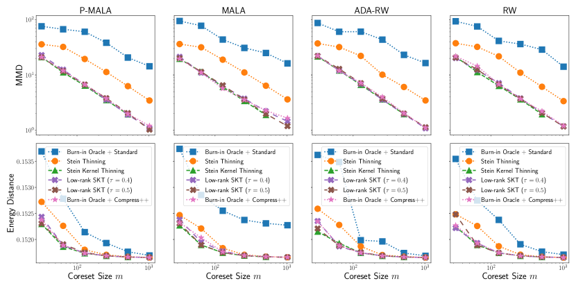
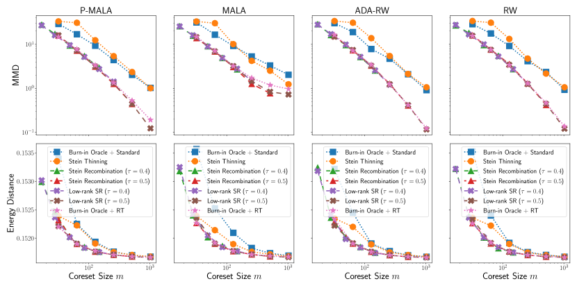
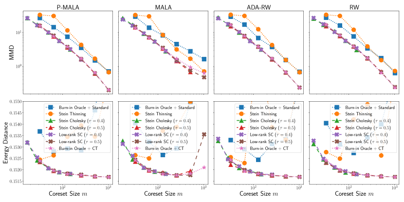
Refer to caption
Figure I.1: Correcting for burn-in with equal-weighted compression. For each of four MCMC algorithms and using only one chain, our methods consistently outperform the Stein and standard thinning baselines and match the 6-chain oracle.
Refer to caption
Figure I.2: Correcting for burn-in with simplex-weighted compression. For each of four MCMC algorithms and using only one chain, our methods consistently outperform the Stein and standard thinning baselines and match the 6-chain oracle.
Refer to caption
Figure I.3: Correcting for burn-in with constant-preserving compression. For each of four MCMC algorithms and using only one chain, our methods consistently outperform the Stein and standard thinning baselines and match the 6-chain oracle.
$\bm{n_{0}}$ ST LD ($0.5$) LD ($0.4$) KT KT-Compress++ RT ($0.5$) RT ($0.4$) CT ($0.5$) CT ($0.4$)
$2^{14}$ 2.50 13.22 12.88 7.31 3.49 0.79 0.60 2.06 1.96
$2^{16}$ 8.48 16.15 15.82 20.77 5.90 2.59 1.68 3.66 3.04
$2^{18}$ 111.06 32.14 20.60 193.03 11.73 11.16 2.63 6.48 3.67
$2^{20}$ - 314.67 131.31 - 35.99 113.71 11.06 51.14 8.42
Table I.1: Breakdown of runtime (in seconds) for the burn-in correction experiment $(d=4)$ of Sec. 5. $n_{0}$ is the input size after standard thinning from the length $n=2\times 10^{6}$ chain (Rem. 2). Each runtime is the median of 3 runs. KT and KT-Compress++ output $m=\sqrt{n_{0}}$ equal-weighted points. RT and CT respectively output $m=n_{0}^{\tau}$ points with simplex or constant-preserving weights for $\tau$ shown in parentheses. In addition, LD, RT, and CT use the rank $n_{0}^{\tau}$. ST and KT took longer than 30 minutes for $n_{0}=2^{20}$ and hence their numbers are not reported.

I.4 Correcting for approximate MCMC details

Surrogate ground truth   Following Liu and Lee [2017], we took the first 10,000 data points and generated $2^{20}$ surrogate ground truth sample points using NUTS [Hoffman et al., 2014] for the evaluation. To generate the surrogate ground truth using NUTS, we used numpyro [Phan et al., 2019]. It took $12$ hours to generate the surrogate ground truth points using the GPU implementation, and we estimate it would have taken $200$ hours using the CPU implementation.

SGFS   For SGFS, we used batch size 32 and the step size schedule $\eta/(1+t)^{0.55}$ where $t$ is the step count and $\eta$ is the initial step size. We chose $\eta$ from $\{10.0,5.0,1.0,0.5,0.1,0.05,0.01\}$, found $\eta=1.0$ gave the best standard thinning MMD to get a coreset size of $m=2^{10}$ , and hence we fixed $\eta=1.0$ in all experiments. We used the version of SGFS [Ahn et al., 2012, SGFS-f] that involves inversion of $d\times d$ matrices — we found the faster version (SGFS-d) that inverts only the diagonal resulted in significantly worse mixing. We implemented SGFS in numpy and ran it on the CPU.

Runtime   The SGFS chain of length $2^{24}$ took approximately 2 hours to generate using the CPU. Remarkably, all of our low-rank methods finish within 10 minutes for $n_{0}=2^{20}$, which is orders of magnitude faster than the time taken to generate the NUTS surrogate ground truth.

Additional results   In Fig. I.4, we plot the posterior mean mean-squared error (MSE) for each compression method in the approximate MCMC experiment of Sec. 5.

Refer to caption
Refer to caption
Refer to caption
Figure I.4: Posterior mean mean-squared error (MSE) for the approximate MCMC compression experiment of Sec. 5. MSE is computed as $\|{\hat{\mathbb{E}}_{\mathbb{P}}Z-\sum_{i\in[n_{0}]}w_{i}x_{i}}\|_{M}^{2}/d$ where $\hat{\mathbb{E}}_{\mathbb{P}}Z$ is the mean of the surrogate ground truth NUTS sample.

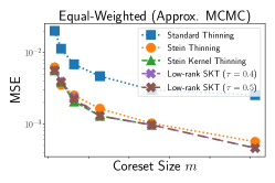
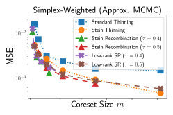
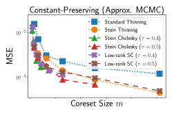
I.5 Correcting for tempering details

In the data release of Riabiz et al. [2020], we noticed there were 349 sample points for which the provided scores were NaNs, so we removed those points at the recommendation of the authors.