A New Computational Method for Energetic Particle Acceleration and Transport with its Feedback

Abstract

We have developed a new computational method to explore astrophysical and heliophysical phenomena, especially those considerably influenced by non-thermal energetic particles. This novel approach considers the backreaction from these energetic particles by incorporating the non-thermal fluid pressure into Magnetohydrodynamics (MHD) equations. The pressure of the non-thermal fluid is evaluated from the energetic particle distribution evolved through Parker’s transport equation, which is solved using stochastic differential equations. We implement this method in the HOW-MHD code (Seo & Ryu 2023), which achieves 5th-order accuracy. We find that without spatial diffusion, the method accurately reproduces the Riemann solution in the hydrodynamic shock tube test when including the non-thermal pressure. Solving Parker’s transport equation allows the determination of pressure terms for both relativistic and non-relativistic non-thermal fluids with adiabatic indices $\gamma_{\rm{NT}}=4/3$ and $\gamma_{\rm{NT}}=5/3$, respectively. The method also successfully replicates the Magnetohydrodynamic shock tube test with non-thermal pressure, successfully resolving the discontinuities within a few cells. Introducing spatial diffusion of non-thermal particles leads to marginal changes in the shock but smooths the contact discontinuity. Importantly, this method successfully simulates the energy spectrum of the non-thermal particles accelerated through shock, which includes feedback from the non-thermal population. These results demonstrate that this method is very powerful for studying particle acceleration when a significant portion of the plasma energy is taken by energetic particles.

1 Introduction

Energetic charged particles exist in a large number of astrophysical and heliophysical systems. These particles gain energy through non-thermal acceleration processes, such as those occurring at collisionless shocks (Bell, 1978; Blandford & Eichler, 1987), magnetohydrodynamic (MHD) turbulence (Petrosian, 2012; Ohira, 2013; Comisso & Sironi, 2018), relativistic shearing flows (Webb et al., 2018; Sironi et al., 2021; Wang et al., 2021), and magnetic reconnection (Guo et al., 2014a; Li et al., 2018, 2022; Guo et al., 2023). In many astrophysical and heliosphysical phenomena, the energetic particle population constitutes a significant fraction of the total energy, for instance, in the loop-top regions of solar flares (Krucker et al., 2010; Oka et al., 2013), supernova remnants (Chevalier, 1983; Bell et al., 2013; Cristofari et al., 2021), and the reconnection region in the Earth’s magnetotail (Oka et al., 2023).

The investigation of particle acceleration employs various methods, with the most well-known being the particle-in-cell (PIC) method. This method, based on the first principles (Dawson, 1983), utilizes Lagrangian macro-particles evolved using fields that are solved using the Eulerian method. The PIC method has been very useful for understanding particle acceleration in various astrophysical phenomena, including shock acceleration (Guo et al., 2014b, c; Ha et al., 2021) and acceleration in the magnetic reconnection region (Drake et al., 2006; Oka et al., 2010; Li et al., 2017, 2019; Zhang et al., 2021; Guo et al., 2015, 2021). However, the PIC method needs to resolve the electron kinetic scales, such as the skin depth for the spatial scale and the inverse of the plasma frequency for the time scale, making it prohibitively challenging for large-scale problems (e.g., solar flare regions are $>10^{9}$ times of electron kinetic scales). To overcome this limitation, the hybrid-PIC method has been developed (Giacalone et al., 1992; Guo & Giacalone, 2013; Haggerty & Caprioli, 2020; Winske et al., 2023; Le et al., 2023; Zhang et al., 2024). This approach treats electrons as a fluid, and solves the kinetic motion of ions, so it only needs to resolve ion kinetic scales. Although this method expands the dynamical scale of kinetic simulations, its domain size is still limited by several thousand ion inertial lengths.

The Monte-Carlo method is widely employed for studying particle acceleration on a hydrodynamic scale. This method directly follows the transport of macro-particles in the background fluid with a particle scattering model. Different scattering methods have been implemented. For instance, one can assume isotropic scattering of the particles in the fluid rest frame (Ellison & Eichler, 1984; Ostrowski, 1998; Ohira, 2013; Kimura et al., 2018; Seo et al., 2023) or include pitch angle scattering (Ellison et al., 1990, 2013). The latter approaches, including Bohm scattering or scattering in Kolmogorov MHD turbulence (Ohira, 2013; Kimura et al., 2018; Seo et al., 2023), treats the mean free path as a function of the momentum of the particles. The Monte-Carlo method has been used to study particle acceleration in various astrophysical phenomena, including shock acceleration (Ellison & Eichler, 1984; Ellison et al., 1990, 1995, 2013), turbulence shear acceleration (Ohira, 2013), and shear acceleration (Ostrowski, 1998). Seo et al. (2023) utilized this method to simulate particle acceleration in radio galaxy jets, discussing the acceleration processes in complex flows that include shocks, shear, and turbulence.

The Parker’s transport equation that describes the transport and acceleration of particles (Parker, 1965; Blandford & Eichler, 1987; Zank, 2014). Traditionally, this equation has been solved using the finite difference method (Jokipii & Kopriva, 1979; Potgieter & Moraal, 1985; Burger & Hattingh, 1995). Recently, the stochastic differential equation method has been widely adopted to solve the transport equation (Zhang, 1999; Florinski & Pogorelov, 2009; Pei et al., 2010; Kong et al., 2017; Li et al., 2018). This equation has been used to understand energetic particles in the outer heliosphere (Florinski & Pogorelov, 2009), at coronal shocks (Kong et al., 2017), in low-$\beta$ magnetic reconnection regions (Li et al., 2018), and in solar flare regions (Kong et al., 2019; Li et al., 2022). While this approach offers robustness and the possibility of adopting anisotropic spatial diffusion (Giacalone & Jokipii, 1999), previous studies have not accounted for the feedback of non-thermal fluid on MHD fluid.

There are several approaches to incorporate the feedback of non-thermal fluid at the hydrodynamic scale (see Ruszkowski & Pfrommer, 2023, for a review). A popular approach is to consider a pressure term from an energetic particle fluid equation. Recently, more sophisticated particle dynamics and feedback are included. The $\it{kglobal}$ model (Drake et al., 2019; Arnold et al., 2021) involves the conservation equation for the guiding center of energetic particles into MHD equations. It is capable of addressing the effects of the instabilities (e.g., firehose instability) driven by the anisotropic pressure of energetic particles. However, its current approach does not include the scattering of energetic particles. The MHD-PIC method (Bai et al., 2015) incorporates the backreaction of Lorentz force from Lagrangian cosmic ray particles into fluid momentum and energy. This approach needs to resolve the gyromotion scale of energetic particles. Another approach involves solving MHD equations that include the energetic particle pressure, obtained from solving the Fokker-Planck equation (Kang & Jones, 2007) or hydrodynamic equation for non-thermal fluid (Kudoh & Hanawa, 2016). These methods take into account the force from energetic particles, such as the force resulting from the pressure gradient of the non-thermal fluid (Kang & Jones, 2007; Kudoh & Hanawa, 2016; Drake et al., 2019), or the Lorentz force of individual particles obtained from the background field (Bai et al., 2015).

In this study, we introduce a method for an MHD simulation that incorporates feedback from the pressure of non-thermal fluid, which is obtained by solving the Parker equation. This method satisfies the Riemann solution, making it applicable on a large dynamic scale with non-thermal fluid feedback. For instance, it can be applied to study magnetic reconnection and associated particle acceleration in solar flares and pickup ion dynamics in the outer heliosphere. Additionally, this method also tracks the energy distribution of energetic particles.

The paper is organized as follows: Section 2 introduces the numerical method, and test results are presented in Section 3. A brief summary and outlook follow in Section 4.

2 Numerical Method

The classical MHD momentum conservation equation is given as,

$$\frac{\partial\rho\mathbf{v}}{\partial t}+\nabla\cdot\left(\rho\mathbf{v}\mathbf{v}+P^{*}\mathbf{I}\right)-\mathbf{J}_{\rm{tot}}\times\mathbf{B}/c=0,$$ (1)

where $\rho$, $\mathbf{v}$, $\mathbf{B}$, $P^{*}$, and $c$ represent density, velocity, magnetic field, the sum of plasma and magnetic pressure given as $P^{*}=P_{g}+B^{2}/2$, and speed of light, respectively. In this context, subscript $g$ refers to the thermal plasma gas. The total current, $\mathbf{J}_{\rm{tot}}$, includes the current from both thermal and non-thermal plasma $\mathbf{J}_{\rm{tot}}=\mathbf{J}_{T}+\mathbf{J}_{\rm{NT}}$. The subscript $\rm NT$ denotes the non-thermal plasma. Some studies directly compensate current of non-thermal fluid (Bai et al., 2015), whereas we consider the non-thermal component as a “non-thermal fluid” and the force density on the thermal plasma. For non-thermal fluid, the force density is given as (Drake et al., 2019),

$$\mathbf{F_{\rm{NT}}}=-n_{\rm{NT}}\mathcal{E}-n_{\rm{NT}}\mathbf{u_{\rm{NT}}}\times\mathbf{B}/c-\nabla\cdot P_{\rm{NT}}\mathbf{I},$$ (2)

where $n_{\rm{NT}}$ is the charge density of the non-thermal fluid, $\mathbf{u_{\rm{NT}}}$ is the bulk velocity of the non-thermal fluid, $P_{\rm{\rm{NT}}}$ is the pressure of the non-thermal fluid, given by the mean momentum of the non-thermal fluid (Drake et al., 2019), and $\mathcal{E}$ is the electric field. In our simulations, we assumed nearly isotropic distribution of the non-thermal fluid momentum, $p_{\rm NT}$; hence, the pressure of the non-thermal fluid is given by (Kudoh & Hanawa, 2016),

$$P_{\rm{NT}}=(\gamma_{\rm{NT}}-1)E_{\rm{NT}}.$$ (3)

where $\gamma_{\rm{NT}}$ is the adiabatic index for the non-thermal fluid. $E_{\rm{NT}}$ is the energy density of the non-thermal fluid. $\mathcal{E}$ is given as MHD Ohm’s law term and Hall term of non-thermal fluid (Bai et al., 2015),

$$\mathcal{E}=-\frac{\mathbf{v}}{c}\times\mathbf{B}-\frac{n_{\rm{\rm{NT}}}}{|n_{e}|}\frac{(\mathbf{u_{\rm{NT}}}-\mathbf{v})}{c}\times\mathbf{B}.$$ (4)

where $n_{e}$ are the charge densities of electrons. Since the bulk motion of the non-thermal fluid is caused by the advection through thermal fluid motion, the velocity of the bulk motion is almost the same as the plasma velocity, $\mathbf{u_{\rm{NT}}}\approx\mathbf{v}$, then equation (2) is given as,

$$\mathbf{F_{\rm{NT}}}=-\nabla\cdot P_{\rm{NT}}\mathbf{I}$$ (5)

Therefore, resistive MHD equations with non-thermal fluid feedback are given as,

$$\frac{\partial\rho}{\partial t}+\nabla\cdot(\rho\mathbf{v})=0$$ (6)

$$\frac{\partial\rho\mathbf{v}}{\partial t}+\nabla\cdot\left(\rho\mathbf{v}\mathbf{v}+P^{*}\mathbf{I}-\mathbf{B}\mathbf{B}\right)=-\nabla\cdot P_{\rm{NT}}\mathbf{I}$$ (7)

$$\frac{\partial E}{\partial t}+\nabla\cdot\left[(E+P^{*})\mathbf{v}-\mathbf{B}(\mathbf{B}\cdot\mathbf{v})\right]=\nabla\cdot(\mathbf{B}\times\eta\mathbf{j})-\mathbf{v}\cdot(\nabla\cdot P_{\rm{NT}}\mathbf{I})$$ (8)

$$\frac{\partial\mathbf{B}}{\partial t}-\nabla\times(\mathbf{v}\times\mathbf{B})=\eta\nabla^{2}\mathbf{B}$$ (9)

where the total energy density excluding the energy of the non-thermal energetic particles is given as $E=P_{g}/(\gamma_{g}-1)+(\rho v^{2}+B^{2})/2$, where $v^{2}=v_{x}^{2}+v_{y}^{2}+v_{z}^{2}$ and $B^{2}=B_{x}^{2}+B_{y}^{2}+B_{z}^{2}$, and $\gamma_{g}$ and $\eta$ are the adiabatic index of the thermal plasma and resistivity, respectively. Equation (7) is identical to equation (6) in Drake et al. (2019) assuming the pressure is isotropic. When we determine the total pressure as $P_{\rm{tot}}=P^{*}+P_{\rm{NT}}$, equations (6) - (9) are identical to the resistive single fluid MHD equations. The physical significance of these equations lies in solving the MHD equation while including non-thermal fluid pressure (Kang & Jones, 2007; Kudoh & Hanawa, 2016).

To solve the MHD equations, we utilize the HOW-MHD code (Seo & Ryu, 2023), which employs finite difference fifth-order Weighted Essentially Non-Oscillatory (WENO) reconstruction and a fourth-order Strong-Stability-Preserving Runge-Kutta (SSPRK) method with a high-order constrained flux algorithm. This code has a high effective resolution, allowing it to provide detailed non-linear structures such as shocks and turbulence, which are important for tracking the acceleration process at sharp MHD structures.

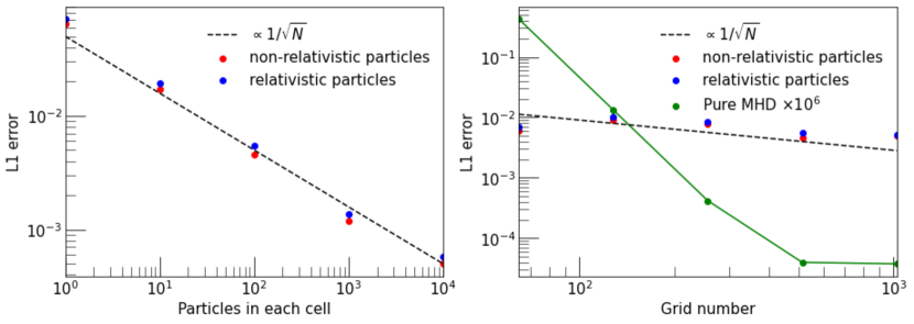
Figure 1: (Left) L1 error dependency on the number of particles per cell. The red and blue dots indicate particles in the non-relativistic and relativistic regimes, respectively. The black dashed line indicates the inverse proportionality to the square root of the total number of particles. (Right) L1 error dependency on grid resolution. The color code is the same as in the left panel. The green solid line indicates the L1 error of pure MHD simulation.

To obtain the distribution of the non-thermal fluid, we solve Parker’s transport equation for non-thermal fluid, as follows,

$$\frac{\partial f}{\partial t}+(\mathbf{v}+\mathbf{v_{d}})\cdot\nabla f-\frac{1}{3}\nabla\cdot\mathbf{v}\frac{\partial f}{\partial\ln p_{\rm{NT}}}=\nabla\cdot(\boldsymbol{\kappa}\nabla f)+Q$$ (10)

where $f(x_{\rm{NT}},p_{\rm{NT}},t)$ is the distribution function, which is function of position, $x_{\rm{NT}}$, specific momentum, $p_{\rm{NT}}$, and time, $t$. $\mathbf{v_{d}}$, $\boldsymbol{\kappa}$, and $Q$ are the particle drift velocity, the spatial diffusion tensor, and the source term, respectively. Here, we have assumed a nearly isotropic momentum distribution. The spatial diffusion coefficient, $\boldsymbol{\kappa}$, is defined based on the specific problem being solved, such as diffusion in MHD turbulence (Giacalone & Jokipii, 1999) or Bohm diffusion near the shock (Kang & Jones, 2007).

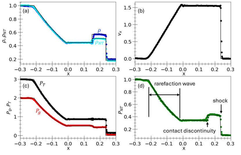
Figure 2: 2D hydrodynamic shock tube with relativistic non-thermal fluid simulation results for (a) density of the plasma (blue dot) and non-thermal fluid (cyan dot), (b) $v_{x}$, (c) thermal plasma pressure (red dot) and total pressure (black dot), and (d) non-thermal fluid pressure at $t$=0.1. Solid black lines indicate the analytic Riemann solution.

To solve Parker’s transport equation, we solve its Fokker-Planck form expressed for $F=fp_{\rm{NT}}^{2}$ while assuming the neglect of the source term $Q$ (Zhang, 1999; Florinski & Pogorelov, 2009; Pei et al., 2010; Kong et al., 2017; Li et al., 2018),

$$\frac{\partial F}{\partial t}=-\nabla\cdot[(\nabla\cdot\boldsymbol{\kappa+\mathbf{v}})F]+\frac{\partial}{\partial p_{\rm{NT}}}\left[\frac{p_{\rm{NT}}}{3}\nabla\cdot\mathbf{v}F\right]+\nabla\cdot(\nabla\cdot(\boldsymbol{\kappa}F))$$ (11)

This equation can be expressed as Ito-type stochastic differential equations, as follows,

$$dX=(\nabla\cdot\boldsymbol{\kappa}+\mathbf{v})ds+\sum_{\sigma}\alpha_{\sigma}dW_{\sigma}(s),$$ (12)

$$dp_{\rm{NT}}=-\frac{p_{\rm{NT}}}{3}(\nabla\cdot\mathbf{v})ds,$$ (13)

where $\sum_{\sigma}\alpha^{\mu}_{\sigma}\alpha^{\nu}_{\sigma}=2\kappa^{\mu\nu}$, the term $dW$ represents the normalized distributed random number with mean zero and variance $\sqrt{\Delta t_{\rm{SDE}}}$, where $\Delta t_{\rm{SDE}}$ is the time step for stochastic integration. We use linear interpolation for 1D simulation, bilinear interpolation for 2D simulation, and trilinear interpolation for 3D simulation to obtain the primitive variables at a specific point. The details of the method used to solve stochastic differential equations can be found in Li et al. (2018). The spatial diffusion coefficient is determined by the problem being solved. The energy density of the non-thermal fluid is calculated by the averaging of the specific momentum within the grid and density of the non-thermal fluid, $\rho_{\rm{NT}}$. For relativistic non-thermal fluid, $\gamma_{\rm{NT}}=4/3$ and,

$$E_{\rm{NT}}=\rho_{\rm{NT}}\left<p_{\rm{NT}}\right>c.$$ (14)

For non-relativistic non-thermal fluid, $\gamma_{\rm{NT}}=5/3$ and,

$$E_{\rm{NT}}=\frac{1}{2}\rho_{\rm{NT}}\left<p_{\rm{NT}}^{2}\right>.$$ (15)

To achieve a high-order of accuracy in this code, we adopt a high-order difference method to obtain divergence and non-thermal fluid pressure (Romão et al., 2012),

$$\frac{\partial Q}{\partial x}=\frac{aQ_{i+3}-bQ_{i+2}+cQ_{i+1}-cQ_{i-1}+bQ_{i-2}-aQ_{i-3}}{d\Delta x},$$ (16)

where $Q$ is an arbitrary function and $i$ is the number of the grid along the $x$ direction. In Equation (16), we omitted the $y$ and $z$ directions for simplification. For a fourth-order difference, $a=0$, $b=1$, $c=8$, and $d=12$, and for a sixth-order difference, $a=1$, $b=9$, $c=45$, and $d=60$. As shown in the pressure balance test, this method suppresses spurious oscillations (see section 3.4).

3 Test problems

To ensure proper demonstration of the cosmic ray pressure obtained from the Parker equation and its adequate feedback in the hydrodynamic regime, we benchmark the shock tube test using non-thermal fluid pressures as suggested in Kudoh & Hanawa (2016). We denote primitive variables as $\mathbf{u}=(\rho,v_{x},P_{g},P_{\rm{NT}})$ for the hydrodynamic shock tube test in 3.2 and the pressure balance mode in 3.4, and $\mathbf{u}=(\rho,v_{x},v_{y},v_{z},B_{x},B_{y},B_{z},P_{g},P_{\rm{NT}})$ for the magnetohydrodynamic shock tube test in section 3.3 and reflection shock test in section 3.5. All tests adopt a Courant-Friedrichs-Lewy number of 1.5, leveraging the advantages of SSPRK (Seo & Ryu, 2023). The MHD time step, $\Delta t$, is determined by the maximum eigenvalues within the domain and grid resolution (see Seo & Ryu, 2023, for details).

3.1 Advection of entropy wave

Solving SDE involves using the Lagrangian method, which generates random errors. To estimate the effect of this error, we conduct an advection of entropy wave test. This test is performed in 1D, with density perturbation given by,

$$\rho_{g}=\rho_{0}+\epsilon_{\rho}\sin\left(\frac{2\pi}{L}\right),$$ (17)

where $L=1$ is the domain size, $\rho_{0}=1$, and $\epsilon_{\rho}=0.1$. The other parameters are set as follows: $P_{g}=1$, $P_{\rm{NT}}=1$, and $v_{x}=10$, with no magnetic field and no spatial diffusion, $\kappa_{\perp}=\kappa_{\parallel}=0$. The L1 error is determined as,

$$\text{L1 error}=\sqrt{\sum_{s=1}^{5}\left(\sum_{i}\frac{|\mathbf{u}_{i}^{s}(t)-\mathbf{u}_{i}^{s}(0)|}{N}\right)},$$ (18)

where $N$ is the number of grid points, $i$ is the cell position, and $s$ is the component of the primitive variables. For the test on the dependency of the number of particles per cell, we use 512 grid points, and for the test on the dependency of the grid number, we put 100 particles in each cell. As shown in the left panel of Figure 1, the random error decreases with the square root of the number of particles per cell, $\sqrt{N_{p}}$, as expected. The L1 error for 1000 particles per cell is approximately $1\%$ of the density perturbation. In this limit, the random error has a marginal effect on the wave. Hence, while a low number of particles can distort the hydrodynamic structures, a sufficiently large number of particles can minimize this effect. The L1 error of pure MHD is much less than the error from SDE (as shown by the solid green line in the right panel of Figure 1; this error saturates in the double-precision limit). Increasing the grid number increases the total number of particles, so the L1 error also decreases with $\sqrt{N_{p}}$. This pattern indicates that the random error when using the Lagrangian method to solve SDE is much larger than those caused by numerical dissipation.

3.2 Hydrodynamic shock

The first test is a simple hydrodynamic shock tube, initially containing high-density and high-pressure fluid on one side, and low-density and low-pressure fluid on the other. The initial conditions are specified as follows: for the left side, $\mathbf{u}_{L}=(1.0,0.0,2.0,1.0)$, and for the right side, $\mathbf{u}_{R}=(0.2,0.0,0.02,P_{\rm{NT,2}})$. Where $P_{\rm{NT,2}}=0.1$ for relativistic non-thermal fluid and $P_{\rm{NT,2}}=0.06$ for non-relativistic non-thermal fluid. The initial density of the non-thermal fluid is determined by the adiabatic condition, $\rho_{\rm{NT}}=\rho_{\rm{NT},0}P_{\rm{NT}}^{1/\gamma_{\rm{NT}}}$, where $\rho_{\rm{NT},0}=1$ for this simulation. In this test, we adopt relativistic non-thermal fluid, with the pressure given by equation (14). The domain is $[-0.5,0.5]\times[-0.25,0.25]$ with a grid resolution of $512\times 256$. We inject 1,000 pseudo-particles into each cell to solve the SDE. The test results are presented in Figure 2 at $t$=0.1. In this figure, we averaged the primitive variables along the $y$-axis to reduce the random noise. In this test, spatial diffusion is not included to allow for direct comparison with the shock tube test of Kudoh & Hanawa (2016), but we have adopted spatial diffusion in the MHD shock tube (section 3.3) and reflecting shock (section 3.5).

As shown in Figure 2, an expansion wave ($x$=-0.23 to -0.02), a contact discontinuity ($x$=0.14), and a shock ($x$=0.24) are generated. Thanks to the high-order WENO Reconstruction in the HOW-MHD code, the contact discontinuity and shock are resolved within approximately 3-4 cells. The non-thermal fluid pressure, $P_{\rm{NT}}$, is obtained by solving equation (11), as illustrated by the green dot in the bottom-right plot of Figure 2. The solution is well aligned with the analytic Riemann solution provided in Kudoh & Hanawa (2016). This result demonstrates that solving the SDE can provide proper non-thermal fluid pressure and adequate feedback in the hydrodynamic regime. At the contact discontinuity, small spurious oscillations are generated, resulting in approximately a 2% error in total pressure. This error is primarily due to the numerical dissipation of the non-thermal fluid (see section 3.4).

We performed an additional test for the non-relativistic non-thermal fluid, using the pressure given by equation (15). The initial conditions are the same as in the first simulation, but the initial density of the non-thermal fluid is determined by the adiabatic condition with $\gamma_{\rm{NT}}=5/3$. Consequently, the initial density of the non-thermal fluid on the right side is larger than in the previous test. The test results are presented in Figure 3.

For the non-relativistic non-thermal fluid, the reduction in non-thermal fluid energy ($E_{\rm{NT}}=P_{\rm{NT}}/(\gamma_{\rm{NT}}-1)$) results in a reduced compression at the shock. This leads to a decrease in the jump of the plasma density, pressure, and velocity of the downstream of the shock (see $x$=0.2-0.3 in Figures 2 and 3). However, since the non-thermal fluid pressure is given as $P_{\rm{NT}}=\rho_{\rm{NT}}^{\gamma_{\rm{NT}}}$, the non-thermal fluid pressure in the shock downstream region is larger than in the relativistic case, even though the compression is reduced. This test demonstrates that our method also works well within the non-relativistic non-thermal fluid limit.

3.3 Magnetohydrodynamic shock

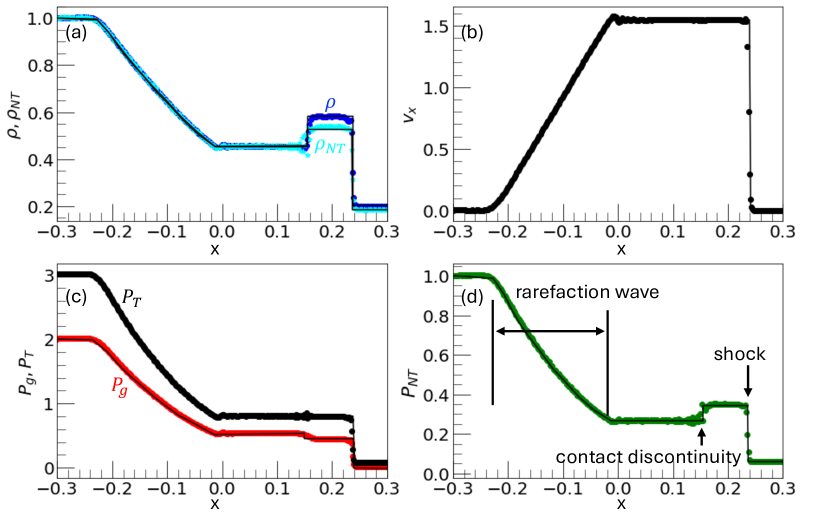
Figure 3: 2D hydrodynamic shock tube with non-relativistic non-thermal fluid simulation results for (a) density of the plasma (blue dot) and non-thermal fluid (cyan dot), (b) $v_{x}$, (c) thermal plasma pressure (red dot) and total pressure (black dot), and (d) non-thermal fluid pressure at $t$=0.1. Solid black lines indicate the analytic Riemann solution.

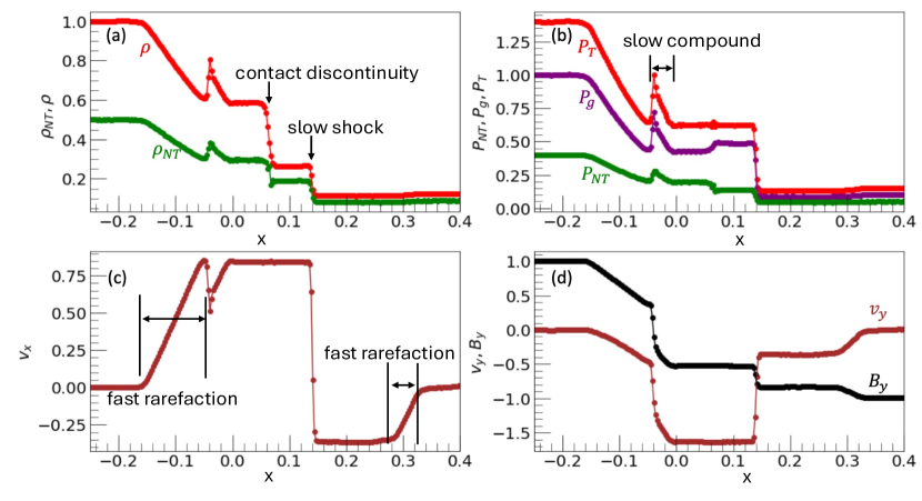
Figure 4: 2D magentohydrodynamic shock tube with relativistic non-thermal fluid simulation results for (a) density of the plasma (red dot) and non-thermal fluid (green dot), (b) total pressure (red dot), thermal plasma pressure (purple dot), and non-thermal fluid pressure (green dot), (c) $v_{x}$, and (d) non-thermal fluid pressure at $t$=0.08.

To use this method in MHD simulations, we conduct the Brio-Wu shock tube test (Brio & Wu, 1988) with relativistic non-thermal fluid, following the approach outlined in Kudoh & Hanawa (2016). In all MHD test simulation, $\eta=0$. The initial conditions for the left side are given as $\mathbf{u}_{L}=(1.0,0.0,0.0,0.0,1.0,1.0,0.0,1.0,0.4)$, and for the right side, $\mathbf{u}_{R}=(0.125,0.0,0.0,0.0,1.0,-1.0,0.0,0.1,0.04)$. The simulation end time is $t=0.08$. The domain size and the number of injection pseudo-particles are the same as in the hydrodynamic shock tube test. Figure 4 shows that this test generates fast rarefaction, slow compound, contact discontinuity, slow shock, and fast rarefaction, from left to right. For the first approach, we do not adopt spatial diffusion. As shown in Figure 4, our result agrees well with the result of Kudoh & Hanawa (2016), for instance, the position and amplitude of the MHD structures (see Figure 11 in Kudoh & Hanawa (2016)). Especially, our code captures the contact discontinuity within 3-4 cells.

For the next test, we incorporate spatial diffusion using two scattering models. The first model is the Bohm-like diffusion model, $\kappa_{\parallel}=\kappa_{0}(p_{\rm{NT}}/p_{0})$ (Kang & Jones, 2007), and the second model is the Kolmogorov scattering model, $\kappa_{\parallel}=\kappa_{0}(p_{\rm{NT}}/p_{0})^{4/3}$ (Li et al., 2018). Additionally, we examine the $\kappa_{\perp}/\kappa_{\parallel}$ dependence. In this simulation, we set $\kappa_{0}=0.003$. We present the diffusion dependence test in Figure 5, with a particular focus on the right fast rarefaction (panel (a) in Figure 5), contact discontinuity, and slow shock (panels (b)-(d) in Figure 5).

As expected from the model, the spatial diffusion coefficient is larger for the Kolmogorov scattering model at the same momentum. Consequently, more diffusion of the structures is observed in the Kolmogorov scattering model for rarefaction and discontinuity than in the Bohm diffusion model, but the difference is marginal. With non-zero $B_{y}$ (see black line in Figure 4 (d)), a lower $\kappa_{\perp}/\kappa_{\parallel}$ leads to a smaller $\kappa_{xx}$ and, consequently, less spatial diffusion when $\kappa_{\perp}/\kappa_{\parallel}=0.01$ than when it is 1. A $\kappa_{\perp}/\kappa_{\parallel}$ value of 1 indicates significant diffusion of non-thermal fluid perpendicular to the magnetic field direction, leading to increased diffusion in both structures. Compared to the rarefaction, spatial diffusion of non-thermal fluid does not smooth the shock as much because of its large compression.

A contact discontinuity is noticeable around $x=0.07$ in panels (b)-(d) of Figure 5. As mentioned earlier, without spatial diffusion, spurious oscillations occur around the contact discontinuity. However, when including spatial diffusion, these oscillations disappear, and sharp boundaries become continuous structures. Due to the diffusion of these particles, non-thermal fluid density and pressure are slightly increased. However, total pressure is preserved, as shown in panel (d) of Figure 5. Since the shock Mach number is determined by the total pressure jump, spatial diffusion does not affect the strength of the shock.

In summary, spatial diffusion of the non-thermal fluid can smooth out MHD structures, such as contact discontinuities or rarefactions, but it only has a marginal effect that cannot significantly distort the MHD structure.

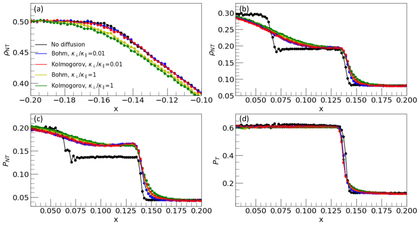
Figure 5: The 2D magnetohydrodynamic shock tube with relativistic non-thermal fluid simulation yields results at $t=0.08$ for (a) non-thermal fluid density in the rarefaction range, (b) non-thermal fluid density in the contact discontinuity and slow shock, (c) non-thermal fluid pressure in the same range, and (d) total pressure in the same range. The color code depends on the scattering model and spatial diffusion coefficient as follows: no spatial diffusion (black), Bohm diffusion with $\kappa_{\perp}/\kappa_{\parallel}=0.01$ (blue), Kolmogorov scattering with $\kappa_{\perp}/\kappa_{\parallel}=0.01$ (red), Bohm diffusion with $\kappa_{\perp}/\kappa_{\parallel}=1$ (yellow), and Kolmogorov scattering with $\kappa_{\perp}/\kappa_{\parallel}=1$ (green).

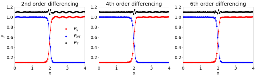
Figure 6: The Advection of the Pressure Balance Mode test at $t=2$ with (left) 2nd, (middle) 4th, and (right) 6th order differencing method (equation (16)). Red dot indicates the plasma pressure profile, blue dot indicates the non-thermal fluid pressure, and black dot indicates the total pressure.

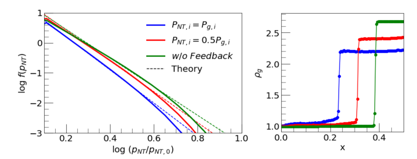
Figure 7: (Left) The energy spectrum of non-thermal fluid at $t=0.5$ with $P_{\rm{NT},i}=1P_{g,i}$ (blue solid), $P_{\rm{NT},i}=0.5P_{g,i}$ (red solid), and $P_{\rm{NT},i}=0P_{g,i}$ (green solid). The dashed lines represent the analytic solutions for the respective shock compression ratios. (Right) The density profile around the shock region at $t=0.5$. The color code used is the same as in the left panel.

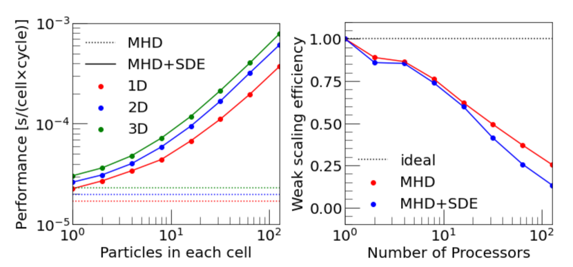
Figure 8: (Left) Computational performance versus the number of particles per cell, which is defined as the computational time divided by the total number of cells and the number of MHD cycles. Red, blue, and green colors indicate tests performed in 1D, 2D, and 3D, respectively. The dashed lines represent the performance with only solving MHD, with the dimension indicated by the respective color code. (Right) Weak scaling comparison between only MHD (red) and MHD with the SDE method (blue).

3.4 Advection of the Pressure Balance Mode

The advection of the pressure balance mode can generate unphysical structures, as reported in Kudoh & Hanawa (2016). The initial condition of the test for the left side is $\mathbf{u}_{L}=(1.0,1.0,0.1,1.0)$, and for the right side is $\mathbf{u}_{R}=(1.0,1.0,1.0,0.1)$. The simulation end time is $t=2$. This test is conducted in 1D with a spatial grid spacing of $\Delta x=0.1$. According to Kudoh & Hanawa (2016), the numerical diffusion of non-thermal fluid density leads to an energy loss, hence generating spurious structures. As shown by the black dots in Figure 6, which indicate the total pressure, spurious structures are also found at the discontinuity region due to numerical diffusion. Although we obtain the evolution of the non-thermal fluid pressure by SDE, this structure does not propagate. Additionally, due to the high-order accuracy of the HOW-MHD code, adopting low-order differencing in calculating the gradient of non-thermal fluid pressure generates oscillations at the discontinuity of thermal and non-thermal fluid pressure (see the left panel of Figure 6). This occurs due to a mismatch between the spatial accuracy and the accuracy of the non-thermal fluid pressure gradient. As shown in Figure 6, when implementing high-order differencing, these oscillations are almost suppressed. Hence, we adopt sixth-order differencing as a fiducial scheme.

3.5 The energy spectrum of accelerated particles by diffusive shock acceleration

The strength of solving Parker’s equation lies in its ability to obtain the energy spectrum of non-thermal fluid. To demonstrate the proper occurrence of first-order Fermi particle acceleration, we generate a shock with a reflecting boundary. In this test, we generate a parallel shock, with the initial condition given as $\mathbf{u}=(1.0,2.0,0.0,0.0,1.0,0.0,0.0,1.0,P_{\rm{NT}})$. The grid resolution is 256$\times$128 with a domain of [0,1]$\times$[-0.25,0.25]. The right-side boundary is a reflecting boundary, the left side is an open boundary, and the top and bottom boundaries are periodic boundaries for mimicking an infinite shock size. Non-thermal fluid are contained with 1,000 pseudo-particles in each cell. Isotropic spatial diffusion, $\kappa_{\perp}=\kappa_{\parallel}$, and the Kolmogorov diffusion, $\kappa_{\parallel}=\kappa_{0}(p_{\rm{NT}}/p_{0})^{4/3}(\rho/\rho_{1})^{-1}$, are adopted, where $\kappa_{0}=0.1$ with non-relativistic particles. The density dependence term, $(\rho/\rho_{1})^{-1}$, where $\rho_{1}$ is the upstream plasma density, is adopted to quench the energetic particle acoustic instability in the precursor of shock, which is highly modified by non-thermal energetic particles (Kang & Jones, 2007). We set the non-thermal fluid pressure of three cases as $P_{\rm{NT},i}=0P_{g,i}$, $0.5P_{g,i}$, and $1P_{g,i}$. The case where $P_{\rm{NT},i}=0P_{g,i}$ does not include feedback from the non-thermal fluid. The simulation end time is $t=0.5$. To obtain the proper result in diffusive shock acceleration through SDE, the following two conditions shall be satisfied (Kong et al., 2017): the first condition is $\kappa_{xx}/v_{s}>X_{\rm{sh}}$, where $v_{s}$ and $X_{\rm{sh}}$ are the shock speed and the shock thickness, respectively. The second condition is a small $\Delta t_{\rm{SDE}}$ to capture the transition of the shock. Thus, we adopt the timestep for SDE as $\Delta t_{\rm{SDE}}=10^{-5}(p/p_{0})^{-4/3}$, ensuring satisfaction of this relation. The thickness of exponential decrease, $X_{\rm{exp}}$, is determined as $\kappa_{2}/v_{2}$, where $\kappa_{2}$ and $v_{2}$ are the spatial diffusion coefficient in the downstream and speed of the downstream in the shock rest frame (Zhang, 2000), respectively. Since this value is a few factors larger than the thickness of the shock, $X_{\rm{exp}}>X_{\rm{sh}}$, pre-compression region (see the right panel of Figure 7) is generated in the plasma density profile (Vink, 2020).

As shown in Figure 7, the compression ratio of the shock decreases for the large $P_{\rm{NT},i}$ case. Hence, the energy spectrum of the non-thermal fluid becomes steeper. The dashed line in the left panel of Figure 7 is given as $f(p_{\rm{NT}})\propto p_{\rm{NT}}^{-\frac{3\chi}{\chi-1}}$, where $\chi$ is the compression ratio of the shock. It matches very well with the spectral shape of non-thermal fluid. Even though the Mach number of the shock decreases with increasing $P_{\rm{NT,i}}$, the sound speed of the upstream region increases with increasing $P_{\rm{NT,i}}$, given as $c_{s}=((\gamma_{g}P_{g}+\gamma_{\rm{NT}}P_{\rm{NT}})/\rho)^{0.5}$, so the shock speed in the upstream rest frame increases. This trend is also consistent when $P_{g,i}$ is 1.5 or 2, but without $P_{\rm{NT,i}}$ (not shown here).

3.6 Scaling test

To estimate the computational efficiency of this method, we perform performance tests focusing on the number of particles in each cell and weak scaling. For these tests, we conduct a reflection shock generation test (section 3.6) in 1D to 3D, with a 2D setup selected for the weak scaling test. In the weak scaling test, the number of particles in each cell is fixed to 8. In the left panel of Figure 8, similar to the MHD-PIC method (Sun & Bai, 2023), the computational cost remains relatively flat when the number of particles is less than $\approx 10$, due to constant overhead. Beyond that, the computational cost almost linearly depends on the number of particles in the cell. As shown in the right panel of Figure 8, solving MHD with the SDE method has almost similar efficiency to using only the MHD method.

4 Summary

To investigate astrophysical phenomena containing a large fraction of energetic particles, we have developed a new method for including feedback from non-thermal particles. To solve the distribution of non-thermal component, we employ the stochastic differential equation (Li et al., 2018), assuming isotropic momentum of particles, and obtain their pressure. We incorporate the non-thermal pressure into the MHD equations to apply feedback from the non-thermal fluid. The extended MHD equations are solved using the HOW-MHD code (Seo & Ryu, 2023), providing high-order accuracy. The major features of this method are summarized as follows:

1. Without the spatial diffusion of non-thermal fluid, we obtain the pressure of non-thermal fluid by solving the Stochastic Differential Equation (SDE). This method accurately reproduces the Riemann solution in the hydrodynamic shock tube test when including non-thermal plasma pressure.

2. By solving Parker’s transport equation using SDE, we properly determine the pressures of the relativistic or non-relativistic non-thermal fluid, with adiabatic indices $\gamma_{\rm{NT}}=4/3$ and $\gamma_{\rm{NT}}=5/3$, respectively.

3. This method successfully replicates the Brio-Wu MHD shock tube test with non-thermal fluid pressure, previously studied by Kudoh & Hanawa (2016). Thanks to the high-order accuracy of the MHD code, discontinuities, including contact discontinuity, are resolved within 3-4 cells. When spatial diffusion of non-thermal fluid is introduced, the contact discontinuity can be diffused, but only marginal changes occur in the shock.

4. By solving Parker’s transport equation, we obtain the energy spectrum of non-thermal fluid, successfully describing the analytic solution of first-order Fermi acceleration. This capability allows us to compare simulation data with observational data, such as X-ray emissions produced by non-thermal electrons from flare regions.

In the following study, we will investigate the effect of the feedback of non-thermal fluid in the magnetic reconnection region with various plasma parameters, such as plasma beta and the strength of the guide field. Our aim is to apply this study to understand the acceleration and distribution of energetic particles in shocks, turbulence, and magnetic reconnection occurring within the interstellar medium, intracluster medium, solar wind, heliosheath, and outer heliosphere. In further studies, we plan to solve the focused transport equation (Zank, 2014; le Roux et al., 2015; Zhang & Zhao, 2017; Kong et al., 2022) to address the momentum distribution of energetic particles, which exhibit high anisotropy.

References

- Arnold et al. (2021) Arnold, H., Drake, J. F., Swisdak, M., et al. 2021, Phys. Rev. Lett., 126, 135101, doi: 10.1103/PhysRevLett.126.135101
- Bai et al. (2015) Bai, X.-N., Caprioli, D., Sironi, L., & Spitkovsky, A. 2015, ApJ, 809, 55, doi: 10.1088/0004-637X/809/1/55
- Bell (1978) Bell, A. R. 1978, MNRAS, 182, 147, doi: 10.1093/mnras/182.2.147
- Bell et al. (2013) Bell, A. R., Schure, K. M., Reville, B., & Giacinti, G. 2013, MNRAS, 431, 415, doi: 10.1093/mnras/stt179
- Blandford & Eichler (1987) Blandford, R., & Eichler, D. 1987, Phys. Rep., 154, 1, doi: 10.1016/0370-1573(87)90134-7
- Brio & Wu (1988) Brio, M., & Wu, C. C. 1988, Journal of Computational Physics, 75, 400, doi: 10.1016/0021-9991(88)90120-9
- Burger & Hattingh (1995) Burger, R. A., & Hattingh, M. 1995, Ap&SS, 230, 375, doi: 10.1007/BF00658195
- Chevalier (1983) Chevalier, R. A. 1983, ApJ, 272, 765, doi: 10.1086/161338
- Comisso & Sironi (2018) Comisso, L., & Sironi, L. 2018, Phys. Rev. Lett., 121, 255101, doi: 10.1103/PhysRevLett.121.255101
- Cristofari et al. (2021) Cristofari, P., Blasi, P., & Caprioli, D. 2021, A&A, 650, A62, doi: 10.1051/0004-6361/202140448
- Dawson (1983) Dawson, J. M. 1983, Rev. Mod. Phys., 55, 403, doi: 10.1103/RevModPhys.55.403
- Drake et al. (2006) Drake, J., Swisdak, M., Che, H., & Shay, M. 2006, Nature, 443, 553
- Drake et al. (2019) Drake, J. F., Arnold, H., Swisdak, M., & Dahlin, J. T. 2019, Physics of Plasmas, 26, 012901, doi: 10.1063/1.5058140
- Ellison et al. (1995) Ellison, D. C., Baring, M. G., & Jones, F. C. 1995, ApJ, 453, 873, doi: 10.1086/176447
- Ellison & Eichler (1984) Ellison, D. C., & Eichler, D. 1984, ApJ, 286, 691, doi: 10.1086/162644
- Ellison et al. (1990) Ellison, D. C., Jones, F. C., & Reynolds, S. P. 1990, ApJ, 360, 702, doi: 10.1086/169156
- Ellison et al. (2013) Ellison, D. C., Warren, D. C., & Bykov, A. M. 2013, ApJ, 776, 46, doi: 10.1088/0004-637X/776/1/46
- Florinski & Pogorelov (2009) Florinski, V., & Pogorelov, N. V. 2009, ApJ, 701, 642, doi: 10.1088/0004-637X/701/1/642
- Giacalone et al. (1992) Giacalone, J., Burgess, D., Schwartz, S. J., & Ellison, D. C. 1992, Geophys. Res. Lett., 19, 433, doi: 10.1029/92GL00379
- Giacalone & Jokipii (1999) Giacalone, J., & Jokipii, J. R. 1999, ApJ, 520, 204, doi: 10.1086/307452
- Guo & Giacalone (2013) Guo, F., & Giacalone, J. 2013, ApJ, 773, 158, doi: 10.1088/0004-637X/773/2/158
- Guo et al. (2014a) Guo, F., Li, H., Daughton, W., & Liu, Y.-H. 2014a, Phys. Rev. Lett., 113, 155005, doi: 10.1103/PhysRevLett.113.155005
- Guo et al. (2021) Guo, F., Li, X., Daughton, W., et al. 2021, ApJ, 919, 111, doi: 10.3847/1538-4357/ac0918
- Guo et al. (2015) Guo, F., Liu, Y.-H., Daughton, W., & Li, H. 2015, ApJ, 806, 167, doi: 10.1088/0004-637X/806/2/167
- Guo et al. (2023) Guo, F., Liu, Y.-H., Zenitani, S., & Hoshino, M. 2023, arXiv e-prints, arXiv:2309.13382, doi: 10.48550/arXiv.2309.13382
- Guo et al. (2014b) Guo, X., Sironi, L., & Narayan, R. 2014b, ApJ, 794, 153, doi: 10.1088/0004-637X/794/2/153
- Guo et al. (2014c) —. 2014c, ApJ, 797, 47, doi: 10.1088/0004-637X/797/1/47
- Ha et al. (2021) Ha, J.-H., Kim, S., Ryu, D., & Kang, H. 2021, ApJ, 915, 18, doi: 10.3847/1538-4357/abfb68
- Haggerty & Caprioli (2020) Haggerty, C. C., & Caprioli, D. 2020, ApJ, 905, 1, doi: 10.3847/1538-4357/abbe06
- Jokipii & Kopriva (1979) Jokipii, J. R., & Kopriva, D. A. 1979, ApJ, 234, 384, doi: 10.1086/157506
- Kang & Jones (2007) Kang, H., & Jones, T. W. 2007, Astroparticle Physics, 28, 232, doi: 10.1016/j.astropartphys.2007.05.007
- Kimura et al. (2018) Kimura, S. S., Murase, K., & Zhang, B. T. 2018, Phys. Rev. D, 97, 023026, doi: 10.1103/PhysRevD.97.023026
- Kong et al. (2017) Kong, X., Guo, F., Giacalone, J., Li, H., & Chen, Y. 2017, ApJ, 851, 38, doi: 10.3847/1538-4357/aa97d7
- Kong et al. (2019) Kong, X., Guo, F., Shen, C., et al. 2019, ApJ, 887, L37, doi: 10.3847/2041-8213/ab5f67
- Kong et al. (2022) Kong, X., Chen, B., Guo, F., et al. 2022, ApJ, 941, L22, doi: 10.3847/2041-8213/aca65c
- Krucker et al. (2010) Krucker, S., Hudson, H. S., Glesener, L., et al. 2010, ApJ, 714, 1108, doi: 10.1088/0004-637X/714/2/1108
- Kudoh & Hanawa (2016) Kudoh, Y., & Hanawa, T. 2016, MNRAS, 462, 4517, doi: 10.1093/mnras/stw1937
- Le et al. (2023) Le, A., Stanier, A., Yin, L., et al. 2023, Physics of Plasmas, 30, 063902, doi: 10.1063/5.0146529
- le Roux et al. (2015) le Roux, J. A., Zank, G. P., Webb, G. M., & Khabarova, O. 2015, ApJ, 801, 112, doi: 10.1088/0004-637X/801/2/112
- Li et al. (2022) Li, X., Guo, F., Chen, B., Shen, C., & Glesener, L. 2022, ApJ, 932, 92, doi: 10.3847/1538-4357/ac6efe
- Li et al. (2017) Li, X., Guo, F., Li, H., & Li, G. 2017, ApJ, 843, 21, doi: 10.3847/1538-4357/aa745e
- Li et al. (2018) Li, X., Guo, F., Li, H., & Li, S. 2018, ApJ, 866, 4, doi: 10.3847/1538-4357/aae07b
- Li et al. (2019) Li, X., Guo, F., Li, H., Stanier, A., & Kilian, P. 2019, ApJ, 884, 118, doi: 10.3847/1538-4357/ab4268
- Ohira (2013) Ohira, Y. 2013, ApJ, 767, L16, doi: 10.1088/2041-8205/767/1/L16
- Oka et al. (2013) Oka, M., Ishikawa, S., Saint-Hilaire, P., Krucker, S., & Lin, R. P. 2013, ApJ, 764, 6, doi: 10.1088/0004-637X/764/1/6
- Oka et al. (2010) Oka, M., Phan, T.-D., Krucker, S., Fujimoto, M., & Shinohara, I. 2010, The Astrophysical Journal, 714, 915
- Oka et al. (2023) Oka, M., Birn, J., Egedal, J., et al. 2023, Space Sci. Rev., 219, 75, doi: 10.1007/s11214-023-01011-8
- Ostrowski (1998) Ostrowski, M. 1998, A&A, 335, 134, doi: 10.48550/arXiv.astro-ph/9803299
- Parker (1965) Parker, E. N. 1965, Planet. Space Sci., 13, 9, doi: 10.1016/0032-0633(65)90131-5
- Pei et al. (2010) Pei, C., Bieber, J. W., Burger, R. A., & Clem, J. 2010, Journal of Geophysical Research (Space Physics), 115, A12107, doi: 10.1029/2010JA015721
- Petrosian (2012) Petrosian, V. 2012, Space Sci. Rev., 173, 535, doi: 10.1007/s11214-012-9900-6
- Potgieter & Moraal (1985) Potgieter, M. S., & Moraal, H. 1985, ApJ, 294, 425, doi: 10.1086/163309
- Romão et al. (2012) Romão, E., Aguilar, J. C., Campos, M., & Moura, L. 2012, IJAM. International Journal of Applied Mathematics, 25
- Ruszkowski & Pfrommer (2023) Ruszkowski, M., & Pfrommer, C. 2023, A&A Rev., 31, 4, doi: 10.1007/s00159-023-00149-2
- Seo & Ryu (2023) Seo, J., & Ryu, D. 2023, ApJ, 953, 39, doi: 10.3847/1538-4357/acdf4b
- Seo et al. (2023) Seo, J., Ryu, D., & Kang, H. 2023, ApJ, 944, 199, doi: 10.3847/1538-4357/acb3ba
- Sironi et al. (2021) Sironi, L., Rowan, M. E., & Narayan, R. 2021, ApJ, 907, L44, doi: 10.3847/2041-8213/abd9bc
- Sun & Bai (2023) Sun, X., & Bai, X.-N. 2023, MNRAS, 523, 3328, doi: 10.1093/mnras/stad1548
- Vink (2020) Vink, J. 2020, Cosmic-Ray Acceleration by Supernova Remnants: Introduction and Theory (Cham: Springer International Publishing), 277–321, doi: 10.1007/978-3-030-55231-2_11
- Wang et al. (2021) Wang, J.-S., Reville, B., Liu, R.-Y., Rieger, F. M., & Aharonian, F. A. 2021, MNRAS, 505, 1334, doi: 10.1093/mnras/stab1458
- Webb et al. (2018) Webb, G. M., Barghouty, A. F., Hu, Q., & le Roux, J. A. 2018, ApJ, 855, 31, doi: 10.3847/1538-4357/aaae6c
- Winske et al. (2023) Winske, D., Karimabadi, H., Le, A. Y., et al. 2023, in Space and Astrophysical Plasma Simulation. Methods, Algorithms, and Applications, ed. J. Büchner, 63–91, doi: 10.1007/978-3-031-11870-8_3
- Zank (2014) Zank, G. P. 2014, Transport Processes in Space Physics and Astrophysics, Vol. 877, doi: 10.1007/978-1-4614-8480-6
- Zhang (1999) Zhang, M. 1999, ApJ, 513, 409, doi: 10.1086/306857
- Zhang (2000) Zhang, M. 2000, The Astrophysical Journal, 541, 428, doi: 10.1086/309429
- Zhang & Zhao (2017) Zhang, M., & Zhao, L. 2017, ApJ, 846, 107, doi: 10.3847/1538-4357/aa86a8
- Zhang et al. (2024) Zhang, Q., Guo, F., Daughton, W., et al. 2024, Phys. Rev. Lett., 132, 115201, doi: 10.1103/PhysRevLett.132.115201
- Zhang et al. (2021) Zhang, Q., Guo, F., Daughton, W., Li, H., & Li, X. 2021, Phys. Rev. Lett., 127, 185101, doi: 10.1103/PhysRevLett.127.185101