Abnormal solutions of Bethe–Salpeter equation with massless and massive exchanges

Abstract

We summarize the main properties of the so called ”abnormal solutions” of the Wick–Cutkosky model, i.e. two massive scalar particles interacting via massless scalar exchange (”photons”), within the Bethe–Salpeter equation. These solutions do not exist in the non-relativistic limit, in spite of having very small binding energies. They present a genuine many-body character dominated by photons, with a norm of the valence constituent wave function (two-body norm) that vanishes in the limit of zero binding energy.

We present new results concerning the massive-exchange case, in particular determine under which conditions is it possible to obtain such peculiar solutions without spoiling the model by tachyonic states ($M^{2}<0$).

1 Introduction

Lorentz invariance of a physical theory does not only manifest itself when the velocities of the particles are comparable to the speed of light or when their momenta are comparable to the constituent rest masses. This fundamental symmetry of nature can also have dynamical consequences in the low-energy limit and can induce quantitative and qualitative differences with respect to a non-relativistic description.

One could expect, indeed, that when describing a bound state of two particles with a very small binding energy, and involving momenta smaller than the constituent masses, both approaches, a relativistic and a non-relativistic one, would lead to very similar results. However this is not always the case.

For instance, when considering the zero-binding-energy limit of the Light-Front [1] and of the Bethe–Salpeter (BS) [2, 3] equations in a $\varphi^{2}\chi$ scalar theory, it is found [4] that the results of these covariant theories are very close to each other, but differ from the results of the non-relativistic Schrödinger equation when the mass $\mu$ of the exchange particle is non-zero.

More spectacular is the fact that there are families of low-energy solutions that exist in a relativistic theory while they are totally absent in its non relativistic limit. This happens within the BS equation when considering two scalar particles interacting by a massless ($\mu$=0) scalar exchange.

The properties of such states, first discovered by Wick [5] and Cutkosky [6] in the $\mu$=0 case, and since denoted ”abnormal solutions”, is the main subject of the present contribution, with special emphasis on its eventual persistence in the massive ($\mu>0$) case.

We present in Section 2 a brief summary of the BS equation for the scalar model. Section 3 is aimed to describe the Cutkosky solution for the massless-exchange case and the properties of normal and abnormal states. Section 4 contains selected results of the massive-exchange case. Concluding remarks follow in 5.

2 The Bethe–Salpeter equation

The BS equation deals with a well-defined object form the Quantum Filed Theory point of view: the matrix element of the T-product of the Heisenberg operators taken between the vacuum and the bound state [7]

$$\Phi(x_{1},x_{2},P)=<0\mid T\{\phi(x_{1})\phi(x_{2})\}\mid P>$$ (1)

Its Fourier transform $\Phi(k,P)$

$$\Phi(x_{1},x_{2},P)=\int{dp_{1}\over(2\pi)^{4}}{dp_{2}\over(2\pi)^{4}}\Phi(p_{1},p_{2})\;e^{-iPx}\;e^{-ikx}=\;e^{-iPx}\int{dk\over(2\pi)^{4}}\Phi(k,P)\;e^{-ikx}$$

written in terms of the total $P=p_{1}+p_{2}$ and relative $2k=p_{1}-p_{2}$ momenta, obeys the equation

$$\Phi(k,P)=S_{1}(k,P)\;S_{2}(k,P)\;\int{d^{4}k^{\prime}\over(2\pi)^{4}}\;iK(k,k^{\prime};P)\;\Phi(k^{\prime},P)$$ (2)

where

$$S_{1}(k,P) = \frac{i}{\left({P\over 2}+k\right)^{2}-m^{2}+i\epsilon}$$

$$S_{2}(k,P) = \frac{i}{\left({P\over 2}-k\right)^{2}-m^{2}+i\epsilon}$$

are the free particle propagators in the case of two equal masses and $iK$ is the interaction kernel. If $iK$ contained all irreducible graphs of a Lagrangian density, the solution of (2) would be equivalent to the solution of the full QFT problem. This kind of ”mantra” is however a wishful thinking, not only because nobody knows how to construct such a kernel, but, would it be the case, the corresponding integral equation would not be integrable. One is then limited to use very simple reductions that keep only a vague flavour of the underlying Lagrangian theory. In the simplest case of two scalar particles of mass $m$ interacting via a massive scalar exchange $\mu$ the ladder kernel reads

$$iK(k,k^{\prime})=-{g^{2}\over(k-k^{\prime})^{2}-\mu^{2}+i\epsilon}\quad\Longrightarrow\quad V(r)=-{g^{2}\over 4\pi}\;{e^{-\mu r}\over r}$$ (3)

In the non-relativistic limit it leads to the Yukawa potential $V(r)$.

Equation (2) is an implicit eigenvalue equation with repect to the total mass squared of the system, $M^{2}\equiv P^{2}$, which in this ladder approximation, appears only in the free propagators.

Figure 1: Feyman graph representing the BS amplitude in momentum space.

The BS amplitude $\Phi(k,P)$ is quite a nasty mathematical object, plagued with singularities, as a function of the arguments, which represents the Feynman amplitude depicted in Fig. 1 and which has not an easy interpretation in terms of wave functions. These singularities motivated G. Wick [5] to change the original formulation in Minkowski space into the Euclidean metric, introducing the, since then famous, Wick rotation in the time-like component: $k_{0}$=$ik_{4}$ such that $k_{M}=(k_{0},k_{1},k_{2},k_{3})\to k_{E}=(k_{1},k_{2},k_{3},k_{4}=-ik_{0})$ and $k_{M}^{2}$=$k_{0}^{2}-k_{1}^{2}-k_{2}^{2}-k_{3}^{2}$=$-k_{E}^{2}$=$-(k_{1}^{2}+k_{2}^{2}+k_{3}^{2}+k_{4}^{2})$. This change of metric paved the way for obtaining the first solutions of BS equation with kernel (3) with $\mu$=0. Results were published by Wick himself in the quoted reference [5] and in a much more complete way by Cutkosky in the subsequent paper of the same journal [6]. They constitute the so-called Wick–Cutkosky (W-C) model, although we will abusively use the same denomination for the $\mu\neq$0 case.

For the S-wave and the W-C model, the equation reads:

$$\left[(k^{2}+k^{2}_{4}+m^{2}-\frac{1}{4}M^{2})^{2}+M^{2}k^{2}_{4}\right]\Phi_{E}(k_{4},k)=\int_{0}^{\infty}dk^{\prime}\int_{-\infty}^{\infty}dk^{\prime}_{4}V^{E}_{0}(k_{4},k;k^{\prime}_{4},k^{\prime})\Phi_{E}(k^{\prime}_{4},k^{\prime})$$ (4)

where the S-wave Euclidean kernel

$$V^{E}_{0}(k_{4},k;k^{\prime}_{4},k^{\prime})=\frac{\alpha m^{2}k^{\prime}}{\pi^{2}k}\;\log\frac{[(k_{4}-k^{\prime}_{4})^{2}+(k+k^{\prime})^{2}+\mu^{2}]}{[(k_{4}-k^{\prime}_{4})^{2}+(k-k^{\prime})^{2}+\mu^{2}]}.$$ (5)

is smooth everywhere for $\mu\neq 0$ and presents only logarithmic singularities in the diagonal $\{k^{\prime}=k\}\times\{k^{\prime}_{4}=k_{4}\}$ for $\mu=0$. Here, $\alpha=g^{2}/(16\pi m^{2})$. Nowadays there exist several methods to solve accurately the BS equation in Euclidean space for a bound state problem. They apply to a large variety of kernels with bosons and fermions and even beyond the ladder approximation. A much more precarious situation is however observed in the scattering problem.

Other methods have been developed aiming to obtain a Minkowski solution of the same equation. They are based on an integral representation of the BS amplitude which collects all the singularities in an analytic term and deals with a regular weight function that obeys a modified BS equation. They are also much better adapted to understand the abnormal states for the massless as well as for the massive exchange cases. These ”Minkowski-space” methods are widely inspired by the one developed by Cutkosky in his solution of the massless W-C model, that will be briefly summarized in the coming section.

3 Cutkosky’s solution for the massless case

In his first publication [6], Cutkosky searched for the solution of (2) with the interaction kernel (3) in the form of an integral representation:

$$\Phi^{LM}_{n}(k,P)=\sum_{\nu=0}^{n-L-1}\;\int_{-1}^{+1}dz\;g_{nL}^{\nu}(z)\;\frac{Y_{LM}(\hat{k})}{\left[k^{2}+(k\cdot P)\;z-\left(m^{2}-{P^{2}\over 4}\right)+i\epsilon\right]^{2+n-\nu}}$$ (6)

in terms of unknown “weight functions” $g_{n}^{\nu}(z)$.

For the S-wave, which is the only case we are going to consider here, and disregarding a global normalization factor, (6) turns into

$$\Phi_{n}(k,P)=\sum_{\nu=0}^{n-1}\;\int_{-1}^{+1}dz\;\frac{g_{n}^{\nu}(z)}{\left[k^{2}+(k\cdot P)\;z-\left(m^{2}-{P^{2}\over 4}\right)+i\epsilon\right]^{2+n-\nu}}$$ (7)

The solution $\Phi_{n}$, where $n=1,2,3,\ldots$ , which plays the role of the principal quantum number in the non-relativistic Coulomb problem, is obtained as a superposition of $n$ components $g_{n}^{\nu}(z)$ labelled by $\nu=0,1,\ldots,n-1$.

Cutkosky obtained a coupled set of integral equations for the weigh functions $g_{n}^{\nu}(z)$ in the – highly inspired but useless – form

$$g_{n}^{\nu}(z) = {\lambda\over 2}\sum_{\nu^{\prime}=0}^{\nu}\frac{(n-\nu+1)!\;(n-\nu^{\prime}-1)!}{(n-\nu^{\prime}+1)!\;(n-\nu-1)!}\;\int_{-1}^{+1}dt\;\int_{0}^{1}dx\;x(1-x)^{n-\nu-1}$$ (8)

$$\times \;\int_{-1}^{+1}dz^{\prime}\frac{\delta[z-xt-(1-x)z^{\prime}]}{(1-\eta^{2}+\eta^{2}z^{\prime 2})^{\nu-\nu^{\prime}+1}}\;\;g_{n}^{\nu^{\prime}}(z^{\prime})$$ (9)

where

$$\lambda = {g^{2}\over 16\pi^{2}m^{2}}={\alpha\over\pi}$$ (10)

$$\eta = {M\over 2m}=1-{B\over 2m}$$ (11)

After simplifying the coefficients and introducing

$$Q(z)=1-\eta^{2}(1-z^{2})$$ (12)

one is left with the, still useless, system of integral equations

$$g_{n}^{k}(z) = {\lambda\over 2}\sum_{k^{\prime}=0}^{k}\frac{(n-k+1)(n-k)}{(n-k^{\prime}+1)(n-k^{\prime})}$$ (13)

$$\times \int_{-1}^{+1}dt\int_{0}^{1}dx\;x(1-x)^{n-k-1}\;\int_{-1}^{+1}dz^{\prime}\frac{\delta[z-xt-(1-x)z^{\prime}]}{Q(z^{\prime})^{k-k^{\prime}+1}}\;g_{n}^{k^{\prime}}(z^{\prime})$$ (14)

The integration over $dt$ can be performed, using the $\delta$ function

1. Since $x>0$

   $$\int_{-1}^{+1}dt\;\delta[z-xt-(1-x)z^{\prime}]=\int_{-1}^{+1}dt\;\delta[xt-(z-(1-x)z^{\prime})]={1\over x}\int_{-1}^{+1}dt\;\delta\left[t-{z-(1-x)z^{\prime}\over x}\right]$$

   which takes the form

   $$\int_{-1}^{+1}dt\;\delta(t-t_{0})\qquad t_{0}(x,z,z^{\prime})={z-(1-x)z^{\prime}\over x}$$ (15)

2. Expression (15) vanishes except if $t_{0}\in[-1,+1]$ that is if the following two conditions are satisfied

   $$-1<\frac{z-(1-x)z^{\prime}}{x}<+1$$

   rewritten as

   $$-1<{z-z^{\prime}\over x}+z^{\prime}<+1$$ (16)

   To fulfill these conditions we must distinguish the sign of $z-z^{\prime}$

   • If $z-z^{\prime}>0$,

     - the left part of (16) is automatically fulfilled

     - the right part requires the condition

     $$x>{z-z^{\prime}\over 1-z^{\prime}}$$

     and so

     $$\int dt\;\delta(t-t_{0})\int_{0}^{1}dx\;x(1-x)^{n-k-1} = \int_{{ z-z^{\prime} \over 1-z^{\prime}}}^{1}dx\;(1-x)^{n-k-1}$$ (17)

     $$= -{1\over n-k}\left[(1-x)^{n-k}\right]_{  { z-z^{\prime} \over 1-z^{\prime}}}^{1}$$ (18)

     $$= {1\over n-k}\left({1-z\over 1-z^{\prime}}\right)^{n-k}$$ (19)

   • If $z-z^{\prime}<0$,

     - the right part of (16) is automatically fulfilled since $z^{\prime}+{z-z^{\prime}\over x}<z^{\prime}<+1$

     - the left part requires

     $$x>{z^{\prime}-z\over 1+z^{\prime}}$$

     $$\int dt\delta( t-t_{0})\int_{0}^{1}dx\;x(1-x)^{n-k-1} = \int_{{ z^{\prime}-z \over 1+z^{\prime}}}^{1}dx\;(1-x)^{n-k-1}$$ (20)

     $$= -{1\over n-k}\left[(1-x)^{n-k}\right]_{  { z^{\prime}-z \over 1+z^{\prime}}}^{1}$$ (21)

     $$= {1\over n-k}\left({1+z\over 1+z^{\prime}}\right)^{n-k}$$ (22)

Gathering (19) and (22) we obtain

$$\int dt\delta( t-t_{0})\int_{0}^{1}dx\;x\;(1-x)^{n-k-1}={1\over n-k}R^{n-k}(z,z^{\prime})$$

where we have introduced the kernel

$$R(z,z^{\prime})=\theta(z-z^{\prime})\left({1-z\over 1-z^{\prime}}\right)+\theta(z^{\prime}-z)\left({1+z\over 1+z^{\prime}}\right)=\left\{\begin{array}[]{lcl}{1-z\over 1-z^{\prime}},&\mbox{if}&\quad z^{\prime}<z\cr{1+z\over 1+z^{\prime}},&\mbox{if}&\quad z^{\prime}>z\end{array}\right.$$ (23)

By inserting this expression in (13), one is finally left with the following triangular system of coupled one-dimensional integral equations, useful for numerical calculations:

$$g_{n}^{\nu}(z)={\lambda\over 2}\sum_{\nu^{\prime}=0}^{\nu}c_{n}^{\nu\nu^{\prime}}\;\int_{-1}^{+1}dz^{\prime}\;{R^{n-\nu}(z,z^{\prime})\over Q^{\nu-\nu^{\prime}+1}(z^{\prime})}\;g_{n}^{\nu^{\prime}}(z^{\prime})\qquad\nu=0,1,...n-1$$ (24)

with coefficients

$$c_{n}^{\nu\nu^{\prime}}=\frac{(n-\nu+1)}{(n-\nu^{\prime}+1)(n-\nu^{\prime})}$$

The kernels $R(z,z^{\prime})$ and $Q(z)$, defined respectively in (23) and (12), are displayed in Fig. 2. $R(z,z^{\prime})$ is continuous in both arguments but has a cusp at $z^{\prime}=z$, while $1/Q(z)$ is peaked around $z=0$. This peak becomes increasingly sharp when the binding energy tends to zero. Since both kernels appear in equation (24) to some integer power, when this power is large they become quasi-singular around the critical points ($z^{\prime}=z$ and $z=0$), and make the calculations difficult.

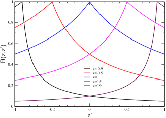
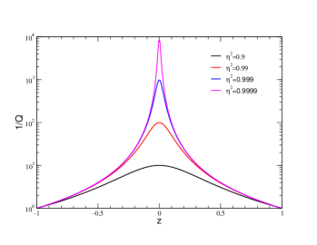
Figure 2: Left panel kernel R(z,z’) defined in (23) and right panel kernel $Q$ defined in (12) for different values of $\eta$.

For $n=1$ there is a single equation determining the unique component of $\Phi_{1}$

$$g_{1}(z)={\lambda\over 2}\;\int_{-1}^{+1}dz^{\prime}\;{R(z,z^{\prime})\over Q(z^{\prime})}\;g_{1}(z^{\prime})$$ (25)

For $n=2$, the solution $\Phi_{2}$ is determined by two components, $g_{2}^{0}$ and $g_{2}^{1}$ , satisfying

$$g_{2}^{0}(z) = {\lambda\over 2}\;\;\;{1\over 2}\int_{-1}^{+1}dz^{\prime}\;{R^{2}(z,z^{\prime})\over Q(z^{\prime})}\;g_{2}^{0}(z^{\prime})$$

$$g_{2}^{1}(z) = {\lambda\over 2}\left[{1\over 3}\;\int_{-1}^{+1}dz^{\prime}\;{R(z,z^{\prime})\over Q^{2}(z^{\prime})}\;g_{2}^{0}(z^{\prime})+\int_{-1}^{+1}dz^{\prime}\;{R(z,z^{\prime})\over Q(z^{\prime})}\;g_{2}^{1}(z^{\prime})\right]$$

For $n=3$ the solution is given by

$$g_{3}^{0}(z) = {\lambda\over 2}\;\;\;{1\over 3}\int_{-1}^{+1}dz^{\prime}\;{R^{3}(z,z^{\prime})\over Q(z^{\prime})}\;g_{3}^{0}(z^{\prime})$$

$$g_{3}^{1}(z) = {\lambda\over 2}\left[c_{3}^{10}\;\int_{-1}^{+1}dz^{\prime}\;{R^{2}(z,z^{\prime})\over Q^{2}(z^{\prime})}\;g_{3}^{0}(z^{\prime})+c_{3}^{11}\int_{-1}^{+1}dz^{\prime}\;{R^{2}(z,z^{\prime})\over Q(z^{\prime})}\;g_{3}^{1}(z^{\prime})\right]$$

$$g_{3}^{2}(z) = {\lambda\over 2}\left[c_{3}^{20}\;\int_{-1}^{+1}dz^{\prime}\;{R(z,z^{\prime})\over Q^{3}(z^{\prime})}\;g_{3}^{0}(z^{\prime})+c_{3}^{21}\int_{-1}^{+1}dz^{\prime}\;{R(z,z^{\prime})\over Q^{2}(z^{\prime})}\;g_{3}^{1}(z^{\prime})+c_{3}^{22}\int_{-1}^{+1}dz^{\prime}\;{R^{2}(z,z^{\prime})\over Q(z^{\prime})}\;g_{3}^{2}(z^{\prime})\right]$$

It is worth noticing that, for each $n$, the component $g_{n}^{0}$ decouples from the rest. It is determined by a single equation

$$g_{n}^{0}(z)={\lambda\over 2n}\;\int_{-1}^{+1}dz^{\prime}\;{R^{n}(z,z^{\prime})\over Q(z^{\prime})}\;g_{n}^{0}(z^{\prime})$$ (26)

and provides the full spectrum of the W-C model. The rest of the components are needed to reconstruct the full BS amplitude and other observables, like, e.g., form factors.

Since (26) is homogeneous, the norm of $g_{n}^{0}$ is not fixed by (26), and can be only determined by normalizing $\Phi_{n}$ in (7). On the contrary, there is no choice in the norm of the components $g_{n}^{\nu>0}$, since they obey an inhomogeneous equation with a source term proportional to $g_{n}^{0}$.

There is an equivalent formulation of (24) in differential form. For instance, eq. (26) providing $g_{n}^{0}$ for any $n$, is equivalent to the differential equation

$${g^{\prime\prime}}_{n}^{0}(z)+{2(n-1)z\over 1-z^{2}}\;{g^{\prime}}_{n}^{0}(z)-{n(n-1)\over 1-z^{2}}\;g_{n}^{0}(z)+{\lambda\over(1-z^{2})Q(z,\eta)}\;g_{n}^{0}(z)=0$$ (27)

with the boundary conditions $g_{n}^{0}(\pm 1)=0$.

For n=2, and after having obtained $g_{2}^{0}$ by (27), the component $g_{2}^{1}$ is a solution of the inhomogeneous equation

$${g^{\prime\prime}}_{2}^{1}+{\alpha\over\pi}{1\over(1-z^{2})Q(z,\eta)}\;g_{2}^{1}=-{\alpha\over 3\pi}\;{1\over(1-z^{2})Q^{2}(z,\eta)}\;g_{2}^{0}$$ (28)

with $g_{2}^{0}$ as a source term, and so forth for the other $n$’s.

3.1 Normal and abnormal states

The W-C model has an infinite family of solutions ($\Phi_{n},M_{n}$), which, for small values of the coupling constant $\alpha$, are ”logarithmically tangent” to the non-relativistic Coulomb bound-state spectrum [8]:

$$B_{n}(\alpha)={m\alpha^{2}\over 4n^{2}}\;\left[1+{4\over\pi}\alpha\ln\alpha+o(\alpha^{2})\right]$$ (29)

where $M_{n}=2m-B_{n}$.

For a given $n$, the function $g_{n}^{0}(z)$ satisfies the homogeneous equation (27), in which $n$ plays role of a parameter. Such equations usually have a whole spectrum of solutions. This just takes place in the equation (27). Therefore, for each value of $n$=1,2,…, there exists an additional series of eigenvalues labeled by a new quantum number $\kappa=0,1,\ldots$, which is a consequence of the symmetry of the 4D Coulomb problem. The components of the corresponding eigenstates $g^{\nu}_{n\kappa}$ have a well defined parity determined by $\kappa$.

$$g_{n\kappa}^{\nu}(-z)=(-)^{\kappa}g^{\nu}_{n\kappa}(z)$$

The subset $\kappa=0$ corresponds, for small values of $\alpha$, to the standard Balmer series (29), that is, to the ”normal” non-relativistic solutions. The other states, with $\kappa\neq 0$ , do not have a counterpart in the non-relativistic theory and for this reason were named by Wick ”abnormal states”. It is worth mentioning that the states with odd values of $\kappa$ have vanishing contributions to the S-matrix [9]. So the first abnormal state with dynamical content is $\kappa=2$.

We have displayed in Fig. 3 the energies of the lower states as a function of the coupling constant $\lambda={\alpha\over\pi}$ in a log-log scale. One sees clearly that two different families of states arise: in solid black lines is the ensemble of normal states ($\kappa=0$) with different values of the principal quantum number $n$. They have an accumulation point in ($\lambda,B$)=(0,0). We have included in black dashed line the non-relativistic limit for the ground state. Colored lines correspond to the ground state ($n=1$) of the abnormal solutions: $\kappa=1$ in red, $\kappa=2$ in green,…. This family is totally decoupled, in its $\lambda(B)$ trajectory, from the first one, though the normal and abnormal series intersect. As seen in Fig. 3, between two excited normal states there are the abnormal ones. The abnormal series has an accumulation point at ($\lambda,B$)=(1/4,0). One can show [5, 6] that, for small values of B, the energies of the abnormal states behave as

$$\lambda(B)\approx{1\over 4}+\frac{4\pi^{2}(\kappa-1)^{2}}{\ln^{2}{B\over m}}$$ (30)

independently of the main quantum number $n$. Notice from Fig. 3 that the asymptotic value $\lambda_{min}=1/4$, independent of $\kappa$, is reached very slowly when $B$ tends to zero. For instance, for $\kappa$=2 and B=10^-6, the value of $\lambda$ is still a factor two larger than $1/4$.

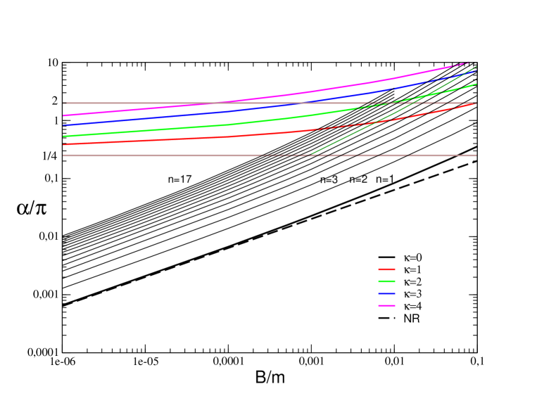
Figure 3: Solid black lines correspond to binding energies of the first (n=1,2,…) normal states ($\kappa=0$) as a function of the coupling constant $\alpha$. Abnormals states, limited to ground n=1, are in colored lines: $\kappa=1$ in red, $\kappa=2$ in green,… .

The fact that this horizontal asymptote is reached always from above means that the abnormal solutions exist only for large values of the coupling constant: $\lambda\geq{1\over 4}$ or $\alpha\geq{\pi\over 4}$. This is the meaning of the horizontal bold brown line at $\lambda=\lambda_{min}=1/4$.

The existence of a minimal coupling constant to bind a two-body system is typical of a Yukawa-like massive-exchange potential. From this point of view, the ground abnormal state ($\kappa=2$) behaves as if it was created by the exchange of a ”massive photon” with a non zero effective mass $\mu_{eff}$. One can get an evaluation of its value by means of the solution of the non-relativistic Yukawa model [31]. One can see there that the minimal coupling constant for the appearance of the first bound state in the dimensionless problem is $G_{0}\approx 1.680$. It is related to the minimal coupling constant of the dimensionful problem by $\alpha_{min}={\mu\over m}G_{0}$. For all abnormal solutions one has $\alpha_{min}=\pi/4$, which gives $\mu_{eff}/m=0.47$.

On another hand, it turns out that for values of $\lambda>2$ the ground state of the model, i.e., the normal state with $n$=1 and $\kappa$=0, has $M^{2}<0$. If we want to restrict ourselves to non-tachyonic states, the coupling constant must be limited to $\lambda\leq\lambda_{max}=2$. This is the reason for the horizontal brown line at $\lambda=\lambda_{max}$ in Fig. 3. Since the first abnormal state is $\kappa$=2 and it crosses the line $\lambda=\lambda_{max}$ at $B\approx 0.00903$, this means that all abnormal states, although requiring large values of the coupling constants to exist, concern very low-energy solutions.

It is quite a paradoxical situation for a relativistic theory to predict a series of new low-energy states. We would like to mention here that the existence of such states, would they be obtained with a simplified kernel, require the full covariance of the theory. If the excitation in the time-like degrees of freedom are frozen, the abnormal states disappear [10].

3.2 Characterization of the abnormal states

In a series of papers [11, 12, 13], summarized in [14], we have studied the properties of the abnormal states in the W-C model, with the main aim of giving an intrinsic characterization of such states, rather than a relative position in the full spectrum of the model.

We have extensively compared the elastic and inelastic form factors of normal versus abnormal states. The most striking difference lies in the two-body contents of the corresponding state vectors. Indeed, in the Light-Front approach, the state vector $\mid P\rangle$ appearing in the definition of the BS amplitude (1) is a QFT state involving many-body components (Fock expansion):

$$\mid P\rangle=\sum_{n\geq 2}^{\infty}\Psi_{n}(k_{1},k_{2},\ldots,k_{,})\mid n\rangle\qquad\mid n\rangle=a^{\dagger}_{k_{1}}a^{\dagger}_{k_{2}},\ldots,a^{\dagger}_{k_{n-2}}b^{\dagger}_{q_{1}}b^{\dagger}_{q_{2}}$$

where the operators $b^{\dagger}$ and $a^{\dagger}$ are the creation operators of the constituent massive particles and of the exchanged particle, respectively, and where $\Psi_{n}$ is, by definition, the n-body wave function.

The total norm of a state vector results from adding the partial norms of the corresponding 2-, 3- and many-body components

$$\langle P\mid P\rangle=1=\int\Psi_{2}^{2}+\int\Psi_{3}^{2}+\int\Psi_{4}^{2}+\ldots=N_{2}+N_{3}+N_{4}+\ldots$$

Having normalized the BS amplitude $\Phi$ by the condition $F$(0)=1, where $F(Q)$ is the elastic electric form factor of the full bound system, we have obtained the two-body wave function by projecting on the Light-Front plane, $\omega\cdot x$=0 with $\omega^{2}=0$, the BS amplitude

$$\psi_{2}(k_{1},k_{2},P,\omega)=\frac{(\omega\cdot k_{1})(\omega\cdot k_{2})}{\pi(\omega\cdot P)}\int_{-\infty}^{+\infty}\Phi(k+\beta\omega,P)\;d\beta$$

and by that, the two-body norm

$$N_{2}=\frac{1}{(2\pi)^{3}}\int\psi_{2}^{2}(k_{\perp},x)\frac{d^{2}k_{\perp}dx}{2x(1-x)}.$$

We have displayed in Fig. 4 the two-body norm $N_{2}$ of the first two normal (left panel) and abnormal (right panel) states as functions of their binding energy $B$. As one can see, an essential difference appears between the two-body contents of a normal and an abnormal state. In the limit of small binding energies, the two-body norm $N_{2}$ of a normal state tends to 1 (left panel) , indicating that it is described by a 2-body. valence wave function. On the contrary, the abnormal states has a two-body norm that, in this $B\to 0$ limit, tends to 0, indicating a genuine many body character of such states. This difference holds for the ground as well as for the first excited states.

This is an intrinsic difference between such kind of states, related to only their very internal structure and independent of their energy, and was probably the most striking result of our previous work [14].

It is worth mentioning here some kind of skepticism expressed by Wick himself, when commenting on the existence of such states at the very end of his seminal article [5]. He wrote ”About the possible existence of these abnormal solutions, we shall not try to speculate. Since they occur only for finite values of $\lambda$ ($\lambda\geq 1/4$) it will be unwise to assume that they are a property of the complete BS equation. Certainly the ladder approximation cannot be trusted to such extent”. To our knowledge, this judicious remark still remains an open question. However the many-body character of the abnormal states that we have put in evidence, seems to provide an argument in favour of their existence. It is hard to imagine a possible mechanism with which the non-ladder many-body contributions could inhibit the construction of such collective many-body states.

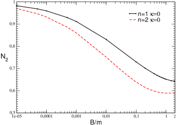
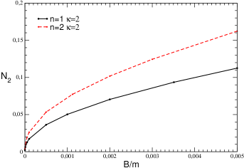
Figure 4: $N_{2}$-dependence on the binding energy $B/m$ for the ground ($n=1$) and first excited ($n=2$) states. On left panel for the normal states ($\kappa=0$) and on right panel for the abnormal ones ($\kappa=2$).

So far we have considered the case of equal constituent masses. If the Coulomb field would be provided by a heavy ion, interacting with an electron, we would deal with strongly unequal constituent masses. The existence of abnormal states in this case was studied in [6, 15]. It turns out that in a system with such different masses the abnormal states still exist. Moreover, the effect of unequal masses is attractive. The balance between the exchanged photons and the massive constituents is little sensitive to the mass ratio, and so the many-photon component still predominates.

It remains to see whether the abnormal states survive when the exchange mass differs from zero. This will be the content of our forthcoming publication [29] . The first results are summarized in the next section.

4 Solutions for the massive-exchange case

The solution of the massive-exchange case can be obtained by directly solving the BS equation in Euclidean space (4). There are however other alternatives which are inspired by the Cutkosky solution of the massless-exchange case, previously discussed. They are also based on a, now two-dimensional, integral representation of the BS amplitude that is due to Nakanishi [16] and that reads

$$\Phi(k,p) = -i\int_{-1}^{1}dz^{\prime}\int_{0}^{\infty}d\gamma\frac{g(\gamma,z)}{\left[\gamma+m^{2}-\frac{1}{4}M^{2}-k^{2}-p\cdot k\;z-i\epsilon\right]^{3}}.$$ (31)

Once inserted in the BS equation, one can obtain an integral equation for the bi-dimensional spectral function $g(\gamma,z)$. This approach was first suggested by Kusaka and Williams [17, 18] with the aim of obtaining the BS solutions in Minkowski space, and has taken different forms during the almost thirty years of sustained developments [19, 20, 21, 22, 23, 24, 25, 26, 27].

Our last formulation [26] is based on a combined use of the Nakanishi representation, the Light-Front projection of the BS amplitude and the Stieltjes transform. The (bound state) BS equation for the weight function $g$ takes the standard form

$$g(\gamma,z)=\int_{0}^{\infty}d\gamma^{\prime}\int_{-1}^{1}dz^{\prime}\;N(\gamma,z;\gamma^{\prime},z^{\prime})\;g(\gamma^{\prime},z^{\prime})$$ (32)

Several, a priori equivalent, forms of the kernel $N$ corresponding to the W-C model can be found in [22, 26, 28].

Although the spectral function $g(\gamma,z)$ is smooth, the kernel $N$ has several moving singularities in both integration variables $\gamma^{\prime},z^{\prime}$. They are of course integrable but must be treated with some care to avoid spurious structures. The detailed analysis of these singularities depends on the particular form of the kernel and will be given in [29].

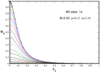
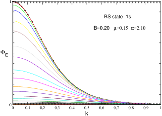
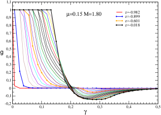
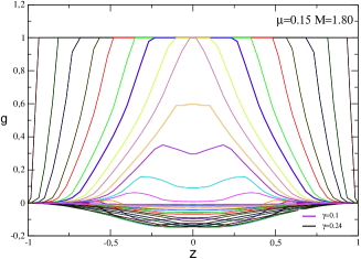
Figure 5: Upper panel: The Euclidean BS amplitude for $\mu=0.15$ and $B=0.2$. On the left, as a function of $k_{4}$ for selected values of $k$, and on the right, as a function of $k$ for selected values of $k_{4}$. Lower panel: the same state in terms of the Nakanishi weight function $g(\gamma,z)$

We display in Fig. 5 two representation of the same state, one (upper part) obtained with the BS solution in Euclidean space (4) and the other one (lower part) with the solution of eq. (32). They correspond to $\mu=0.15$, a binding energy $B=0.2$, with the coupling constant $\alpha=2.10$. If the Euclidean solution in the upper part of the figure is a very smooth function of both arguments, the $\gamma$-dependence of the Nakanishi weight function $g$ is non-trivial. We can show analytically [29] that $g$ is constant in a triangular domain $\Delta$ of the ($\gamma,z$) plane, illustrated in Fig. 6, presents a cusp on its border and evolves continuously outside. The analytic expression of this domain is $\Delta=\{(\gamma,z)\in R^{2}:z\in[-1,+1]\;{\rm and}\;\gamma=\gamma_{0}(z)\}$ with $\gamma_{0}(z)$ given by

$$\gamma_{0}(z)=(1-|z|){M^{2}\over 4m^{2}}\;\left({\mu^{2}\over m^{2}}+4{\mu\over M}\sqrt{1-{M^{2}\over 4m^{2}}}\sqrt{1-{\mu^{2}\over 4m^{2}}}\right)$$ (33)

This peculiar behaviour was missed in our first publications [19, 20] because of some numerical instabilities in the left-hand side kernel and was only vaguely suggested in [22] due to an unadapted basis set used in the numerical solution. It was however well reproduced in Figs. 2 and 3 of [17]. It seems to be also well reproduced in Fig. 5 of Ref. [27], although in this work the domain of constant $g$ is half a circle rather than a triangle, maybe due to the used logarithmic scale or to some change of variable. Notice also that the negative part of $g$, visible in Fig. 5 for $\gamma\sim 0.2$, is totally absent in reference [17] and not clearly seen in [27]. On the contrary the results from [18] are not understandable in terms of the previous analysis.

Figure 6: Domain $\Delta$ of the ($\gamma,z$) where the solution $g(\gamma,z)$ is constant.

When $\mu\neq 0$ the symmetry of the 4D Coulomb problem is lost, as well as the $\kappa$ quantum number identifying the abnormal states in the $\mu$=0 case. The solutions of the BS equation are then labeled by a single quantum number $n$ which tells us nothing about the normal or abnormal character of the state. On another hand, the level ordering of the abnormal states in the $\mu$=0 case depends critically on the binding energy $B$ of the state. As one can see in Fig. 3, for B=0.1, the first abnormal state ($\kappa$=2, $n$=1) (in green) is the 6th excitation in the $\alpha$ spectrum, while for B=0.01 it corresponds to the 11th… and for B=0 there is an infinity of normal states below the first abnormal one. So, even for $\mu$=0, just by computing the $\alpha$ spectrum for a given $B$, there is no way to identify the abnormal state without study its wave function: there is an infinity of level crossing among normal and abnormal states when $B$ is changed.

In a recent work we have extensively studied the survival of the abnormal states in the massive case. The method and the results will be detailed in a forthcoming publication [29]. We present in what follows a summary of the main results concerning the very existence of such states.

The procedure is based on tracing the trajectories of a well-identified abnormal state for $\mu$=0 as a function of $\mu$, and on determining in this way the ensemble of parameters ($\alpha,\mu$) allowing the existence of the abnormal states, as well as their binding energies $B(\alpha,\mu)$. We will restrict here to the non-tachyonic domain of the coupling constant: $1/4<\lambda={\alpha\over\pi}<2$.

An illustrative example is given in the left panel of Fig. 7 for the ground abnormal state ($n$=1, $\kappa$=2) with binding energy $B$=0.007. This state (in blue solid line) corresponds to the 12th excitation at $\mu$=0. When $\mu$ is increased, the corresponding value of $\alpha$ increases until it reaches the maximum allowed value of the coupling constant $\alpha/\pi=2$. This determines, the maximum allowed exchanged mass $\mu$ for this state: $\mu_{max}\approx$0.0030. This result constitutes the first evidence, a numerical proof of existence, of abnormal states in the W-C model with non-zero $\mu$. Such a possibility was considered in Ref. [30], in relation with its eventual contribution to the S-matrix.

By repeating this study for several values of $B$, one can determine $\mu_{max}(B)$, that is the maximum value of $\mu$ compatible with a non-tachyonic ground state solution ($M^{2}>0$) as a function of its binding energy $B$. It is worth noticing here that for $\mu>0$ the non-tachyonic condition is not exactly given by $\alpha=2\pi$ but by a a slightly larger value $\alpha_{max}(\mu)>2\pi$ due to the short-range character of the $\mu>0$ interaction. Since the involved values of $\mu$ are very small, one can take for practical purposes $\alpha_{max}(\mu)=2\pi$. The $\mu_{max}(B)$ dependence is the essential ingredient in our study and it is displayed in the right panel of Fig. 7. The maximum allowed value of the exchanged mass is reached for $B=0$ and is $\mu_{max}(0)=0.087$ (in constituent units).

Figure 7: Left panel: dependence of the $\alpha$-spectrum as a function of $\mu$, for B=0.007. The horizontal dashed line corresponds $\alpha_{max}(\mu)\approx 2\pi$. The trajectory $\alpha(\mu)$ – corresponding to the ground abnormal state (in blue solid line) – remains smaller than $\alpha_{max}(\mu)$ until $\mu\approx$0.0030. The ground abnormal state, which at $\mu$=0 is the 12th excitation of $\alpha$ spectrum, displays a level crossing at $\mu\approx$0.0034 and becomes the 11th excited state. Right panel: by repeating the study for several values of B one determines the domain $\mu_{max}(B)$.

We have repeated this study for several values of the binding energy and obtained the results of Fig. 8. Our technology does not allow us to go below B=10^-5, essentially due to the difficulty of accurately computing higher excited states. For $B$=10^-6 and $B$=0 we have just inserted the values for $\mu$=0. On the other hand, it is worth noticing that the $\mu=0$ limit of the W-C model is non-analytic and highly singular. This is manifested already by the fact that the two-dimensional weigh function $g(\gamma,z)$ generates in this limit a $\delta(\gamma)$ function and there remains only the $z$-dependence. When computing the solutions for very small values of $\mu$ we are faced to this embarrassing vicinity. Let us also mention that the slope at $\mu=0$ of the $\alpha(\mu,B)$ represented at B=0 is infinite.

Figure 8: The parameter window ($\alpha,\mu$) of the ground abnormal state, for several values of B. For $B<10^{-5}$ the ground abnormal state is too high in the excitation spectrum to be numerically accessible: we give only the values of the coupling constant corresponding to $\mu=0$.

The curves displayed in Fig. 8 delineate the parameter domain of the W-C model, for which the abnormal states exist. It constitutes the main result of our work. They allow us to draw two conclusions. The first one is that abnormal states exist for $\mu>0$. The second one is that, due to stability reasons of the theory, their binding energy is smaller than $B/m\approx 0.00903$ and the exchanged mass is limited to very small values of $\mu$, $\mu/m<0.0087$.

5 Conclusion

We have reviewed the main properties of the “abnormal solutions” of the Bethe–Salpeter equation with the Wick–Cutkosky model, i.e., scalar particles with mass $m$ interacting via massless ($\mu$=0) exchange, as wells as its extension to the massive-exchange case.

These are low-energy ($B/m<0.009$) solutions that exist in this particular relativistic approach, but are absent in the non-relativistic limit (Coulomb problem). Their position in the full spectrum of the model is totally decoupled from the normal solutions, which tend to the standard Coulomb states, and require, even in the zero binding limit, a minimal value of the coupling constant, $\alpha_{min}=\pi/4$, to exist. From this point of view the abnormal solutions behave as if they were created by an effective ”massive photon”. In the $\mu=0$ case, this is equivalent to a ”massive photon” with an effective mass of $\mu_{eff}/m\approx 0.47$. For the $\mu>0$ case, the value of $\mu_{eff}$ is roughly the same than for the massless case since the values of $\alpha_{min}$ are practically unchanged with $\mu$ (See left panel of Fig 7).

Discovered by Cutkosky [6] soon after the formulation of the Bethe–Salpeter equation and its first solution in Euclidean space by Wick [5], we have given them [14] an intrinsic characterization in terms of the small two-body norm of their valence wave function, which vanishes in the $B\to 0$ limit. This confers to them a genuine many body status.

We have presented new results concerning the massive-exchange case, where we have obtained the ensemble of parameters of the model, in particular the values of the exchanged mass $\mu$, that allow the existence of such peculiar solutions without spoiling the model by tachyonic states ($M^{2}<0$).

As our previous analysis shows, the reason for the existence of abnormal states, dominated by multi-photon exchange, is the strong electrical field between constituents and therefore it can be hardly affected by the eventual spin degrees of freedom which were not included in our consideration. The experimental creation and observation of these systems do not seem to be an easy task, but they would be of great interest.

Acknowledgments J.C. thanks the financial support from FAPESP (Fundação de Amparo à Pesquisa do Estado de São Paulo) grant 2022/10580-3. H.S. acknowledges financial support from the EU research and innovation programme Horizon 2020, under Grant agreement No. 824093.

References

- [1] J. Carbonell, B. Desplanques, V.A. Karmanov, J.-F. Mathiot, Explicitly covariant light front dynamics and relativistic few-body systems, Phys. Rep. 300, 215 (1998)
- [2] H.A. Bethe, E.E. Salpeter, A relativistic equation for Bound State Problems, Phys. Rev. 82, 309 (1951)
- [3] E.E. Salpeter, H. Bethe, A Relativistic equation for bound-state problems, Phys. Rev. 84, 1232 (1951).
- [4] M. Mangin-Brinet, J. Carbonell, Solutions of the Wick-Cutkosky model in the Light Front Dynamics, Phys. Lett. B 474, 237(2000)
- [5] G.C. Wick, Properties of Bethe-Salpeter wave functions, Phys. Rev. 96, 1124 (1954).
- [6] R.E. Cutkosky, Solutions of a Bethe-Salpeter equation, Phys. Rev. 96, 1135 (1954).
- [7] M. Gell-Mann, F. Low, Bound states in quantum field theory, Phys. Rev. 84 (1951) 350
- [8] G. Feldman, T. Fulton, J. Townsend, Wick equation, the infinite-momentum frame, and perturbation theory, Phys. Rev. D 7, 1814 (1973).
- [9] M. Ciafaloni, P. Menotti, Operator analysis of the Bethe-Salpeter equation, Phys. Rev. 140, B929 (1965).
- [10] H. Jallouli, H. Sazdjian, There are no abnormal solutions of the Bethe-Salpeter equation in the static model. J. Phys. G 22, 1119 (1996).
- [11] V. A. Karmanov, J. Carbonell, H. Sazdjian, Structure and EM form factors of purely relativistic systems, PoS(LC2019)050; arXiv:2001.00401.
- [12] V. A. Karmanov, J. Carbonell, H. Sazdjian, Bound states of purely relativistic nature, EPJ Web Conf. 204 (2019) 01014
- [13] V. A. Karmanov, J. Carbonell, H. Sazdjian, Bound states of relativistic nature, Contribution to NTSE 2018, 1903.02892 [hep-ph]
- [14] J. Carbonell, V.A. Karmanov, H. Sazdjian, Hybrid nature of the abnormal solutions of the Bethe-Salpeter equation in the Wick-Cutkosky model, Eur. Phys. J. C (2021) 81:50
- [15] V.A. Karmanov, Abnormal states with unequal constituent masses, Eur. Phys. J. C (2024) 84:58
- [16] N. Nakanishi, Partial-wave Bethe–Salpeter equation, Phys. Rev. 130, 1230 (1963);General Survey of the Theory of the Bethe-Salpeter Equation, Prog. Theor. Phys. Suppl. 43, 1 (1969); Graph Theory and Feynman Integrals (Gordon and Breach, New York, 1971).
- [17] K. Kusaka and A.G. Williams, Solving the Bethe-Salpeter equation for scalar theories in Minkowski space, Phys. Rev. D 51 (1995) 7026;
- [18] K. Kusaka, K. Simpson and A.G. Williams, Solving the Bethe-Salpeter equation for bound states of scalar theories in Minkowski space, Phys. Rev. D 56 (1997) 5071.
- [19] V.A. Karmanov and J. Carbonell, Solving Bethe-Salpeter equation in Minkowski space, Eur. Phys. J. A 27 (2006) 1.
- [20] J. Carbonell, V.A. Karmanov, Cross-ladder effects in Bethe-Salpeter and light-front equations, Eur. Phys. J. A 27 (2006) 11.
- [21] T. Frederico, G. Salmè and M. Viviani, Two-body scattering states in Minkowski space and the Nakanishi integral representation onto the null plane, Phy. Rev. D 85 036009 (2012)
- [22] T. Frederico, G. Salmè and M. Viviani, Quantitative studies of the homogeneous Bethe-Salpeter equation in Minkowski space, Phy. Rev. D 89 (2014) 016010.
- [23] T. Frederico, G. Salmè and M. Viviani, Solving the inhomogeneous Bethe-Salpeter Equation in Minkowski space: the zero-energy limit, Eur. Phys. J. C 75 (2015) 398.
- [24] W. de Paula, T. Frederico, G. Salmè, M. Viviani, Advances in solving the two-fermion homogeneous Bethe-Salpeter equation in Minkowski space, Phys.Rev. D 94 (2016) 071901.
- [25] C. Gutierrez, V. Gigante, T. Frederico, G. Salmè, M. Viviani, L. Tomio, Bethe?Salpeter bound-state structure in Minkowski space, Phys. Lett. B 759 (2016) 131.
- [26] J. Carbonell, T. Frederico, V.A. Karmanov, Bound state equation for the Nakanishi weight function, Phys. Lett. B, 769, 418 (2017); arXiv:1704.04160.
- [27] Shaoyang Jia, Direct solution of Minkowski-space Bethe-Salpeter equation in the massive Wick-Cutkosky model, Phys. Rev. D 109, 036020 (2024)
- [28] V.A. Karmanov, New form of kernel in equation for Nakanishi function, Phys. Rev. D 104, 056012 (2021)
- [29] J. Carbonell, V.A. Karmanov, E.A. Kupriyanova and H. Sazdjian, Abnormal solutions of the Bethe-Salpeter equation: the massive exchange case, to be published
- [30] S. Naito, S-Matrix and Abnormal Solutions of the Bethe-Salpeter Equation, Prog. Theor. Phys. 40, 628 (1968)
- [31] J. Carbonell · F. de Soto · V. A. Karmanov, Three Different Approaches to the Same Interaction: The Yukawa Model in Nuclear Physics, Few-Body Syst (2013) 54:2255-2269