Stability Certificates for Receding Horizon Games

Sophie Hall, Dominic Liao-McPherson, Giuseppe Belgioioso, Florian Dörfler Sophie Hall, Giuseppe Belgioioso, and Florian Dörfler are with the Automatic Control Laboratory, ETH Zürich, Switzerland. (emails: {shall, gbelgioioso, dorfler}@ethz.ch. Dominic Liao-McPherson is with the University of British Columbia, Vancouver, Canada, (e-mail: dliaomcp@mech.ubc.ca). This work is supported by the SNSF via NCCR Automation (Grant Number 180545).
Abstract

Game-theoretic MPC (or Receding Horizon Games) is an emerging control methodology for multi-agent systems that generates control actions by solving a dynamic game with coupling constraints in a receding-horizon fashion. This control paradigm has recently received an increasing attention in various application fields, including robotics, autonomous driving, traffic networks, and energy grids, due to its ability to model the competitive nature of self-interested agents with shared resources while incorporating future predictions, dynamic models, and constraints into the decision-making process. In this work, we present the first formal stability analysis based on dissipativity and monotone operator theory that is valid also for non-potential games. Specifically, we derive LMI-based certificates that ensure asymptotic stability and are numerically verifiable. Moreover, we show that, if the agents have decoupled dynamics, the numerical verification can be performed in a scalable manner. Finally, we present tuning guidelines for the agents’ cost function weights to fulfil the certificates and, thus, ensure stability.

Index Terms:
game theory, model predictive control (MPC), dissipativity, input-to-state stability

I Introduction

Our modern society is underpinned by a multitude of shared infrastructure and resources (e.g., traffic networks, power grids, and fish stocks). These systems and resources need to be carefully managed; if left unchecked, selfish behavior by users can lead to severe societal losses: selfish routing decisions lead to traffic congestion [1], selfish energy consumption causes blackouts [2], and overfishing leads to the collapse of fish stocks [3]. The need to make these critical systems more resilient is driving the development of resource allocation protocols that manage them in a fair and sustainable way.

In many cases these decisions need to be made in real-time through control algorithms. Controlling shared infrastructure and allocating resources in real-time is a challenging problem for multiple reasons: (i) it requires optimization of general economic cost functions, (ii) resource availability and prices are time-varying requiring predictions into the future (e.g., fish stock varies with the seasons and electricity prices vary with renewable generation), (iii) enforcing local and global constraints is necessary as system infrastructure underlies strict operating conditions and shared resources are limited, (iv) large-scale systems require efficient distributed solution algorithms. One of the only systematic and tractable control frameworks for systems with these properties is Economic Model Predictive Control (EMPC) as it allows for general economic objectives and constraints as well as for distributed implementations [4]. However, EMPC implicitly assumes that agents accessing the shared resources are willing to cooperate fully to achieve a socially-optimal outcome. Making such an assumption seems unreasonable, it is well established that self-interested agents accessing a shared resource optimize for their own benefit, e.g., see the infamous tragedy of the commons [5], leading to outcomes that are far from socially optimal [6].

Game-theory comes to the rescue as a powerful tool for modeling conflict and cooperation between self-interested decision makers. In particular, network games have been used extensively to study resource allocation problems, see [7] and references therein. However, these works assume the system is in steady-state whereas in reality most engineering and natural systems are governed by dynamics. Neglecting these means that (i) transients are not optimized [8], (ii) constraints may be violated, and (iii) solutions may not coincide with steady states of the system [9]. Moreover, introducing feedback into the system is essential for robustness against disturbances and model mismatch. One approach to do so is to use explicit game-theoretic feedback policies [10], however for the setting with coupling constraints these policies are expensive to compute and only approximate schemes exist to date [11]. Another approach is to solve the game in a receding-horizon fashion, measuring the state and recomputing the open-loop trajectory at every sampling time, à la MPC.

The combination of MPC and game theory, also called Receding Horizon Games (RHG) [12] or Game-Theoretic Planning [13, 14], allows to handle systems with dynamics, constraints, and self-interested agents. This control paradigm have been already successfully employed in various engineering applications, including supply chains [15], robotics [16], autonomous driving [17, 14, 18], electric vehicle charging [19], and smart grids [20, 12]. Despite its widespread application, RHG still lacks the rigorous underpinning of MPC, such as stability and recursive feasibility. Yet, for large-scale infrastructures such theoretical guarantees are essential to ensure efficient, safe, and reliable operation at all times.

Up to now such guarantees have only been established for strongly monotone potential games played in receding-horizon [12, 21]. Note that for dynamic resource allocation problems potential games are idealized and practically very restrictive as they constrain agent’s cost function design and thus cannot model scenarios where agents truly act in their own self-interest. The authors in [21] discuss a receding-horizon implementation of a game-theoretic traffic routing system and show stability under a strong monotonicity assumption for a potential cost which is proven to be a control Lyapunov function of the closed-loop system. In [22] a game-theoretic distributed MPC with coupled dynamics and local input constraints is designed. A potential-like global cost function is derived through weighted sums of strongly convex stage costs and closed-loop stability is proven.
Refer to caption
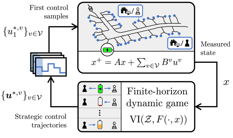
Figure 1: In RHG, control actions are generated by solving a finite-horizon dynamic game, in a receding-horizon fashion.

In this paper, we leverage monotone operator theory and dissipativity theory to develop the first general stability analysis of RHG. Overall, the paper makes the following three main contributions:

  1. 1.

    We derive a sufficient condition for the closed-loop stability of RHG controllers that can be numerically verified by solving a linear matrix inequality (LMI). Our certificates cover RHG controllers with strongly monotone games and linear stable dynamics. Moreover, we establish conditions under which these certificates can be computed in a distributed manner.

  2. 2.

    We derive analytical solutions to the LMIs in a simplified setting and identify key factors affecting the closed-loop stability of RHG controllers. Based on these analytical results, we provide local tuning recommendations for RHG guidelines.

  3. 3.

    We validate the effectiveness of our stability certificates and tuning guidelines via a case study on a battery charging scenario, demonstrating their practical applicability in real-world settings.

Our stability analysis is related to the technical analysis in [23], where linear state feedback matrices K𝐾K are designed to guide a group of self-interested agents to a co-evolutionary equilibrium. Stability certificates for strongly monotone games are derived by leveraging similar dissipativity tools. However, the focus lies on the design of incentives without predictions, which differs significantly from the perspective of our work.

II Preliminaries

II-1 Basic notation

We denote by K={0,,K1}subscript𝐾0𝐾1\mathbb{Z}_{K}=\{0,\dots,K\!-\!1\} the sequence of the first K𝐾K non-negative integers. The set of positive definite symmetric matrices of dimension n×n𝑛𝑛n\times n is denoted as 𝕊0nsuperscriptsubscript𝕊succeedsabsent0𝑛\mathbb{S}_{\succ 0}^{n}. Given M𝑀M vectors u1,,uMsuperscript𝑢1superscript𝑢𝑀u^{1},...,u^{M}, we denote by u=col(uv)v=0M:=[(u1),,(uM)]𝑢colsuperscriptsubscriptsuperscript𝑢𝑣𝑣0𝑀assignsuperscriptsuperscriptsuperscript𝑢1topsuperscriptsuperscript𝑢𝑀toptopu=\text{col}(u^{v})_{v=0}^{M}:=[(u^{1})^{\top},\ldots,(u^{M})^{\top}]^{\top} the stacked vector of vectors uvsuperscript𝑢𝑣u^{v}. Given K𝐾K matrices, blkdiag(Hi)i=0Kblkdiagsuperscriptsubscriptsubscript𝐻𝑖𝑖0𝐾\text{blkdiag}(H_{i})_{i=0}^{K} denotes the block diagonal matrix with H1,,HKsubscript𝐻1subscript𝐻𝐾H_{1},...,H_{K} on the main diagonal. The spectral radius of H𝐻H is ρ(H)𝜌𝐻\rho(H).

II-2 Operator Theory

A set-valued operator T:qq:𝑇superscript𝑞superscript𝑞T:\mathbb{R}^{q}\rightrightarrows\mathbb{R}^{q} is (μlimit-from𝜇\mu-strongly) monotone if xy,uv0,𝑥𝑦𝑢𝑣0\langle x-y,u-v\rangle\geq 0, (μxy2absent𝜇superscriptnorm𝑥𝑦2\geq\mu\leavevmode\nobreak\ \|x-y\|^{2}), x,yqfor-all𝑥𝑦superscript𝑞\forall x,y\in\mathbb{R}^{q}, with uT(x),vT(y)formulae-sequence𝑢𝑇𝑥𝑣𝑇𝑦u\in T(x),v\in T(y). A single-valued operator S:qq:𝑆superscript𝑞superscript𝑞S:\mathbb{R}^{q}\to\mathbb{R}^{q} is βlimit-from𝛽\beta-cocoercive if xy,S(x)S(y)βS(x)S(y)2𝑥𝑦𝑆𝑥𝑆𝑦𝛽superscriptnorm𝑆𝑥𝑆𝑦2\langle x-y,S(x)-S(y)\rangle\geq\beta\leavevmode\nobreak\ \|S(x)-S(y)\|^{2} for all x,yq𝑥𝑦superscript𝑞x,y\in\mathbb{R}^{q}; S𝑆S is limit-from\ell-Lipschitz if S(x)S(y)xynorm𝑆𝑥𝑆𝑦norm𝑥𝑦\|S(x)-S(y)\|\leq\ell\|x-y\|.

III Receding Horizon Games

Consider a linear time-invariant (LTI) system of the form

xt+1=Axt+v𝒱Bvutv,subscript𝑥𝑡1𝐴subscript𝑥𝑡subscript𝑣𝒱superscript𝐵𝑣subscriptsuperscript𝑢𝑣𝑡\displaystyle x_{t+1}=A\,x_{t}+\sum_{v\in\mathcal{V}}B^{v}\,u^{v}_{t}, (1)

which is controlled by a group of agents v𝒱={1,,M}𝑣𝒱1𝑀v\in\mathcal{V}=\{1,\dots,M\} where xtnxsubscript𝑥𝑡superscriptsubscript𝑛𝑥x_{t}\in\mathbb{R}^{n_{x}} is the global state at time t𝑡t and utvnuvsuperscriptsubscript𝑢𝑡𝑣superscriptsubscriptsuperscript𝑛𝑣𝑢u_{t}^{v}\in\mathbb{R}^{n^{v}_{u}} is the input of agent v𝑣v. At time step t𝑡t (or stage), agent v𝑣v incurs the cost

v(xt,utv,utv)=xtWvxt+(wv)xt+uv(utv,utv),superscript𝑣subscript𝑥𝑡subscriptsuperscript𝑢𝑣𝑡subscriptsuperscript𝑢𝑣𝑡superscriptsubscript𝑥𝑡topsuperscript𝑊𝑣subscript𝑥𝑡superscriptsuperscript𝑤𝑣topsubscript𝑥𝑡superscriptsubscript𝑢𝑣superscriptsubscript𝑢𝑡𝑣superscriptsubscript𝑢𝑡𝑣\displaystyle\ell^{v}(x_{t},u^{v}_{t},u^{-v}_{t})=x_{t}^{\top}W^{v}x_{t}+(w^{v})^{\top}x_{t}+\ell_{u}^{v}(u_{t}^{v},u_{t}^{-v}), (2)

where uv:nu:superscriptsubscript𝑢𝑣superscriptsubscript𝑛𝑢\ell_{u}^{v}:\mathbb{R}^{n_{u}}\to\mathbb{R} is the actuation cost for agent v𝑣v. This so-called stage cost depends on the global state xtsubscript𝑥𝑡x_{t}, the local control input utvsubscriptsuperscript𝑢𝑣𝑡u^{v}_{t}, and the input of all other agents. Additionally, agent v𝑣v must satisfy at all times the following constraints:

utvsubscriptsuperscript𝑢𝑣𝑡\displaystyle u^{v}_{t} 𝒰vabsentsuperscript𝒰𝑣\displaystyle\in\mathcal{U}^{v} (3a)
(utv,utv)superscriptsubscript𝑢𝑡𝑣superscriptsubscript𝑢𝑡𝑣\displaystyle(u_{t}^{v},u_{t}^{-v}) 𝒞,absent𝒞\displaystyle\in\mathcal{C}, (3b)

where (3a) models local input constraints and (3b) is a joint coupling constraint which models the agents access to a shared resource.

Overall, each agent v𝒱𝑣𝒱v\in\mathcal{V} aims to minimize its infinite horizon cost while satisfying both local and coupling constraints, namely,

v𝒱:{minuv,xk=0v(xk,ukv,ukv)s.t.xk+1=Axk+v𝒱Bvukv,kukv𝒰v,k(ukv,ukv)𝒞,kx0=𝐱,:𝑣𝒱casesmissing-subexpressionmissing-subexpressionsubscriptsuperscript𝑢𝑣𝑥superscriptsubscript𝑘0superscript𝑣subscript𝑥𝑘subscriptsuperscript𝑢𝑣𝑘superscriptsubscript𝑢𝑘𝑣missing-subexpressionmissing-subexpressionmissing-subexpressions.t.formulae-sequencesubscript𝑥𝑘1𝐴subscript𝑥𝑘subscript𝑣𝒱superscript𝐵𝑣subscriptsuperscript𝑢𝑣𝑘𝑘subscriptmissing-subexpressionmissing-subexpressionmissing-subexpressionmissing-subexpressionformulae-sequencesuperscriptsubscript𝑢𝑘𝑣superscript𝒰𝑣𝑘subscriptmissing-subexpressionmissing-subexpressionmissing-subexpressionmissing-subexpressionformulae-sequencesuperscriptsubscript𝑢𝑘𝑣subscriptsuperscript𝑢𝑣𝑘𝒞𝑘subscriptmissing-subexpressionmissing-subexpressionmissing-subexpressionmissing-subexpressionsubscript𝑥0𝐱missing-subexpression\displaystyle v\in\mathcal{V}:\left\{\begin{array}[]{r llll}&&\displaystyle\min_{u^{v},\,x}&\;\displaystyle\sum_{k=0}^{\infty}\ell^{v}(x_{k},u^{v}_{k},u_{k}^{-v})\\ &&\textrm{s.t.}&x_{k+1}=A\,x_{k}+{\textstyle\sum_{v\in\mathcal{V}}}B^{v}\,u^{v}_{k},\quad k\in\mathbb{Z}_{\infty}\\ &&&u_{k}^{v}\in\mathcal{U}^{v},\hskip 95.00014ptk\in\mathbb{Z}_{\infty}\\ &&&(u_{k}^{v},u^{-v}_{k})\in\mathcal{C},\hskip 72.00008ptk\in\mathbb{Z}_{\infty}\\ &&&x_{0}=\mathbf{x},\end{array}\right. (9)

where 𝐱𝐱\mathbf{x} is the initial state of systems (1).

However, as (9) is generally computationally intractable, we consider instead the finite-horizon version:

minuv,xsubscriptsuperscript𝑢𝑣𝑥\displaystyle\displaystyle\min_{u^{v},\,x} k=0K1v(xk,ukv,ukv)superscriptsubscript𝑘0𝐾1superscript𝑣subscript𝑥𝑘subscriptsuperscript𝑢𝑣𝑘superscriptsubscript𝑢𝑘𝑣\displaystyle\;\displaystyle\sum_{k=0}^{K-1}\ell^{v}(x_{k},u^{v}_{k},u_{k}^{-v}) (10a)
s.t. xk+1=Axk+v𝒱Bvukv,kKformulae-sequencesubscript𝑥𝑘1𝐴subscript𝑥𝑘subscript𝑣𝒱superscript𝐵𝑣subscriptsuperscript𝑢𝑣𝑘𝑘subscript𝐾\displaystyle x_{k+1}=A\,x_{k}+{\textstyle\sum_{v\in\mathcal{V}}}B^{v}\,u^{v}_{k},\quad k\in\mathbb{Z}_{K} (10b)
ukv𝒰v,kKformulae-sequencesuperscriptsubscript𝑢𝑘𝑣superscript𝒰𝑣𝑘subscript𝐾\displaystyle u_{k}^{v}\in\mathcal{U}^{v},\hskip 95.00014ptk\in\mathbb{Z}_{K} (10c)
(ukv,ukv)𝒞,kKformulae-sequencesuperscriptsubscript𝑢𝑘𝑣subscriptsuperscript𝑢𝑣𝑘𝒞𝑘subscript𝐾\displaystyle(u_{k}^{v},u^{-v}_{k})\in\mathcal{C},\hskip 72.00008ptk\in\mathbb{Z}_{K} (10d)
x0=𝐱,subscript𝑥0𝐱\displaystyle x_{0}=\mathbf{x}, (10e)

where K>1𝐾1K>1 is the prediction horizon. Note that we do not include terminal ingredients in the RHG problem (10) which is commonly done in MPC. These M𝑀M inter-dependent optimal control problems (OCPs), parametric in 𝐱𝐱\mathbf{x}, constitute a non-cooperative generalized game, in which both cost and admissible decision set of each agent depend on others [24]. To synthesize an RHG feedback law based on the coupled OCPS in (10), we first define the global decision set

𝒵=v𝒱𝒰v𝒞.𝒵subscriptproduct𝑣𝒱superscript𝒰𝑣𝒞\displaystyle\mathcal{Z}=\prod_{v\in\mathcal{V}}\mathcal{U}^{v}\leavevmode\nobreak\ \cap\leavevmode\nobreak\ \mathcal{C}. (11)

Then, we substitute the dynamics (10b) and initial condition (10e) of every agent into their stage cost (10a). This results in the following compact formulation of the game (10):

v𝒱:{minuvJv(uv,uv,𝐱)s.t.(uv,uv)𝒵,\forall v\in\mathcal{V}:\quad\left\{\begin{array}[]{rl}\displaystyle\min_{u^{v}}&{J^{v}(u^{v},u^{-v},\mathbf{x})}\\ \textrm{s.t.}&(u^{v},u^{-v})\in\mathcal{Z},\end{array}\right. (12)

where Jv(uv,uv,𝐱)superscript𝐽𝑣superscript𝑢𝑣superscript𝑢𝑣𝐱J^{v}(u^{v},u^{-v},\mathbf{x}) corresponds to (10a) with the dynamics (10b) substituted into it. A set of strategies col(u,v)v𝒱colsubscriptsuperscript𝑢𝑣𝑣𝒱\mathrm{col}(u^{*,v})_{v\in\mathcal{V}} that simultaneously solve (12) is a generalized Nash equilibrium (GNE), see [25] for a formal definition. Among all possible GNEs, we consider the subclass of variational GNEs (v-GNEs), which correspond to the solutions of the following generalized equation:

F(u,𝐱)+𝒩𝒵(u)0,0Fsuperscript𝑢𝐱subscript𝒩𝒵superscript𝑢\displaystyle\text{F}(u^{*},\mathbf{x})+\mathcal{N}_{\mathcal{Z}}(u^{*})\ni 0, (13)

where F(u,𝐱)=col(uvJv(uv,uv,𝐱))v𝒱𝑢𝐱colsubscriptsubscriptsuperscript𝑢𝑣superscript𝐽𝑣superscript𝑢𝑣superscript𝑢𝑣𝐱𝑣𝒱(u,\mathbf{x})=\text{col}(\nabla_{u^{v}}J^{v}(u^{v},u^{-v},\mathbf{x}))_{v\in\mathcal{V}} is the pseudo-gradient of (12), and 𝒩𝒵subscript𝒩𝒵\mathcal{N}_{\mathcal{Z}} is the normal cone [26, Def. 6.38] of the global decision set 𝒵𝒵\mathcal{Z} in (11). We note that 𝒩𝒵subscript𝒩𝒵\mathcal{N}_{\mathcal{Z}} can be given explicitly for all standard constraint sets. Variational GNEs are often desirable solutions for dynamic resource allocation problems as they satisfy coupling constraints (3b), are strategically-(Nash-)stable, i.e., no agent has an incentive to deviate from their agreed upon decision, and are “economically fair”, since each agent incurs the same marginal loss due to the presence of the coupling constraints [25].

We define the mapping from initial state 𝐱𝐱\mathbf{x} to the solutions of the generalized equation (13), or equivalently, to the v-GNEs of (10), as

𝒮(𝐱)={u|F(u,𝐱)+𝒩𝒵(u)0}.𝒮𝐱conditional-set𝑢0𝐹𝑢𝐱subscript𝒩𝒵𝑢\displaystyle\mathcal{S}(\mathbf{x})=\{u\leavevmode\nobreak\ |\leavevmode\nobreak\ F(u,\mathbf{x})+\mathcal{N}_{\mathcal{Z}}(u)\ni 0\}. (14)

In the remainder of this section, we proceed under the assumption that 𝒮𝒮\mathcal{S} is always well-defined and single-valued. Precise conditions ensuring this will be formalized later in Assumption 1.

To approximate a solution of the infinite-horizon game (9), we recursively solve the finite-horizon version (10), in a receding-horizon fashion. Specifically, at each sampling time t𝑡t, the agents compute the v-GNE of the game (10) with measured state 𝐱tsubscript𝐱𝑡\mathbf{x}_{t}, i.e., u=col(uk)kKsuperscript𝑢colsubscriptsuperscriptsubscript𝑢𝑘𝑘subscript𝐾u^{*}=\text{col}(u_{k}^{*})_{k\in\mathbb{Z}_{K}}, and then apply the first element u0subscriptsuperscript𝑢0u^{*}_{0} of the optimal control trajectory. This creates an implicit feedback policy κ𝜅\kappa (referred to as the RHG feedback law) defined as

ut=κ(𝐱t)=Ξ𝒮(𝐱t),subscriptsuperscript𝑢𝑡𝜅subscript𝐱𝑡Ξ𝒮subscript𝐱𝑡\displaystyle u^{*}_{t}=\kappa(\mathbf{x}_{t})=\Xi\,\mathcal{S}(\mathbf{x}_{t}), (15)

where ΞΞ\Xi is a selection matrix that extracts the first element of the control sequence of each agent v𝒱𝑣𝒱v\in\mathcal{V}, namely, u0,vsuperscriptsubscript𝑢0𝑣u_{0}^{*,v}. The resulting closed-loop system under the RHG feedback law (15) is

xt+1=Axt+Bκ(𝐱t),v𝒱formulae-sequencesubscript𝑥𝑡1𝐴subscript𝑥𝑡𝐵𝜅subscript𝐱𝑡for-all𝑣𝒱\displaystyle x_{t+1}=A\,x_{t}+B\,\kappa(\mathbf{x}_{t}),\quad\forall v\in\mathcal{V} (16)

where B=[B1,,BM]𝐵superscript𝐵1superscript𝐵𝑀B=[B^{1},\dots,B^{M}] collects the local Bvsuperscript𝐵𝑣B^{v} matrices in (1).

IV Stability Conditions

In this section, we derive conditions under which the closed-loop system (16) is stable. We make the following standing assumptions.

Assumption 1.

The following conditions hold:

  • (i)

    The open-loop dynamics (1) are stable, i.e., ρ(A)<1𝜌𝐴1\rho(A)<1.

  • (ii)

    The coupling constraint set 𝒞𝒞\mathcal{C} and the local sets 𝒰v,v𝒱superscript𝒰𝑣for-all𝑣𝒱\mathcal{U}^{v},\forall v\in\mathcal{V}, are closed and convex; the set 𝒵𝒵\mathcal{Z} is compact and non-empty; the function uvsuperscriptsubscript𝑢𝑣\ell_{u}^{v} is continuous and uv(,uv)superscriptsubscript𝑢𝑣superscript𝑢𝑣\ell_{u}^{v}(\cdot,u^{-v}) is strongly convex and continuously-differentiable, for any fixed uvsuperscript𝑢𝑣u^{-v}.

  • (iii)

    The pseudo-gradient F(,𝐱)𝐹𝐱F(\cdot,\mathbf{x}) in (13) is μlimit-from𝜇\mu-strongly monotone for any fixed 𝐱𝐱\mathbf{x}.

Assumption 1(i) is widely adopted in studies utilizing dissipativity concepts. Assumption 1(ii) aligns with the standard requirements of regularity and convexity of game-theoretic works  [25]. Coupled with Assumption 1(iii), these conditions ensures existence and uniqueness of a v-GNE [27, Th. 2.3.3], as formalized next. Within the classic MPC framework, the latter assumption corresponds to strong convexity of the stage cost.

Proposition 1.

Under Assumption 1, the solution mapping 𝒮(𝐱)𝒮𝐱\mathcal{S}(\mathbf{x}) in (14) maps to a singleton, for all arguments 𝐱nx𝐱superscriptsubscript𝑛𝑥\mathbf{x}\in\mathbb{R}^{n_{x}}.

Proof.

The normal cone of a convex set 𝒩𝒵subscript𝒩𝒵\mathcal{N}_{\mathcal{Z}} is maximally monotone, and F(,𝐱)𝐹𝐱F(\cdot,\mathbf{x}) is strongly monotone by Assumption 1 (ii). Thus, 𝒮(𝐱)𝒮𝐱\mathcal{S}(\mathbf{x}) in (14) maps to a singleton by  [26, Cor. 23.37]. ∎

The core idea of our analysis is to view the closed-loop system (16) as a feedback interconnection of two dissipative systems, an LTI system and a static nonlinearity. We leverage known links between monotone operator theory and dissipativity to derive conditions which ensure asymptotic stability of this interconnection [28, Def. 2.14].

By exploiting the separable structure of the stage costs in (2), we can write the pseudo-gradient mapping in (17) as

F(u,𝐱)=Fu(u)+Fx𝐱𝐹𝑢𝐱subscript𝐹𝑢𝑢subscript𝐹𝑥𝐱\displaystyle F(u,\mathbf{x})=F_{u}(u)+F_{x}\mathbf{x} (17)

where the expressions for Fu()subscript𝐹𝑢F_{u}(\cdot) and Fxsubscript𝐹𝑥F_{x} are given in (A-A) and  (41), respectively. With this result in place, we can define the mapping

ϕ()=(Fu+𝒩𝒵)1()italic-ϕsuperscriptsubscript𝐹𝑢subscript𝒩𝒵1\displaystyle\phi(\cdot)=(F_{u}+\mathcal{N}_{\mathcal{Z}})^{-1}(\cdot) (18)

which facilitates deriving a more explicit expression for 𝒮𝒮\mathcal{S}. The mapping ϕ()italic-ϕ\phi(\cdot) obeys the following technical properties.

Proposition 2.

The mapping ϕ()italic-ϕ\phi(\cdot) is μlimit-from𝜇\mu-cocoercive and 1μ1𝜇\frac{1}{\mu}-Lipschitz.

Proof.

This results from ϕ()italic-ϕ\phi(\cdot) being the inverse mapping of a μlimit-from𝜇\mu-strongly monotone operator  [26, Ex. 22.7]. ∎

Based on this definition of ϕ()italic-ϕ\phi(\cdot), the mapping 𝒮𝒮\mathcal{S} corresponds to ϕ(Fx)italic-ϕsubscript𝐹𝑥\phi\circ(-F_{x}), and we can rewrite the parametrized equation in (13) as

u=ϕ(Fx𝐱).𝑢italic-ϕsubscript𝐹𝑥𝐱\displaystyle u=\phi(-F_{x}\mathbf{x}). (19)

In turn, we can write closed-loop system (16) as an LTI system

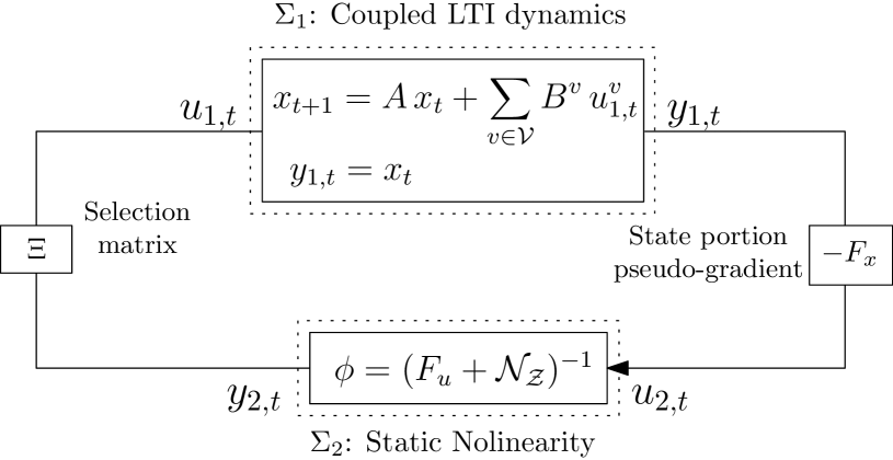
Σ1:{xt+1=Axt+v𝒱Bvu1,tvy1,t=xt,:subscriptΣ1casessubscript𝑥𝑡1absent𝐴subscript𝑥𝑡subscript𝑣𝒱superscript𝐵𝑣subscriptsuperscript𝑢𝑣1𝑡subscript𝑦1𝑡absentsubscript𝑥𝑡\displaystyle\Sigma_{1}:\left\{\begin{array}[]{rl}x_{t+1}&=\displaystyle A\,x_{t}+\sum_{v\in\mathcal{V}}B^{v}\,u^{v}_{1,t}\\ y_{1,t}&=x_{t},\end{array}\right. (22)

in feedback with the static nonlinear map

Σ2:y2,t=ϕ(u2,t),:subscriptΣ2subscript𝑦2𝑡italic-ϕsubscript𝑢2𝑡\displaystyle\Sigma_{2}:y_{2,t}=\phi(u_{2,t}), (23)

and connected through

u1,t=Ξy2,t,u2,t=Fxy1,t,formulae-sequencesubscript𝑢1𝑡Ξsubscript𝑦2𝑡subscript𝑢2𝑡subscript𝐹𝑥subscript𝑦1𝑡\displaystyle u_{1,t}=\Xi\leavevmode\nobreak\ y_{2,t},\quad u_{2,t}=-F_{x}\leavevmode\nobreak\ y_{1,t}, (24)

where (ui,t,yi,t)subscript𝑢𝑖𝑡subscript𝑦𝑖𝑡(u_{i,t},y_{i,t}) are the input and output of system ΣisubscriptΣ𝑖\Sigma_{i} with i{1,2}𝑖12i\in\{1,2\}. The matrix ΞΞ\Xi given in (15) selects the first entry of the optimal predicted input sequence, and Fxsubscript𝐹𝑥F_{x} is the pseudo-gradient of the state cost over the horizon given in (41). The whole interconnection (22)–(24) is shown in Figure 2.
Refer to caption
Figure 2: Feedback interconnection between LTI system Σ1subscriptΣ1\Sigma_{1} and the static nonlinearity ϕ()italic-ϕ\phi(\cdot) in Σ2subscriptΣ2\Sigma_{2}.

Building on this view of RHG in (16) as an interconnection of two dissipative systems, we proceed to establish our main stability result.

Theorem 1.

Suppose that Assumption 1 holds, and that there exists P𝕊0nx𝑃superscriptsubscript𝕊succeedsabsent0subscript𝑛𝑥P\in\mathbb{S}_{\succ 0}^{n_{x}}, λ10subscript𝜆10\lambda_{1}\geq 0 and λ20subscript𝜆20\lambda_{2}\geq 0, with λ1+λ2>0subscript𝜆1subscript𝜆20\lambda_{1}+\lambda_{2}>0, such that

[APAPAPB^B^PB^]+[λ2μ2FxFxλ12Fx(λ1μ+λ2)I]ϵI,precedes-or-equalsmatrixsuperscript𝐴top𝑃𝐴𝑃superscript𝐴top𝑃^𝐵superscript^𝐵top𝑃^𝐵matrixsubscript𝜆2superscript𝜇2superscriptsubscript𝐹𝑥topsubscript𝐹𝑥subscript𝜆12superscriptsubscript𝐹𝑥topsubscript𝜆1𝜇subscript𝜆2𝐼italic-ϵ𝐼\displaystyle\begin{bmatrix}A^{\top}PA-P&A^{\top}P\hat{B}\\ *&\hat{B}^{\top}P\hat{B}\end{bmatrix}+\begin{bmatrix}\frac{\lambda_{2}}{\mu^{2}}F_{x}^{\top}F_{x}&-\frac{\lambda_{1}}{2}F_{x}^{\top}\\ *&-(\lambda_{1}\mu+\lambda_{2})I\end{bmatrix}\preceq-\epsilon I, (25)

for some ϵ>0italic-ϵ0\epsilon>0, where B^=BΞ^𝐵𝐵Ξ\hat{B}=B\,\Xi, μ𝜇\,\mu is the strong monotonicity constant of the operator Fu()subscript𝐹𝑢F_{u}(\cdot) given in (A-A), and Fxsubscript𝐹𝑥F_{x} as in (41). Then, the following conditions hold:

  • (i)

    there exists a globally asymptotically stable equilibrium point, x¯n¯𝑥superscript𝑛\bar{x}\in\mathbb{R}^{n}, of the closed-loop system (16);

  • (ii)

    the OCP in (10) is recursively feasible, 𝐱nxfor-all𝐱superscriptsubscript𝑛𝑥\forall\,\mathbf{x}\in\mathbb{R}^{n_{x}}; and

  • (iii)

    the control inputs satisfy constraints for all times, ut𝒵tsubscript𝑢𝑡𝒵for-all𝑡u_{t}\in\mathcal{Z}\;\forall t.

Proof.

See Appendix A-A. ∎

Theorem 1 provides sufficient conditions for stability based on the monotonicity property of the pseudo-gradient in (17) and dissipativity of the LTI system (1). Dissipativity generalizes both small gain and passivity-based interconnection theorems. This analysis captures how the stable LTI system is affected by the control input generated by solving the non-cooperative game defined in the RHG feedback law in (15). Note that we do not require terminal ingredients to derive the stability certificate in Theorem 1. Moreover, the certificate is easily verified as checking for the existence of P,λ1,𝑃subscript𝜆1P,\lambda_{1}, and λ2subscript𝜆2\lambda_{2} can be posed as a convex program and solved in Python using CVXPY [29].

The LMI in Theorem 1 gives a sufficient but not necessary condition for stability of in (15). The results are conservative due to the analysis strategy which relies on dissipativity of interconnected systems and which treats the feedback term in Σ2subscriptΣ2\Sigma_{2} as perturbation to the coupled LTI dynamics Σ1subscriptΣ1\Sigma_{1}.

Our stability analysis relies on an equilibrium-independent Lyapunov function and, in general, offers no characterization of the equilibrium point itself. However, an expression for x¯¯𝑥\bar{x} can be found if an additional terminal-state constraint is imposed.

Proposition 3.

Let Assumption 1 hold, and denote by (us,xs)subscript𝑢𝑠subscript𝑥𝑠(u_{s},x_{s}), the unique v-GNE of the steady-state game

v𝒱:{minuv,xv(x,uv,uv)s.tx=Ax+Buuv𝒰v,(uv,uv)𝒞,:𝑣𝒱casessubscriptsuperscript𝑢𝑣𝑥superscript𝑣𝑥superscript𝑢𝑣superscript𝑢𝑣s.t𝑥𝐴𝑥𝐵𝑢missing-subexpressionformulae-sequencesuperscript𝑢𝑣superscript𝒰𝑣superscript𝑢𝑣superscript𝑢𝑣𝒞\displaystyle v\in\mathcal{V}:\left\{\begin{array}[]{r l}\displaystyle\min_{u^{v},x}&\;\ell^{v}(x,u^{v},u^{-v})\\ \text{s.t}&x=A\,x+B\,u\\ &u^{v}\in\mathcal{U}^{v},(u^{v},u^{-v})\in\mathcal{C},\\ \end{array}\right. (29)

If usint𝒵subscript𝑢𝑠int𝒵u_{s}\in\text{int}\,\mathcal{Z}, then (us,xs)subscript𝑢𝑠subscript𝑥𝑠(u_{s},x_{s}) is the unique equilibrium point of the closed-loop system (16) for the RHG feedback law defined by the game in (10) with the additional terminal state constraint xK=xssubscript𝑥𝐾subscript𝑥𝑠x_{K}=x_{s}.

Proof.

See Appendix A-B. ∎

RHGs are a generalization of economic MPC (EMPC) to a game-theoretic setting. A RHG collapses into EMPC if there is only one agent, and we can use stability results for EMPC [12] if the game admits a potential. For EMPC without terminal ingredients under dissipativity conditions, the equilibrium point x¯¯𝑥\bar{x} lies in a neighbourhood of the optimal steady-state operating point xssubscript𝑥𝑠x_{s} [30, Thm 4.1], and x¯xs¯𝑥subscript𝑥𝑠\bar{x}\to x_{s} as K𝐾K\to\infty under additional continuity assumptions [30, Lem 4.1]. We conjecture a similar convergence behavior for the equilibrium of RHG policies (10) without terminal ingredients, but under a Lyapunov function decrease condition as in Theorem 1. This conjecture is supported by our numerical simulations.

V Distributed stability condition

The computational complexity of solving the LMI in (25) increases significantly with the game size, rendering stability checks for large agent populations intractable. In this section, we explore a specialized setting that enables a distributed stability verification. Specifically, consider decoupled LTI dynamics of the form

xt+1v=Avxtv+Bvutv,v𝒱,formulae-sequencesuperscriptsubscript𝑥𝑡1𝑣superscript𝐴𝑣subscriptsuperscript𝑥𝑣𝑡superscript𝐵𝑣subscriptsuperscript𝑢𝑣𝑡for-all𝑣𝒱\displaystyle x_{t+1}^{v}=A^{v}\,x^{v}_{t}+B^{v}\,u^{v}_{t},\quad\forall v\in\mathcal{V}, (30)

and the stage costs decoupled in the state term, as follows:

v(xtv,utv,utv)=(xtv)Wvxtv+(wv)xtv+uv(utv,utv).superscript𝑣subscriptsuperscript𝑥𝑣𝑡subscriptsuperscript𝑢𝑣𝑡subscriptsuperscript𝑢𝑣𝑡superscriptsuperscriptsubscript𝑥𝑡𝑣topsuperscript𝑊𝑣subscriptsuperscript𝑥𝑣𝑡superscriptsuperscript𝑤𝑣topsubscriptsuperscript𝑥𝑣𝑡superscriptsubscript𝑢𝑣superscriptsubscript𝑢𝑡𝑣superscriptsubscript𝑢𝑡𝑣\displaystyle\ell^{v}(x^{v}_{t},u^{v}_{t},u^{-v}_{t})=(x_{t}^{v})^{\top}W^{v}x^{v}_{t}+(w^{v})^{\top}x^{v}_{t}+\ell_{u}^{v}(u_{t}^{v},u_{t}^{-v}). (31)

The setup arises whenever agents control local mechanical systems, such as in robotics [16], and energy management applications [12]. It allows to solve for the LMI (25) in a distributed manner.

Corollary 1.

Let Assumption 1 hold, and let dynamics and stage costs be as in (30)–(31). Then, conditions (i)–(iii) of Theorem 1 hold if, for all agents v𝒱𝑣𝒱v\in\mathcal{V}, there exists Pv𝕊0nxvsuperscript𝑃𝑣superscriptsubscript𝕊succeedsabsent0superscriptsubscript𝑛𝑥𝑣P^{v}\in\mathbb{S}_{\succ 0}^{n_{x}^{v}}, λ1v0superscriptsubscript𝜆1𝑣0\lambda_{1}^{v}\geq 0 and λ2v0superscriptsubscript𝜆2𝑣0\lambda_{2}^{v}\geq 0, with λ1v+λ2v>0subscriptsuperscript𝜆𝑣1subscriptsuperscript𝜆𝑣20\lambda^{v}_{1}+\lambda^{v}_{2}>0, such that the following local LMI is verified:

[(Av)PvAvPv(Av)PvB^v(B^v)PvB^v]matrixsuperscriptsuperscript𝐴𝑣topsuperscript𝑃𝑣superscript𝐴𝑣superscript𝑃𝑣superscriptsuperscript𝐴𝑣topsuperscript𝑃𝑣superscript^𝐵𝑣superscriptsuperscript^𝐵𝑣topsuperscript𝑃𝑣superscript^𝐵𝑣\displaystyle\begin{bmatrix}(A^{v})^{\top}P^{v}A^{v}-P^{v}&(A^{v})^{\top}P^{v}\hat{B}^{v}\\ *&(\hat{B}^{v})^{\top}P^{v}\hat{B}^{v}\\ \end{bmatrix}
+[λ2vμ2(Fxv)Fxvλ1v2(Fxv)(λ1vμ+λ2v)I]ϵIprecedes-or-equalsmatrixsuperscriptsubscript𝜆2𝑣superscript𝜇2superscriptsuperscriptsubscript𝐹𝑥𝑣topsubscriptsuperscript𝐹𝑣𝑥superscriptsubscript𝜆1𝑣2superscriptsuperscriptsubscript𝐹𝑥𝑣topsuperscriptsubscript𝜆1𝑣𝜇subscriptsuperscript𝜆𝑣2𝐼italic-ϵ𝐼\displaystyle+\begin{bmatrix}\frac{\lambda_{2}^{v}}{\mu^{2}}(F_{x}^{v})^{\top}F^{v}_{x}&-\frac{\lambda_{1}^{v}}{2}(F_{x}^{v})^{\top}\\ *&-(\lambda_{1}^{v}\mu+\lambda^{v}_{2})I\end{bmatrix}\preceq-\epsilon I (32)

for some ϵ>0italic-ϵ0\epsilon>0, where B^v=BvΞvsuperscript^𝐵𝑣superscript𝐵𝑣superscriptΞ𝑣\hat{B}^{v}=B^{v}\,\Xi^{v}, μ𝜇\mu is the strong monotonicity constant of Fu()subscript𝐹𝑢F_{u}(\cdot) given in (A-C), and Fxvsubscriptsuperscript𝐹𝑣𝑥F^{v}_{x} is defined in (56).

Proof.

The proof is given in Appendix A-C. ∎

Corollary 1 provides a method for the agents to verify closed-loop stability of their local dynamics under the RHG feedback law in (15). Practically, to verify the LMI condition in (1), each agent needs to solve a convex optimization problem locally. For this purpose, we assume that agents have knowledge of μ𝜇\mu, the strong monotonicity constant of the pseudo-gradient F𝐹F. This constant can typically be estimated based on the game’s primitives [31, 32].

After presenting the distributed stability check, the question arises as to what happens if the LMI in (1) is infeasible and how agents can modify their local subsystems to ensure stability. To gain such insights, we analyze the 1-dimensional case in the following corollary.

Corollary 2.

For all v𝒱𝑣𝒱v\in\mathcal{V}, let Av,Bvsuperscript𝐴𝑣superscript𝐵𝑣A^{v},B^{v}\in\mathbb{R}, and assume there exist λ1v0superscriptsubscript𝜆1𝑣0\lambda_{1}^{v}\geq 0, λ2v0superscriptsubscript𝜆2𝑣0\lambda_{2}^{v}\geq 0, such that at least one of the following hold:

  1. (i)

    μ>(Bv)2λ1v>0𝜇superscriptsuperscript𝐵𝑣2subscriptsuperscript𝜆𝑣10\mu>\frac{(B^{v})^{2}}{\lambda^{v}_{1}}>0, and

    μλ1v(Av)2μλ1v(Bv)2+λ1v(Bv)2(Wv)2μk=0K2((k+1)(Av)k)2<1;𝜇subscriptsuperscript𝜆𝑣1superscriptsuperscript𝐴𝑣2𝜇subscriptsuperscript𝜆𝑣1superscriptsuperscript𝐵𝑣2subscriptsuperscript𝜆𝑣1superscriptsuperscript𝐵𝑣2superscriptsuperscript𝑊𝑣2𝜇superscriptsubscript𝑘0𝐾2superscript𝑘1superscriptsuperscript𝐴𝑣𝑘21\frac{\mu\lambda^{v}_{1}(A^{v})^{2}}{\mu\lambda^{v}_{1}-(B^{v})^{2}}+\frac{\lambda^{v}_{1}(B^{v})^{2}(W^{v})^{2}}{\mu}\sum_{k=0}^{K-2}((k+1)(A^{v})^{k})^{2}<1;
  2. (ii)

    λ2v>(Bv)2>0subscriptsuperscript𝜆𝑣2superscriptsuperscript𝐵𝑣20\lambda^{v}_{2}>(B^{v})^{2}>0, and

    (Av)2λ2vλ2v(Bv)2+4λ2(Bv)2(Wv)2μ2k=0K2((k+1)(Av)k)2<1.superscriptsuperscript𝐴𝑣2subscriptsuperscript𝜆𝑣2subscriptsuperscript𝜆𝑣2superscriptsuperscript𝐵𝑣24subscript𝜆2superscriptsuperscript𝐵𝑣2superscriptsuperscript𝑊𝑣2superscript𝜇2superscriptsubscript𝑘0𝐾2superscript𝑘1superscriptsuperscript𝐴𝑣𝑘21\displaystyle\frac{(A^{v})^{2}\lambda^{v}_{2}}{\lambda^{v}_{2}-(B^{v})^{2}}+\frac{4\lambda_{2}(B^{v})^{2}(W^{v})^{2}}{\mu^{2}}\sum_{k=0}^{K-2}((k+1)(A^{v})^{k})^{2}<1.

Then, conditions (i)–(iii) of Theorem 1 are satisfied.

Proof.

Proof in Appendix A-D. ∎

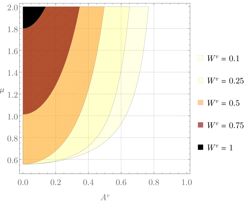
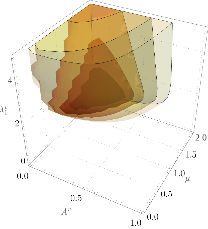
The feasibility regions of the inequality in Corollary 2 (i) are shown in Figure 3 for as a function of Avsuperscript𝐴𝑣A^{v}, μ𝜇\mu, and Wvsuperscript𝑊𝑣W^{v}, as well as the optimization variable λ1vsubscriptsuperscript𝜆𝑣1\lambda^{v}_{1}. Note that decreasing Wvsuperscript𝑊𝑣W^{v} and Avsuperscript𝐴𝑣A^{v} in Corollary 2 (i)-(ii) makes the left-hand side smaller which is an observation confirmed by Figure 3.
Refer to caption
(a) 3D feasibility region of Corollary 1 (i)
Refer to caption
(b) 2D cross-section of (a) for λ1v=1.80subscriptsuperscript𝜆𝑣11.80\lambda^{v}_{1}=1.80.
Figure 3: Feasibility regions of Corollary 1 (i) as a function of Avsuperscript𝐴𝑣A^{v}, λ1vsuperscriptsubscript𝜆1𝑣\lambda_{1}^{v}, μ𝜇\mu, and Wvsuperscript𝑊𝑣W^{v} for fixed K=10𝐾10K=10, Bv=1superscript𝐵𝑣1B^{v}=1 and λ2v=0superscriptsubscript𝜆2𝑣0\lambda_{2}^{v}=0. The plots were generated using the RegionPlot function of Mathematica.

This one-dimensional analysis provides valuable insights that we use to develop general tuning guidelines that favor the feasibility of the local LMI stability condition in (1). Specifically:

  1. (i)

    Decrease the magnitude of state weighting, i.e., reduce ρ(Wv)𝜌superscript𝑊𝑣\rho(W^{v}).

  2. (ii)

    Increase stability of the local dynamics, i.e., decrease ρ(Av)𝜌superscript𝐴𝑣\rho(A^{v}).

We will demonstrate how to apply these tuning guidelines through an illustrative example in the upcoming section.

VI Numerical case studies

VI-A Illustrative example: RHG can destabilize stable systems

Consider two agents with local dynamics of the form (30), with

A1=[0.60.30.30.7],B1=[105.5114],A2=[0.60.10.80.1],B2=[13196.510],formulae-sequencesuperscript𝐴1delimited-[]0.60.30.30.7formulae-sequencesuperscript𝐵1delimited-[]105.5114formulae-sequencesuperscript𝐴2delimited-[]0.60.10.80.1superscript𝐵2delimited-[]13196.510\displaystyle A^{1}=\left[\begin{smallmatrix}0.6&0.3\\ 0.3&0.7\end{smallmatrix}\right],\;B^{1}=\left[\begin{smallmatrix}10&5.5\\ 11&4\\ \end{smallmatrix}\right],\;A^{2}=\left[\begin{smallmatrix}0.6&0.1\\ 0.8&0.1\end{smallmatrix}\right],\;B^{2}=\left[\begin{smallmatrix}13&19\\ 6.5&10\\ \end{smallmatrix}\right],

yielding ρ(A1)=0.954𝜌superscript𝐴10.954\rho(A^{1})=0.954 and ρ(A2)=0.727𝜌superscript𝐴20.727\rho(A^{2})=0.727. Both agents have local state cost and an input coupling cost of the following form:

(xtv,utv,utv)=(xtv)Wv(xtv)+(j𝒱Rvuj)uvsuperscriptsubscript𝑥𝑡𝑣superscriptsubscript𝑢𝑡𝑣superscriptsubscript𝑢𝑡𝑣superscriptsuperscriptsubscript𝑥𝑡𝑣topsuperscript𝑊𝑣superscriptsubscript𝑥𝑡𝑣superscriptsubscript𝑗𝒱superscript𝑅𝑣superscript𝑢𝑗topsuperscript𝑢𝑣\displaystyle\ell(x_{t}^{v},u_{t}^{v},u_{t}^{-v})=(x_{t}^{v})^{\top}W^{v}(x_{t}^{v})+\Big{(}\sum_{j\in\mathcal{V}}R^{v}u^{j}\Big{)}^{\top}u^{v} (33)

where the parameters of the input cost are R1=blkdiag(10,0.01)superscript𝑅1blkdiag100.01R^{1}=\textrm{blkdiag}(10,0.01) and R2=blkdiag(0.01,20)superscript𝑅2blkdiag0.0120R^{2}=\textrm{blkdiag}(0.01,20). Cost functions with this structure characterize aggregative games [31], and appear in many resource allocation problems.

We simulate the resulting closed-loop system (15) using a prediction horizon of K=10𝐾10K=10, and different Wvsuperscript𝑊𝑣W^{v} matrices. Our findings are twofold. Firstly, we observe that the agents can destabilise each other by using RHG, even though the local dynamics are stable, as shown in Figure 4(a). This underscores the importance of our stability analyses and certificates. Secondly, we observe in Figure 4(b) that with a decreasing ρ(Wv)𝜌superscript𝑊𝑣\rho(W^{v}) the closed-loop dynamics become stable, in line with our tuning guidelines. Additionally, we observe that:

Refer to caption
(a) W1=diag(20,0.05),W2=diag(0.05,20)formulae-sequencesuperscript𝑊1diag200.05superscript𝑊2diag0.0520W^{1}=\text{diag}(20,0.05),W^{2}=\text{diag}(0.05,20), μ=0.498𝜇0.498\mu=0.498.
Refer to caption
(b) W1=diag(1,0.05),W2=diag(0.05,1)formulae-sequencesuperscript𝑊1diag10.05superscript𝑊2diag0.051W^{1}=\text{diag}(1,0.05),W^{2}=\text{diag}(0.05,1), μ=0.125𝜇0.125\mu=0.125.
Figure 4: Evolution of the closed-loop system in Section VI-A, for different choices of the state weighs Wvsuperscript𝑊𝑣W^{v} in the RHG feedback law.
  • In contrast to classical MPC, we observed in simulations that increasing the horizon length K𝐾K does not have a stabilizing effect for the closed-loop system under the RHG feedback law (15).

  • The feasibility of the LMI is negatively influenced not only by the magnitude of state and input weights, i.e., ρ(Rv),ρ(Wv)𝜌superscript𝑅𝑣𝜌superscript𝑊𝑣\rho(R^{v}),\;\rho(W^{v}), but also by their asymmetry across different agents.

  • The stable closed loop in Figures 4(b) stabilizes to the correspondent steady-state v-GNE (29), i.e, as t𝑡t\to\infty then xvx¯v=xsv=[0, 0]superscript𝑥𝑣superscript¯𝑥𝑣superscriptsubscript𝑥𝑠𝑣superscript0 0topx^{v}\to\bar{x}^{v}=x_{s}^{v}=[0,\leavevmode\nobreak\ 0]^{\top}. This supports our conjecture that agents find the operating point xssubscript𝑥𝑠x_{s} without terminal constraints.

Finally, our numerical studies highlight the conservative nature of the stability certificates. Specifically, we have observed instances where, despite violations of the stability certificates, the closed-loop systems remain stable. Moreover, while our analysis requires strong monotonicity of the pseudo-gradient, as postulated in Assumption 1(iii), the simulations reveal that stable closed-loop systems can be achieved even in scenarios with non-monotone pseudo-gradients.

VI-B Battery-charging game

In this section, we deploy RHG on a simplified version of the battery charging game presented in [33, 12].
Refer to caption
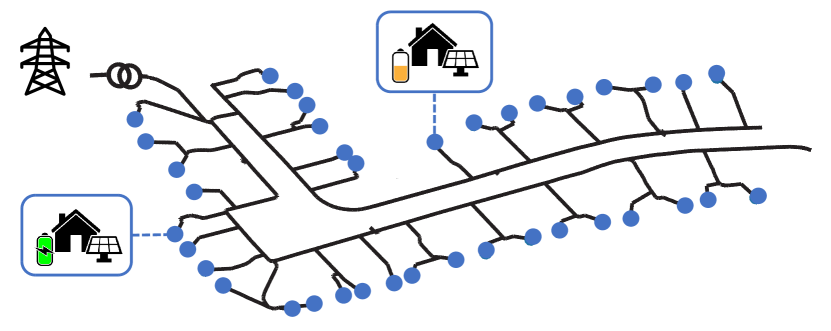
Figure 5: Schematic of households owning a private battery and being connected to the power grid through a point of common coupling.

VI-B1 Model

We consider a distribution grid composed of M𝑀M active consumers v𝒱={1,,M}𝑣𝒱1𝑀v\in\mathcal{V}=\{1,\dots,M\} connected to the main transmission grid via a point of common coupling, as is shown in Figure 5. Every consumer v𝒱𝑣𝒱v\in\mathcal{V} owns an energy storage device, or battery, with a controllable input utvsuperscriptsubscript𝑢𝑡𝑣u_{t}^{v} modeling charging if utv>0superscriptsubscript𝑢𝑡𝑣0u_{t}^{v}>0 and discharging if utv<0superscriptsubscript𝑢𝑡𝑣0u_{t}^{v}<0. Each consumer has an inflexible energy demand of dtvsubscriptsuperscript𝑑𝑣𝑡d^{v}_{t} units of power, at time t𝑡t, which they must fulfil by buying energy from the main grid ltv0superscriptsubscript𝑙𝑡𝑣subscriptabsent0l_{t}^{v}\in\mathbb{R}_{\geq 0} and/or discharging their local battery utvsuperscriptsubscript𝑢𝑡𝑣u_{t}^{v}. This requirement translate in the local energy-balance constraint

ltv=utv+dtv,v𝒱.formulae-sequencesuperscriptsubscript𝑙𝑡𝑣superscriptsubscript𝑢𝑡𝑣superscriptsubscript𝑑𝑡𝑣for-all𝑣𝒱\displaystyle l_{t}^{v}=u_{t}^{v}+d_{t}^{v},\quad\forall v\in\mathcal{V}. (34)

The power supplied to individual consumers is limited by

0ltvlmaxv,v𝒱,formulae-sequence0superscriptsubscript𝑙𝑡𝑣superscriptsubscript𝑙max𝑣for-all𝑣𝒱0\leq l_{t}^{v}\leq l_{\text{max}}^{v},\quad\forall v\in\mathcal{V}, (35)

where lmaxvsuperscriptsubscript𝑙max𝑣l_{\text{max}}^{v} is the maximum power a consumer can absorb from the main grid over the sampling period. Moreover, the charging/discharging control input utvsuperscriptsubscript𝑢𝑡𝑣u_{t}^{v} is constrained by the charging rate:

uminvutvumaxvsuperscriptsubscript𝑢min𝑣superscriptsubscript𝑢𝑡𝑣superscriptsubscript𝑢max𝑣\displaystyle u_{\text{min}}^{v}\leq u_{t}^{v}\leq u_{\text{max}}^{v} (36)

where umaxv0uminvsuperscriptsubscript𝑢max𝑣0superscriptsubscript𝑢min𝑣u_{\text{max}}^{v}\geq 0\geq u_{\text{min}}^{v} are the upper and lower charging limits. Thus, the local input constraint set (3a) is the following:

𝒰tv={utv| 0utv+dtvlmaxv,uminvutvumaxv}.superscriptsubscript𝒰𝑡𝑣conditional-setsubscriptsuperscript𝑢𝑣𝑡formulae-sequence 0superscriptsubscript𝑢𝑡𝑣superscriptsubscript𝑑𝑡𝑣superscriptsubscript𝑙max𝑣superscriptsubscript𝑢min𝑣superscriptsubscript𝑢𝑡𝑣superscriptsubscript𝑢max𝑣\displaystyle\mathcal{U}_{t}^{v}=\{u^{v}_{t}\leavevmode\nobreak\ |\leavevmode\nobreak\ 0\leq u_{t}^{v}+d_{t}^{v}\leq l_{\text{max}}^{v},\leavevmode\nobreak\ u_{\text{min}}^{v}\leq u_{t}^{v}\leq u_{\text{max}}^{v}\}.

Power line and transformer constraints at the point of common coupling limit the aggregate load of all consumers, as follows:

0v𝒱ltvLmax,0subscript𝑣𝒱superscriptsubscript𝑙𝑡𝑣subscript𝐿max0\leq\sum_{v\in\mathcal{V}}l_{t}^{v}\leq L_{\text{max}}, (37)

where Lmax>0subscript𝐿max0L_{\text{max}}>0 is the grid capacity. This constraint constitutes a coupling constraint, as in (3b). The correspondent constraint set is

𝒞t={(utv,utv)| 0v𝒱utv+dtvLmax}.subscript𝒞𝑡conditional-setsubscriptsuperscript𝑢𝑣𝑡subscriptsuperscript𝑢𝑣𝑡 0subscript𝑣𝒱superscriptsubscript𝑢𝑡𝑣superscriptsubscript𝑑𝑡𝑣subscript𝐿max\displaystyle\mathcal{C}_{t}=\left\{(u^{v}_{t},u^{-v}_{t})\leavevmode\nobreak\ \Big{|}\leavevmode\nobreak\ 0\leq\sum_{v\in\mathcal{V}}u_{t}^{v}+d_{t}^{v}\leq L_{\text{max}}\right\}.

Each battery has a scalar state-of-charge (SoC) xtvsuperscriptsubscript𝑥𝑡𝑣x_{t}^{v} evolving as

xt+1v=Avxtv+Bvutv,v𝒱,formulae-sequencesuperscriptsubscript𝑥𝑡1𝑣superscript𝐴𝑣superscriptsubscript𝑥𝑡𝑣superscript𝐵𝑣superscriptsubscript𝑢𝑡𝑣for-all𝑣𝒱\displaystyle x_{t+1}^{v}=A^{v}x_{t}^{v}+B^{v}u_{t}^{v},\quad\forall v\in\mathcal{V}, (38)

where Av,Bv[0,1]superscript𝐴𝑣superscript𝐵𝑣01A^{v},B^{v}\!\in\!\left[0,1\right] model leakage rate and charging efficiency.

We assume that each consumer v𝒱𝑣𝒱v\in\mathcal{V} is self-interested and aims to minimize its electricity bill as well as the operational cost of its battery, yielding a local cost function of the form

tv(xtv,utv,utv)=(γ1,tvj𝒱ltj+γ2,tv)ltvenergy cost+γ3,tv(xtvxref)2battery usage,superscriptsubscript𝑡𝑣subscriptsuperscript𝑥𝑣𝑡subscriptsuperscript𝑢𝑣𝑡superscriptsubscript𝑢𝑡𝑣subscriptsuperscriptsubscript𝛾1𝑡𝑣subscript𝑗𝒱superscriptsubscript𝑙𝑡𝑗superscriptsubscript𝛾2𝑡𝑣superscriptsubscript𝑙𝑡𝑣energy costsubscriptsuperscriptsubscript𝛾3𝑡𝑣superscriptsubscriptsuperscript𝑥𝑣𝑡superscript𝑥ref2battery usage\displaystyle\ell_{t}^{v}(x^{v}_{t},u^{v}_{t},u_{t}^{-v})=\,\underbrace{\left(\gamma_{1,t}^{v}\sum_{j\in\mathcal{V}}l_{t}^{j}+\gamma_{2,t}^{v}\right)\,l_{t}^{v}}_{\text{energy cost}}+\underbrace{\gamma_{3,t}^{v}\,(x^{v}_{t}-x^{\text{ref}})^{2}}_{\text{battery usage}},

where ltv=utv+dtvsuperscriptsubscript𝑙𝑡𝑣superscriptsubscript𝑢𝑡𝑣superscriptsubscript𝑑𝑡𝑣l_{t}^{v}=u_{t}^{v}+d_{t}^{v} as defined in (34). This stage cost follows the general structure in (2). The constants γ1,tv,γ2,tv>0superscriptsubscript𝛾1𝑡𝑣superscriptsubscript𝛾2𝑡𝑣0\gamma_{1,t}^{v},\gamma_{2,t}^{v}>0 represent different price rates that consumers previously negotiated with suppliers. The second term, with γ3,t>0subscript𝛾3𝑡0\gamma_{3,t}>0, reflects agent v𝑣v’s aim to maintain its battery charge state near the reference xrefsuperscript𝑥refx^{\text{ref}} to minimize degradation.

VI-B2 Implementation

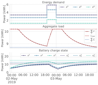
We consider a battery charging game between 3 heterogeneous consumers owning similar storage devices, i.e., a lithium-ion battery with SoC dynamics as in (38) and parameters Av[0.955,0.98]superscript𝐴𝑣0.9550.98A^{v}\in[0.955,0.98] (corresponding to a leakage rate of about 0.8 over the 24 hours) and Bv[0.7,0.9]superscript𝐵𝑣0.70.9B^{v}\in[0.7,0.9], as in [33], umaxv=uminv=7superscriptsubscript𝑢max𝑣superscriptsubscript𝑢min𝑣7u_{\text{max}}^{v}=-u_{\text{min}}^{v}=7 kWh, and xref[15,20]superscript𝑥ref1520x^{\text{ref}}\in[15,20] kWh. The price rates are γ1v[0.03,0.05]subscriptsuperscript𝛾𝑣10.030.05\gamma^{v}_{1}\in[0.03,0.05] $/kWh for the coupling price, γ2v[0.01,0.2]subscriptsuperscript𝛾𝑣20.010.2\gamma^{v}_{2}\in[0.01,0.2] $/kWh, for the base energy price, and γ3v[0.01,0.02]superscriptsubscript𝛾3𝑣0.010.02\gamma_{3}^{v}\in[0.01,0.02] for battery usage weight. For the demand profiles dtvsubscriptsuperscript𝑑𝑣𝑡d^{v}_{t}, we used real data from single-family homes situated in the state of New York collected on the 2nd of May 2019 and averaged over 48 hours [34]. Additionally, we apply an energy demand shock which doubles the base demand dtvsuperscriptsubscript𝑑𝑡𝑣d_{t}^{v} of all agents between 9 pm and 1 am. After successfully verifying closed-loop stability using the local LMI-based certificates in Corollary 1, we simulate this battery charging game under RHG control over 48 hours, and illustrate the results in Figure 6. All simulations are implemented in Python, and the v-GNE is computed using a Smoothed Fischer-Burmeister method [35].
Refer to caption
Figure 6: Evolution of the energy demand (top), aggregagate load (center), and battery state of charge (bottom) for the 3-consumer charging game in Section VI-B under the RHG feedback law.

VI-B3 Discussion

The simulation study demonstrates three things: (i) The distributed stability check in Corollary 1 effectively guarantees closed-loop stability, (ii) the consumers stabilize to the steady-state v-GNE (29), as conjectured; (iii) the aggregate load constraint (37) can be enforced despite unforeseen disturbances. Before the demand shock, all consumer charge their batteries, so that the SoC converges to a close neighborhood of the steady-state v-GNE xsvsuperscriptsubscript𝑥𝑠𝑣x_{s}^{v} (29), as shown in Fig. 6 (bottom). During the demand shock, the agents buy from the grid and discharge their batteries to serve their increased demand. Note that the aggregate load constraint is successfully enforced, albeit agents have no preview of the shock. After the demand shock, states and inputs re-stabilize to their respective steady states.

VII Conclusion

This paper presents LMI-based stability certificates for game-theoretic MPC, specifically for strongly monotone games with coupling in the cost and the constraints played in receding horizon. Our certificates can be numerically verified to show global asymptotic stability. Moreover, if the agents have decoupled dynamics, the certificates can be evaluated locally, therefore offering a simple path towards verifying asymptotic stability for games with a large number of agents. We demonstrate the usefulness of RHG and the effectiveness of our certificates in a battery charging game. In future works, we will focus on the development of terminal ingredients to enforce closed-loop stability for unstable LTI systems.

References

  • [1] T. Roughgarden and E. Tardos, “How bad is selfish routing?,” Journal of the ACM, vol. 49, pp. 236–259, Mar. 2002.
  • [2] S. Matthewman and H. Byrd, “Blackouts: a sociology of electrical power failure,” 2014.
  • [3] H. S. Gordon, “The economic theory of a common-property resource: the fishery,” Journal of Polit. Econ., vol. 62, no. 2, pp. 124–142, 1954.
  • [4] M. A. Müller and F. Allgöwer, “Economic and distributed model predictive control: Recent developments in optimization-based control,” SICE Journal of Control, Measurement, and System Integration, vol. 10, pp. 39–52, Mar. 2017.
  • [5] G. Hardin, “The tragedy of the commons: The population problem has no technical solution; it requires a fundamental extension in morality.,” Science, vol. 162, pp. 1243–1248, Dec. 1968.
  • [6] E. Koutsoupias and C. Papadimitriou, “Worst-case equilibria,” in Annual symposium on theoretical aspects of computer science, pp. 404–413, Springer, 1999.
  • [7] G. Belgioioso, P. Yi, S. Grammatico, and L. Pavel, “Distributed generalized Nash equilibrium seeking: An operator-theoretic perspective,” IEEE Control Systems Magazine, vol. 42, pp. 87–102, aug 2022.
  • [8] M. Köhler, L. Krügel, L. Grüne, M. A. Müller, and F. Allgöwer, “Transient performance of mpc for tracking,” IEEE Control Systems Letters, vol. 7, pp. 2545–2550, 2023.
  • [9] E. Mazumdar, L. J. Ratliff, and S. S. Sastry, “On gradient-based learning in continuous games,” SIAM J. Math. Data Sci., vol. 2, no. 1, pp. 103–131, 2020.
  • [10] B. Nortmann, A. Monti, M. Sassano, and T. Mylvaganam, “Nash equilibria for linear quadratic discrete-time dynamic games via iterative and data-driven algorithms,” IEEE Trans. Autom. Control, 2024.
  • [11] F. Laine, D. Fridovich-Keil, C.-Y. Chiu, and C. Tomlin, “The computation of approximate generalized feedback Nash equilibria,” SIAM J. Optim., vol. 33, no. 1, pp. 294–318, 2023.
  • [12] S. Hall, G. Belgioioso, D. Liao-McPherson, and F. Dorfler, “Receding horizon games with coupling constraints for demand-side management,” in 2022 IEEE 61st Conference on Decision and Control (CDC), pp. 3795–3800, 2022.
  • [13] R. Spica, E. Cristofalo, Z. Wang, E. Montijano, and M. Schwager, “A real-time game theoretic planner for autonomous two-player drone racing,” IEEE Trans. Robot., vol. 36, pp. 1389–1403, Oct. 2020.
  • [14] M. Wang, Z. Wang, J. Talbot, J. C. Gerdes, and M. Schwager, “Game-theoretic planning for self-driving cars in multivehicle competitive scenarios,” IEEE Transactions on Robotics, pp. 1–13, 2021.
  • [15] S. Hall, L. Guerrini, F. Dörfler, and D. Liao-McPherson, “Game-theoretic model predictive control for modelling competitive supply chains,” arXiv preprint arXiv:2401.09853, 2024.
  • [16] D. Gu, “A differential game approach to formation control,” IEEE Trans. Control Syst. Technol., vol. 16, pp. 85–93, Jan. 2008.
  • [17] A. Liniger and J. Lygeros, “A noncooperative game approach to autonomous racing,” IEEE Transactions on Control Systems Technology, vol. 28, pp. 884–897, May 2020.
  • [18] S. Le Cleac’h, M. Schwager, and Z. Manchester, “Algames: a fast augmented lagrangian solver for constrained dynamic games,” Autonomous Robots, vol. 46, no. 1, pp. 201–215, 2022.
  • [19] N. Mignoni, R. Carli, and M. Dotoli, “Distributed noncooperative mpc for energy scheduling of charging and trading electric vehicles in energy communities,” IEEE Transactions on Control Systems Technology, 2023.
  • [20] A. D. Paola, F. Fele, D. Angeli, and G. Strbac, “Distributed coordination of price-responsive electric loads: A receding horizon approach,” in 2018 IEEE Conference on Decision and Control (CDC), IEEE, dec 2018.
  • [21] E. Benenati and S. Grammatico, “Probabilistic game-theoretic traffic routing,” arXiv preprint arXiv:2303.03295, 2023.
  • [22] A. N. Venkat, J. B. Rawlings, and S. J. Wright, “Stability and optimality of distributed model predictive control,” in Proceedings of the 44th IEEE Conference on Decision and Control, pp. 6680–6685, IEEE, 2005.
  • [23] F. Fabiani and A. Simonetto, “Incentives and co-evolution: Steering linear dynamical systems with noncooperative agents,” IEEE Trans. Control Netw. Syst., pp. 1–12, 2023.
  • [24] F. Facchinei and C. Kanzow, “Generalized Nash equilibrium problems,” 4OR, vol. 5, no. 3, pp. 173–210, 2009.
  • [25] F. Facchinei and J. Pang, “Nash equilibria: the variational approach,” in Convex Optimization in Signal Processing and Communications, pp. 443–493, Cambridge University Press, dec 2009.
  • [26] H. H. Bauschke and P. L. Combettes, Convex Analysis and Monotone Operator Theory in Hilbert Spaces. Springer, 2017.
  • [27] F. Facchinei and J. Pang, Finite-Dimensional Variational Inequalities and Complementarity Problems. Springer Series in Operations Research and Financial Engineering, Springer New York, 2007.
  • [28] L. Grüne and J. Pannek, Nonlinear Model Predictive Control. Springer London, 2011.
  • [29] S. Diamond and S. Boyd, “CVXPY: A Python-embedded modeling language for convex optimization,” Journal of Machine Learning Research, vol. 17, no. 83, pp. 1–5, 2016.
  • [30] T. Faulwasser, L. Grüne, and M. A. Müller, “Economic nonlinear model predictive control,” Foundations and Trends® in Systems and Control, vol. 5, no. 1, pp. 1–98, 2018.
  • [31] G. Belgioioso and S. Grammatico, “On convexity and monotonicity in generalized aggregative games,” IFAC-PapersOnLine, vol. 50, no. 1, pp. 14338–14343, 2017. 20th IFAC World Congress.
  • [32] G. Scutari, F. Facchinei, J.-S. Pang, and D. P. Palomar, “Real and complex monotone communication games,” IEEE Transactions on Information Theory, vol. 60, pp. 4197–4231, July 2014.
  • [33] I. Atzeni, L. G. Ordóñez, G. Scutari, D. P. Palomar, and J. R. Fonollosa, “Demand-side management via distributed energy generation and storage optimization,” IEEE Trans. Smart Grid, vol. 4, pp. 866–876, June 2012.
  • [34] Pecan Street Datport, “Residential data new york.” [online], Mar. 2022.
  • [35] D. Liao-McPherson, M. Huang, and I. Kolmanovsky, “A regularized and smoothed fischer–burmeister method for quadratic programming with applications to model predictive control,” IEEE Transactions on Automatic Control, vol. 64, pp. 2937–2944, July 2019.
  • [36] W. M. Haddad and V. Chellaboina, Stability and Dissipativity Theory for Discrete-Time Nonlinear Dynamical Systems, pp. 763–844. Princeton University Press, 2008.
  • [37] S. A. Morris, “The schauder-tychonoff fixed point theorem and applications,” Matematickỳ časopis, vol. 25, no. 2, pp. 165–172, 1975.
  • [38] G. C. Goodwin, J. A. D. Doná, and M. M. Seron, Constrained Control and Estimation. Springer London, 2005.

Appendix A Appendix

A-A Proof of Theorem 1

We start by writing the pseudo-gradient (17) more explicitly as

F(u,𝐱)=Fu(u)+Fx𝐱,𝐹𝑢𝐱subscript𝐹𝑢𝑢subscript𝐹𝑥𝐱\displaystyle F(u,\mathbf{x})=F_{u}(u)+F_{x}\mathbf{x}, (39)

where the component mappings are defined as

Fu(u)=[u1u1(u1,u1)uMuv(uM,uM)]subscript𝐹𝑢𝑢delimited-[]subscriptsuperscript𝑢1superscriptsubscript𝑢1superscript𝑢1superscript𝑢1subscriptsuperscript𝑢𝑀superscriptsubscript𝑢𝑣superscript𝑢𝑀superscript𝑢𝑀\displaystyle F_{u}(u)=\left[\begin{smallmatrix}\partial_{u^{1}}\ell_{u}^{1}(u^{1},u^{-1})\\ \vdots\\ \partial_{u^{M}}\ell_{u}^{v}(u^{M},u^{-M})\end{smallmatrix}\right]
+[2(B~1)W~1B~1(B~1)W~1B~M(B~M)W~MB~M2(B~M)W~MB~M]u+[(B~1)w~1(B~M)w~M]delimited-[]2superscriptsuperscript~𝐵1topsuperscript~𝑊1superscript~𝐵1superscriptsuperscript~𝐵1topsuperscript~𝑊1superscript~𝐵𝑀superscriptsuperscript~𝐵𝑀topsuperscript~𝑊𝑀superscript~𝐵𝑀2superscriptsuperscript~𝐵𝑀topsuperscript~𝑊𝑀superscript~𝐵𝑀𝑢delimited-[]superscriptsuperscript~𝐵1topsuperscript~𝑤1superscriptsuperscript~𝐵𝑀topsuperscript~𝑤𝑀\displaystyle+\left[\begin{smallmatrix}2(\tilde{B}^{1})^{\top}\tilde{W}^{1}\tilde{B}^{1}&\ldots&(\tilde{B}^{1})^{\top}\tilde{W}^{1}\tilde{B}^{M}\\ \vdots&\ddots&\vdots\\ (\tilde{B}^{M})^{\top}\tilde{W}^{M}\tilde{B}^{M}&\ldots&2(\tilde{B}^{M})^{\top}\tilde{W}^{M}\tilde{B}^{M}\end{smallmatrix}\right]u+\left[\begin{smallmatrix}(\tilde{B}^{1})^{\top}\tilde{w}^{1}\\ \vdots\\ (\tilde{B}^{M})^{\top}\tilde{w}^{M}\end{smallmatrix}\right] (40)
Fx=[2(B~1)W~1A~2(B~M)W~MA~].subscript𝐹𝑥delimited-[]2superscriptsuperscript~𝐵1topsuperscript~𝑊1~𝐴2superscriptsuperscript~𝐵𝑀topsuperscript~𝑊𝑀~𝐴\displaystyle F_{x}=\left[\begin{smallmatrix}2(\tilde{B}^{1})^{\top}\tilde{W}^{1}\tilde{A}\\ \vdots\\ 2(\tilde{B}^{M})^{\top}\tilde{W}^{M}\tilde{A}\end{smallmatrix}\right]. (41)

with A~~𝐴\tilde{A} being the free response matrix of the global dynamics (1), and B~vsuperscript~𝐵𝑣\tilde{B}^{v} the impulse response matrix of agent v𝑣v, namely,

A~=[IA(A)K],B~v=[00Bv00ABvBv00(A)K1BvABvBv],formulae-sequence~𝐴delimited-[]𝐼𝐴superscript𝐴𝐾superscript~𝐵𝑣delimited-[]00superscript𝐵𝑣00𝐴superscript𝐵𝑣superscript𝐵𝑣00superscript𝐴𝐾1superscript𝐵𝑣𝐴superscript𝐵𝑣superscript𝐵𝑣\displaystyle\tilde{A}=\left[\begin{smallmatrix}I\\ A\\ \vdots\\ (A)^{K}\end{smallmatrix}\right],\quad\tilde{B}^{v}=\left[\begin{smallmatrix}0&\cdots&\cdots&0\\ B^{v}&0&\cdots&0\\ AB^{v}&B^{v}&\cdots&0\\ \vdots&\ddots&\ddots&0\\ (A)^{K-1}B^{v}&\cdots&AB^{v}&B^{v}\end{smallmatrix}\right], (42)

and, further, W~v=blkdiag(Wv,,Wv),w~v=col(wv,,wv)formulae-sequencesuperscript~𝑊𝑣blkdiagsuperscript𝑊𝑣superscript𝑊𝑣superscript~𝑤𝑣colsuperscript𝑤𝑣superscript𝑤𝑣\tilde{W}^{v}=\text{blkdiag}(W^{v},\dots,W^{v}),\;\tilde{w}^{v}=\text{col}(w^{v},\dots,w^{v}). The proof of Theorem 1 consists of four main parts. 1) Showing existence of the equilibrium point x¯¯𝑥\bar{x}, 2) Deriving dissipativity inequalities for Σ1subscriptΣ1\Sigma_{1} and Σ2subscriptΣ2\Sigma_{2}, 3) Interconnecting the two subsystems, 4) Invoking [36, Th. 13.2] to verify that the sum of storage functions of the two subsystems fulfills the conditions for a Lyapunov function.

1) We begin by showing that the set of equilibrium points for (16), ={x¯|x¯=Ax¯+Bκ(x¯)}conditional-set¯𝑥¯𝑥𝐴¯𝑥𝐵𝜅¯𝑥\mathcal{E}=\{\bar{x}\leavevmode\nobreak\ |\leavevmode\nobreak\ \bar{x}=A\bar{x}+B\kappa(\bar{x})\}, is non-empty by using a fixed point theorem [37]. Rearranging the definition of \mathcal{E}, we define the mapping z(x)=(IA)1Bκ(x)𝑧𝑥superscript𝐼𝐴1𝐵𝜅𝑥z(x)=(I-A)^{-1}B\kappa(x) which: (i) is single-valued (as ρ(A)<1𝜌𝐴1\rho(A)<1 by Assumption 1 (i)), (ii) has the same set of fixed-points as the closed-loop dynamics (16), (iii) is continuous by Proposition 2 and (iv) maps onto the set {z|(IA)z=Bu,u𝒵}conditional-set𝑧formulae-sequence𝐼𝐴𝑧𝐵𝑢𝑢𝒵\{z\leavevmode\nobreak\ |\leavevmode\nobreak\ (I-A)z=Bu,\leavevmode\nobreak\ \leavevmode\nobreak\ u\in\mathcal{Z}\} which is compact as 𝒵𝒵\mathcal{Z} (defined in (11)) is compact under Assumption 1 (ii). Hence, we can apply the Schauder-Tychonoff fixed-point theorem [37] to conclude existence of at least one fixed point x¯¯𝑥\bar{x}\in\mathcal{E} of z(x)𝑧𝑥z(x) which is also an equilibrium point of (16).

2) Next, we derive dissipation inequalities with storage functions V1subscript𝑉1V_{1} and V2subscript𝑉2V_{2} for each subsystem Σ1subscriptΣ1\Sigma_{1} (22) and Σ2subscriptΣ2\Sigma_{2} (23) separately. We define Δxt=(xtx¯)Δsubscript𝑥𝑡subscript𝑥𝑡¯𝑥\Delta x_{t}=(x_{t}-\bar{x}), Δyt,i=(yt,iy¯i)Δsubscript𝑦𝑡𝑖subscript𝑦𝑡𝑖subscript¯𝑦𝑖\Delta y_{t,i}=(y_{t,i}-\bar{y}_{i}), and Δut,i=(ut,iu¯i),i{1,2}formulae-sequenceΔsubscript𝑢𝑡𝑖subscript𝑢𝑡𝑖subscript¯𝑢𝑖𝑖12\Delta u_{t,i}=(u_{t,i}-\bar{u}_{i}),\leavevmode\nobreak\ i\in\{1,2\}.
As Σ1subscriptΣ1\Sigma_{1} is a discrete-time LTI system, we choose a quadratic storage function family as Vx¯1(xt)=(Δxt)P(Δxt)subscriptsuperscript𝑉1¯𝑥subscript𝑥𝑡superscriptΔsubscript𝑥𝑡top𝑃Δsubscript𝑥𝑡V^{1}_{\bar{x}}(x_{t})=(\Delta x_{t})^{\top}P\leavevmode\nobreak\ (\Delta x_{t}), for some positive definite P𝑃P. Evaluating the evolution of Vx¯1subscriptsuperscript𝑉1¯𝑥V^{1}_{\bar{x}} along trajectories gives

Vx¯1(xt+1)Vx¯1(xt)=[Δy1,tΔu1,t][APAPAPBBPB][Δy1,tΔu1,t]subscriptsuperscript𝑉1¯𝑥subscript𝑥𝑡1subscriptsuperscript𝑉1¯𝑥subscript𝑥𝑡superscriptmatrixΔsubscript𝑦1𝑡Δsubscript𝑢1𝑡topmatrixsuperscript𝐴top𝑃𝐴𝑃superscript𝐴top𝑃𝐵superscript𝐵top𝑃𝐵matrixΔsubscript𝑦1𝑡Δsubscript𝑢1𝑡V^{1}_{\bar{x}}(x_{t+1})-V^{1}_{\bar{x}}(x_{t})=\\ \begin{bmatrix}\Delta y_{1,t}\\ \Delta u_{1,t}\end{bmatrix}^{\top}\begin{bmatrix}A^{\top}PA-P&A^{\top}PB\\ *&B^{\top}PB\\ \end{bmatrix}\begin{bmatrix}\Delta y_{1,t}\\ \Delta u_{1,t}\end{bmatrix} (43)

By Proposition 2, the static nonlinearity ϕ()italic-ϕ\phi(\cdot) in (23) is μ𝜇\mu-cocoercive and 1μ1𝜇\frac{1}{\mu}-Lipschitz, and thus obeys the following inequalities:

Vx¯2=0subscriptsuperscript𝑉2¯𝑥0absent\displaystyle V^{2}_{\bar{x}}=0\leq [Δyt,2Δut,2][μI12I0][Δyt,2Δut,2],superscriptmatrixΔsubscript𝑦𝑡2Δsubscript𝑢𝑡2topmatrix𝜇𝐼12𝐼0matrixΔsubscript𝑦𝑡2Δsubscript𝑢𝑡2\displaystyle\begin{bmatrix}\Delta y_{t,2}\\ \Delta u_{t,2}\end{bmatrix}^{\top}\begin{bmatrix}-\mu I&\frac{1}{2}I\\ *&0\end{bmatrix}\begin{bmatrix}\Delta y_{t,2}\\ \Delta u_{t,2}\end{bmatrix}, (44)
Vx¯2=0subscriptsuperscript𝑉2¯𝑥0absent\displaystyle V^{2}_{\bar{x}}=0\leq [Δyt,2Δut,2][I01μ2I][Δyt,2Δut,2].superscriptmatrixΔsubscript𝑦𝑡2Δsubscript𝑢𝑡2topmatrix𝐼01superscript𝜇2𝐼matrixΔsubscript𝑦𝑡2Δsubscript𝑢𝑡2\displaystyle\begin{bmatrix}\Delta y_{t,2}\\ \Delta u_{t,2}\end{bmatrix}^{\top}\begin{bmatrix}-I&0\\ *&\frac{1}{\mu^{2}}I\end{bmatrix}\begin{bmatrix}\Delta y_{t,2}\\ \Delta u_{t,2}\end{bmatrix}. (45)

We take the conic combination of (44) and (45) which yields:

00absent\displaystyle 0\leq [Δyt,2Δut,2](λ1[μI12I0]+λ2[I01μ2I])[Δyt,2Δut,2],superscriptmatrixΔsubscript𝑦𝑡2Δsubscript𝑢𝑡2topsubscript𝜆1matrix𝜇𝐼12𝐼0subscript𝜆2matrix𝐼01superscript𝜇2𝐼matrixΔsubscript𝑦𝑡2Δsubscript𝑢𝑡2\displaystyle\begin{bmatrix}\Delta y_{t,2}\\ \Delta u_{t,2}\end{bmatrix}^{\top}\left(\lambda_{1}\begin{bmatrix}-\mu I&\frac{1}{2}I\\ *&0\end{bmatrix}+\lambda_{2}\begin{bmatrix}-I&0\\ *&\frac{1}{\mu^{2}}I\end{bmatrix}\right)\begin{bmatrix}\Delta y_{t,2}\\ \Delta u_{t,2}\end{bmatrix}, (46)

where λ10subscript𝜆10\lambda_{1}\geq 0 and λ20subscript𝜆20\lambda_{2}\geq 0 are scalars satisfying λ1+λ2>0subscript𝜆1subscript𝜆20\lambda_{1}+\lambda_{2}>0.

3) To analyze the interconnection of the two systems we recall that

Δu1,t=ΞΔy2,tΔsubscript𝑢1𝑡ΞΔsubscript𝑦2𝑡\displaystyle\Delta u_{1,t}=\Xi\leavevmode\nobreak\ \Delta y_{2,t} (47)
Δu2,t=FxΔy1,t.Δsubscript𝑢2𝑡subscript𝐹𝑥Δsubscript𝑦1𝑡\displaystyle\Delta u_{2,t}=-F_{x}\leavevmode\nobreak\ \Delta y_{1,t}. (48)

By substituting (47) into (43) and (48) into (46), we can write both inequalities in terms of the outputs Δy1,tΔsubscript𝑦1𝑡\Delta y_{1,t} and Δy2,tΔsubscript𝑦2𝑡\Delta y_{2,t}, and add them together which gives

Vx¯(xt+1)Vx¯(xt)=subscript𝑉¯𝑥subscript𝑥𝑡1subscript𝑉¯𝑥subscript𝑥𝑡absent\displaystyle V_{\bar{x}}(x_{t+1})-V_{\bar{x}}(x_{t})= Vx¯1(xt+1)Vx¯1(xt)+0subscriptsuperscript𝑉1¯𝑥subscript𝑥𝑡1subscriptsuperscript𝑉1¯𝑥subscript𝑥𝑡0\displaystyle\,V^{1}_{\bar{x}}(x_{t+1})-V^{1}_{\bar{x}}(x_{t})+0
=\displaystyle= [Δy1,tΔy2,t]([APAPAPB^B^PB^]\displaystyle\begin{bmatrix}\Delta y_{1,t}\\ \Delta y_{2,t}\end{bmatrix}^{\top}\left(\begin{bmatrix}A^{\top}PA-P&A^{\top}P\hat{B}\\ *&\hat{B}^{\top}P\hat{B}\\ \end{bmatrix}\right.
+[λ2μ2FxFxλ12Fx(λ1μ+λ2)I])[Δy1,tΔy2,t],\displaystyle+\left.\begin{bmatrix}\frac{\lambda_{2}}{\mu^{2}}F_{x}^{\top}F_{x}&-\frac{\lambda_{1}}{2}F_{x}^{\top}\\ *&-(\lambda_{1}\mu+\lambda_{2})I\end{bmatrix}\right)\begin{bmatrix}\Delta y_{1,t}\\ \Delta y_{2,t}\end{bmatrix},

where B^=BΞ^𝐵𝐵Ξ\hat{B}=B\leavevmode\nobreak\ \Xi. Thus, if

[APAPAPB^B^PB^]+[λ2μ2FxFxλ12Fx(λ1μ+λ2)I]ϵIprecedes-or-equalsmatrixsuperscript𝐴top𝑃𝐴𝑃superscript𝐴top𝑃^𝐵superscript^𝐵top𝑃^𝐵matrixsubscript𝜆2superscript𝜇2superscriptsubscript𝐹𝑥topsubscript𝐹𝑥subscript𝜆12superscriptsubscript𝐹𝑥topsubscript𝜆1𝜇subscript𝜆2𝐼italic-ϵ𝐼\displaystyle\begin{bmatrix}A^{\top}PA-P&A^{\top}P\hat{B}\\ *&\hat{B}^{\top}P\hat{B}\\ \end{bmatrix}+\begin{bmatrix}\frac{\lambda_{2}}{\mu^{2}}F_{x}^{\top}F_{x}&-\frac{\lambda_{1}}{2}F_{x}^{\top}\\ *&-(\lambda_{1}\mu+\lambda_{2})I\end{bmatrix}\preceq-\epsilon\,I (49)

for some ϵ>0italic-ϵ0\epsilon>0, then Vx¯(xt+1)Vx¯(xt)<0subscript𝑉¯𝑥subscript𝑥𝑡1subscript𝑉¯𝑥subscript𝑥𝑡0V_{\bar{x}}(x_{t+1})-V_{\bar{x}}(x_{t})<0.

4) To show closed-loop stability of the interconnected system, we apply the discrete-time Lyapunov theorem [36, Thrm. 13.2]. To invoke this result, the following conditions must be satisfied: (i) Vx¯(x¯)=0subscript𝑉¯𝑥¯𝑥0V_{\bar{x}}(\bar{x})=0, (ii) Vx¯(x)>0,xnx\{x¯}formulae-sequencesubscript𝑉¯𝑥𝑥0for-all𝑥\superscriptsubscript𝑛𝑥¯𝑥V_{\bar{x}}(x)>0,\;\forall x\in\mathbb{R}^{n_{x}}\backslash\{\bar{x}\}, (iii) Vx¯(x)subscript𝑉¯𝑥𝑥V_{\bar{x}}(x)\to\leavevmode\nobreak\ \infty as xnorm𝑥\|x\|\to\infty, (iv) Vx¯(f(x))Vx¯(x)< 0,subscript𝑉¯𝑥𝑓𝑥subscript𝑉¯𝑥𝑥 0V_{\bar{x}}(f(x))-V_{\bar{x}}(x)<\leavevmode\nobreak\ 0, xnxfor-all𝑥superscriptsubscript𝑛𝑥\forall x\in\mathbb{R}^{n_{x}}. Requirements (i)-(iii) hold as the candidate function is defined as Vx¯(xt)=ΔxPΔxsubscript𝑉¯𝑥subscript𝑥𝑡Δsuperscript𝑥top𝑃Δ𝑥V_{\bar{x}}(x_{t})=\Delta x^{\top}P\Delta x with P𝒮0nx𝑃superscriptsubscript𝒮succeedsabsent0subscript𝑛𝑥P\in\mathcal{S}_{\succ 0}^{n_{x}}, and (iv) is satisfied as we impose the decrease in (49). Therefore, all conditions of [36, Thrm. 13.2] are fulfilled and the equilibrium point x¯¯𝑥\bar{x} is globally asymptotically stable for ϵ>0italic-ϵ0\epsilon>0 and stable if ϵ=0italic-ϵ0\epsilon=0. Input constraint satisfaction is always ensured by the solution of the OCP in (10) and the problem is recursively feasible 𝐱nxfor-all𝐱superscriptsubscript𝑛𝑥\forall\,\mathbf{x}\in\mathbb{R}^{n_{x}} as we have no state constraints.

A-B Proof of Proposition 3

We want to prove that the steady-state v-GNE xssubscript𝑥𝑠x_{s} in (29) is the unique equilibrium point of the closed-loop system (16), i.e., xs=Axs+Bκs(xs)subscript𝑥𝑠𝐴subscript𝑥𝑠𝐵subscript𝜅𝑠subscript𝑥𝑠x_{s}=A\,x_{s}+B\,\kappa_{s}(x_{s}), where κs(x)subscript𝜅𝑠𝑥\kappa_{s}(x) is the associated steady-state feedback law of the following RHG scheme

minx,uvsubscript𝑥superscript𝑢𝑣\displaystyle\min_{x,u^{v}} k=0K1xkWxk+uv(ukv,usv)superscriptsubscript𝑘0𝐾1superscriptsubscript𝑥𝑘top𝑊subscript𝑥𝑘superscriptsubscript𝑢𝑣subscriptsuperscript𝑢𝑣𝑘superscriptsubscript𝑢𝑠𝑣\displaystyle\sum_{k=0}^{K-1}x_{k}^{\top}Wx_{k}+\ell_{u}^{v}(u^{v}_{k},u_{s}^{-v})
s.t. xk+1=Axk+Bvukv+Bvusv,kKformulae-sequencesubscript𝑥𝑘1𝐴subscript𝑥𝑘superscript𝐵𝑣superscriptsubscript𝑢𝑘𝑣superscript𝐵𝑣superscriptsubscript𝑢𝑠𝑣𝑘subscript𝐾\displaystyle\quad x_{k+1}=A\,x_{k}+B^{v}\,u_{k}^{v}+B^{-v}u_{s}^{-v},\quad k\in\mathbb{Z}_{K} (50a)
(ukv,usv)𝒵,kKformulae-sequencesuperscriptsubscript𝑢𝑘𝑣superscriptsubscript𝑢𝑠𝑣𝒵𝑘subscript𝐾\displaystyle\quad(u_{k}^{v},u_{s}^{-v})\in\mathcal{Z},\hskip 93.00017ptk\in\mathbb{Z}_{K} (50b)
x0=xs,xK=xs,formulae-sequencesubscript𝑥0subscript𝑥𝑠subscript𝑥𝐾subscript𝑥𝑠\displaystyle\quad x_{0}=x_{s},x_{K}=x_{s}, (50c)

which is the same as (10) but with an additional terminal state constraint xK=xssubscript𝑥𝐾subscript𝑥𝑠x_{K}=x_{s}.

The proof consists of two main parts: 1) We derive the KKT conditions of the steady-state game (29) and evaluate them at the proposed equilibrium point (xs,us)subscript𝑥𝑠subscript𝑢𝑠(x_{s},u_{s}). 2) We derive the KKT conditions of (50) and show that ukv=usv,λk=λs,kKformulae-sequencesubscriptsuperscript𝑢𝑣𝑘subscriptsuperscript𝑢𝑣𝑠formulae-sequencesubscript𝜆𝑘subscript𝜆𝑠for-all𝑘subscript𝐾u^{v}_{k}=u^{v}_{s},\,\lambda_{k}=\lambda_{s},\,\forall\,k\in\mathbb{Z}_{K} and xk=xs,subscript𝑥𝑘subscript𝑥𝑠x_{k}=x_{s},kK+1for-all𝑘subscript𝐾1\forall\,k\in\mathbb{Z}_{K+1} is the unique v-GNE trajectory satisfying them and thus κs(xs)=ussubscript𝜅𝑠subscript𝑥𝑠subscript𝑢𝑠\kappa_{s}(x_{s})=u_{s}. Since usint𝒵subscript𝑢𝑠int𝒵u_{s}\in\text{int}\,\mathcal{Z} by assumption, we can neglect the inequality constraints in (50b) moving forward.

1) We begin by noting that under Assumption 1(iii), the pseudo-gradient mapping of (29) is strongly monotone and thus the solution of the steady-state game (29) is unique. We continue by formulating the following steady-state problem for each agent:

v𝒱:{minx,uvxWvx+uv(uv,usv)s.t.x=Ax+Bvuv+Bvusv,v\in\mathcal{V}:\quad\left\{\begin{array}[]{r l}\displaystyle\min_{x,u^{v}}&\quad x^{\top}W^{v}x+\,\ell_{u}^{v}(u^{v},u_{s}^{-v})\\ \textrm{s.t.}&\quad x=A\,x+B^{v}\,u^{v}+B^{-v}u_{s}^{-v},\end{array}\right. (51)

where Bv=[B1,,Bv1,Bv+1,BM]superscript𝐵𝑣superscript𝐵1superscript𝐵𝑣1superscript𝐵𝑣1superscript𝐵𝑀B^{-v}=[B^{1},\dots,B^{v-1},B^{v+1},\dots B^{M}]. Strong duality of (51) holds as the objective function is convex in x𝑥x and uvsuperscript𝑢𝑣u^{v}, by Assumption 1, and Slater’s condition holds as the equality constraint is affine and feasible [38, Thm. 2.6.4]. Thus, the KKT systems

2Wxs+[IA]λs=0,2𝑊subscript𝑥𝑠superscriptdelimited-[]𝐼𝐴topsubscript𝜆𝑠0\displaystyle 2Wx_{s}+[I-A]^{\top}\lambda_{s}=0, (52a)
uvuv(usv,usv)(Bv)λs=0,subscriptsuperscript𝑢𝑣superscriptsubscript𝑢𝑣superscriptsubscript𝑢𝑠𝑣superscriptsubscript𝑢𝑠𝑣superscriptsuperscript𝐵𝑣topsubscript𝜆𝑠0\displaystyle\nabla_{u^{v}}\ell_{u}^{v}(u_{s}^{v},u_{s}^{-v})-(B^{v})^{\top}\lambda_{s}=0, (52b)
xsAxs+Bvusv+Bvusv=0.subscript𝑥𝑠𝐴subscript𝑥𝑠superscript𝐵𝑣superscriptsubscript𝑢𝑠𝑣superscript𝐵𝑣superscriptsubscript𝑢𝑠𝑣0\displaystyle x_{s}-A\,x_{s}+B^{v}\,u_{s}^{v}+B^{-v}u_{s}^{-v}=0. (52c)

for all v𝒱𝑣𝒱v\in\mathcal{V}, are necessary and sufficient for xs,usv,λssubscript𝑥𝑠subscriptsuperscript𝑢𝑣𝑠subscript𝜆𝑠x_{s},u^{v}_{s},\lambda_{s} to be a v-GNE of the steady-state game (51).

2) Next, we derive the Lagrangian of (50) as

Lv(x,uv,λ,μ,ν)=superscript𝐿𝑣𝑥superscript𝑢𝑣𝜆𝜇𝜈absent\displaystyle L^{v}(x,u^{v},\lambda,\mu,\nu)= k=0K1xkWvxk+uv(ukv,usv)superscriptsubscript𝑘0𝐾1superscriptsubscript𝑥𝑘topsuperscript𝑊𝑣subscript𝑥𝑘subscriptsuperscript𝑣𝑢subscriptsuperscript𝑢𝑣𝑘superscriptsubscript𝑢𝑠𝑣\displaystyle\sum_{k=0}^{K-1}x_{k}^{\top}W^{v}x_{k}+\ell^{v}_{u}(u^{v}_{k},u_{s}^{-v})
+k=0K1λk[xk+1Axk+Bvukv+Bvusv]superscriptsubscript𝑘0𝐾1superscriptsubscript𝜆𝑘topdelimited-[]subscript𝑥𝑘1𝐴subscript𝑥𝑘superscript𝐵𝑣superscriptsubscript𝑢𝑘𝑣superscript𝐵𝑣superscriptsubscript𝑢𝑠𝑣\displaystyle+\sum_{k=0}^{K-1}\lambda_{k}^{\top}[x_{k+1}-Ax_{k}+B^{v}u_{k}^{v}+B^{-v}u_{s}^{-v}]
+μ[xsxK]+ν[x0xs],superscript𝜇topdelimited-[]subscript𝑥𝑠subscript𝑥𝐾superscript𝜈topdelimited-[]subscript𝑥0subscript𝑥𝑠\displaystyle+\mu^{\top}[x_{s}-x_{K}]+\nu^{\top}[x_{0}-x_{s}],

and the resulting KKT conditions are

xKLv=λK1μ=0,subscriptsubscript𝑥𝐾superscript𝐿𝑣subscript𝜆𝐾1𝜇0\displaystyle\nabla_{x_{K}}L^{v}=\lambda_{K-1}-\mu=0, (53a)
xkLv=2Wvxk+λk1Aλk=0,k{1,,K1},formulae-sequencesubscriptsubscript𝑥𝑘superscript𝐿𝑣2superscript𝑊𝑣subscript𝑥𝑘subscript𝜆𝑘1superscript𝐴topsubscript𝜆𝑘0𝑘1𝐾1\displaystyle\nabla_{x_{k}}L^{v}=2\,W^{v}x_{k}+\lambda_{k-1}-A^{\top}\lambda_{k}=0,\,k\in\left\{\begin{smallmatrix}1,\dots,K-1\end{smallmatrix}\right\}, (53b)
x0Lv=2Wvx0Aλ0+ν=0,subscriptsubscript𝑥0superscript𝐿𝑣2superscript𝑊𝑣subscript𝑥0superscript𝐴topsubscript𝜆0𝜈0\displaystyle\nabla_{x_{0}}L^{v}=2\,W^{v}x_{0}-A^{\top}\lambda_{0}+\nu=0, (53c)
ukvLv=ukvuv(ukv,usv)(Bv)λk=0,kK,formulae-sequencesubscriptsuperscriptsubscript𝑢𝑘𝑣superscript𝐿𝑣subscriptsubscriptsuperscript𝑢𝑣𝑘superscriptsubscript𝑢𝑣subscriptsuperscript𝑢𝑣𝑘superscriptsubscript𝑢𝑠𝑣superscriptsuperscript𝐵𝑣topsubscript𝜆𝑘0𝑘subscript𝐾\displaystyle\nabla_{u_{k}^{v}}L^{v}=\nabla_{u^{v}_{k}}\ell_{u}^{v}(u^{v}_{k},u_{s}^{-v})-(B^{v})^{\top}\lambda_{k}=0,\,k\in\mathbb{Z}_{K}, (53d)
λkLv=xk+1Axk+Bvukv+Bvusv=0,kK.formulae-sequencesubscriptsubscript𝜆𝑘superscript𝐿𝑣subscript𝑥𝑘1𝐴subscript𝑥𝑘superscript𝐵𝑣superscriptsubscript𝑢𝑘𝑣superscript𝐵𝑣superscriptsubscript𝑢𝑠𝑣0𝑘subscript𝐾\displaystyle\nabla_{\lambda_{k}}L^{v}=x_{k+1}-Ax_{k}+B^{v}u_{k}^{v}+B^{-v}u_{s}^{-v}=0,\,k\in\mathbb{Z}_{K}. (53e)

By [38, Thm 2.5.6], these conditions, for all v𝒱𝑣𝒱v\in\mathcal{V}, are necessary and sufficient for {xk}k=0Ksuperscriptsubscriptsubscript𝑥𝑘𝑘0𝐾\{x_{k}\}_{k=0}^{K}, {ukv}k=0K1superscriptsubscriptsubscriptsuperscript𝑢𝑣𝑘𝑘0𝐾1\{u^{v}_{k}\}_{k=0}^{K-1} and {λk}k=0K1superscriptsubscriptsubscript𝜆𝑘𝑘0𝐾1\{\lambda_{k}\}_{k=0}^{K-1} to be the unique v-GNE of (50). Substituting xk=xs,uk=usformulae-sequencesubscript𝑥𝑘subscript𝑥𝑠subscript𝑢𝑘subscript𝑢𝑠x_{k}=x_{s},u_{k}=u_{s} and λk=λs,kKformulae-sequencesubscript𝜆𝑘subscript𝜆𝑠for-all𝑘subscript𝐾\lambda_{k}=\lambda_{s},\forall k\in\mathbb{Z}_{K}, as well as xK=xs,μ=ν=λsformulae-sequencesubscript𝑥𝐾subscript𝑥𝑠𝜇𝜈subscript𝜆𝑠x_{K}=x_{s},\mu=\nu=\lambda_{s} into the KKT conditions yields

λK1=μ=λs,subscript𝜆𝐾1𝜇subscript𝜆𝑠\displaystyle\lambda_{K-1}=\mu=\lambda_{s}, (54a)
By (52a)::By italic-(52aitalic-)absent\displaystyle\text{By }\leavevmode\nobreak\ \eqref{eq:KKT1}:\, 2Wvxs+[IA]λs=0,k{1,,K1},formulae-sequence2superscript𝑊𝑣subscript𝑥𝑠superscriptdelimited-[]𝐼𝐴topsubscript𝜆𝑠0𝑘1𝐾1\displaystyle 2\,W^{v}x_{s}+[I-A]^{\top}\lambda_{s}=0,\;k\in\left\{\begin{smallmatrix}1,\dots,K-1\end{smallmatrix}\right\}, (54b)
By (52a)::By italic-(52aitalic-)absent\displaystyle\text{By }\leavevmode\nobreak\ \eqref{eq:KKT1}:\, λ0=ν=λs, 2Wvxs+[IA]λs=0,\displaystyle\lambda_{0}=\nu=\lambda_{s},\Rightarrow\;2\,W^{v}x_{s}+[I-A]^{\top}\lambda_{s}=0, (54c)
By (52b)::By italic-(52bitalic-)absent\displaystyle\text{By }\leavevmode\nobreak\ \eqref{eq:KKT2}:\, ukvuv(usv,usv)(Bv)λs=0,kK,formulae-sequencesubscriptsubscriptsuperscript𝑢𝑣𝑘superscriptsubscript𝑢𝑣superscriptsubscript𝑢𝑠𝑣superscriptsubscript𝑢𝑠𝑣superscriptsuperscript𝐵𝑣topsubscript𝜆𝑠0𝑘subscript𝐾\displaystyle\nabla_{u^{v}_{k}}\ell_{u}^{v}(u_{s}^{v},u_{s}^{-v})-(B^{v})^{\top}\lambda_{s}=0,\;k\in\mathbb{Z}_{K}, (54d)
By (52c)::By italic-(52citalic-)absent\displaystyle\text{By }\leavevmode\nobreak\ \eqref{eq:KKT3}:\, [xsAxs+Bvusv+Bvusv]=0,kK.formulae-sequencedelimited-[]subscript𝑥𝑠𝐴subscript𝑥𝑠superscript𝐵𝑣superscriptsubscript𝑢𝑠𝑣superscript𝐵𝑣superscriptsubscript𝑢𝑠𝑣0𝑘subscript𝐾\displaystyle[x_{s}-Ax_{s}+B^{v}u_{s}^{v}+B^{-v}u_{s}^{-v}]=0,\;k\in\mathbb{Z}_{K}. (54e)

Thus, the solution trajectories ukv=usv,λk=λs,kKformulae-sequencesubscriptsuperscript𝑢𝑣𝑘subscriptsuperscript𝑢𝑣𝑠formulae-sequencesubscript𝜆𝑘subscript𝜆𝑠for-all𝑘subscript𝐾u^{v}_{k}=u^{v}_{s},\,\lambda_{k}=\lambda_{s},\,\forall\,k\in\mathbb{Z}_{K} and xk=xs,subscript𝑥𝑘subscript𝑥𝑠x_{k}=x_{s},kK+1for-all𝑘subscript𝐾1\forall\,k\in\mathbb{Z}_{K+1} satisfy the KKT conditions for every agent. It follows that κs(xs)=ussubscript𝜅𝑠subscript𝑥𝑠subscript𝑢𝑠\kappa_{s}(x_{s})=u_{s} and (xs,us)subscript𝑥𝑠subscript𝑢𝑠(x_{s},u_{s}) is the unique equilibrium of (16) with the terminal state constraint xK=xssubscript𝑥𝐾subscript𝑥𝑠x_{K}=x_{s}.

A-C Proof of Corollary 1

For the decoupled dynamics in (30) and decoupled state cost (31), we define the mappings Fu(u)subscript𝐹𝑢𝑢F_{u}(u) and matrices Fxv,v𝒱superscriptsubscript𝐹𝑥𝑣for-all𝑣𝒱F_{x}^{v},\;\forall v\in\mathcal{V}, as follows:

Fu(u)=[u1u1(u1,u1)uMuv(uM,uM)]subscript𝐹𝑢𝑢delimited-[]subscriptsuperscript𝑢1superscriptsubscript𝑢1superscript𝑢1superscript𝑢1subscriptsuperscript𝑢𝑀superscriptsubscript𝑢𝑣superscript𝑢𝑀superscript𝑢𝑀\displaystyle F_{u}(u)=\left[\begin{smallmatrix}\partial_{u^{1}}\ell_{u}^{1}(u^{1},u^{-1})\\ \vdots\\ \partial_{u^{M}}\ell_{u}^{v}(u^{M},u^{-M})\end{smallmatrix}\right]
+[2(B~1)W~1B~12(B~M)W~MB~M]u+[(B~1)w~1(B~M)w~M]delimited-[]2superscriptsuperscript~𝐵1topsuperscript~𝑊1superscript~𝐵1missing-subexpressionmissing-subexpressionmissing-subexpressionmissing-subexpressionmissing-subexpressionmissing-subexpression2superscriptsuperscript~𝐵𝑀topsuperscript~𝑊𝑀superscript~𝐵𝑀𝑢delimited-[]superscriptsuperscript~𝐵1topsuperscript~𝑤1superscriptsuperscript~𝐵𝑀topsuperscript~𝑤𝑀\displaystyle+\left[\begin{smallmatrix}2(\tilde{B}^{1})^{\top}\tilde{W}^{1}\tilde{B}^{1}&&\\ &\ddots&\\ &&2(\tilde{B}^{M})^{\top}\tilde{W}^{M}\tilde{B}^{M}\end{smallmatrix}\right]u+\left[\begin{smallmatrix}(\tilde{B}^{1})^{\top}\tilde{w}^{1}\\ \vdots\\ (\tilde{B}^{M})^{\top}\tilde{w}^{M}\end{smallmatrix}\right] (55)
Fxv=2(B~v)W~1A~,superscriptsubscript𝐹𝑥𝑣2superscriptsuperscript~𝐵𝑣topsuperscript~𝑊1~𝐴\displaystyle F_{x}^{v}=2(\tilde{B}^{v})^{\top}\tilde{W}^{1}\tilde{A}, (56)

where A~vsuperscript~𝐴𝑣\tilde{A}^{v} is the free response matrix of the local dynamics (30) and B~vsuperscript~𝐵𝑣\tilde{B}^{v} is the impulse response matrix of agent v𝑣v, defined similarly as in (42). Next, we define a local storage function family Vx¯1,v(xtv)=(Δxtv)Pv(Δxt)v𝒱subscriptsuperscript𝑉1𝑣¯𝑥subscriptsuperscript𝑥𝑣𝑡superscriptΔsubscriptsuperscript𝑥𝑣𝑡topsuperscript𝑃𝑣Δsubscript𝑥𝑡for-all𝑣𝒱V^{1,v}_{\bar{x}}(x^{v}_{t})=(\Delta x^{v}_{t})^{\top}P^{v}\leavevmode\nobreak\ (\Delta x_{t})\forall v\in\mathcal{V} and make use of the inequalities (44) and (45) characterizing the static nonlinearity ϕ()italic-ϕ\phi(\cdot). From then on, the derivation of the the distributed LMI conditions in (1) follows similar steps as in Theorem 1 and asymptotic stability for the decoupled dynamics (30) and state cost (31) follow.

A-D Proof of Corollary 2

To derive the results in Corollary 2 (i)-(ii), we analyze conditions under which

Qclv=[(Av)PvAvPv(Av)PvB^v(B^v)PvB^v]+[λ2vμ2(Fxv)Fxvλ1v2(Fxv)(λ1vμ+λ2v)I]superscriptsubscript𝑄𝑐𝑙𝑣delimited-[]superscriptsuperscript𝐴𝑣topsuperscript𝑃𝑣superscript𝐴𝑣superscript𝑃𝑣superscriptsuperscript𝐴𝑣topsuperscript𝑃𝑣superscript^𝐵𝑣superscriptsuperscript^𝐵𝑣topsuperscript𝑃𝑣superscript^𝐵𝑣delimited-[]superscriptsubscript𝜆2𝑣superscript𝜇2superscriptsuperscriptsubscript𝐹𝑥𝑣topsubscriptsuperscript𝐹𝑣𝑥superscriptsubscript𝜆1𝑣2superscriptsuperscriptsubscript𝐹𝑥𝑣topsuperscriptsubscript𝜆1𝑣𝜇subscriptsuperscript𝜆𝑣2𝐼\displaystyle Q_{cl}^{v}=\left[\begin{smallmatrix}(A^{v})^{\top}P^{v}A^{v}-P^{v}&(A^{v})^{\top}P^{v}\hat{B}^{v}\\ *&(\hat{B}^{v})^{\top}P^{v}\hat{B}^{v}\\ \end{smallmatrix}\right]+\left[\begin{smallmatrix}\frac{\lambda_{2}^{v}}{\mu^{2}}(F_{x}^{v})^{\top}F^{v}_{x}&-\frac{\lambda_{1}^{v}}{2}(F_{x}^{v})^{\top}\\ *&-(\lambda_{1}^{v}\mu+\lambda^{v}_{2})I\end{smallmatrix}\right] (57)

in (1) is negative definite using Schur complements.

1) We begin by letting λ2v=0superscriptsubscript𝜆2𝑣0\lambda_{2}^{v}=0, then, after taking Schur complements of (57), the conditions

(B^v)PvB^v+λ1vμI0;succeedssuperscriptsuperscript^𝐵𝑣topsuperscript𝑃𝑣superscript^𝐵𝑣superscriptsubscript𝜆1𝑣𝜇𝐼0\displaystyle-(\hat{B}^{v})^{\top}P^{v}\hat{B}^{v}+\lambda_{1}^{v}\mu I\succ 0;
Pv(Av)PvAv((Av)PvB^v+λ1v2(Fxv))superscript𝑃𝑣superscriptsuperscript𝐴𝑣topsuperscript𝑃𝑣superscript𝐴𝑣superscriptsuperscript𝐴𝑣topsuperscript𝑃𝑣superscript^𝐵𝑣superscriptsubscript𝜆1𝑣2superscriptsuperscriptsubscript𝐹𝑥𝑣top\displaystyle P^{v}-(A^{v})^{\top}P^{v}A^{v}-(-(A^{v})^{\top}P^{v}\hat{B}^{v}+\frac{\lambda_{1}^{v}}{2}(F_{x}^{v})^{\top})
((B^v)PvB^v+λ1vμI)1((Av)PvB^v+λ1v2(Fxv))0succeedssuperscriptsuperscriptsuperscript^𝐵𝑣topsuperscript𝑃𝑣superscript^𝐵𝑣superscriptsubscript𝜆1𝑣𝜇𝐼1superscriptsuperscriptsuperscript𝐴𝑣topsuperscript𝑃𝑣superscript^𝐵𝑣superscriptsubscript𝜆1𝑣2superscriptsuperscriptsubscript𝐹𝑥𝑣toptop0\displaystyle((-\hat{B}^{v})^{\top}P^{v}\hat{B}^{v}+\lambda_{1}^{v}\mu I)^{-1}(-(A^{v})^{\top}P^{v}\hat{B}^{v}+\frac{\lambda_{1}^{v}}{2}(F_{x}^{v})^{\top})^{\top}\succ 0

are necessary and sufficient for Qclv0precedessuperscriptsubscript𝑄𝑐𝑙𝑣0Q_{cl}^{v}\prec 0 and for the choice of Pv=1superscript𝑃𝑣1P^{v}=1 in the 1D case where Avsuperscript𝐴𝑣A^{v}\in\mathbb{R} and Bvsuperscript𝐵𝑣B^{v}\in\mathbb{R}:

μ>Pv(Bv)2λ1v>0,𝜇superscript𝑃𝑣superscriptsuperscript𝐵𝑣2subscriptsuperscript𝜆𝑣10\displaystyle\mu>\frac{P^{v}(B^{v})^{2}}{\lambda^{v}_{1}}>0, (58a)
μλ1v(Av)2μλ1v(Bv)2+λ1v(Bv)2(Wv)2μk=0K2((k+1)(Av)k)2<1.𝜇subscriptsuperscript𝜆𝑣1superscriptsuperscript𝐴𝑣2𝜇subscriptsuperscript𝜆𝑣1superscriptsuperscript𝐵𝑣2subscriptsuperscript𝜆𝑣1superscriptsuperscript𝐵𝑣2superscriptsuperscript𝑊𝑣2𝜇superscriptsubscript𝑘0𝐾2superscript𝑘1superscriptsuperscript𝐴𝑣𝑘21\displaystyle\frac{\mu\lambda^{v}_{1}(A^{v})^{2}}{\mu\lambda^{v}_{1}-(B^{v})^{2}}+\frac{\lambda^{v}_{1}(B^{v})^{2}(W^{v})^{2}}{\mu}\sum_{k=0}^{K-2}((k+1)(A^{v})^{k})^{2}<1. (58b)

Thus, we have that if (58) holds the distributed LMI condition in (1) holds ensuring stability of the local subsystem of agent v𝑣v.

2) Similarly we let λ1v=0superscriptsubscript𝜆1𝑣0\lambda_{1}^{v}=0, and taking Schur complements of (57), the conditions:

(i)(B^v)PvB^v+λ2vI0;succeedsisuperscriptsuperscript^𝐵𝑣topsuperscript𝑃𝑣superscript^𝐵𝑣subscriptsuperscript𝜆𝑣2𝐼0\displaystyle(\text{i})\,-(\hat{B}^{v})^{\top}P^{v}\hat{B}^{v}+\lambda^{v}_{2}I\succ 0;
(ii)Pv(Av)PvAvλ2vμ2(Fxv)Fxv((Av)PvB^v)iisuperscript𝑃𝑣superscriptsuperscript𝐴𝑣topsuperscript𝑃𝑣superscript𝐴𝑣subscriptsuperscript𝜆𝑣2superscript𝜇2superscriptsuperscriptsubscript𝐹𝑥𝑣topsubscriptsuperscript𝐹𝑣𝑥superscriptsuperscript𝐴𝑣topsuperscript𝑃𝑣superscript^𝐵𝑣\displaystyle(\text{ii})\,P^{v}-(A^{v})^{\top}P^{v}A^{v}-\frac{\lambda^{v}_{2}}{\mu^{2}}(F_{x}^{v})^{\top}F^{v}_{x}-(-(A^{v})^{\top}P^{v}\hat{B}^{v})
((B^v)PvB^v+λ2vI)1((Av)PvB^v)0succeedssuperscriptsuperscriptsuperscript^𝐵𝑣topsuperscript𝑃𝑣superscript^𝐵𝑣subscriptsuperscript𝜆𝑣2𝐼1superscriptsuperscriptsuperscript𝐴𝑣topsuperscript𝑃𝑣superscript^𝐵𝑣top0\displaystyle(-(\hat{B}^{v})^{\top}P^{v}\hat{B}^{v}+\lambda^{v}_{2}I)^{-1}(-(A^{v})^{\top}P^{v}\hat{B}^{v})^{\top}\succ 0

are necessary and sufficient for Qclv0precedessuperscriptsubscript𝑄𝑐𝑙𝑣0Q_{cl}^{v}\prec 0 and for the choice of Pv=1superscript𝑃𝑣1P^{v}=1 in the 1D case where Avsuperscript𝐴𝑣A^{v}\in\mathbb{R} and Bvsuperscript𝐵𝑣B^{v}\in\mathbb{R}:

λ2v>(Bv)2>0,subscriptsuperscript𝜆𝑣2superscriptsuperscript𝐵𝑣20\displaystyle\lambda^{v}_{2}>(B^{v})^{2}>0, (59a)
(Av)2λ2vλ2v(Bv)2+4λ2(Bv)2(Wv)2μ2k=0K2((k+1)(Av)k)2<1superscriptsuperscript𝐴𝑣2subscriptsuperscript𝜆𝑣2subscriptsuperscript𝜆𝑣2superscriptsuperscript𝐵𝑣24subscript𝜆2superscriptsuperscript𝐵𝑣2superscriptsuperscript𝑊𝑣2superscript𝜇2superscriptsubscript𝑘0𝐾2superscript𝑘1superscriptsuperscript𝐴𝑣𝑘21\displaystyle\frac{(A^{v})^{2}\lambda^{v}_{2}}{\lambda^{v}_{2}-(B^{v})^{2}}+\frac{4\lambda_{2}(B^{v})^{2}(W^{v})^{2}}{\mu^{2}}\sum_{k=0}^{K-2}((k+1)(A^{v})^{k})^{2}<1 (59b)

Consequently, if (59) holds then (1) holds and the closed-loop dynamics of agent v𝑣v are asymptotically stable.