Constraints on the finite volume two-nucleon spectrum at $m_{\pi}\approx 806$ MeV

Abstract

The low-energy finite-volume spectrum of the two-nucleon system at a pion mass of $m_{\pi}\approx 806~{}$\mathrm{M}\mathrm{e}\mathrm{V}$$ is studied with lattice quantum chromodynamics (LQCD) using variational methods. The interpolating-operator sets used in [Phys.Rev.D 107 (2023) 9, 094508] are extended by including a complete basis of local hexaquark operators, as well as plane-wave dibaryon operators built from products of both positive- and negative-parity nucleon operators. Results are presented for the isosinglet and isotriplet two-nucleon channels. In both channels, these results provide compelling evidence for the presence of an additional state in the low-energy spectrum not present in a non-interacting two-nucleon system. Within the space of operators that are considered in this work, the strongest overlap of this state is onto hexaquark operators, and variational analyses based on operator sets containing only dibaryon operators are insensitive to this state over the temporal extent studied here. The consequences of these studies for the LQCD understanding of the two-nucleon spectrum are investigated.

I Introduction

Lattice quantum chromodynamics (LQCD) offers the tantalizing prospect of computing quantities in nuclear physics from first principles in a systematically-improvable manner. Besides the importance of these calculations to reveal the emergence of nuclear complexity from the Standard Model, such studies provide necessary theoretical inputs for experimental searches for physics beyond the Standard Model using nuclei, where precise theoretical understanding of the nuclear targets used in experiments is required to maximise sensitivity to new physics [1, 2, 3, 4, 5]. For example, theoretical constraints on nuclear matrix elements are required to interpret the results of dark-matter direct-detection experiments [6, 7, 8, 9], to search for lepton-number violation via neutrinoless double-beta decay measurements [10, 11, 12, 13], and to determine neutrino oscillation parameters precisely [14, 15, 16]. In each case, LQCD can provide essential non-perturbative QCD information which, via matching to nuclear effective field theories (EFTs), can enable a low-energy description of nuclear processes. The constrained EFTs can be paired with many-body methods to make predictions for properties of heavy nuclei that are beyond the scope of present-era LQCD calculations. Grounding these nuclear-physics calculations in QCD is expected to lead to reduced systematic errors arising from nuclear-model uncertainty and thereby increased sensitivity in experimental searches.

For somewhat more than a decade, LQCD calculations of single-hadron masses have achieved few-percent statistical precision and careful control of systematic effects [17, 1]. The success of this program for stable single-hadron systems is aided by large energy gaps, $\delta E$, between the ground state and the lowest excitations because excited-state effects are suppressed by $e^{-\delta E\,t_{\text{max}}}$, where $t_{\text{max}}\gg\delta E^{-1}$ is the maximum Euclidean time extent for which statistically precise two-point correlation functions can be resolved with available resources. The achievements in computing the single-hadron spectrum have motivated the spectroscopic study of multi-hadron systems, hadron resonances, and nuclei using LQCD [18, 19, 20, 2, 3, 21, 22, 23].

In this work, the focus will be on two-nucleon systems. The extraction of the physically-relevant scattering parameters for these systems requires knowledge of energy levels beyond the ground state, which are typically closely spaced. Below inelastic thresholds, low-energy scattering in multi-hadron systems is described in terms of phase-shifts and mixing angles. Demonstrating that the scattering amplitudes of multi-hadron systems can be reliably determined from LQCD is an important step towards grounding nuclear-physics calculations in QCD. While a complete validation of the calculation of these quantities can only be achieved utilizing the physical values of the quark masses, calculations at heavier-than-physical quark masses provide a useful testbed for developing methods for studying two-nucleon systems since the computational resources required to achieve a given statistical precision decrease exponentially with increasing quark mass [24, 25, 26]. In addition, studies of the dependence of nuclear interactions on the quark masses are interesting in their own right; this dependence has implications for Big-Bang nucleosynthesis and the stellar production mechanisms of carbon, oxygen, and other elements that are necessary for life [27, 28, 29, 30, 31, 32, 33, 34, 35]. Understanding the dependence of resonances and bound-states in QCD-like theories on quark masses, the number of colors, and the number of flavors is also relevant for testing models of strongly-coupled dark matter [36, 37, 38].

Multiple studies of the finite-volume two-nucleon spectrum from LQCD have been undertaken at a range of quark masses [39, 40, 41, 42, 43, 44, 45, 46, 47, 48, 49, 50, 51, 52, 53, 54, 55, 56, 57]. These studies arrive at differing conclusions about the nature of this spectrum, resulting in significant uncertainty about the phase-shifts. In particular, these calculations arrive at mixed conclusions regarding the existence of bound deuteron and dineutron states at larger-than-physical quark masses. Thus, while these proof-of-principle calculations have demonstrated that the application of LQCD to the few-baryon sector is possible, it remains an outstanding challenge to demonstrate that LQCD in the nuclear sector can achieve the statistical precision and systematic control already achieved in the single-hadron sector, particularly given the additional physical and technical subtleties arising in nuclear systems [18, 1].

The majority of LQCD studies of two-nucleon systems [39, 40, 41, 42, 43, 44, 45, 46, 47, 48, 49, 50, 51, 52, 53, 54] have been performed using asymmetric correlation functions in order to minimize the computational costs involved. The results of these calculations implied the presence of bound two-nucleon systems over a range of unphysically-large values of the light-quark masses. During the same time period, the two-nucleon system was also studied using the potential method [58, 59, 60, 61, 62, 63, 64, 65] and the resulting potentials extracted from this approach did not produce bound two-nucleon systems over a similar range of unphysically-heavy quark masses.

As will be discussed in detail below, LQCD spectroscopy can also be cast as a variational problem from which information about the energy eigenvalues can be obtained [66, 67, 68]. While variational calculations to date have not revealed the existence of a bound dibaryon in the two-nucleon system [55, 57, 56], it is important to emphasize that the variational method provides only upper bounds (up to statistical fluctuations) on the energy eigenvalues of the theory. Thus, while no definitive evidence for two-nucleon bound states has been found in Refs. [55, 57, 56], these results do not, and by definition cannot, rule out the presence of bound dibaryons at larger-than-physical quark masses.

In Ref. [56], the low-energy spectrum of two-nucleon systems was studied using a variational approach in a lattice geometry with a cubic spatial volume of side-length $L\approx 4.5~{}$\mathrm{f}\mathrm{m}$$ ($L/a=32$, where $a$ is the lattice spacing) and degenerate light and strange quark masses corresponding to a pion mass of $m_{\pi}\approx 806~{}$\mathrm{M}\mathrm{e}\mathrm{V}$$. Evidence was found for at least one additional low-lying finite-volume energy eigenvalue beyond those arising for non-interacting two-nucleon systems in both the isospin-zero (deuteron) and isospin-one (dineutron) channels. The open questions regarding the existence of bound states and the presence of this additional energy eigenvalue motivates further studies of two-nucleon spectra at these values of the quark masses.

In the study reported here, two-nucleon systems are investigated using LQCD with the same quark masses as in Ref. [56], in a smaller spatial volume with side-length $L\approx 3.4~{}$\mathrm{f}\mathrm{m}$$ ($L/a=24$). The variational approach is again used with a range of interpolating-operator sets containing as many as 46 and 31 operators in the isospin-zero and isospin-one channels, respectively. Sets of interpolating operators are constructed that contain dibaryon operators built from products of plane-wave nucleon operators, local hexaquark operators, and quasi-local operators inspired by low-energy nuclear EFTs. New operators not considered previously are constructed, including dibaryon operators involving negative-parity quark spinor components (“lower-spin components” in the Dirac basis) and those built from products of two negative-parity nucleon operators. Complete bases of local hexaquark operators with isospin-zero and isospin-one are also constructed. This extends the operator set considered in Ref. [56] by the inclusion of operators which cannot be written as the local product of two color-singlet three-quark operators with the quantum numbers of baryons, and therefore have the possibility of probing so-called “hidden color” [69, 70, 71, 72] components of dibaryon states in QCD.

From the computed variational bounds, further evidence is found for the presence of at least one additional low-lying energy eigenvalue in both the isospin-zero and isospin-one channels. The presence of these approximately-degenerate energy levels in both channels, as opposed to only one, can be understood in the heavy-quark limit, where the spectra of the two channels are expected to become degenerate [73], and at large-$N_{c}$ as a manifestation of Wigner $SU(4)$ symmetry [74]. The observation of this energy eigenvalue in a second physical volume in both channels and with more extensive operator sets provides strong evidence for the existence of a resonance or bound state at this set of quark masses and lattice spacing. This additional variational bound may be an analog of the $d^{\ast}(2380)$ resonance seen in, e.g., deuteron photodisintegration experiments [75, 76, 77, 78, 79] close to the $\Delta\Delta$ threshold. However, given the large quark masses used here and the limits of variational methods, this interpretation is somewhat speculative.

The remainder of the paper is organized as follows. Section II introduces notation and discusses techniques for hadron spectroscopy in LQCD. Section III summarizes the full set of interpolating operators appearing in this work. Section IV presents numerical results for both the dineutron and deuteron channels from a selection of different operator sets. Section V discusses the results and Sec. VI presents conclusions.

II Hadron Spectroscopy

In this section, the general principles of hadron spectroscopy and the variational method in LQCD [67, 68] are summarized. The starting point for all studies of hadron spectroscopy using LQCD is a two-point correlation function, which may be generically defined as

$$C_{\chi\chi^{\prime}}(t)=\braket{\Omega}{\mathcal{O}_{\chi}(t)\mathcal{O}_{\chi^{\prime}}^{\dagger}(0)}{\Omega},$$ (1)

where $\mathcal{O}_{\chi^{\prime}}^{\dagger}(0)$ and $\mathcal{O}_{\chi}(t)$ are referred to as the source and sink interpolating operators, respectively, and $\ket{\Omega}$ denotes the vacuum state. The indices $\chi$ and $\chi^{\prime}$ label the interpolating operators, which are chosen to possess the quantum numbers of the states of interest. Explicit labels corresponding to these quantum numbers are used below but suppressed for clarity in this section. Operators can also be labeled by other non-conserved quantities such as the relative momentum or separation between two components of the operator. By the orthogonality of the energy eigenstates, the operators only project onto states commensurate with the quantum numbers of both the source and sink interpolating operators. Consequently, correlation functions admit a spectral decomposition, which for theories with an Euclidean metric take the form of a sum of decaying exponentials,

$$C_{\chi\chi^{\prime}}(t)=\sum_{\mathsf{n}=0}^{\infty}Z_{\mathsf{n}\chi}Z_{\mathsf{n}\chi^{\prime}}^{*}\,e^{-tE_{\mathsf{n}}}\ ,$$ (2)

where the sum is over all energy eigenstates, $\ket{\mathsf{n}}$, with the requisite quantum numbers. The index $\mathsf{n}$ orders the states such that the corresponding energy eigenvalues satisfy $E_{\mathsf{n}}\leq E_{\mathsf{m}}$ for $\mathsf{n}<\mathsf{m}$. The overlap factors, $Z_{\mathsf{n}\chi}$, are given by

$$Z_{\mathsf{n}\chi}=\braket{\Omega}{\mathcal{O}_{\chi}(0)}{\mathsf{n}}.$$ (3)

Relative overlap factors,

$$\mathcal{Z}_{\mathsf{n}\chi}=\frac{|Z_{\mathsf{n}\chi}|}{\sum_{\chi^{\prime}}|Z_{\mathsf{n}\chi^{\prime}}|}\ ,$$ (4)

can be used to identify the state or states with which a particular operator $\mathcal{O}_{\chi}$ has large overlap, although these quantities depend explicitly on the full set of operators that are considered in a given calculation. In general, there is no constraint on the complex phase of the overlap factors, and thus the above correlation functions are not real in general. However, when the source and sink interpolating-operators are related by Hermitian conjugation, the resulting correlation function is real-valued and positive,

$$C_{\chi\chi}(t)=\sum_{\mathsf{n}=0}^{\infty}|Z_{\mathsf{n}\chi}|^{2}e^{-tE_{\mathsf{n}}}>0\ .$$ (5)

The Euclidean-time dependence of such correlation functions provides information about the low-energy spectrum in sectors of fixed quantum numbers. In particular, at sufficiently large Euclidean time, the correlation function in Eq. (1) is dominated by the lowest-energy eigenstate with non-zero overlap with the chosen operators.

II.1 The Variational Method

Due to the exponential degradation of the signal-to-noise ratio observed in most numerical LQCD calculations of two-point correlation functions at large Euclidean times [25, 24], and in particular for systems with non-zero baryon number [81, 26, 43, 82, 46, 83, 84, 85, 86], the Euclidean time range where the low-energy eigenstates provide the largest contributions is difficult to access. It is therefore desirable to construct interpolating operators which overlap strongly with a particular state in the spectrum (although large overlaps do not necessarily minimize statistical noise [87]). To this end, the variational method [67, 68] begins by choosing $N$ operators with the quantum numbers of the system being studied, $\{\mathcal{O}_{1},\dots,\mathcal{O}_{N}\}$. By computing the quantities given in Eq. (1) for all ${\chi},{\chi^{\prime}}\in\{1,\dots,N\}$, an $N\times N$ matrix of correlation functions with elements $C_{\chi\chi^{\prime}}(t)$ can be constructed. To investigate the spectrum, one solves the generalized eigenvalue problem (GEVP) given by

$$\sum_{\chi^{\prime}}C_{\chi\chi^{\prime}}(t)v_{\mathsf{n}\chi^{\prime}}(t,t_{0})=\lambda_{\mathsf{n}}(t,t_{0})\sum_{\chi^{\prime}}C_{\chi\chi^{\prime}}(t_{0})v_{\mathsf{n}\chi^{\prime}}(t,t_{0})\ ,$$ (6)

where $t_{0}$ is a chosen reference time, $v_{\mathsf{n}\chi^{\prime}}(t,t_{0})$ are the components of the eigenvector corresponding to the $\mathsf{n}$th eigenvalue $\lambda_{\mathsf{n}}(t,t_{0})$,

$$\lambda_{\mathsf{n}}(t,t_{0})=e^{-(t-t_{0})E_{\mathsf{n}}(t,t_{0})}\ ,$$ (7)

and $E_{\mathsf{n}}(t,t_{0})$ are time-dependent effective masses extracted from the logarithm of Eq. (7). The index $\mathsf{n}$ orders the eigenvalues such that $\lambda_{\mathsf{n}}\geq\lambda_{\mathsf{m}}$ (and hence that $E_{\mathsf{n}}(t,t_{0})\leq E_{\mathsf{m}}(t,t_{0})$) for $\mathsf{n}<\mathsf{m}$. Note that this labelling is chosen such that the largest eigenvalue corresponds to the smallest time-dependent effective mass.

The eigenvectors $\vec{v}_{\mathsf{n}}(t,t_{0})$ can be used to define overlap-optimized sets of interpolating operators that provide $N$ variational bounds on the lowest energy eigenvalues. In particular,

$$\psi_{\mathsf{n}}(t,t_{0},t_{\text{ref}})=\sum_{\chi}v_{\mathsf{n}\chi}(t_{\text{ref}},t_{0})\mathcal{O}_{\chi}(t)\ ,\quad\mathsf{n}\in\{0,1,\dots,N-1\}\ ,$$ (8)

is an interpolating operator whose overlap onto the $\mathsf{n}$th energy eigenstate is maximized within the set of operators considered. Both $t_{0}$ and $t_{\text{ref}}$ are Euclidean times which may be chosen freely. With this set of overlap-optimized operators, a set of $N$ correlation functions known as the “principal correlation functions” can be computed [66, 67, 68],

$$\hat{C}_{\mathsf{n}}(t,t_{0},t_{\text{ref}})=\braket{0}{\psi_{\mathsf{n}}(t,t_{0},t_{\text{ref}})\psi_{\mathsf{n}}^{\dagger}(0,t_{0},t_{\text{ref}})}{0}\ ,\quad\mathsf{n}\in\{0,1,\dots,N-1\}\ .$$ (9)

These can be expressed in terms of the original correlation matrix as

$$\hat{C}_{\mathsf{n}}(t,t_{0},t_{\text{ref}})=\sum_{\chi,\chi^{\prime}}v_{\mathsf{n}\chi}(t_{\text{ref}},t_{0})C_{\chi\chi^{\prime}}(t)v_{\mathsf{n}\chi^{\prime}}^{\dagger}(t_{\text{ref}},t_{0})\ .$$ (10)

The principal correlation functions also admit a spectral decomposition, which is guaranteed to be positive-definite and convex up to statistical fluctuations,

$$\hat{C}_{\mathsf{n}}(t,t_{0},t_{\text{ref}})=\sum_{\mathsf{m}=0}^{\infty}|Z_{\mathsf{m}\mathsf{n}}(t_{0},t_{\text{ref}})|^{2}e^{-tE_{\mathsf{m}}}\ ,$$ (11)

where $Z_{\mathsf{m}\mathsf{n}}(t_{0},t_{\text{ref}})=\braket{\Omega}{\psi_{\mathsf{n}}(0,t_{0},t_{\text{ref}})}{m}$. One important property of the above GEVP lies in the constraints resulting from the Cauchy interlacing theorem in the infinite statistics limit. In particular, it is possible to make a rigorous statement about the minimum number of energy eigenvalues below a particular effective mass, $E_{\sf n}(t,t_{0})$, extracted from the GEVP. As this is a key component of the results presented here, it is helpful to review the origin of these constraints. In this discussion, it is useful to distinguish the GEVP eigenvalues from the energy eigenvalues of the QCD Hamiltonian. In this section, the term “eigenvalue” is used to refer to an eigenvalue of the GEVP, while “energy eigenvalue” is used to refer to an eigenvalue of the LQCD Hamiltonian. In matrix-vector notation, the GEVP in Eq. 6 above can be written as

$$\mathbf{C}(t)\vec{v}_{\mathsf{n}}(t,t_{0})=\lambda_{\mathsf{n}}(t,t_{0})\mathbf{C}(t_{0})\vec{v}_{n}(t,t_{0})\ ,$$ (12)

where $\mathbf{C}(t)$ is an $N\times N$ matrix with components $C_{\chi\chi^{\prime}}(t)$. This may be transformed into an eigenvalue problem of the form

$$\mathbf{B}(t,t_{0})\vec{v}_{\mathsf{n}}(t,t_{0})=\lambda_{\mathsf{n}}(t,t_{0})\vec{v}_{\mathsf{n}}(t,t_{0})\ ,$$ (13)

where $\mathbf{B}(t,t_{0})=\mathbf{C}^{-1}(t_{0})\mathbf{C}(t)$.

If there are $K$ states in the spectrum of a given theory, solving this system for a correlation-function matrix constructed from $K$ independent operators would enable an extraction of the energies of the $K$ states. However, LQCD formally possesses an infinite dimensional Hilbert space [92]. Even in practice, working with finite-precision floating-point numbers means that the (finite) number of states, $K$, numerically relevant to observables with a given set of quantum numbers is far larger than the size of any practicably-realizable matrix of correlation functions. Consequently, the eigenvalues obtained from an $N\times N$ correlation-function matrix do not correspond to the eigenvalues of the full $K\times K$ matrix for $N<K$. To understand what can be learnt from the $N\times N$ correlation-function matrix, let $\mathbf{A}$ be a $K\times K$ correlation-function matrix constructed from $K$ independent interpolating operators with eigenvalues $\{\alpha_{0},\dots,\alpha_{K-1}\}$. In this case, the GEVP eigenvalues of $\mathbf{A}$ are related to the energy eigenvalues, $E_{\mathsf{n}}$, of the LQCD Hamiltonian as

$$\alpha_{\mathsf{n}}(t,t_{0})=e^{-(t-t_{0})E_{\mathsf{n}}}\ ,$$ (14)

where the eigenvalues are ordered such that $\alpha_{\mathsf{n}}(t,t_{0})\geq\alpha_{\mathsf{m}}(t,t_{0})$ for $\mathsf{n}<\mathsf{m}$ and it is important to emphasize that the $E_{\mathsf{n}}$ are energy eigenvalues rather than the time-dependent effective masses in Eq. (7). Let $\mathbf{B}$ be a principal sub-matrix of $\mathbf{A}$ obtained by removing both the $i$th rows and $i$th columns for some values of $i\in\{i_{1},\ldots,i_{K-N}\}$. In this situation, the interlacing theorem states that the eigenvalues of $\mathbf{B}(t,t_{0})$, $\lambda_{\mathsf{n}}(t,t_{0})$ for $\mathsf{n}\in\{0,\ldots,N-1\}$ ordered such that $\lambda_{\mathsf{n}}(t,t_{0})\geq\lambda_{\mathsf{m}}(t,t_{0})$ for $n<m$, obey the inequalities

$$\alpha_{\mathsf{n}}(t,t_{0})\geq\lambda_{\mathsf{n}}(t,t_{0})\geq\alpha_{\mathsf{n}+K-N}(t,t_{0})\ ,\quad\forall{\sf n}\in\{0,\ldots,N-1\}\ .$$ (15)

From Eq. (7), it is clear that the largest eigenvalue, $\lambda_{0}(t,t_{0})$, corresponds to the smallest effective-mass function. In this case, the bounds in Eq. (15) read $\alpha_{0}(t,t_{0})\geq\lambda_{0}(t,t_{0})\geq\alpha_{K-N}(t,t_{0})$. From the left-hand inequality, there is at least one eigenvalue greater than or equal to the variational eigenvalue $\lambda_{0}(t,t_{0})$. By the monotonicity of the logarithm, this implies that there exists at least one energy-eigenvalue less than or equal to the lowest effective mass $E_{0}(t,t_{0})$ for any $t$ or $t_{0}$. The second largest eigenvalue of $\mathbf{B}(t,t_{0})$, $\lambda_{1}(t,t_{0})$, corresponds to a variational bound of the first excited energy-eigenvalue. In this case, the bounds read $\alpha_{1}(t,t_{0})\geq\lambda_{1}(t,t_{0})\geq\alpha_{K-N+1}(t,t_{0})$. Since there is clearly one additional state with a larger eigenvalue, $\alpha_{0}(t,t_{0})$, this implies that there are at least two energy-eigenvalues less than or equal to the effective mass $E_{1}(t,t_{0})$. This argument can be iterated to show that there exist at least $(\mathsf{n}+1)$ energy-eigenvalues less than or equal to $E_{\mathsf{n}}(t,t_{0})$ for any choice of $t$ and $t_{0}$. Various realizations of this statement are shown in Fig. 1. It is important to note that the interlacing theorem (and variational bounds in general) is valid only in the limit where the path integrals which give the correlation-function matrix are evaluated exactly. When Monte-Carlo importance-sampling is used to estimate these integrals, the bounds only hold in a statistical sense, with violations allowed at any finite statistical-precision.

(a)

(b)

(c)

(d)

Figure 1: Realizations of the interlacing theorem. Solid horizontal lines represent the true energy-eigenvalues of the LQCD system, while the dashed lines represent the locations of observed effective masses which are consistent (a, b, c) or inconsistent (d) with the interlacing theorem. Arrows indicate the largest energy-eigenvalue for which the effective mass serves as a variational bound for. Note that there exists at least one true energy-eigenvalue between each pair of variational bounds. The “best case” scenario for the variational method is shown in (a), where there is exactly one energy eigenvalue between each variational bound, however, the situations shown in (b) or (c) are also possible. Panel (d) shows an impossible scenario in which there are two variational bounds below the first excited state energy.

II.2 Principal correlation function definition

Principal correlation functions can be defined either by using GEVP eigenvectors at a fixed reference time or by using time-dependent GEVP eigenvalues, with both definitions having distinct advantages. The eigenvector-based definition in Eq. (9) leads to principal correlation functions that are linear combinations of LQCD correlation functions and therefore have simple spectral representations, even when an interpolating-operator set spans a small subset of Hilbert space [93, 94]. In particular, they are symmetric, so they can be expressed rigorously as sums of exponentials with positive-definite coefficients and modelled by truncations of these sums. However, it is the eigenvalues and their associated effective masses that constitute rigorous (stochastic) upper bounds on the energy eigenvalues. To ensure that this property also holds for the principal correlation functions defined in Eq. (9), it suffices to choose $t_{0}$ and $t_{\text{ref}}$ so that the effective masses obtained using both definitions agree within uncertainties. This condition can be achieved in (sufficiently precise) practical LQCD calculations because the eigenvectors become independent of $t_{\text{ref}}$ and $t_{0}$ when both parameters are taken sufficiently large. It can therefore be used as a starting point for an algorithmic definition of $t_{0}$ and $t_{\text{ref}}$ for which $\hat{C}_{\mathsf{n}}(t,t_{0},t_{\text{ref}})$ achieves the simultaneous benefits of having a positive-definite spectral representation and having eigenvalues that satisfy the interlacing theorem.

To make this definition precise, the effective mass function for the $\mathsf{n}$th eigenvector-based principal correlation function is defined as

$$aE_{\mathsf{n}}(t,t_{0},t_{\text{ref}})=\ln\left[\frac{\hat{C}_{\mathsf{n}}(t,t_{0},t_{\text{ref}})}{\hat{C}_{\mathsf{n}}(t+1,t_{0},t_{\text{ref}})}\right]\ ,$$ (16)

and the effective mass obtained from the GEVP eigenvalues is defined as [95]

$$aF_{\mathsf{n}}(t)=\ln\left[\frac{\lambda_{\mathsf{n}}(t,\lfloor t/2\rfloor)}{\lambda_{\mathsf{n}}(t+1,\lfloor t/2\rfloor)}\right]\ .$$ (17)

where $\lfloor\cdot\rfloor$ denotes the floor function evaluated for the argument expressed in lattice units. These definitions should coincide when an interpolating-operator set approximately spans the set of states which make statistically-resolvable contributions to correlation functions with separations $t_{0}$ and $t_{\text{ref}}$. By varying $t_{0}$ and $t_{\text{ref}}$, a region of sufficiently large $t_{0}$ and $t_{\text{ref}}$ can be identified where $E_{\mathsf{n}}(t)$ and $F_{\mathsf{n}}(t)$ agree within statistical uncertainties. Within this region, results are insensitive to $t_{0}$ and $t_{\text{ref}}$ by construction However, as $t_{0}$ and/or $t_{\text{ref}}$ increase, statistical noise will eventually overwhelm the signal for the correlation function and results will become unreliable. This noise can be diagnosed by failures of the central values of correlation functions to satisfy properties that must hold in the infinite statistics limit, in particular the positivity of GEVP eigenvalues and monotonicity of differences between $E_{\mathsf{n}}(t,t_{0},t_{\text{ref}})$ and $F_{\mathsf{n}}(t)$ for large arguments. An algorithm for choosing the largest $t_{0}$ and $t_{\text{ref}}$ where there is statistical agreement between $E_{\mathsf{n}}(t,t_{0},t_{\text{ref}})$ and $F_{\mathsf{n}}(t)$ and the signal is larger than the noise is presented in Appendix A.

III Interpolating Operators

This section discusses extensions of the interpolating-operator sets used in Ref. [56] through the inclusion of one- and two-nucleon operators constructed using additional spin and color structures. The spatial structures of the two-nucleon operators considered are the same as in Ref. [56]: hexaquark ($H$) operators are constructed from products of six quark fields centered at the same point, dibaryon ($D$) operators are constructed from products of plane-wave nucleon operators, and quasi-local ($Q$) operators are constructed from products of nucleon operators with relative wavefunctions that resemble bound-state wavefunctions in finite-volume EFT. These operator types are shown pictorially in Fig. 2.

III.1 Single-Nucleon Operators

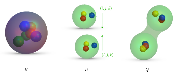
Figure 2: Graphical depiction of the three types of operators included in the numerical calculation. From left to right: hexaquark ($H$), dibaryon ($D$) and quasi-local ($Q$) operators. The relative momentum between the two nucleons in the dibaryon operators is labelled by $(i,j,k)$.

The one- and two-nucleon operators used in this study can be described conveniently using diquark fields

$$\mathcal{D}^{ab}_{\Gamma,F}(x)=\frac{1}{\sqrt{2}}q^{aT}(x)C\Gamma i\tau_{2}Fq^{b}(x)\ ,$$ (18)

where $q=(u,d)^{T}$ is an isodoublet quark field, $C=\gamma_{2}\gamma_{4}$ is the Euclidean charge conjugation matrix, $\tau_{2}=\left(\begin{smallmatrix}0&-i\\ i&0\end{smallmatrix}\right)$ is a Pauli matrix in isospin space, $F$ and $\Gamma$ are flavor and spin matrices, and $a$ and $b$ are color indices. Proton and neutron operators can be built from isosinglet diquarks

$$\mathcal{D}^{ab}_{\Gamma,\mathds{1}}(x)=\frac{1}{\sqrt{2}}\left[u^{aT}(x)C\Gamma d^{b}(x)-d^{aT}(x)C\Gamma u^{b}(x)\right]\ ,$$ (19)

where $\mathds{1}$ denotes the flavor identity matrix. In particular,

$$p_{\sigma}^{\Gamma}(x)=\epsilon_{abc}\mathcal{D}^{ab}_{\Gamma,\mathds{1}}(x)P_{\sigma}u^{c}(x)\ ,$$ (20)

$$n_{\sigma}^{\Gamma}(x)=\epsilon_{abc}\mathcal{D}^{ab}_{\Gamma,\mathds{1}}(x)P_{\sigma}d^{c}(x)\ ,$$ (21)

where $P_{\sigma}$ projects the quark spin to a specific row $\sigma\in\{0,\ldots,3\}$ of the spinor representation of $SO(4)$. In the Dirac basis, these projectors can be defined using parity projectors $P_{\pm}=(\mathds{1}\pm\gamma_{4})/2$ as

$$\begin{split}P_{\sigma}=\begin{cases}P_{+}\left(\mathds{1}-(-1)^{\sigma}i\gamma_{1}\gamma_{2}\right)/2,&\sigma\in\{0,1\}\ ,\\ P_{-}\left(\mathds{1}-(-1)^{\sigma}i\gamma_{1}\gamma_{2}\right)/2,&\sigma\in\{2,3\}\ .\end{cases}\end{split}$$ (22)

The isodoublet nucleon field $N=(p,n)^{T}$ is defined as

$$N_{\sigma}^{\Gamma}(x)=\epsilon_{abc}\mathcal{D}^{ab}_{\Gamma,\mathds{1}}(x)P_{\sigma}q^{c}(x)\ .$$ (23)

In addition to using the isosinglet diquark shown above, $I=1/2$ nucleon operators can be constructed using an isovector diquark $\mathcal{D}^{ab}_{\Gamma,\tau_{A}}$, where $A\in\{1,2,3\}$ is an adjoint isospin index. However, as shown in Ref. [96], quark antisymmetry can be used to relate the isovector diquark operators (which correspond to mixed-symmetric operators in Ref. [96]) to linear combinations of isoscalar diquark (mixed-antisymmetric) operators. A complete basis of local nucleon operators can therefore be obtained from $N_{\sigma}^{\Gamma}$ with all linearly independent choices of $\Gamma$ leading to nucleon quantum numbers, and is given by the three positive-parity and the three negative-parity operators presented in Ref. [96]. In the numerical calculations below, two positive-parity nucleon operators, given by

$$N_{\sigma}^{\gamma_{5}P_{+}}(x)=\epsilon_{abc}\mathcal{D}^{ab}_{\gamma_{5}P_{+},\mathds{1}}(x)P_{\sigma}q^{c}(x)\ ,$$ (24)

$$N_{\sigma}^{\gamma_{5}P_{-}}(x)=\epsilon_{abc}\mathcal{D}^{ab}_{\gamma_{5}P_{-},\mathds{1}}(x)P_{\sigma}q^{c}(x)\ ,$$ (25)

are included. The operator $N_{\sigma}^{\gamma_{5}P_{+}}$ involves only the Dirac basis upper components $\sigma\in\{0,1\}$ of the quark field and corresponds to the operator used in Ref. [56], while the operator $N_{\sigma}^{\gamma_{5}P_{-}}$ also involves the lower components $\sigma\in\{2,3\}$ in the diquark field (the nucleon spin is still restricted to $\sigma\in\{0,1\}$). Products of these operators will be used to build dibaryon operators as described below. Positive-parity dibaryon operators can also be constructed from products of two negative-parity nucleon operators such as

$$N_{\sigma}^{\mathds{1}}(x)=\epsilon_{abc}\mathcal{D}^{ab}_{\mathds{1},\mathds{1}}(x)P_{\sigma}q^{c}(x)\ .$$ (26)

The three linearly-independent nucleon operators that are not studied in this work are expected to overlap predominantly with excited states outside the low-energy region that is the focus of this work [97, 98, 99, 100].

III.2 Dibaryon Operators

Dibaryon operators are constructed from products of two-nucleon operators that are individually projected to definite momentum. Dibaryon operators with zero total three-momentum are defined by

$$D^{(2,I)\Gamma}_{\rho}(\vec{n},t)=\sum_{\vec{x}_{1},\vec{x}_{2}\in\Lambda_{\mathcal{S}}}e^{i{2\pi\over L}\vec{n}\cdot(\vec{x}_{1}-\vec{x}_{2})}\sum_{\sigma,\sigma^{\prime},u,u^{\prime}}v_{\rho}^{\sigma\sigma^{\prime}}P_{uu^{\prime}}^{(I)}N^{\Gamma}_{\sigma u}(\vec{x}_{1},t)N^{\Gamma}_{\sigma^{\prime}u^{\prime}}(\vec{x}_{2},t)\ ,$$ (27)

where $x=(\vec{x},t)$ are lattice coordinates whose components are integer multiple of the lattice spacing $a$, $L$ is the spatial extent of the lattice geometry, $\Lambda_{\mathcal{S}}$ is a sparse sublattice with $L/(a\mathcal{S})$ sites in each dimension that is introduced to make the volume sums computationally tractable as described in Refs. [101, 102, 56]. The index $\rho\in\{0,\ldots,3\}$ labels spin-singlet ($\rho=0$) and spin-triplet ($\rho\in\{1,2,3\}$) dibaryon operators, and $v_{\rho}^{\sigma\sigma^{\prime}}$ denotes Clebsch-Gordon coefficients (explicitly presented in Ref. [56]) projecting the product of two spin-1/2 operators into the particular dibaryon spin state. Quantum numbers, here baryon number $B=2$ and total isospin $I$, are denoted by superscripts in parantheses. Projection to operators with definite isospin is accomplished using $P^{(0)}=i\tau_{2}$ and $P^{(1)}=i\tau_{2}\tau_{3}$, where $I_{z}=0$ is chosen for simplicity and $u,u^{\prime}$ are flavor indices.

The set of dibaryon operators used here extends that of Ref. [56] by including dibaryon operators with $\Gamma=\gamma_{5}P_{-}$ and $\Gamma=\mathds{1}$ in addition to $\Gamma=\gamma_{5}P_{+}$. These dibaryon operators all have the same quantum numbers because products of two negative-parity nucleon operators ($\Gamma=\mathds{1}$) have positive parity. Analogous dibaryon operators can also be constructed in cases where the two nucleons each have different spin structures, as well as from other products of two-baryon operators, such as $\Delta\Delta$ and $N\Delta$, but the construction of this larger operator set is beyond the scope of this work.

For each $\Gamma$, operators with relative momenta $\vec{k}=(2\pi/L)\vec{n}$ are included with

$$\vec{n}\in\big{\{}(0,0,0),\ (0,0,1),\ (0,1,1),\ (1,1,1),\ (0,0,2),\ldots\big{\}}\ ,$$ (28)

where the ellipsis denotes momenta related to the ones that are shown by all possible cubic group transformations. Dibaryon operators that transform irreducibly under cubic transformations are obtained using appropriate averages of dibaryon operators with the same $|\vec{n}|$ but different $\vec{n}$. Defining the momentum orbit $K^{(s)}=\{\vec{n}\ \big{|}\ |\vec{n}|^{2}=s\}$, projection to a cubic irrep $\Gamma_{J}$ with a row labeled by $J_{z}$ is achieved by forming linear combinations

$$D^{(2,I,\Gamma_{J},J_{z})\Gamma}_{sm}(t)=\sum_{\vec{n}\in K^{(s)}}\sum_{\rho}G^{(\Gamma_{J},J_{z})}_{sm\vec{n}\rho}D^{(2,I)\Gamma}_{\rho}(\vec{n},t)\ ,$$ (29)

where $m\in\{1,2,3,\ldots,N_{s}^{\Gamma_{J}}\}$ indexes the operators arising for a given $s$, $\Gamma_{J}$, $J_{z}$, and $\Gamma$. For $I=1$ operators, $m\in\{1\}$ is trivial, while for $I=0$, spin-orbit coupling leads to non-trivial multiplicities $N_{s}^{\Gamma_{J}}$ for some $s$ and $\Gamma_{J}$ as discussed in Refs. [56, 103] and below. The change-of-basis coefficients $G^{(\Gamma_{J},J_{z})}_{sm\vec{n}\rho}$ are presented in Ref. [56] (see also Ref. [104]).

III.3 Quasi-local operators

Quasi-local operators are constructed using spatial wavefunctions that are chosen to mimic the form of the asymptotic wavefunction for the deuteron determined from nuclear EFTs and phenomenological models [58, 105, 106, 107], while having a factorizable form that enables efficient contraction calculations [56]. They are defined as

$$Q^{(2,I)\Gamma}_{\rho}(\kappa,t)=\sum_{\vec{x}_{1},\vec{x}_{2},R\in\Lambda_{\mathcal{S}}}e^{-\kappa|\vec{x}_{1}-\vec{R}|}e^{-\kappa|\vec{x}_{2}-\vec{R}|}\sum_{\sigma,\sigma^{\prime}}v_{\rho}^{\sigma\sigma^{\prime}}P_{uu^{\prime}}^{(I)}N^{\Gamma}_{\sigma u}(\vec{x}_{2},t)N^{\Gamma}_{\sigma^{\prime}u^{\prime}}(\vec{x}_{1},t)\ ,$$ (30)

where $\kappa$ is a parameter controlling the amount of correlation between the two nucleon positions, and $\vec{R}$ describes the center-of-mass of the two-nucleon system. The analog of Eq. (29) with $D^{(2,I)\Gamma}_{\rho}$ replaced by $Q^{(2,I)\Gamma}_{\rho}$ is used to project quasi-local operators onto rows of cubic irreps $\Gamma_{J}$ with definite $J_{z}$. As for the dibaryon operators, the set of quasi-local operators considered in Ref. [56] is extended here to quasi-local operators with $\Gamma\in\{\gamma_{5}P_{+},\gamma_{5}P_{-},\mathds{1}\}$.

III.4 Hexaquark operators

In this section, a complete basis of local (single-site or smeared) hexaquark operators which project onto two-nucleon states is constructed. The general hexaquark operator used to construct this basis is

$$\mathcal{H}_{K}^{(2,I,\Gamma_{J},J_{z})}(x)=\mathcal{H}^{C_{1}C_{2}C_{3}}_{G_{1},F_{1};G_{2},F_{2};G_{3},F_{3}}(x)=T^{C_{1}C_{2}C_{3}}_{abcdef}\mathcal{D}^{ab}_{G_{1},F_{1}}(x)\mathcal{D}^{cd}_{G_{2},F_{2}}(x)\mathcal{D}^{ef}_{G_{3},F_{3}}(x)\ ,$$ (31)

where $K=\{1,2,\dots\}$ corresponds to a particular spin-color-flavor structure. $T^{C_{1}C_{2}C_{3}}$ is a color tensor labeled by $C_{1}C_{2}C_{3}$ as described below, which projects the above operator to the color-singlet irrep, and diquarks $\mathcal{D}_{G_{i},F_{i}}$ with Dirac and flavor structures $G_{1},F_{1},\ldots,G_{3},F_{3}$ are defined in Eq. (18). In order to construct a complete basis of these operators, all possible color, spin and flavor labels must be enumerated. Only gauge invariant spin-singlet and spin-triplet operators with isospin zero and one are considered.

III.4.1 Color

Diquarks, being the product of two quarks, transform as $\mathbf{3}\otimes\mathbf{3}=\mathbf{6}\oplus\overline{\mathbf{3}}$ under $SU(3)_{c}$. Hexaquark operators formed from the product of three diquark operators therefore transform as

$$(\mathbf{3}\otimes\mathbf{3})\otimes(\mathbf{3}\otimes\mathbf{3})\otimes(\mathbf{3}\otimes\mathbf{3})=(\mathbf{6}\oplus\overline{\mathbf{3}})\otimes(\mathbf{6}\oplus\overline{\mathbf{3}})\otimes(\mathbf{6}\oplus\overline{\mathbf{3}})\ .$$ (32)

Not all of these terms contain a color-singlet in this irrep decomposition, but it appears once in each of the five products $\overline{\mathbf{3}}\otimes\overline{\mathbf{3}}\otimes\overline{\mathbf{3}},\ \overline{\mathbf{3}}\otimes\overline{\mathbf{3}}\otimes{\mathbf{6}},\ \overline{\mathbf{3}}\otimes{\mathbf{6}}\otimes\overline{\mathbf{3}},\ {\mathbf{6}}\otimes\overline{\mathbf{3}}\otimes\overline{\mathbf{3}}$, and ${\mathbf{6}}\otimes{\mathbf{6}}\otimes{\mathbf{6}}$. There are therefore five ways to combine the product of three diquarks into a color singlet. The corresponding color tensors are given by

$$T_{abcdef}^{AAA} =\epsilon_{abe}\epsilon_{cdf}-\epsilon_{abf}\epsilon_{cde}\ ,$$

$$T_{abcdef}^{AAS} =\epsilon_{abe}\epsilon_{cdf}+\epsilon_{abf}\epsilon_{cde}\ ,$$

$$T_{abcdef}^{ASA} =\epsilon_{abc}\epsilon_{efd}+\epsilon_{abd}\epsilon_{efc}\ ,$$ (33)

$$T_{abcdef}^{SAA} =\epsilon_{efa}\epsilon_{cdb}+\epsilon_{efb}\epsilon_{cda}\ ,$$

$$T_{abcdef}^{SSS} =\epsilon_{ace}\epsilon_{bdf}+\epsilon_{acf}\epsilon_{bde}+\epsilon_{bce}\epsilon_{adf}+\epsilon_{bcf}\epsilon_{ade}\ ,$$

where the labels $C_{1},C_{2},C_{3}\in\{A,S\}$ denote whether each tensor is antisymmetric or symmetric in each pair of indices $(a,b)$, $(c,d)$, and $(e,f)$, and hence is to be combined with a diquark in the $\overline{\mathbf{3}}$ or $\mathbf{6}$ representation for $A$ and $S$, respectively.

III.4.2 Spin

The operators introduced in Eq. (31) can be decomposed into (direct sums) of irreps of the relevant spatial symmetry group. In a continuous infinite volume, this group is $Spin(3)=SU(2)$ (i.e., the double cover of the $SO(3)$ spatial rotation group), under which two-nucleon states transform in either the spin-triplet or spin-singlet representations. On a periodic (hyper-)cubic lattice, the residual spatial symmetry is the double cover of the octahedral group, $O_{h}^{D}$. The isovector (spin-singlet) two-nucleon states transform in the $A_{1}^{+}$ irrep, while the isosinglet (spin-triplet) states transform in the $T_{1}^{+}$ irrep. In what follows, the continuum language of “spin-singlet” and “spin-triplet” will be used, as it unambiguoulsy specifies the internal spin degrees of freedom.

Recall from Eq. (18) above that each diquark contains a Dirac matrix of the form $CG_{i}$ where $C$ is the charge conjugation matrix. A possible basis for the matrices $G_{i}$ is given by

$$G_{i}\in\{P_{R},P_{L},P_{R}\gamma^{\mu},P_{L}\gamma^{\mu},\sigma^{\mu\nu}\}\ ,$$ (34)

where $P_{R/L}=\frac{1}{2}(\mathds{1}\pm\gamma_{5})$ and $\mu,\nu\in\{1,2,3,4\}$. In general, there are therefore $16^{3}=4096$ possible hexaquark spin structures. However, not all of these are independent. Fierz identities can be used to transform any product of two vector diquarks containing $\gamma^{\mu}$ or two tensor diquarks containing $\sigma^{\mu\nu}=\frac{i}{2}[\gamma^{\mu},\gamma^{\nu}]$ into a product of scalar diquarks [108]. Thus, when constructing the spin-singlet operator, it is sufficient to consider $G_{i}\in\{P_{R},P_{L}\}$. By a trivial change of basis, one can instead use the set $G_{i}\in\{\mathds{1},\gamma_{5}\}$ to construct a complete basis of $Spin(4)$-invariant hexaquark operators. For interpolating-operator construction, where the relevant symmetry group is $O_{h}^{D}$, additional insertions of $\gamma_{4}$ do not change diquark transformation properties (note that the $P_{\pm}$ projectors are used to isolate the upper/lower quark components). The Dirac matrices required for a complete basis of diquarks that are singlets under $O_{h}^{D}$ are, after a change of basis,

$$G_{i}\in\{\mathds{1},\gamma_{5},\gamma_{4},\gamma_{4}\gamma_{5}\}\ .$$ (35)

This leads to $4^{3}=64$ independent spin-singlet hexaquark operators.

Using the parity projection operators $P_{\pm}$, the 64 combinations can be split into a set of 32 positive-parity combinations and a set of 32 negative-parity combinations, with the parity of the hexaquark operator equal to the product of the parities of the diquarks. Positive-parity diquarks correspond to

$$G_{i}\in\{\gamma_{5}P_{+},\gamma_{5}P_{-}\}\ ,$$ (36)

while negative parity diquarks correspond to

$$G_{i}\in\{\mathds{1},\gamma_{4}\}\ .$$ (37)

This basis is convenient because it has definite symmetry properties for each diquark: diquarks with the Dirac matrix $C\gamma_{4}$ are symmetric under exchange of spin indices while diquarks with the $C$ and $C\gamma_{5}P_{\pm}$ Dirac matrices are antisymmetric. With this choice, operators that vanish due to quark antisymmetry can be easily identified.

For the spin-triplet hexaquark case, the only difference is that the construction must include one vector diquark whose Dirac structure includes one of the spin vector $S_{i}\equiv\tfrac{1}{2}\epsilon_{ijk}\gamma_{j}\gamma_{k}$ for $i\in\{1,2,3\}$. Since factors of $\gamma_{4}$ and $\gamma_{5}$ do not change $O_{h}^{D}$ transformation properties, these vector diquarks can involve four linearly independent Dirac matrices for a given spin index, $i$. To ensure definite exchange symmetry, the four independent structures can be taken to be $S_{i}$, $S_{i}\gamma_{4}$, and $S_{i}\gamma_{5}P_{\pm}$. Further appearances of spin-vector diquarks can be removed using Fierz relations as above. There are therefore 64 linearly independent spin structures relevant for spin-triplet hexaquark operators for each spin index, $i$,

$$G_{1}\in\{S_{i}\gamma_{5}P_{+},S_{i}\gamma_{5}P_{-},S_{i},S_{i}\gamma_{4}\}\ ,\hskip 10.0ptG_{2},G_{3}\in\{\gamma_{5}P_{+},\gamma_{5}P_{-},\mathds{1},\gamma_{4}\}\ ,$$ (38)

where the freedom to permute the diquarks to label the spin-vector diquark with $G_{1}$ has been used. As in the spin-singlet case, these operators can be split into sets of 32 operators with each parity. The positive-parity structures again correspond to operators with an odd number of structures involving $\gamma_{5}$.

III.4.3 Flavor

Assuming $SU(2)$ isospin symmetry is exact, products of two local nucleon operators form either an isovector spin-singlet state or an isoscalar spin-triplet state. Although hexaquark operators with other transformation properties, for example isosinglet spin-singlet, can be constructed, they will not mix with operators in these two channels.

Each diquark can be projected into isosinglet and isovector flavor irreps as

$$\begin{split}\mathcal{D}_{G,\mathds{1}}^{ab}(x)&=q^{aT}(x)CGi\tau_{2}q^{b}(x)\ ,\\ \mathcal{D}_{G,\tau_{A}}^{ab}(x)&=q^{aT}(x)CGi\tau_{2}\tau_{A}q^{b}(x)\ ,\end{split}$$ (39)

where $A\in\{1,2,3\}$. Five linearly independent operators with $I=0$ can be constructed from these building blocks,

$$\begin{split}&\mathcal{D}_{G_{1},\mathds{1}}^{ab}(x)\mathcal{D}_{G_{2},\mathds{1}}^{cd}(x)\mathcal{D}_{G_{3},\mathds{1}}^{ef}(x)\ ,\\ &\mathcal{D}_{G_{1},\tau_{A}}^{ab}(x)\mathcal{D}_{G_{2},\tau_{B}}^{cd}(x)\mathcal{D}_{G_{3},\mathds{1}}^{ef}(x)\delta_{AB}\ ,\\ &\mathcal{D}_{G_{1},\tau_{A}}^{ab}(x)\mathcal{D}_{G_{2},\mathds{1}}^{cd}(x)\mathcal{D}_{G_{3},\tau_{B}}^{ef}(x)\delta_{AB}\ ,\\ &\mathcal{D}_{G_{1},\mathds{1}}^{ab}(x)\mathcal{D}_{G_{2},\tau_{A}}^{cd}(x)\mathcal{D}_{G_{3},\tau_{B}}^{ef}(x)\delta_{AB}\ ,\\ &\mathcal{D}_{G_{1},\tau_{A}}^{ab}(x)\mathcal{D}_{G_{2},\tau_{B}}^{cd}(x)\mathcal{D}_{G_{3},\tau_{C}}^{ef}(x)\epsilon_{ABC}\ ,\end{split}$$ (40)

where $A,B,C\in\{1,2,3\}$. Note that the color and spin structures may differ on each diquark, making the second, third, and fourth combinations in Eq. (LABEL:eq:I0) distinct.

A total of nine linearly independent isospin tensor operators with $I=1$ can be constructed analogously,

$$\begin{split}&\mathcal{D}_{G_{1},\tau_{A}}^{ab}(x)\mathcal{D}_{G_{2},\mathds{1}}^{cd}(x)\mathcal{D}_{G_{3},\mathds{1}}^{ef}(x)\ ,\\ &\mathcal{D}_{G_{1},\mathds{1}}^{ab}(x)\mathcal{D}_{G_{2},\tau_{A}}^{cd}(x)\mathcal{D}_{G_{3},\mathds{1}}^{ef}(x)\ ,\\ &\mathcal{D}_{G_{1},\mathds{1}}^{ab}(x)\mathcal{D}_{G_{2},\mathds{1}}^{cd}(x)\mathcal{D}_{G_{3},\tau_{A}}^{ef}(x)\ ,\\ &\mathcal{D}_{G_{1},\tau_{B}}^{ab}(x)\mathcal{D}_{G_{2},\tau_{C}}^{cd}(x)\mathcal{D}_{G_{3},\mathds{1}}^{ef}(x)\epsilon_{ABC}\ ,\\ &\mathcal{D}_{G_{1},\tau_{B}}^{ab}(x)\mathcal{D}_{G_{2},\mathds{1}}^{cd}(x)\mathcal{D}_{G_{3},\tau_{C}}^{ef}(x)\epsilon_{ABC}\ ,\\ &\mathcal{D}_{G_{1},\mathds{1}}^{ab}(x)\mathcal{D}_{G_{2},\tau_{B}}^{cd}(x)\mathcal{D}_{G_{3},\tau_{C}}^{ef}(x)\epsilon_{ABC}\ ,\\ &\mathcal{D}_{G_{1},\tau_{A}}^{ab}(x)\mathcal{D}_{G_{2},\tau_{B}}^{cd}(x)\mathcal{D}_{G_{3},\tau_{C}}^{ef}(x)\delta_{BC}\ ,\\ &\mathcal{D}_{G_{1},\tau_{B}}^{ab}(x)\mathcal{D}_{G_{2},\tau_{A}}^{cd}(x)\mathcal{D}_{G_{3},\tau_{C}}^{ef}(x)\delta_{BC}\ ,\\ &\mathcal{D}_{G_{1},\tau_{B}}^{ab}(x)\mathcal{D}_{G_{2},\tau_{C}}^{cd}(x)\mathcal{D}_{G_{3},\tau_{A}}^{ef}(x)\delta_{BC}\ .\\ \end{split}$$ (41)

III.4.4 Gram-Schmidt Reduction and Hexaquark Basis

$K$

Color

Spin

Flavor

$K$

Color

Spin

Flavor

1

$A$

$A$

$A$

$\gamma_{4}$

$\gamma_{5}P_{+}$

$\mathds{1}$

$\tau$

$\mathds{1}$

$\mathds{1}$

9

$S$

$A$

$A$

$\gamma_{5}P_{-}$

$\gamma_{5}P_{+}$

$\gamma_{5}P_{+}$

$\tau$

$\mathds{1}$

$\mathds{1}$

2

$A$

$A$

$A$

$\gamma_{4}$

$\gamma_{5}P_{-}$

$\mathds{1}$

$\tau$

$\mathds{1}$

$\mathds{1}$

10

$S$

$A$

$A$

$\gamma_{5}P_{-}$

$\gamma_{5}P_{-}$

$\gamma_{5}P_{+}$

$\tau$

$\mathds{1}$

$\mathds{1}$

3

$S$

$A$

$A$

$\gamma_{5}P_{+}$

$\gamma_{5}P_{+}$

$\gamma_{5}P_{+}$

$\tau$

$\mathds{1}$

$\mathds{1}$

11

$S$

$A$

$A$

$\gamma_{5}P_{-}$

$\gamma_{5}P_{-}$

$\gamma_{5}P_{-}$

$\tau$

$\mathds{1}$

$\mathds{1}$

4

$S$

$A$

$A$

$\gamma_{5}P_{+}$

$\gamma_{5}P_{-}$

$\gamma_{5}P_{+}$

$\tau$

$\mathds{1}$

$\mathds{1}$

12

$S$

$A$

$A$

$\gamma_{5}P_{-}$

$\mathds{1}$

$\mathds{1}$

$\tau$

$\mathds{1}$

$\mathds{1}$

5

$S$

$A$

$A$

$\gamma_{5}P_{+}$

$\gamma_{5}P_{-}$

$\gamma_{5}P_{-}$

$\tau$

$\mathds{1}$

$\mathds{1}$

13

$S$

$A$

$A$

$\gamma_{5}P_{-}$

$\gamma_{4}$

$\gamma_{4}$

$\tau^{\prime}$

$\tau$

$\tau^{\prime}$

6

$S$

$A$

$A$

$\gamma_{5}P_{+}$

$\mathds{1}$

$\mathds{1}$

$\tau$

$\mathds{1}$

$\mathds{1}$

14

$S$

$A$

$A$

$\gamma_{5}P_{-}$

$\gamma_{4}$

$\gamma_{4}$

$\tau$

$\tau^{\prime}$

$\tau^{\prime}$

7

$S$

$A$

$A$

$\gamma_{5}P_{+}$

$\gamma_{4}$

$\gamma_{4}$

$\tau^{\prime}$

$\tau$

$\tau^{\prime}$

15

$S$

$S$

$S$

$\gamma_{5}P_{+}$

$\gamma_{5}P_{-}$

$\gamma_{5}P_{+}$

$\tau$

$\tau^{\prime}$

$\tau^{\prime}$

8

$S$

$A$

$A$

$\gamma_{5}P_{+}$

$\gamma_{4}$

$\gamma_{4}$

$\tau$

$\tau^{\prime}$

$\tau^{\prime}$

16

$S$

$S$

$S$

$\gamma_{5}P_{+}$

$\gamma_{5}P_{-}$

$\gamma_{5}P_{-}$

$\tau^{\prime}$

$\tau$

$\tau^{\prime}$

Table 1: A complete basis of hexaquark operators with $I=1$ and spin zero, $\mathcal{H}^{(2,1,A_{1}^{+},J_{z}=0)}_{K}(x)$, enumerated by $K\in\{1,\dots,16\}$. Note that all but $K=3$ constitute operators with hidden color. Each operator takes the form $\mathcal{H}^{C_{1}C_{2}C_{3}}_{G_{1},F_{1};G_{2},F_{2};G_{3},F_{3}}(x)$, where the color tensor labels $C_{i}$, Dirac matrices $G_{i}$, and flavor tensors $F_{i}$ appearing in each diquark as defined in the main text are indicated in the corresponding columns for each $K$. Here, $\tau$ always refers to an isovector diquark with a free isospin index, while $\tau^{\prime}$ pairs indicate isovector diquarks whose indices are contracted as $\tau^{\prime}_{B}\tau^{\prime}_{C}\delta_{BC}$.

$K$

Color

Spin

Flavor

$K$

Color

Spin

Flavor

1

$A$

$A$

$A$

$S_{i}\gamma_{5}P_{+}$

$\gamma_{4}$

$\mathds{1}$

$\tau$

$\tau$

$\mathds{1}$

9

$S$

$A$

$A$

$S_{i}\gamma_{5}P_{+}$

$\mathds{1}$

$\mathds{1}$

$\mathds{1}$

$\mathds{1}$

$\mathds{1}$

2

$A$

$A$

$A$

$S_{i}\gamma_{5}P_{-}$

$\gamma_{4}$

$\mathds{1}$

$\tau$

$\tau$

$\mathds{1}$

10

$S$

$A$

$A$

$S_{i}\gamma_{5}P_{-}$

$\gamma_{5}P_{-}$

$\gamma_{5}P_{+}$

$\mathds{1}$

$\mathds{1}$

$\mathds{1}$

3

$A$

$A$

$A$

$S_{i}$

$\gamma_{4}$

$\gamma_{5}P_{+}$

$\tau$

$\tau$

$\mathds{1}$

11

$S$

$A$

$A$

$S_{i}\gamma_{5}P_{-}$

$\gamma_{5}P_{-}$

$\gamma_{5}P_{-}$

$\mathds{1}$

$\mathds{1}$

$\mathds{1}$

4

$A$

$A$

$A$

$S_{i}\gamma_{4}$

$\gamma_{5}P_{+}$

$\mathds{1}$

$\mathds{1}$

$\mathds{1}$

$\mathds{1}$

12

$S$

$A$

$A$

$S_{i}\gamma_{5}P_{-}$

$\mathds{1}$

$\mathds{1}$

$\mathds{1}$

$\mathds{1}$

$\mathds{1}$

5

$A$

$A$

$A$

$S_{i}\gamma_{4}$

$\gamma_{5}P_{-}$

$\mathds{1}$

$\mathds{1}$

$\mathds{1}$

$\mathds{1}$

13

$S$

$S$

$S$

$S_{i}\gamma_{5}P_{+}$

$\gamma_{4}$

$\gamma_{4}$

$\mathds{1}$

$\mathds{1}$

$\mathds{1}$

6

$S$

$A$

$A$

$S_{i}\gamma_{5}P_{+}$

$\gamma_{5}P_{+}$

$\gamma_{5}P_{+}$

$\mathds{1}$

$\mathds{1}$

$\mathds{1}$

14

$S$

$S$

$S$

$S_{i}\gamma_{5}P_{-}$

$\gamma_{4}$

$\gamma_{4}$

$\mathds{1}$

$\mathds{1}$

$\mathds{1}$

7

$S$

$A$

$A$

$S_{i}\gamma_{5}P_{+}$

$\gamma_{5}P_{-}$

$\gamma_{5}P_{+}$

$\mathds{1}$

$\mathds{1}$

$\mathds{1}$

15

$S$

$S$

$S$

$S_{i}\gamma_{4}$

$\gamma_{4}$

$\gamma_{5}P_{+}$

$\tau$

$\mathds{1}$

$\tau$

8

$S$

$A$

$A$

$S_{i}\gamma_{5}P_{+}$

$\gamma_{5}P_{-}$

$\gamma_{5}P_{-}$

$\mathds{1}$

$\mathds{1}$

$\mathds{1}$

16

$A$

$A$

$S$

$S_{i}\gamma_{5}P_{+}$

$\gamma_{5}P_{-}$

$\gamma_{5}P_{-}$

$\tau$

$\mathds{1}$

$\tau$

Table 2: A complete basis of hexaquark operators with $I=0$ and spin one, $\mathcal{H}_{K}^{(2,0,T_{1}^{+},J_{z}=i)}(x)$, enumerated by $K\in\{1,\dots,16\}$. Note that all but $K=6$ constitute operators with hidden color. Color, spin, and flavor labels are as in Table 1. Here, the $\tau$ flavor structures correspond to contracted indices $\tau_{A}\tau_{B}\delta_{AB}$.

Spin-color-flavor tensor hexaquark operators are obtained by contracting the flavor tensor operators above with one of the five color tensors shown in Eq. (33) and choosing $G_{1}$, $G_{2}$, and $G_{3}$ to correspond to the choices of spin operators described in Sec. III.4.2. However, the resulting operators will not all be linearly independent because of quark antisymmetry. The reduction of this overcomplete set to complete bases of positive-parity spin-singlet hexaquark operators with $I=1$ and positive-parity spin-triplet hexaquark operators with $I=0$ is discussed in this section.

The five color tensors and 32 positive-parity spin-singlet tensors discussed above can be combined with the nine $I=1$ flavor tensors in $5\times 32\times 9=1440$ ways. Each of these spin-color-flavor tensor operators can be described as a contraction of six quark fields with a weight tensor that has six spin, color, and flavor indices. The resulting rank-18 weight tensors are sparse and can be represented efficiently as lists of the non-zero weights and their corresponding index values. To make the constraints from quark antisymmetry manifest, the quark fields appearing in every term with non-zero weights can be permuted into a fiducial flavor ordering, such as $uuuddd$ for the $I_{z}=0$ case, as described in Refs. [109, 56]. Many terms in the original weight tensor correspond to the same tensor structure after antisymmetrization and can be combined together to build a reduced rank-12 spin-color weight tensor corresponding to the fiducial ordering.

The reduced weight tensors associated with linearly independent spin-color-flavor tensor operators are not linearly independent if some operators are related by quark antisymmetry. An orthonormal basis of reduced-weight tensors is constructed using a Gram–Schmidt process; this basis is a complete basis of hexaquark operators without redundancies from quark antisymmetry or Fierz relations. The orthogonalization isolates 16 linearly independent operators from the full set of 1440 isovector spin-singlet hexaquark operators. Note that accounting for the quark antisymmetry of each individual diquark reduces the 1440 operators to 101; however, many of the remaining redundancies can be understood as arising from combined color-spin-flavor Fierz identities that complicate a group theoretic determination of the number of linearly independent operators [108, 110]. These 16 orthonormal operators $H_{i}^{(2,1,A_{1}^{+},J_{z})}(x)$ are linear combinations of the 16 spin-color-flavor tensor operators $\mathcal{H}^{(2,1,A_{1}^{+},J_{z})}_{K}(x)$ shown in Table 1,

$$H_{i}^{(2,1,A_{1}^{+},J_{z})}(x)=\sum_{K=1}^{i}w_{iK}^{(2,1,A_{1}^{+})}\sum_{\vec{x}}\mathcal{H}^{(2,1,A_{1}^{+},J_{z})}_{K}(x)\ .$$ (42)

Hexaquark operators with zero momentum are defined as $H_{i}^{(2,1,A_{1}^{+},J_{z})}(t)=\sum_{\vec{x}}H_{i}^{(2,1,A_{1}^{+},J_{z})}(\vec{x},t)$. It is noteworthy that normalized isovector hexaquark operators constructed from products of color-singlet upper-spin-component baryon operators of the forms $NN$, $N\Delta$, and $\Delta\Delta$ are all identical to the basis operator $H_{3}^{(2,1,A_{1}^{+},J_{z})}$. This can be explained by the fact that baryon-product operators of the forms $NN$, $N\Delta$, and $\Delta\Delta$ all include two diquarks that are antisymmetric in color and are comprised of only upper-spin-component quark fields — $H_{3}^{(2,1,A_{1}^{+},J_{z})}$ is the only basis operator, or linear combination of basis operators, meeting this description.

The same considerations apply to positive-parity spin-triplet hexaquarks with $I=0$, where five flavor tensors are available. In this case, a total of $5\times 32\times 5=800$ spin-color-flavor tensor operators can be constructed. As in the preceding spin-singlet case, reduced weights are constructed for each of these 800 operators. Finally, the Gram–Schmidt algorithm isolates 16 orthonormal spin-triplet hexaquark operators using linear combinations of the operators shown in Table 2. Normalized isosinglet hexaquark operators constructed from products of color-singlet upper-spin-component baryon operators of the forms $NN$ and $\Delta\Delta$ are both identical to the basis operator $H_{6}^{(2,0,T_{1}^{+},J_{z})}$, which can be explained analogously to the $I=1$ case.

IV Numerical Study with $m_{\pi}\approx 806~{}$\mathrm{M}\mathrm{e}\mathrm{V}$$

This section presents a variational study of the spectrum of two-nucleon systems for $N_{f}=3$ degenerate quarks with a common mass corresponding to a pion mass of $m_{\pi}\approx 806~{}$\mathrm{M}\mathrm{e}\mathrm{V}$$. This calculation uses gauge fields also employed in previous studies of two-nucleon spectroscopy in Refs. [46, 47, 54, 48, 56] which were generated using the tadpole-improved Lüscher-Weisz gauge field action [111] with a single level of stout smearing [112] and the Wilson-clover fermion action [113] with a tadpole-improved tree-level clover coefficient $c_{SW}=1.2493$ [114]. Relevant details are presented in Table. 3.

Quark propagators computed for all source points in a $6^{3}$ sparse sub-lattice of the $(L/a)^{3}=24^{3}$ spatial volume at a fixed time are used to construct sparsened quark propagators [101] with sparseining factor $\mathcal{S}=4$. The quark sources employ gauge-invariant Gaussian smearing [115, 116] with a Chroma smearing parameter 2.1, which corresponds to a Gaussian smearing width of $\approx 0.18$ fm. Interpolating operators constructed from these quark propagators are therefore identical to the “thin”-smearing operators described in Ref. [56] except that an ensemble with larger $L$ is used in that work. Variational bounds on the one- and two-nucleon systems are obtained by performing multi-exponential fits to the principal correlation functions determined from the GEVP, following the algorithm described previously in Refs. [50, 56] augmented by the algorithm for choosing reference times $t_{0}$ and $t_{\rm ref}$ discussed in Appendix A.

$(L/a)^{3}\times(T/a)$	$\beta$	$am_{q}$	$a$ [$\mathrm{f}\mathrm{m}$]	$L$ [$\mathrm{f}\mathrm{m}$]	$T$ [$\mathrm{f}\mathrm{m}$]	$m_{\pi}L$	$m_{\pi}T$	$N_{\text{cfg}}$	$N_{\text{src}}$
$24^{3}\times 48$	6.1	-0.2450	0.1453(16)	3.4	6.7	14.3	28.5	469	216

Table 3: Details of the ensemble of gauge field configurations used for the numerical calculations. $L$ and $T$ are the spatial and temporal extents of the lattice, $\beta=6/g^{2}$ is the inverse bare coupling, $m_{q}$ is the bare quark mass, $a$ is the lattice spacing, $N_{\text{cfg}}$ is the total number of gauge field configurations used, and $N_{\text{src}}$ is the number of source locations employed on each configuration.

IV.1 Interpolating-operator sets

A range of different variational operator sets are considered. Sets are chosen to study the operator dependence of variational bounds on the energy eigenvalues. Understanding this variation is critical because a complete basis of operators for the full Hilbert space of QCD remains intractable.

Shorthand notation is useful for discussing interpolating-operator sets and variational bounds. The positive- and negative-parity single-nucleon channels have quantum numbers $Q=(B,I,\Gamma_{J})$ that will be denoted

$$N^{+} \equiv(1,\tfrac{1}{2},G_{1}^{+})\ ,$$ (43)

$$N^{-} \equiv(1,\tfrac{1}{2},G_{1}^{-})\ .$$ (44)

The energy spectrum is independent of $J_{z}$; numerical calculations average $N^{+}$ and $N^{-}$ correlation functions over $J_{z}\in\{1,2\}$. The quantum numbers $Q=(B,I,\Gamma_{J})$ for the two-baryon systems are

$$nn \equiv(2,1,A_{1}^{+})\ ,$$ (45)

$$d \equiv(2,0,T_{1}^{+})\ .$$ (46)

Note that $nn$ is used to label the “dineutron” $I=1$ spectrum, which is independent of $I_{z}$; numerical calculations are explicitly performed using $I_{z}=0$. Similarly, the label $d$ is used to denote the isoscalar spin-triplet spectrum, which is independent of $J_{z}$; numerical calculations average correlation functions over $J_{z}\in\{1,2,3\}$. Notation for energy gaps in these channels is summarized in Table 4.

The sets of operators that are studied in this work can be divided broadly into three main categories:

1. Dibaryon operator sets include a range of different dibaryon operators, including those with lower-spin components and negative parity nucleon operators. Dibaryon operator sets are denoted $\mathbb{S}_{N_{D}D}^{Q}$, where $Q\in\{nn,d\}$ denotes the quantum numbers of the system and $N_{D}$ is the number of dibaryon operators in the set.

2. Hexaquark operator sets include a variety of hexaquark operators from Sec. III.4. Hexaquark operator sets are denoted $\mathbb{S}_{N_{H}H}^{Q}$, with $Q$ as above and $N_{H}$ the number of hexaquark operators that are included.

3. Dibaryon and hexaquark operator sets combine operators from the previous two sets to examine the combined effect of both types of operators. Combined operator sets are denoted $\mathbb{S}_{N_{D}D}^{Q}\cup\mathbb{S}_{N_{H}H}^{Q}$. The integers $N_{D}$ and $N_{H}$ correspond to the number of dibaryon and hexaquark operators, respectively. Thus, a total of $N_{D}$ + $N_{H}$ operators appear in the combined set.

Quantity	Description
$M_{N}\equiv E_{0}^{N^{+}}$	Nucleon mass
$\delta E^{N^{+}}\equiv E_{1}^{N^{+}}-M_{N}$	Energy gap in channel $N_{+}$
$\delta E^{N^{-}}\equiv E_{0}^{N^{-}}-M_{N}$	Energy gap in channel $N_{-}$ between lowest-energy negative-parity state and positive-parity ground state
$\Delta E_{\mathsf{n}}^{Q}\equiv E_{\mathsf{n}}^{Q}-2M_{N}$	$\mathsf{n}$th energy gap from two-nucleon threshold in channel $Q$, computed using fit results for each energy level
$\Delta E_{\mathsf{n}}^{Q}(t)\equiv E_{\mathsf{n}}^{Q}(t)-2E_{0}^{N^{+}}(t)$	Time-dependent $\mathsf{n}$th energy gap from two-nucleon threshold in channel $Q$, computed using the effective energies defined in Eq. 16
$\Delta_{\text{cut}}\equiv 2\sqrt{M_{N}^{2}+5\left(\frac{2\pi}{L}\right)^{2}}-2M_{N}$	Energy gap from two-nucleon threshold to the first non-interacting energy level with larger momentum than the operators used here

Table 4: Summary of spectral quantities used to characterize the low-energy one- and two-nucleon spectra. Single-nucleon splittings are denoted by $\delta$, while two-nucleon splittings use $\Delta$.

Sets of dibaryon operators constructed using upper-spin-component diquarks are defined by

$$\begin{split}\mathbb{S}_{5D}^{nn}\equiv\bigg{\{}D^{nn\Gamma}_{sm}(t)\,\bigg{|}\,s\in\{0,1,2,3,4\},m\in\{1,\ldots,N_{s}^{A_{1}^{+}}\},\ \Gamma\in\{\gamma_{5}P_{+}\}\bigg{\}}\ ,\\ \mathbb{S}_{10D}^{d}\equiv\bigg{\{}D^{d\Gamma}_{sm}(t)\,\bigg{|}\,s\in\{0,1,2,3,4\},m\in\{1,\ldots,N_{s}^{T_{1}^{+}}\},\ \Gamma\in\{\gamma_{5}P_{+}\}\bigg{\}}\ .\end{split}$$ (47)

On the right-hand side, $s=|\vec{n}|^{2}$ is the magnitude of the plane-wave momentum appearing in Eq. 27 and $m$ indexes the multiplicity of each shell. These sets are analogous to the interpolating-operator set denoted $\mathbb{S}_{0}$ in Ref. [56], except that operators with a second Gaussian quark field smearing were also included in Ref. [56].

Sets of dibaryon operators involving products of two negative-parity nucleons and involving nucleon operators built from lower-spin-component diquarks are defined by

$$\begin{split}\mathbb{S}_{10D}^{nn}\equiv&\bigg{\{}D^{nn\Gamma}_{sm}(t)\,\bigg{|}\,s\in\{0,1,2,3,4\},m\in\{1,\ldots,N_{s}^{A_{1}^{+}}\},\ \Gamma\in\{\gamma_{5}P_{+},\mathds{1}\}\bigg{\}}\ ,\\ \mathbb{S}_{15D}^{nn}\equiv&\bigg{\{}D^{nn\Gamma}_{sm}(t)\,\bigg{|}\,s\in\{0,1,2,3,4\},m\in\{1,\ldots,N_{s}^{A_{1}^{+}}\},\ \Gamma\in\{\gamma_{5}P_{+},\mathds{1},\gamma_{5}P_{-}\}\bigg{\}}\ ,\\ \mathbb{S}_{20D}^{d}\equiv&\bigg{\{}D^{d\Gamma}_{sm}(t)\,\bigg{|}\,s\in\{0,1,2,3,4\},m\in\{1,\ldots,N_{s}^{T_{1}^{+}}\},\ \Gamma\in\{\gamma_{5}P_{+},\mathds{1}\}\bigg{\}}\ ,\\ \mathbb{S}_{30D}^{d}\equiv&\bigg{\{}D^{d\Gamma}_{sm}(t)\,\bigg{|}\,s\in\{0,1,2,3,4\},m\in\{1,\ldots,N_{s}^{T_{1}^{+}}\},\ \Gamma\in\{\gamma_{5}P_{+},\mathds{1},\gamma_{5}P_{-}\}\bigg{\}}\ .\end{split}$$ (48)

The meanings of $s$, and $m$ are the same as in the preceding equation.

Compared to dibaryon operators, spatially localized hexaquark operators might be expected to have larger overlap with compact bound states and smaller overlap with scattering states. Sets containing one, two, and sixteen hexaquark operators are considered in order to study the variational bounds from hexaquark operators alone. For the dineutron, these sets are defined as

$$\begin{split}\mathbb{S}_{1H}^{nn}\equiv&\bigg{\{}H_{i}^{nn}(t)\,\bigg{|}\,i\in\{3\}\bigg{\}}\ ,\\ \mathbb{S}_{2H}^{nn}\equiv&\bigg{\{}H_{i}^{nn}(t)\,\bigg{|}\,i\in\{3,4\}\bigg{\}}\ ,\\ \mathbb{S}_{16H}^{nn}\equiv&\bigg{\{}H_{i}^{nn}(t)\,\bigg{|}\,i\in\{1,2,\dots,16\}\bigg{\}}\ .\end{split}$$ (49)

The dineutron operators $H^{nn}_{i}(t)$ appearing on the right-hand side are defined Eq. 42 as orthogonal linear combinations of the basic hexaquark operators in Table 1. The operator $H_{3}^{nn}(t)$ appearing in all three sets is identical, apart from an irrelevant constant, to the product of color-singlet nucleon operators centered at the same point that was studied in Ref. [56]. Explicitly, the two operators appearing in $\mathbb{S}_{2H}^{nn}$ are

$$\begin{split}H_{3}^{nn}(x)&=\mathcal{H}_{3}^{nn}(x)\ ,\\ H_{4}^{nn}(x)&=\mathcal{H}_{4}^{nn}(x)-\frac{1}{3}\mathcal{H}_{1}^{nn}(x)\ .\end{split}$$ (50)

For the deuteron, the corresponding operator sets are defined as

$$\begin{split}\mathbb{S}_{1H}^{d}\equiv&\bigg{\{}H_{i}^{d}(t)\,\bigg{|}\,i\in\{6\}\bigg{\}}\ ,\\ \mathbb{S}_{2H}^{d}\equiv&\bigg{\{}H_{i}^{d}(t)\,\bigg{|}\,i\in\{6,7\}\bigg{\}}\ ,\\ \mathbb{S}_{16H}^{d}\equiv&\bigg{\{}H_{i}^{d}(t)\,\bigg{|}\,i\in\{1,2,\dots,16\}\bigg{\}}\ ,\end{split}$$ (51)

where

$$\begin{split}H_{6}^{d}(x)&=\mathcal{H}_{6}^{d}(x)\ ,\\ H_{7}^{d}(x)&=\mathcal{H}_{7}^{d}(x)+\frac{3}{14}\mathcal{H}_{4}^{d}(x)-\frac{11}{42}\mathcal{H}_{3}^{d}(x)-\frac{2}{21}\mathcal{H}_{1}^{d}(x)\ .\end{split}$$ (52)

As in the dineutron channel, the operator $H_{6}^{d}(t)$ appearing in all three sets is identical to a product of color-singlet nucleon operators. The second operators included in $\mathbb{S}_{2H}^{Q}$ for each channel are chosen because of their relatively large overlaps with low-energy states in the numerical results below.

Four additional interpolating-operator sets are chosen for each channel to study the combined effects of including both dibaryon and hexaquark operators,

$$\begin{split}&\mathbb{S}_{5D}^{nn}\cup\mathbb{S}_{1H}^{nn}\ ,\quad\mathbb{S}_{5D}^{nn}\cup\mathbb{S}_{2H}^{nn}\ ,\quad\mathbb{S}_{5D}^{nn}\cup\mathbb{S}_{16H}^{nn}\ ,\quad\mathbb{S}_{15D}^{nn}\cup\mathbb{S}_{16H}^{nn}\ ,\\ &\mathbb{S}_{10D}^{d}\cup\mathbb{S}_{1H}^{d}\ ,\quad\mathbb{S}_{10D}^{d}\cup\mathbb{S}_{2H}^{d}\ ,\quad\mathbb{S}_{10D}^{d}\cup\mathbb{S}_{16H}^{d}\ ,\quad\mathbb{S}_{30D}^{d}\cup\mathbb{S}_{16H}^{d}\ .\end{split}$$ (53)

It is possible to define additional sets including quasi-local operators. In practice, such sets give results for the low-energy spectra which are consistent with one or more of the operator sets reported here, albeit with larger uncertainties. Results for operator sets including quasi-local operators are therefore not presented below.

Dibaryon operators with all three choices of $\Gamma\in\{\mathds{1},\gamma_{5}P_{+},\gamma_{5}P_{-}\}$ are also computed for cubic irreps that are associated with $D$-wave phase shifts in infinite volume. For the $I=1$ case, such dibaryon operators are constructed for $\Gamma_{J}=E^{+}$ with $s\in\{1,2,4\}$ and for $\Gamma_{J}=T_{2}^{+}$ with $s\in\{2,3\}$. For the $I=0$ case, dibaryon operators are constructed for $\Gamma_{J}=A_{2}^{+}$ with $s\in\{2,3\}$, for $\Gamma_{J}=E^{+}$ with $s\in\{2,3\}$, and for $\Gamma_{J}=T_{2}^{+}$ with $s\in\{1,2,3,4\}$. Although there are no hexaquarks built from products of color-singlet nucleons that transform in these representations, hexaquarks built from $N\Delta$ and $\Delta\Delta$ operators, as well as hidden-color operators, can be constructed that transform in the same representations. The inclusion of such operators is left to future work.

IV.2 The Single-Nucleon Channel

The positive-parity single-nucleon channel can be studied using the interpolating-operator set $\mathbb{S}^{N^{+}}=\{N^{\Gamma}\,|\,\Gamma\in\gamma_{5}P_{\pm}\}$, with the quantum numbers $N^{+}$ defined in Eq. 43. Applying the algorithm for selecting $t_{0}$ and $t_{\text{ref}}$ discussed in Appendix A leads to $t_{0}=7$ and $t_{\text{ref}}=11$. The effective masses and fit results using the multi-state fitting algorithm detailed in Refs. [50, 56] are shown in Fig. 3. The variational bound on the nucleon mass obtained from fits to the $\mathsf{n}=0$ principal correlation function is

$$aM_{N}\equiv aE_{0}^{N^{+}}=1.2036(15)\ ,$$ (54)

which is consistent with previous analyses of this ensemble [46, 48]. The variational bound on the first excited state in this channel obtained from analogous fits to the $\mathsf{n}=1$ principal correlation function is

$$aE_{1}^{N^{+}}=1.928(47)\ .$$ (55)

This bound is weaker than the corresponding bound $aE_{1}^{N^{+}}=1.770(14)$ obtained using a set of two interpolating operators with different Gaussian smearing widths on a larger spatial volume in Ref. [56]. The presence of significant excited-state contamination is unsurprising, since it is the second eigenvalue from a $2\times 2$ matrix of correlation functions, and further since Fig. 3 shows there may still be significant time-dependence in the effective energy at imaginary times where the signal is lost to noise. The insets in Fig. 3 show the overlaps with the ground and first excited states with upper- and lower-component operators. The ground state has similar overlaps, 0.548(1) and 0.452(1), with the respective upper- and lower-component operators. The first excited state overlaps dominantly with the lower-spin-component operator.

The negative-parity single-nucleon sector is orthogonal and is studied using the interpolating-operator set with a single operator $\mathbb{S}^{N^{-}}=\{N^{\mathds{1}}\}$. The resulting diagonal correlation function is positive definite and provides a variational bound on the lowest-energy negative-parity state,

$$aE_{0}^{N^{-}}=1.6357(76)\ ,$$ (56)

as shown in Fig. 4.

Constraints on the single-nucleon energy gaps defined in Table 4, $a\delta E^{N^{+}}=0.73(5)$ and $a\delta E^{N^{-}}=0.43(1)$, can inform interpretations of the two-nucleon energy spectrum. In particular, two-nucleon states with energies near $a\delta E^{N^{+}}$ might be associated with $N^{+}(N^{+})^{*}$ scattering states. Since positive-parity two-nucleon states include either zero or two negative-parity nucleon operators, states with energies near $a\delta E^{N^{-}}$ are not expected to appear in the positive-parity two-nucleon sector, while states with energies near $2a\delta E^{N^{-}}$ might be associated with $N^{-}N^{-}$ scattering states.

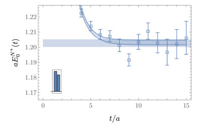
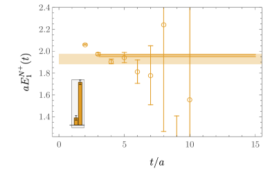
Figure 3: The positive parity single-nucleon channel is studied using the variational method utilizing a set of two operators constructed from the upper- and lower-spin components. The relative weights of the upper and lower spin components are shown as the left and right columns in the histogram (inset). The lower variational bound constrains the nucleon mass in lattice units. Lightly shaded colored bands show the total statistical plus fitting systematic uncertainties added in quadrature while the outlined regions show the statistical uncertainty of the highest-weight fit. Note that for the $\mathsf{n}=1$ case, fit results provide a variational bound even though there may still be significant curvature in the effective energy for all $t$ where signals can be resolved from noise.

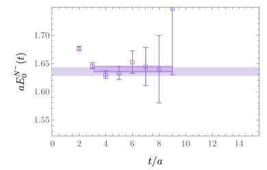
Figure 4: The negative parity nucleon channel is studied using the single negative parity nucleon operator defined in Eq. (26).

IV.3 Two-Nucleon Spectroscopy

Since one- and two-nucleon correlation functions are computed on the same gauge-field configurations, statistical fluctuations are strongly correlated between them. Consequently, correlated differences often lead to reduced statistical uncertainties. In particular, correlated energy differences (e.g., from the differences between separate fits to one- and two-nucleon correlation functions) are more precisely determined than total energies. Results are presented below for the effective energy gap $a\Delta E_{\mathsf{n}}^{Q}(t)$ defined in Table 4, where $t_{0}$ and $t_{\text{ref}}$ have been chosen as detailed in Appendix A. Critically, variational bounds are obtained from correlated fits to the one- and two-nucleon principal correlation functions individually and not to $a\Delta E_{\mathsf{n}}^{(2,I,\Gamma_{J})}(t)$, which is not a convex sum of exponentials. Individual variational bounds from fits to one- and two-nucleon correlation functions also furnish results for the energy gap $a\Delta E_{\mathsf{n}}^{Q}$ defined in Table 4. Energy gaps $a\Delta E_{\mathsf{n}}^{Q}$ are computed using the bootstrap methods described in Ref. [56]. Appendix B collects the strongest variational bounds on $a\Delta E_{\mathsf{n}}^{Q}$ for all $Q=(2,I,\Gamma_{J})$ studied in the present work.

Before presenting results, it is useful to consider where the near-threshold variational bounds would be expected to appear in the absence of hadronic interactions. In the present work, dibaryon operators are projected to all plane-wave momenta with $|\vec{n}|^{2}<5$. Therefore it may be expected that these operators will overlap predominately with finite-volume scattering states with energy gaps

$$a\Delta E\lesssim a\Delta_{\text{cut}}\equiv 2\sqrt{(aM_{N})^{2}+5(2\pi a/L)^{2}}-2aM_{N}=0.27\ ,$$ (57)

where $aM_{N}$ is given in Eq. 54 and $\Delta_{\text{cut}}$ is the non-interacting energy difference corresponding to $|\vec{n}|^{2}=5$; see Table 4. This energy region aligns with the energy region $a\Delta E\lesssim 0.24$ studied using plane-wave momentum-projected operators with $|\vec{n}|^{2}<8$ on an ensemble with larger volume in Ref. [56]. Additional multi-hadron states that have small overlap with these dibaryon operators may be present at similar or somewhat lower energies than $\Delta_{\text{cut}}$, in particular $N\Delta$ states with $I=1$ and $\Delta\Delta$ states with $I\in\{0,1\}$. Using the mass of the $\Delta$ baryon (stable at these values of the quark masses) computed using this gauge-field ensemble in Ref. [117], $aM_{\Delta}=1.3321(21)$, the threshold for $S$-wave $\Delta\Delta$ states with $nn$ or $d$ quantum numbers is $a\Delta E^{\Delta\Delta}\equiv 2aM_{\Delta}-2aM_{N}=0.26$. The corresponding threshold for $D$-wave $N\Delta$ states with $nn$ quantum numbers is $a\Delta E^{N\Delta}\equiv\sqrt{(aM_{\Delta})^{2}+(2\pi a/L)^{2}}+\sqrt{(aM_{N})^{2}+(2\pi a/L)^{2}}-2aM_{N}=0.18$. Variational bounds above these non-interacting thresholds still provide valid bounds satisfying the interlacing theorem. However, such bounds seem very unlikely to have saturated due to small, though exponentially growing in $t$, contributions to the associated principal correlation functions from $N\Delta$ and $\Delta\Delta$ states. These thresholds will be indicated in the numerical results below.

IV.3.1 The Dineutron Channel

The energy spectrum for two-nucleon systems with $I=1$ is independent of $I_{z}$ in the isospin-symmetric limit considered here. Therefore the results for $nn$, $pp$, and spin-singlet $pn$ systems are equivalent. This channel will be referred to as the dineutron channel in order to distinguish it from the $I=0$, spin-triplet deuteron channel. The most important contributions to the near-threshold scattering amplitude come from the $\ell=0$ partial-wave, as higher partial-waves are kinematically suppressed. In this section, results are given for the $A_{1}^{+}$ irrep, which corresponds to states with orbital angular momentum, $\ell\in\{0,4,6,\ldots\}$ in the continuum and infinite-volume limit [118, 119, 105, 103]. Effective masses from four representative operator sets are shown in Fig. 5. Variational bounds from each of the operator sets defined in the previous section are presented in Fig. 6.

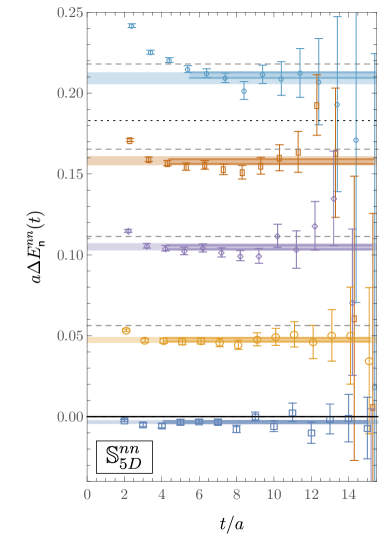
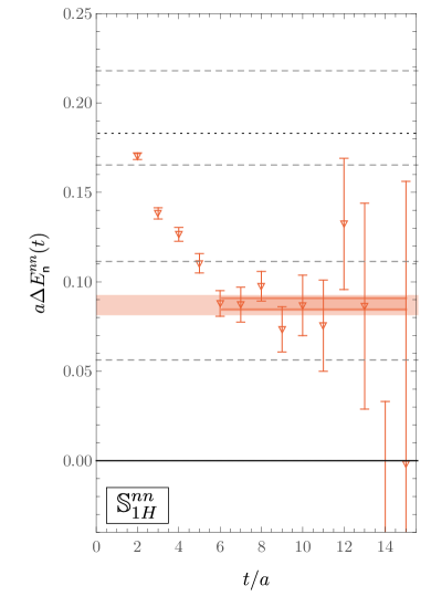
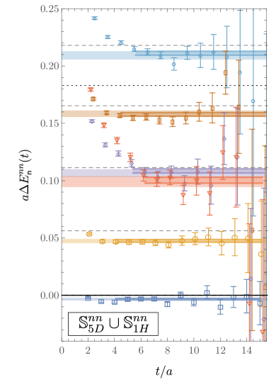
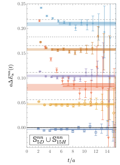
Figure 5: Effective mass functions and spectral bounds for operator sets $\mathbb{S}_{5D}^{{nn}}$ (upper left), $\mathbb{S}_{1H}^{{nn}}$ (upper right), $\mathbb{S}_{5D}^{{nn}}\cup\mathbb{S}_{1H}^{{nn}}$ (lower left), and $\mathbb{S}_{5D}^{{nn}}\cup\mathbb{S}_{16H}^{{nn}}$ (lower right) for the dineutron, $(B,I,\Gamma_{J})=(2,1,A_{1}^{+})$. Non-interacting $NN$ and $N\Delta$ energy levels are represented as dashed and dotted horizontal lines, respectively.

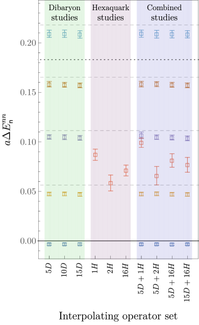
Figure 6: Summary of variational bounds on the low-lying dineutron $(B,I,\Gamma_{J})=(2,1,A_{1}^{+})$ spectrum obtained from all operator sets considered in this work. Non-interacting $NN$ and $N\Delta$ energy levels are represented as dashed and dotted horizontal lines, respectively.

In each of the dibaryon operator sets $\mathbb{S}_{5D}^{nn}$, $\mathbb{S}_{10D}^{nn}$ and $\mathbb{S}_{15D}^{nn}$, denoted “Dibaryon Studies” in Fig. 6, there exists a variational bound which lies just below each non-interacting two-nucleon energy level. This placement suggests that these bounds may be associated with attractive finite-volume $NN$ scattering states. Results for the sets $\mathbb{S}_{10D}^{nn}$ and $\mathbb{S}_{15D}^{nn}$ are consistent with those from the $\mathbb{S}_{5D}^{nn}$ set for all variational bounds below $\Delta_{\text{cut}}$. Differences between the variational bounds from each interpolating-operator set are smaller than the statistical uncertainties. The lowest energy bound is just below the two-nucleon threshold. This bound is higher than the previous estimates of the ground state energy on this ensemble using asymmetric source and sink interpolating operators and is therefore consistent in the sense of a variational bound.

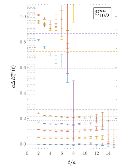
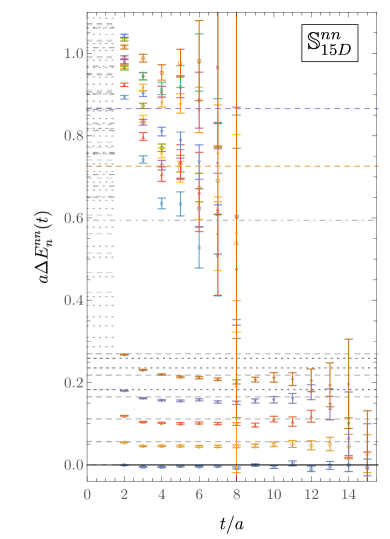
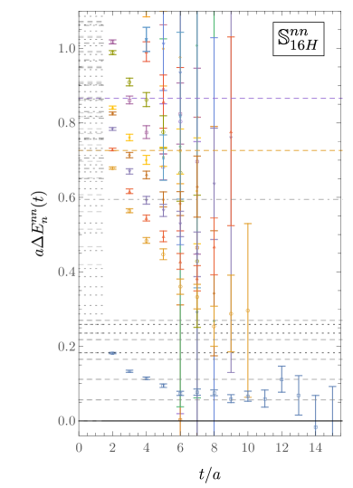
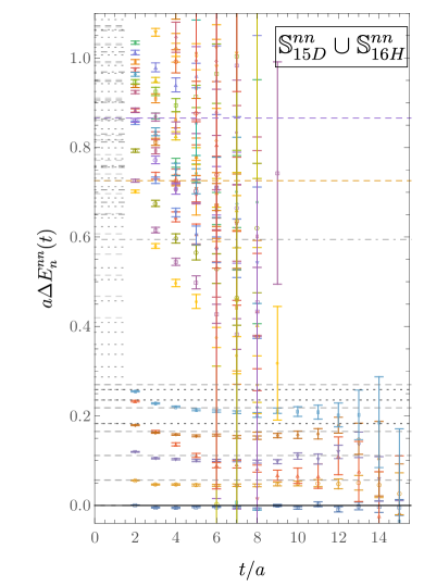
Figure 7: The effective mass spectra showing all of the variational bounds obtained with the interpolating-operator sets indicated. Non-interacting energy levels are represented as follows: dashed gray lines for $NN$; dotted black lines for $N\Delta$ and $\Delta\Delta$; and dot-dashed gray lines for $NN\pi$. Lines for non-interacting energy levels above $a\Delta_{\text{cut}}$ are cut off for visual clarity. Thresholds related to single-nucleon excitations are also indicated: dashed orange line for $a\delta E^{N^{+}}$ and dashed purple line for $a\delta E^{N^{+}}$.

Additional bounds not present for $\mathbb{S}_{5D}^{nn}$ appear in results for $\mathbb{S}_{10D}^{nn}$ and $\mathbb{S}_{15D}^{nn}$ at higher energies, as shown in Fig. 7. For $\mathbb{S}_{10D}^{nn}$, which contains dibaryon operators constructed from products of negative-parity nucleon operators, all but one of the additional bounds are above the threshold $2a\delta E^{N^{-}}\approx 0.87$ For $\mathbb{S}_{15D}^{nn}$, several additional bounds appear around $a\delta E^{N^{+}}\approx 0.74$. This suggests that these operators predominantly overlap with $N^{-}N^{-}$ and $N^{+}(N^{+})^{*}$ scattering states, although the presence of one bound below $a\delta E^{N^{+}}$ shows that they do not overlap exclusively with such states.

The sets $\mathbb{S}_{1H}^{nn}$, $\mathbb{S}_{2H}^{nn}$ and $\mathbb{S}_{16H}^{nn}$ furnish variational bounds for energy eigenstates obtained from operator sets which contain only hexaquark operators. While these sets may seem unnatural since they lack the dibaryon operators, which have been observed to have significant overlap with low-energy two-nucleon-like states, the interlacing theorem implies that $\mathbb{S}_{16H}$ nevertheless provides valid variational bounds on the lowest sixteen energy eigenvalues in the theory. The variational bounds determined from these interpolating-operator sets are shown in Figs. 5 - 7. For each hexaquark operator set described here, it is possible to observe a plateau at late Euclidean times in the $\mathsf{n}=0$ principal correlator. In each operator set, the variational bound on the lowest energy is $a\Delta E_{0}^{d}\approx 0.07$ above the two-nucleon threshold. For each of these hexaquark-only operator sets, the other variational bounds are above $\Delta_{\text{cut}}$ and do not exhibit clear plateaus, as shown in Fig. 7.

For the operator sets which include the upper-spin-component positive-parity dibaryon operators and either one, two, or sixteen hexaquark operators ($\mathbb{S}_{5D}^{nn}\cup\mathbb{S}_{1H}^{nn}$, $\mathbb{S}_{5D}^{nn}\cup\mathbb{S}_{2H}^{nn}$ and $\mathbb{S}_{5D}^{nn}\cup\mathbb{S}_{16H}^{nn}$) and for the operator set which includes all dibaryon and hexaquark operators ($\mathbb{S}_{15D}^{nn}\cup\mathbb{S}_{16H}^{nn}$), the resulting low-energy spectrum appears to be approximately the union of spectra for the dibaryon-only and hexaquark-only operator sets. Based on the numerically-determined variational bounds obtained from these operator sets, there exists an additional energy eigenvalue below $a\Delta E^{nn}\lesssim 0.1$ beyond those expected in a non-interacting two-nucleon system.

This additional level is constrained by the variational bound $a\Delta E_{2}^{nn}=0.077(7)$ from $\mathbb{S}_{15D}^{nn}\cup\mathbb{S}_{16H}^{nn}$ to be significantly below the non-interacting $N\Delta$ threshold $a\Delta E^{N\Delta}=0.183(6)$. The energy of an attractive but unbound $N\Delta$ system can be shifted from this value by roughly $-0.005$ [58, 105, 120, 121] before it becomes a bound state so this constraint precludes interpretation of the additional state as an $N\Delta$ scattering state. Interpretation of the additional state as a $NN$ resonance (e.g., a $N\Delta$ bound state) cannot be excluded.

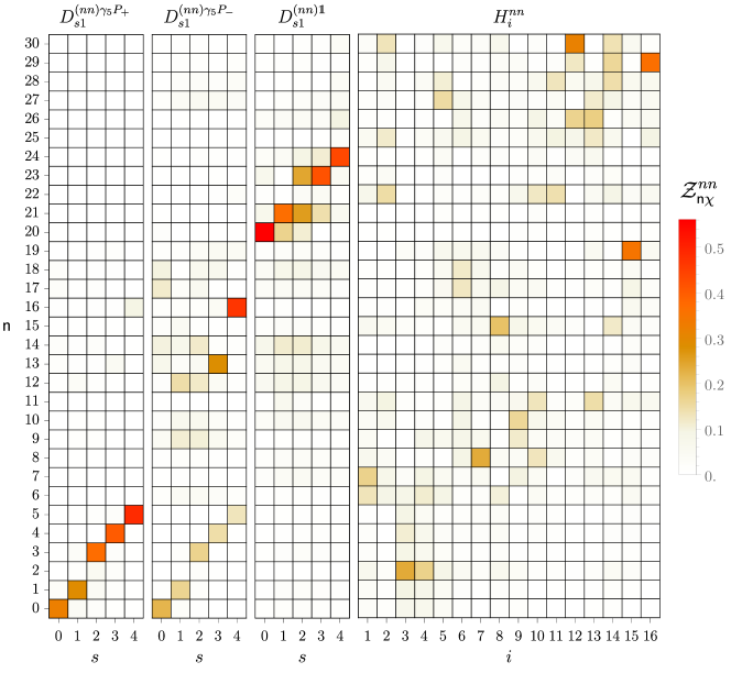
Figure 8: Results for relative overlap factors $\mathcal{Z}_{\mathsf{n}\chi}^{nn}$ for operator set $\mathbb{S}_{15D}^{nn}\cup\mathbb{S}_{16H}^{nn}$. Uncertainties are not shown here but are shown by error bars in histograms for the 6 lowest-energy states in Fig. 17.

One can now critically re-examine both the dibaryon-only and hexaquark-only operator sets. In particular, this study suggests that the hexaquark and dibaryon operators have statistically resolvable overlaps with disjoint sectors of the Hilbert space. This hypothesis is reinforced by examining the overlap factors obtained from fits to the operator set $\mathbb{S}_{15D}^{nn}\cup\mathbb{S}_{16H}^{nn}$, shown in Fig. 8 and Appendix C. There, it can be seen that the dibaryon operators have large relative overlap with energy-levels which sit near non-interacting two-nucleon energy levels ($\mathsf{n}\in\{0,1,3,4,5\}$), while the additional energy level ($\mathsf{n}=2$) has large relative overlap with the hexaquark operators $H_{3}^{nn}$ and $H_{4}^{nn}$. The existence of a low-lying energy level with small overlap to dibaryon operators has been previously observed at the same pion mass but different physical volume in Ref. [56].

It is noteworthy that there is not a simple diagnostic for the existence of a third energy level below $a\Delta E^{nn}\lesssim 0.1$ arising from analysis of $\mathbb{S}_{15D}^{nn}$ or for the existence of multiple energy levels below $\Delta_{\text{cut}}$ using $\mathbb{S}_{16H}^{nn}$. It is clear that computationally-accessible Euclidean times are not yet sufficient to ensure that all variational bounds are saturated within statistical uncertainties. Therefore, one should exercise caution in assuming that the bounds from a given interpolating-operator set are in one-to-one correspondence with energy levels.

The set $\mathbb{S}_{16H}^{nn}$ contains operators which cannot be written as the local product of two color-singlet three-quark operators. Such operators probe the hidden-color components of the two-nucleon wavefunction. While such operators do not provide strong variational bounds on the low-energy dineutron spectrum and exhibit large statistical fluctuations, evidence exists for states higher in the spectrum having statistically-significant overlaps with these novel operators. This can be seen in Fig. 8, where the relative overlaps of each GEVP eigenvector onto each operator is shown. In particular, the $\mathsf{n}=2$ dineutron level has largest overlaps with operators with $T^{AAS}$ color structures arising from products of two color-singlet baryon operators and includes an admixture of upper-spin-component and lower-spin-component operators of this form. Operators involving the color tensors $T^{AAA}$ and $T^{SSS}$ that cannot be constructed from products of color-singlet baryons are associated with the appearance of variational bounds above $\Delta_{\text{cut}}$. It is noteworthy that several of these variational bounds appear between $\Delta_{\text{cut}}$ and $a\delta E^{N^{+}}$, which suggests that hidden-color operators in this channel predominantly overlap with lower-energy states than operators involving single-nucleon excitations. The structure of these states may exhibit novel features associated with the presence of hidden color that should be explored in future work.

IV.3.2 The Deuteron Channel

Similar studies using the various operator sets can be performed for the deuteron channel. Results are presented for the $J_{z}=0$ row of the $T_{1}^{+}$ irrep, which contains the $\ell=0$ partial-wave contribution in the infinite volume limit. The resulting variational bounds on the spectra are shown in Figs. 9 and 10. It is important to note that unlike the dineutron channel, multiple linearly independent dibaryon interpolating operators in a given row of the cubic group representation can be constructed. These arise because the total angular momentum irrep is a tensor product of the “orbital” angular momentum and the spin, $\Gamma_{J}=\Gamma_{\ell}\otimes\Gamma_{\rm spin}$. The total-angular-momentum irrep containing the deuteron ($\Gamma_{J}=T_{1}^{+}$) includes contributions from spatial wavefunctions with $\Gamma_{\ell}\in\{A_{1}^{+},E^{+},T_{2}^{+}\}$ (other irreps are only relevant for higher-momentum dibaryon operators. For example, $\Gamma_{\ell}=T_{1}^{+}$ contributes for $s\geq 5$). Thus, these operators are sensitive to the energy splittings arising from the orbital angular momenta of the states. The multiplicities of operators with total angular momentum irrep $\Gamma_{J}$ are given in Table III of Ref. [56]. In particular, for $\Gamma_{J}=T_{1}^{+}$, the multiplicities are $N_{s}^{(0,T_{1}^{+})}=\{1,2,3,2,2\}$ for $s=\{0,1,2,3,4\}$, respectively. Consequently, if the low-energy deuteron spectrum could be described purely in terms of non-interacting energy levels, then one should expect $N_{s}^{(0,T_{1}^{+})}$ nearby variational bounds for each non-interacting energy level.

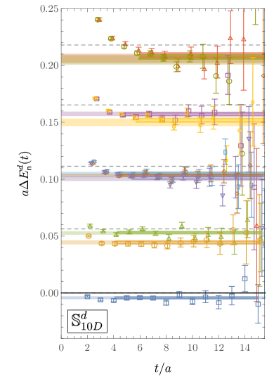
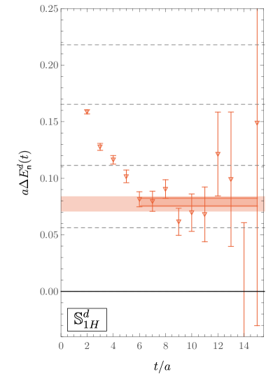
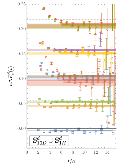
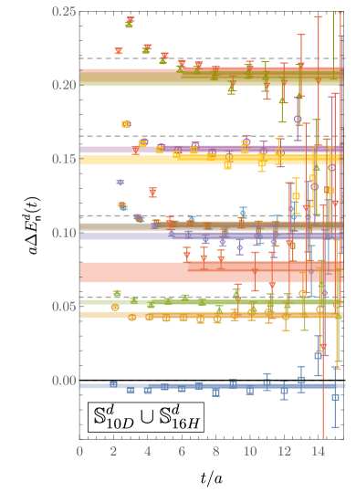
Figure 9: Effective mass spectra for operator sets $\mathbb{S}_{{10D}}^{{d}}$ (top left), $\mathbb{S}_{1H}^{{d}}$ (top right), $\mathbb{S}_{{10D}}^{{d}}\cup\mathbb{S}_{1H}^{d}$ (bottom left), and $\mathbb{S}_{{10D}}^{{d}}\cup\mathbb{S}_{16H}^{{d}}$ (bottom right) for the deuteron, $(B,I,\Gamma_{J})=(2,0,T_{1}^{+})$. Non-interacting $NN$ energy levels are represented as dashed horizontal lines.

Figure 10: Summary of low-lying deuteron $(B,I,\Gamma_{J})=(2,0,T_{1}^{+})$ spectra obtained from all operator sets considered in this work. Non-interacting $NN$ energy levels are represented as dashed horizontal lines.

For the operator sets containing only dibaryon operators ($\mathbb{S}_{{10D}}^{d}$, $\mathbb{S}_{{20D}}^{d}$, $\mathbb{S}_{{30D}}^{d}$), exactly $N_{s}^{(0,T_{1}^{+})}$ nearby variational bounds for each $s$ are observed, in agreement with the expected counting of non-interacting degenerate copies. It is interesting to note that the variational bounds for the two $s=1$ states differ by several standard deviations. If these variational bounds were saturated, these differences could be used to study $S$-$D$ partial-wave mixing [107, 49]. Additional variational bounds appearing only for $\mathbb{S}_{{20D}}^{d}$ and $\mathbb{S}_{{30D}}^{d}$ are present at higher energies that, as in the dineutron channel, are consistent with $2a\delta E^{N^{-}}$ and $a\delta E^{N^{+}}$, respectively, as shown in Fig. 11.

The sets $\mathbb{S}_{1H}^{d}$, $\mathbb{S}_{2H}^{d}$ and $\mathbb{S}_{16H}^{d}$ again provide much less-constraining variational bounds of the low-energy eigenvalues of the deuteron system than the dibaryon operator-sets, but the ${\sf n}=0$ effective mass function exhibits a plateau at $a\Delta E^{d}{\approx}0.06$ As in the dineutron channel, combinations of dibaryon and hexaquark operator sets ($\mathbb{S}_{{10D}}^{d}\cup\mathbb{S}_{1H}$, $\mathbb{S}_{{10D}}^{d}\cup\mathbb{S}_{2H}^{d}$, $\mathbb{S}_{{10D}}^{d}\cup\mathbb{S}_{16H}^{d}$ and $\mathbb{S}_{{30D}}^{d}\cup\mathbb{S}_{16H}^{d}$) produce spectral bounds that are approximately the union of the variational bounds of the spectra from the dibaryon-only and hexaquark-only operator sets. That is, in addition to the $N_{s}^{(0,T_{1}^{+})}$ variational bounds arising primarily from the dibaryon operators, there is an additional variational bound below $a\Delta E^{d}\lesssim 0.1$. This larger set of variational bounds therefore provides strong evidence for an additional energy eigenstate below this threshold. While the majority of the variational bounds arising predominantly from the dibaryon operators remain fairly stable between operator sets, this additional variational bound exhibits greater sensitivity to the choice of operators used.

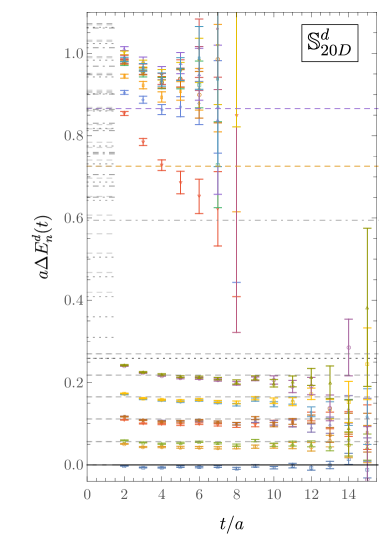
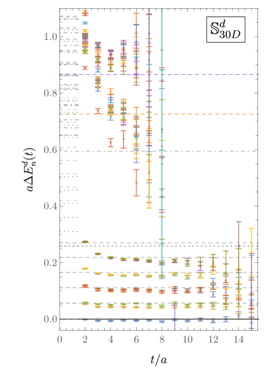
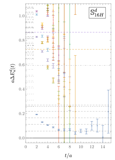
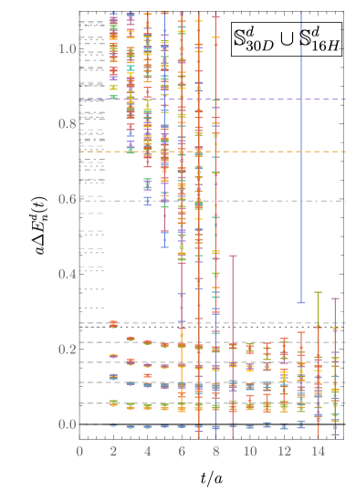
Figure 11: The effective mass spectra showing all of the variational bounds obtained with the interpolating-operator sets indicated. Non-interacting energy levels are represented as in Fig. 7 except that $N\Delta$ states are excluded from the deuteron channel by isospin.

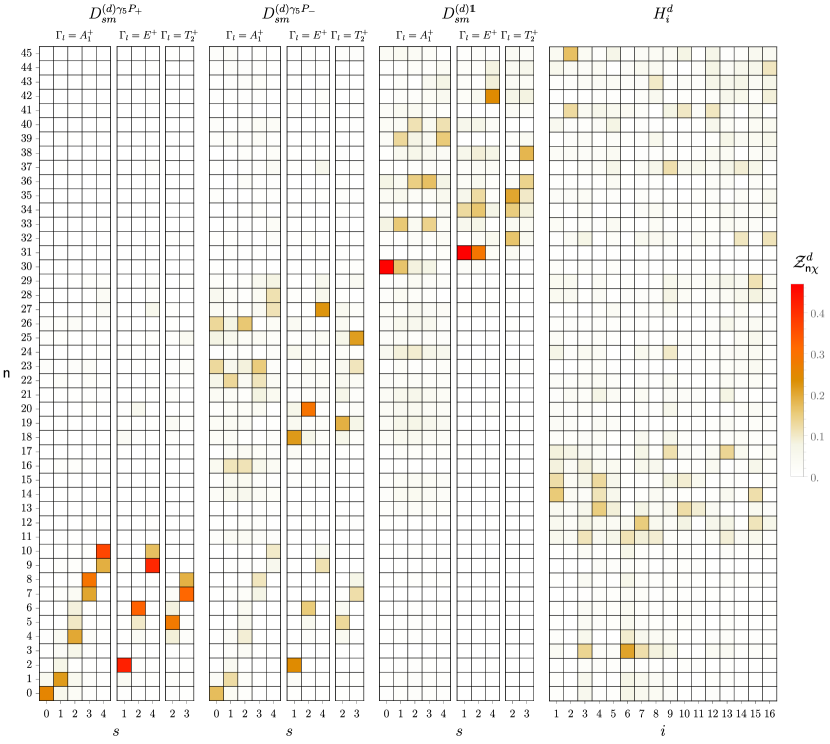
Figure 12: Results for relative overlap factors $\mathcal{Z}_{\mathsf{n}\chi}^{d}$ for the operator set $\mathbb{S}_{{30D}}^{d}\cup\mathbb{S}_{16H}^{d}$. Uncertainties are not shown here but are shown for the 11 lowest-energy states by the error bars in the histograms in Figs. 18-19.

Further understanding of these results can be obtained by examining the relative overlaps, shown in Fig. 12 and Appendix C. As in the dineutron channel, it can be seen that the dibaryon operators have large relative overlaps with GEVP eigenvectors whose eigenvalues are close to the non-interacting two-nucleon energy levels ($\mathsf{n}\in\{0,1,3,4,5\}$), while the additional energy level ($\mathsf{n}=2$) has large relative overlap with hexaquark operators $H_{6}^{d}$ and $H_{7}^{d}$ constructed from the $T^{AAS}$ color tensor. In contrast to the dineutron channel, the $\mathsf{n}=2$ level also has significant overlap with the hexaquark operator $H_{3}^{d}$, which involves the $T^{AAA}$ color tensor and therefore corresponds to hidden-color components of the deuteron. Additional GEVP eigenvectors have significant overlap with hexaquark operators with $T^{AAA}$ and $T^{SSS}$ color structures, but unlike the dineutron channel, most of these energy levels overlap with multiple hexaquark operators. The implications of this difference for the structures of states in the dineutron and deuteron channels require further study.

V Discussion

Variational bounds from operators sets involving both dibaryon and hexaquark operators ($\mathbb{S}_{15D}^{nn}\cup\mathbb{S}_{16H}^{nn}$ and $\mathbb{S}_{{30D}}^{d}\cup\mathbb{S}_{16H}^{d}$) strongly suggest the presence of an additional energy eigenvalue in both the dineutron and deuteron channels below $a\Delta E_{\mathsf{n}}^{Q}\lesssim 0.1$ ($Q\in\{nn,d\}$). These additional dineutron and deutron energy level are not present for two non-interacting nucleons and are too close to the two-nucleon threshold to be explained as $N\Delta$ or $\Delta\Delta$ scattering states. The present section explores the implications of these results.

The observation that the operator sets built purely from dibaryon operators such as $\mathbb{S}_{15D}^{nn}$ and $\mathbb{S}_{{30D}}^{d}$ are statistically insensitive to the additional state in each channel is similar to observations made in Ref. [122] in the context of the $\rho$ meson resonance in the $I=1$ $\pi\pi$ scattering channel. There, an operator set built from multiple back-to-back momentum-projected two-pion interpolating operators leads to energy bounds consistent with the number of non-interacting $\pi\pi$ scattering states expected below a given energy. The inclusion of $\rho$-like local interpolating operators into the operator set leads to an additional low-energy variational bound which in turn implies the existence of an additional energy eigenvalue beyond those related to the non-interacting spectrum. Calculations in multiple volumes and with boosted momentum-frames indicate that this eigenvalue corresponds to the $\rho$ resonance. Similar “missing-state” effects have also been seen in meson-baryon systems [123, 124]. Combining these previous observations with those here and in Ref. [56] in the two-nucleon system shows that it is not uncommon for variational studies with operator sets with many elements to provide misleading information on the spectrum if the energy bounds that arise are interpreted as energy determinations. In the context of the two-nucleon system, this means that conclusions regarding the absence of bound states at large quark masses (or about the number of finite-volume eigenstates with energies below any given threshold) must always be subject to the caveat that they could change dramatically with the inclusion of a single additional operator.

In order to make physical statements and predictions, quantities determined from LQCD calculation must be extrapolated to the continuum limit. Due to the use of a perturbatively-improved action in this study, the leading lattice artifacts in energies and energy-differences are expected to arise at $\mathcal{O}(g^{2}a\Lambda_{\rm QCD})$ and $\mathcal{O}(a^{2}\Lambda_{\rm QCD}^{2})$ (here, $g$ is the strong coupling at scale $\mu\sim 1/a$ and $\Lambda_{\rm QCD}\approx 0.3$ GeV is the typical QCD scale), both of which are $\lesssim 0.1$. However, since the current study is performed at a single lattice spacing, the magnitude of the lattice artifacts that are present has not been quantified. Given this, the possibility that the additional states inferred in both two-nucleon channels have large lattice artifacts which shift their energies to significantly different values than in the continuum cannot be ruled out. A quantitative study of lattice artifacts in the obtained variational bounds is left for future work. It should also be noted that significant changes between variational bounds at different lattice spacings do not necessarily imply significant differences between energy eigenvalues.

If lattice artifacts in the variational bounds on the additional states are assumed to be small, some further observations about the dineutron and deuteron spectra can be made. Firstly, the presence of this state in both channels, as opposed to only one, is natural in the heavy-quark limit, where heavy-quark spin symmetry implies that the two isospin channels are degenerate up to corrections which are suppressed by inverse powers of the heavy-quark mass [73]. This degeneracy can also be argued by noting that in the large-$N_{c}$ limit, nuclear interactions exhibit an $SU(4)$ Wigner spin-isospin symmetry [74]. In this limit, the dineutron and deuteron channels are expected to be degenerate, up to corrections suppressed by inverse powers of $N_{c}$.

The presence of additional states in the low-energy dineutron and deuteron spectra have also previously been observed in a calculation at the same pion mass in a volume with spatial extent $L=4.5~{}$\mathrm{f}\mathrm{m}$$ [56]. By combining the results obtained from operator set $\mathbb{S}_{0}$ in Ref. [56] (corresponding to 14 positive-parity, upper-spin-component dibaryon operators, plus a single $T^{AAS}$ hexaquark operator) with the results from this analysis, it is possible to study the volume dependence of variational bounds for the finite-volume spectra. This volume dependence is shown in Fig. 13 using the operator sets $\mathbb{S}_{15D}^{nn}\cup\mathbb{S}_{16H}^{nn}$ and $\mathbb{S}_{30D}^{d}\cup\mathbb{S}_{16H}^{d}$. It is interesting to note that the additional state exhibits weak volume dependence compared with the states that fall near the non-interacting levels and overlap strongly with the dibaryon operators. This is the behavior expected of a resonance rather than a scattering state [125].

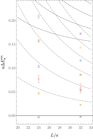
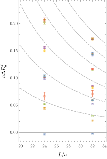
Figure 13: The strongest variational bounds achieved here in the dineutron and deuteron channels, compared to best variational bounds obtained at a larger volume in Ref. [56]. Non-interacting $NN$ and $N\Delta$ energy levels are represented as dashed and dotted lines, respectively.

Experimental evidence supports the existence of an isoscalar $J^{P}=3^{+}$ resonance in $I=0$ two-nucleon scattering, termed the $d^{*}(2380)$ [75, 76, 77, 78, 79]. If such a state persists at the heavy values of the quark masses used in the current work, it would appear in the $T_{1}^{+}$ irrep, since below the $\Delta\Delta$ threshold, the $T_{1}^{+}$ irrep can be written as the tensor product $\Gamma_{J}=\Gamma_{\ell}\otimes\Gamma_{\text{spin}}=A_{1}^{+}\otimes T_{1}^{+}$, which subduces from $(\ell=4)\otimes(S=1)$ and overlaps with states with total angular momentum and parity $J^{P}=3^{+}$. The additional state inferred from the variational bounds in the deuteron channel could be a heavy-quark-mass analog of the $d^{*}$ resonance. The similarities between the variational bounds in the deuteron and dineutron channels suggests the possibility of a corresponding $I=1$ two-nucleon resonance for these quark-mass values. The total angular momentum of such an $I=1$ resonance should be $J\in\{0,4,\ldots\}$ in order to appear in the $A_{1}^{+}$ irrep. The existence of such an $I=1$ resonance at physical quark masses is an interesting target for future study.

Having extracted variational bounds for the low-energy dineutron and deuteron spectra in two physical volumes, it is natural to attempt to compute the associated phase-shifts using the finite-volume quantization-conditions described in Refs. [58, 103, 126]. However, the Euclidean time extents over which statistically-significant signals for energy shifts have been extracted in the current study are smaller than the inverse of the energy gap between the lowest two finite-volume energy levels of non-interacting nucleons and are not sufficient to have confidence that any of the variational bounds have been saturated. One should therefore not assume that variational bounds are in one-to-one correspondence with energy eigenvalues. The interlacing theorem rigorously guarantees that at least $n$ energy eigenvalues sit below the $n$th variational bound, and these one-sided intervals can be mapped to one-sided intervals in the $(k^{2},k\cot\delta)$-plane using the quantization conditions. Due to the singularity structure of the quantization conditions, these intervals do not provide meaningful constraints on the phase shifts. Precise constraints can only be obtained by making the assumption that variational bounds are saturated and correspond to stochastic estimates of energy eigenvalues.

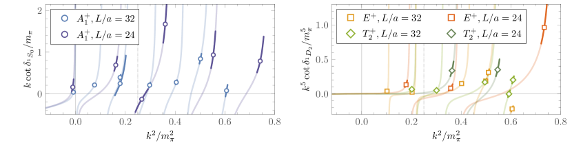
Figure 14: Values of the phase-shift from different irreps for the dineutron channel combining the results from this work ($L/a=24$) and Ref. [56] ($L/a=32$). The opaque lines represent the statistical and systematic uncertainties from the fit to the correlation matrix, while the translucent lines represent the bounds from the interlacing theorem. The vertical dot-dashed line indicates the radius of convergence of the effective range expansion due to the $t$-channel cut.

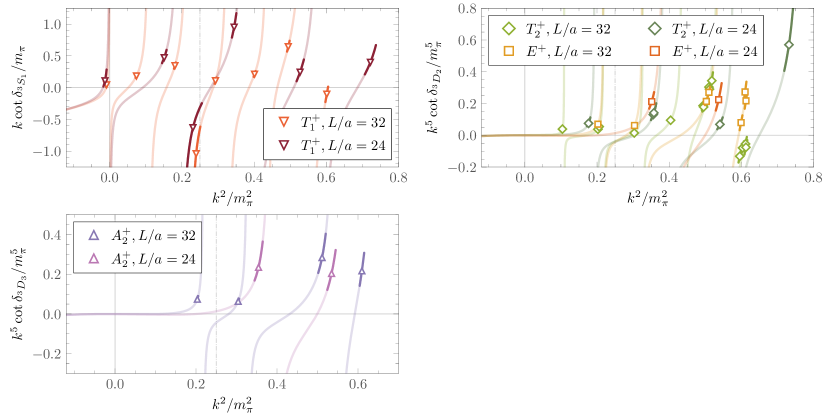
Figure 15: Values of the phase-shift from different irreps for the deuteron channel combining the results from this work ($L/a=24$) and Ref. [56] ($L/a=32$). Details are as in Fig. 14.

Assuming that only the lowest partial-wave contributes to a given cubic irrep (e.g., ${}^{1}S_{0}$ in $I=1$, $\Gamma=A_{1}^{+}$), one can obtain the corresponding phase-shifts, as shown in Figs. 14 and 15. Further details on the quantization conditions used here are discussed in Appendix G of Ref. [56]. Assuming saturation of the variational bounds, it is interesting to observe the rapid variation of the phase-shift around $k^{2}/m^{2}_{\pi}\sim 0.25$ in the $(I=1,A_{1}^{+})$ and $(I=0,T_{1}^{+})$ channels, close to the maximum radius of convergence of the effective range expansion. This is signaled primarily by the phase shifts corresponding to the GEVP eigenvectors with the largest relative overlap onto the hexaquark operators. This behavior is characteristic of a pole in the complex-energy plane, however, a more detailed analysis is required to extract information about the scattering amplitude and is left for future work. It is also interesting to note that most of the individual phase-shift determinations are insensitive to the presence of the hexaquark operators; they do not shift significantly if the set of operators does not include one or more hexaquark operators. Further information on the variational bounds obtained in this study may be obtained by studying the system in boosted frames. Such a study is left for a future work.

VI Summary and Outlook

In this work, the two-nucleon spectrum is studied using LQCD at quark masses corresponding to a pion mass of $m_{\pi}\approx 806~{}$\mathrm{M}\mathrm{e}\mathrm{V}$$ using the variational method, leading to bounds on the finite-volume energy eigenstates. The effects on the variational bounds for the two-nucleon spectrum from various choices of dibaryon operators and local hexaquark operators with both $I=0$ and $I=1$ are quantified. In particular, this study analyzes for the first time the impact of including products of negative-parity nucleon operators as well as dibaryon operators containing the lower-spin-components of quark fields. These operators lead to minimal changes to the low-energy variational bounds obtained using only upper-spin-component dibaryon operators. While operator sets which contain only hexaquark operators produce variational bounds of the low-energy spectrum that are much less constraining than those from operator sets which contain dibaryon operators, the combination of dibaryon and hexaquark operators provides strong evidence for the presence of an additional energy level below $a\Delta E\lesssim 0.1$ in both the deuteron and dineutron channels. The presence of this additional state was previously observed in Ref. [56] in a calculation with the same quark masses but a different physical volume. Including hexaquark operators describing hidden color two-nucleon states improves the precision of this bound and results in additional variational bounds appearing at somewhat higher energies. Particular hidden-color hexaquark operators make the only significant contributions to the overlap factors associated with some of these bounds, which suggests that there may be two-nucleon excited states with novel structure related to hidden-color components.

Since the calculations presented here are performed at a single lattice spacing, it is possible that the variational bounds contain significant lattice artifacts, and bounds could move in either direction as they approach the continuum limit. Further studies will explore the existence of such a state in the continuum limit and for physical quark masses.

Appendix A Choosing $t_{0}$ and $t_{\rm ref}$

As discussed in the main text, $t_{\text{ref}}$ and $t_{0}$ should be chosen so that the effective masses obtained using the eigenvector- and eigenvalue-based definitions of the principal correlation functions in Eqs. (16) and (17), respectively, agree within uncertainties. This is achieved using the following algorithm, shown in Fig. 16 with the algorithm parameters highlighted in blue.

• Set $t_{0}=\delta$ and $t_{\text{ref}}=t_{0}+\delta$, where $\delta$ is the minimum distance over which a sum-of-exponential spectral representation is expected to be valid.

• Verify that $\lambda_{\mathsf{n}}(t_{\text{ref}},t_{0})>0$ are positive. If not, the correlation-function matrix is approximately degenerate at this statistical precision, and either an operator must be removed to decrease the size of the correlation-function matrix or statistical precision must be increased.

• Check whether $E_{\mathsf{n}}(t,t_{0},t_{\text{ref}})\approx F_{\mathsf{n}}(t)$ for all $t$ where $\delta F_{\mathsf{n}}(t)<\text{tol}_{\lambda}\delta E_{\mathsf{n}}(t,t_{0},t_{\text{ref}})$ and $\approx$ denotes equality to within a combined statistical uncertainty of $\text{tol}_{\sigma}$. Here $\text{tol}_{\lambda}$ and $\text{tol}_{\sigma}$ are hyperparameters that are set to $\text{tol}_{\lambda}=1.5$ and $\text{tol}_{\sigma}=2\sigma$ for the calculations in this work. If this check is passed for all $n$ with $E_{\mathsf{n}}(t,t_{0},t_{\text{ref}})<\text{tol}_{E}$, then a “plateau region” of $t_{0}$ and $t_{\text{ref}}$ where the eigenvector- and eigenvalue-based principal correlation functions are consistent has been identified.

• Define $t_{0}^{\prime}=t_{0}+1$ and $t_{\text{ref}}^{\prime}=t_{0}^{\prime}+\delta$.

• Verify that $\lambda_{\mathsf{n}}(t_{\text{ref}}^{\prime},t_{0}^{\prime})>0$ are positive. If there is a negative eigenvalue, then if a plateau region has been found, $t_{0}$ is the largest acceptable value before noise sets in and $t_{0}^{\text{best}}\equiv t_{0}$ (if a plateau has not been found, then there is insufficient statistical precision to analyze the correlation-function matrix).

• Check whether $E_{\mathsf{n}}(t,t_{0}^{\prime},t_{\text{ref}}^{\prime})\approx F_{\mathsf{n}}(t)$ to with $\text{tol}_{\sigma}$ for all $t$ where $\delta F_{\mathsf{n}}(t)<\text{tol}_{\lambda}\delta E_{\mathsf{n}}(t,t_{0}^{\prime},t_{\text{ref}}^{\prime})$ and all $n$ with $E_{\mathsf{n}}(t,t_{0}^{\prime},t_{\text{ref}}^{\prime})<\text{tol}_{E}$. If so, a plateau region has been found. If they do not agree, then if a plateau region has been found, $t_{0}$ is the largest acceptable value before noise sets in and $t_{0}^{\text{best}}\equiv t_{0}$ (if a plateau has not been found, then there is insufficient statistical precision to analyze the correlation-function matrix).

• Take $t_{0}\rightarrow t_{0}+1$.

• Repeat the previous four steps until $t_{0}^{\text{best}}$ has been identified.

• Define $t_{\text{ref}}\rightarrow t_{\text{ref}}^{\prime}=t_{\text{ref}}+1$.

• Verify that $\lambda_{\mathsf{n}}(t_{\text{ref}}^{\prime},t_{0}^{\text{best}})>0$ are positive. If there is a negative eigenvalue, then $t_{\text{ref}}^{\text{best}}\equiv t_{\text{ref}}$.

• Check whether $E_{\mathsf{n}}(t,t_{0}^{\text{best}},t_{\text{ref}}^{\prime})\approx F_{\mathsf{n}}(t)$ to with $\text{tol}_{\sigma}$ for all $t$ where $\delta F_{\mathsf{n}}(t)<\text{tol}_{\lambda}\delta E_{\mathsf{n}}(t,t_{\text{ref}}^{\prime},t_{0}^{\prime})$ and all $n$ with $E_{\mathsf{n}}(t,t_{0}^{\prime},t_{\text{ref}}^{\prime})<\text{tol}_{E}$. If they do not agree, then $t_{\text{ref}}^{\text{best}}\equiv t_{\text{ref}}$.

• Take $t_{\text{ref}}\rightarrow t_{\text{ref}}+1$.

• Repeat the previous four steps until $t_{\text{ref}}^{\text{best}}$ has been identified.

The desired principal correlation functions are then defined as $\hat{C}_{\mathsf{n}}(t)\equiv\hat{C}_{\mathsf{n}}(t,t_{0}^{\text{best}},t_{\text{ref}}^{\text{best}})$, and the associated effective mass functions are denoted $E_{\mathsf{n}}(t)\equiv E_{\mathsf{n}}(t,t_{0}^{\text{best}},t_{\text{ref}}^{\text{best}})$.

Figure 16: Flow chart representing the steps of the algorithm to find the best $t_{0}$ and $t_{\rm ref}$.

Appendix B Variational bounds

The strongest variational bounds for each of the one- and two-nucleon channels that are studied in this work are presented in Tables 5-7. Fits are performed using methods adapted from Refs. [51, 56] and the $t_{0}$, $t_{\text{ref}}$ selection criteria described in the main text and Appendix A. The uncertainties shown for $aE_{\mathsf{n}}^{Q}$ and $a\Delta E_{\mathsf{n}}^{Q}$ include systematic uncertainties associated with the variation in fit results obtained with different choices of $t_{\rm min}$ (the minimum temporal extent used in the fit) added in quadrature to statistical uncertainties calculated using bootstrap methods. Results for energies in physical units include uncertainties in the determination of $a=0.1453(16)$ fm [46] added in quadrature. Ambiguities in defining the lattice spacing away from the physical values of the quark masses are not quantified.

$n$	$aE_{\mathsf{n}}^{(1,\frac{1}{2},G_{1}^{+})}$	$E_{\mathsf{n}}^{(1,\frac{1}{2},G_{1}^{+})}\text{ [GeV]}$
0	$1.2027(25)$	$1.637(23)$
1	$1.9285(472)$	$2.624(74)$

$n$	$aE_{\mathsf{n}}^{(1,\frac{1}{2},G_{1}^{-})}$	$E_{\mathsf{n}}^{(1,\frac{1}{2},G_{1}^{-})}\text{ [GeV]}$
0	$1.6357(76)$	$2.226(32)$

Table 5: Single-nucleon positive- and negative-parity variational bounds in lattice and physical units obtained from weighted averages of multi-exponential fits to GEVP correlation functions as described in the main text.

$n$	$aE_{\mathsf{n}}^{(2,1,A_{1}^{+})}$	$a\Delta E_{\mathsf{n}}^{(2,1,A_{1}^{+})}$	$\Delta E_{\mathsf{n}}^{(2,1,A_{1}^{+})}\text{ [MeV]}$
0	$2.4035(38)$	$-0.0034(11)$	$-4.6(1.5)$
1	$2.4534(39)$	$0.0469(19)$	$63.9(2.7)$
2	$2.4809(97)$	$0.0768(75)$	$104.5(10.3)$
3	$2.5100(42)$	$0.1035(24)$	$140.9(3.8)$
4	$2.5627(46)$	$0.1571(24)$	$213.8(4.4)$
5	$2.6133(55)$	$0.2087(36)$	$284.0(6.3)$

$n$	$aE_{\mathsf{n}}^{(2,1,E^{+})}$	$a\Delta E_{\mathsf{n}}^{(2,1,E^{+})}$	$\Delta E_{\mathsf{n}}^{(2,1,E^{+})}\text{ [MeV]}$
0	$2.4584(41)$	$0.0518(14)$	$70.5(2.1)$
1	$2.5097(45)$	$0.1027(22)$	$139.8(3.5)$
2	$2.6134(55)$	$0.2063(32)$	$280.7(5.9)$

$n$	$aE_{\mathsf{n}}^{(2,1,T_{2}^{+})}$	$a\Delta E_{\mathsf{n}}^{(2,1,T_{2}^{+})}$	$\Delta E_{\mathsf{n}}^{(2,1,T_{2}^{+})}\text{ [MeV]}$
0	$2.5111(42)$	$0.1042(18)$	$141.8(3.1)$
1	$2.5620(45)$	$0.1554(20)$	$211.5(4.0)$

Table 6: Two-nucleon $I=1$ variational bounds in positive-parity total-angular-momentum cubic irreps $\Gamma_{J}\in\{A_{1}^{+},E^{+},T_{2}^{+}\}$ analogous to the results in Table 5. The interpolating-operator set $\mathbb{S}_{15D}^{nn}\cup\mathbb{S}_{16H}^{nn}$ is used.

$n$	$aE_{\mathsf{n}}^{(2,0,T_{1}^{+})}$	$a\Delta E_{\mathsf{n}}^{(2,0,T_{1}^{+})}$	$\Delta E_{\mathsf{n}}^{(2,0,T_{1}^{+})}\text{ [MeV]}$
0	$2.4029(39)$	$-0.0039(13)$	$-5.3(1.8)$
1	$2.4504(40)$	$0.0440(18)$	$59.9(2.6)$
2	$2.4596(40)$	$0.0528(13)$	$71.8(2.1)$
3	$2.4708(87)$	$0.0663(74)$	$90.3(10.1)$
4	$2.5055(42)$	$0.0991(18)$	$134.8(3.1)$
5	$2.5101(46)$	$0.1034(23)$	$140.7(3.7)$
6	$2.5114(42)$	$0.1041(18)$	$141.7(3.1)$
7	$2.5570(52)$	$0.1501(27)$	$204.2(4.7)$
8	$2.5626(42)$	$0.1559(19)$	$212.1(3.9)$
9	$2.6084(63)$	$0.2030(44)$	$276.3(7.0)$
10	$2.6117(61)$	$0.2064(40)$	$280.9(6.7)$

$n$	$aE_{\mathsf{n}}^{(2,0,T_{2}^{+})}$	$a\Delta E_{\mathsf{n}}^{(2,0,T_{2}^{+})}$	$\Delta E_{\mathsf{n}}^{(2,0,T_{2}^{+})}\text{ [MeV]}$
0	$2.4577(42)$	$0.0513(14)$	$69.8(2.1)$
1	$2.5085(47)$	$0.1022(19)$	$139.0(3.2)$
2	$2.5093(46)$	$0.1026(20)$	$139.7(3.3)$
3	$2.5598(49)$	$0.1537(21)$	$209.2(4.1)$
4	$2.6121(54)$	$0.2059(35)$	$280.2(6.1)$

$n$	$aE_{\mathsf{n}}^{(2,0,E^{+})}$	$a\Delta E_{\mathsf{n}}^{(2,0,E^{+})}$	$\Delta E_{\mathsf{n}}^{(2,0,E^{+})}\text{ [MeV]}$
0	$2.5079(43)$	$0.1010(20)$	$137.5(3.3)$
1	$2.5595(44)$	$0.1526(22)$	$207.7(4.2)$

$n$	$aE_{\mathsf{n}}^{(2,0,A_{2}^{+})}$	$a\Delta E_{\mathsf{n}}^{(2,0,A_{2}^{+})}$	$\Delta E_{\mathsf{n}}^{(2,0,A_{2}^{+})}\text{ [MeV]}$
0	$2.5081(51)$	$0.1018(28)$	$138.6(4.3)$
1	$2.5575(62)$	$0.1520(30)$	$206.9(5.0)$

Table 7: Two-nucleon $I=0$ variational bounds in positive-parity total-angular-momentum cubic irreps $\Gamma_{J}\in\{T_{1}^{+},T_{2}^{+},E^{+},A_{2}^{+}\}$ analogous to the results in Table 5. The interpolating-operator set $\mathbb{S}_{30D}^{d}\cup\mathbb{S}_{16H}^{d}$ is used.

Appendix C Effective masses and overlaps

This appendix presents more details on the effective mass functions and overlaps associated with variational bounds below $\Delta_{\text{cut}}$. Effective masses for the dineutron channel, which are shown collectively in Fig. 5, are shown individually in more detail in Fig. 17. The corresponding overlap factors, whose central values are indicated in Fig. 8, are also shown here as histograms with error bars. Analogous results for the deuteron channel are shown in Figs. 18 and 19.

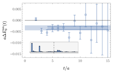
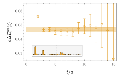
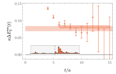
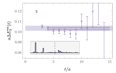
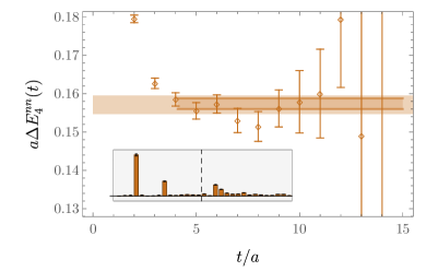
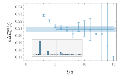
Figure 17: Results for two-nucleon GEVP effective FV energy shifts for the dineutron channel from the $\mathbb{S}_{15D}^{nn}\cup\mathbb{S}_{16H}^{nn}$ operator set. Histograms show the overlaps with interpolating operators corresponding to $s\in\{0,\ldots,4\}$ shell dibaryons with upper/lower/negative-parity spin components (15 bars left of dashed line) and a complete basis of hexaquarks (16 bars right of dashed line) ordered as in Fig. 8.

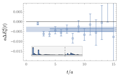
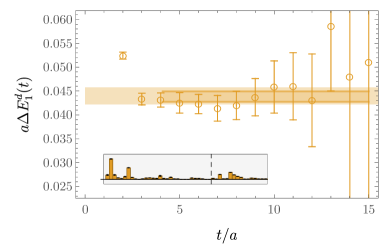
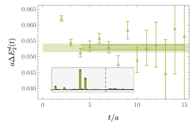
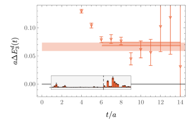
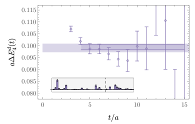
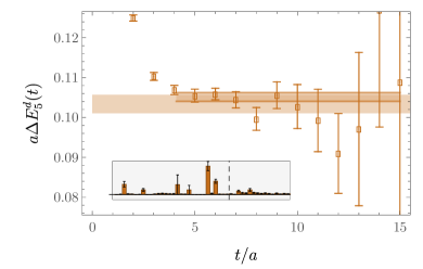
Figure 18: Results for two-nucleon GEVP effective FV energy shifts for the deuteron channel from the $\mathbb{S}_{30D}^{d}\cup\mathbb{S}_{16H}^{d}$ operator set. Histograms show the overlaps with interpolating operators corresponding to $s\in\{0,\ldots,4\}$ shell dibaryons with upper/lower/negative-parity spin components (30 bars left of dashed line) and a complete basis of hexaquarks (16 bars right of dashed line) ordered as in Fig. 12.

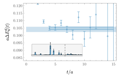
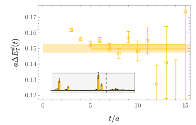
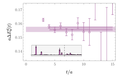
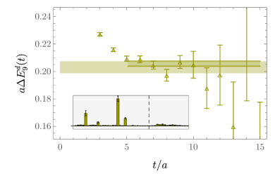
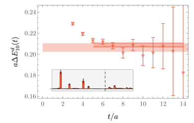
Figure 19: Additional results for two-nucleon GEVP effective FV energy shifts for the deuteron channel. Details are as in Fig. 18.

References

- Detmold et al. [2019] William Detmold, Robert G. Edwards, Jozef J. Dudek, Michael Engelhardt, Huey-Wen Lin, Stefan Meinel, Kostas Orginos, and Phiala Shanahan (USQCD), “Hadrons and Nuclei,” Eur. Phys. J. A 55, 193 (2019), arXiv:1904.09512 [hep-lat] .
- Drischler et al. [2019] Christian Drischler, Wick Haxton, Kenneth McElvain, Emanuele Mereghetti, Amy Nicholson, Pavlos Vranas, and André Walker-Loud, “Towards grounding nuclear physics in QCD,” (2019) arXiv:1910.07961 [nucl-th] .
- Davoudi et al. [2021] Zohreh Davoudi, William Detmold, Kostas Orginos, Assumpta Parreño, Martin J. Savage, Phiala Shanahan, and Michael L. Wagman, “Nuclear matrix elements from lattice QCD for electroweak and beyond-Standard-Model processes,” Phys. Rept. 900, 1–74 (2021), arXiv:2008.11160 [hep-lat] .
- Tews et al. [2022] Ingo Tews et al., “Nuclear Forces for Precision Nuclear Physics: A Collection of Perspectives,” Few Body Syst. 63, 67 (2022), arXiv:2202.01105 [nucl-th] .
- Kronfeld et al. [2022] Andreas S. Kronfeld et al. (USQCD), “Lattice QCD and Particle Physics,” (2022), arXiv:2207.07641 [hep-lat] .
- Prezeau et al. [2003a] Gary Prezeau, Andriy Kurylov, Marc Kamionkowski, and Petr Vogel, “New contribution to wimp-nucleus scattering,” Phys. Rev. Lett. 91, 231301 (2003a), arXiv:astro-ph/0309115 .
- Chang et al. [2018] Emmanuel Chang, Zohreh Davoudi, William Detmold, Arjun S. Gambhir, Kostas Orginos, Martin J. Savage, Phiala E. Shanahan, Michael L. Wagman, and Frank Winter (NPLQCD), “Scalar, Axial, and Tensor Interactions of Light Nuclei from Lattice QCD,” Phys. Rev. Lett. 120, 152002 (2018), arXiv:1712.03221 [hep-lat] .
- Krebs et al. [2020] Hermann Krebs, Evgeny Epelbaum, and Ulf-G. Meißner, “Subleading contributions to the nuclear scalar isoscalar current,” Eur. Phys. J. A 56, 240 (2020), arXiv:2005.07433 [nucl-th] .
- de Vries et al. [2023] J. de Vries, C. Körber, A. Nogga, and S. Shain, “Dark matter scattering off 4He in chiral effective field theory,” (2023), arXiv:2310.11343 [hep-ph] .
- Prezeau et al. [2003b] Gary Prezeau, M. Ramsey-Musolf, and Petr Vogel, “Neutrinoless double beta decay and effective field theory,” Phys. Rev. D 68, 034016 (2003b), arXiv:hep-ph/0303205 .
- Cirigliano et al. [2021] Vincenzo Cirigliano, Wouter Dekens, Jordy de Vries, Martin Hoferichter, and Emanuele Mereghetti, “Toward Complete Leading-Order Predictions for Neutrinoless Double Decay,” Phys. Rev. Lett. 126, 172002 (2021), arXiv:2012.11602 [nucl-th] .
- Cirigliano et al. [2022] V. Cirigliano et al., “Towards precise and accurate calculations of neutrinoless double-beta decay,” J. Phys. G 49, 120502 (2022), arXiv:2207.01085 [nucl-th] .
- Davoudi et al. [2024] Zohreh Davoudi, William Detmold, Zhenghao Fu, Anthony V. Grebe, William Jay, David Murphy, Patrick Oare, Phiala E. Shanahan, and Michael L. Wagman, “Long-Distance Nuclear Matrix Elements for Neutrinoless Double-Beta Decay from Lattice QCD,” (2024), arXiv:2402.09362 [hep-lat] .
- Alvarez-Ruso et al. [2018] L. Alvarez-Ruso et al. (NuSTEC), “NuSTEC White Paper: Status and challenges of neutrino–nucleus scattering,” Prog. Part. Nucl. Phys. 100, 1–68 (2018), arXiv:1706.03621 [hep-ph] .
- Kronfeld et al. [2019] Andreas S. Kronfeld, David G. Richards, William Detmold, Rajan Gupta, Huey-Wen Lin, Keh-Fei Liu, Aaron S. Meyer, Raza Sufian, and Sergey Syritsyn (USQCD), “Lattice QCD and Neutrino-Nucleus Scattering,” Eur. Phys. J. A 55, 196 (2019), arXiv:1904.09931 [hep-lat] .
- Ruso et al. [2022] L. Alvarez Ruso et al., “Theoretical tools for neutrino scattering: interplay between lattice QCD, EFTs, nuclear physics, phenomenology, and neutrino event generators,” (2022), arXiv:2203.09030 [hep-ph] .
- Kronfeld [2012] Andreas S. Kronfeld, “Twenty-first Century Lattice Gauge Theory: Results from the QCD Lagrangian,” Ann. Rev. Nucl. Part. Sci. 62, 265–284 (2012), arXiv:1203.1204 [hep-lat] .
- Beane et al. [2011] S. R. Beane, W. Detmold, K. Orginos, and M. J. Savage, “Nuclear Physics from Lattice QCD,” Prog. Part. Nucl. Phys. 66, 1–40 (2011), arXiv:1004.2935 [hep-lat] .
- Briceño et al. [2018] Raul A. Briceño, Jozef J. Dudek, and Ross D. Young, “Scattering processes and resonances from lattice QCD,” Rev. Mod. Phys. 90, 025001 (2018), arXiv:1706.06223 [hep-lat] .
- Hansen and Sharpe [2019] Maxwell T. Hansen and Stephen R. Sharpe, “Lattice QCD and Three-particle Decays of Resonances,” Ann. Rev. Nucl. Part. Sci. 69, 65–107 (2019), arXiv:1901.00483 [hep-lat] .
- Hörz [2022] Ben Hörz, “Spectroscopy and Hadron Interactions,” PoS LATTICE2021, 006 (2022).
- Romero-López [2023] Fernando Romero-López, “Multi-hadron interactions from lattice QCD,” PoS LATTICE2022, 235 (2023), arXiv:2212.13793 [hep-lat] .
- Hanlon [2024] Andrew D. Hanlon, “Hadron spectroscopy and few-body dynamics from lattice QCD,” in 40th International Symposium on Lattice Field Theory (2024) arXiv:2402.05185 [hep-lat] .
- Parisi [1984] G. Parisi, “The Strategy for Computing the Hadronic Mass Spectrum,” Phys. Rept. 103, 203–211 (1984).
- Lepage [1989] G. Peter Lepage, “The Analysis of Algorithms for Lattice Field Theory,” in Theoretical Advanced Study Institute in Elementary Particle Physics (1989).
- Beane et al. [2009a] Silas R. Beane, William Detmold, Thomas C Luu, Kostas Orginos, Assumpta Parreño, Martin J. Savage, Aaron Torok, and Andre Walker-Loud (NPLQCD), “High Statistics Analysis using Anisotropic Clover Lattices: (II) Three-Baryon Systems,” Phys. Rev. D 80, 074501 (2009a), arXiv:0905.0466 [hep-lat] .
- Beane and Savage [2003a] Silas R. Beane and Martin J. Savage, “Variation of fundamental couplings and nuclear forces,” Nucl. Phys. A 713, 148–164 (2003a), arXiv:hep-ph/0206113 .
- Epelbaum et al. [2003] Evgeny Epelbaum, Ulf-G. Meißner, and Walter Gloeckle, “Nuclear forces in the chiral limit,” Nucl. Phys. A 714, 535–574 (2003), arXiv:nucl-th/0207089 .
- Beane and Savage [2003b] Silas R. Beane and Martin J. Savage, “The Quark mass dependence of two nucleon systems,” Nucl. Phys. A 717, 91–103 (2003b), arXiv:nucl-th/0208021 .
- Braaten and Hammer [2003] Eric Braaten and H. W. Hammer, “An Infrared renormalization group limit cycle in QCD,” Phys. Rev. Lett. 91, 102002 (2003), arXiv:nucl-th/0303038 .
- Flambaum and Wiringa [2007] V. V. Flambaum and Robert B. Wiringa, “Dependence of nuclear binding on hadronic mass variation,” Phys. Rev. C 76, 054002 (2007), arXiv:0709.0077 [nucl-th] .
- Bedaque et al. [2011] Paulo F. Bedaque, Thomas Luu, and Lucas Platter, “Quark mass variation constraints from Big Bang nucleosynthesis,” Phys. Rev. C 83, 045803 (2011), arXiv:1012.3840 [nucl-th] .
- Chen et al. [2012] Jiunn-Wei Chen, Tze-Kei Lee, C. P. Liu, and Yu-Sheng Liu, “On the Quark Mass Dependence of Two Nucleon Observables,” Phys. Rev. C 86, 054001 (2012), arXiv:1012.0453 [nucl-th] .
- Soto and Tarrus [2012] Joan Soto and Jaume Tarrus, “On the quark mass dependence of nucleon-nucleon S-wave scattering lengths,” Phys. Rev. C 85, 044001 (2012), arXiv:1112.4426 [nucl-th] .
- Epelbaum et al. [2013] Evgeny Epelbaum, Hermann Krebs, Timo A. Lähde, Dean Lee, and Ulf-G. Meißner, “Viability of Carbon-Based Life as a Function of the Light Quark Mass,” Phys. Rev. Lett. 110, 112502 (2013), arXiv:1212.4181 [nucl-th] .
- Detmold et al. [2014a] William Detmold, Matthew McCullough, and Andrew Pochinsky, “Dark Nuclei I: Cosmology and Indirect Detection,” Phys. Rev. D 90, 115013 (2014a), arXiv:1406.2276 [hep-ph] .
- Detmold et al. [2014b] William Detmold, Matthew McCullough, and Andrew Pochinsky, “Dark nuclei. II. Nuclear spectroscopy in two-color QCD,” Phys. Rev. D 90, 114506 (2014b), arXiv:1406.4116 [hep-lat] .
- DeGrand and Neil [2020] Thomas DeGrand and Ethan T. Neil, “Repurposing lattice QCD results for composite phenomenology,” Phys. Rev. D 101, 034504 (2020), arXiv:1910.08561 [hep-ph] .
- Fukugita et al. [1994] M. Fukugita, Y. Kuramashi, H. Mino, M. Okawa, and A. Ukawa, “An Exploratory study of nucleon-nucleon scattering lengths in lattice QCD,” Phys. Rev. Lett. 73, 2176–2179 (1994), arXiv:hep-lat/9407012 .
- Fukugita et al. [1995] M. Fukugita, Y. Kuramashi, M. Okawa, H. Mino, and A. Ukawa, “Hadron scattering lengths in lattice QCD,” Phys. Rev. D 52, 3003–3023 (1995), arXiv:hep-lat/9501024 .
- Beane et al. [2006] S. R. Beane, P. F. Bedaque, K. Orginos, and M. J. Savage, “Nucleon-nucleon scattering from fully-dynamical lattice QCD,” Phys. Rev. Lett. 97, 012001 (2006), arXiv:hep-lat/0602010 .
- Beane et al. [2007] Silas R. Beane, Paulo F. Bedaque, Thomas C. Luu, Kostas Orginos, Elisabetta Pallante, Assumpta Parreño, and Martin J. Savage (NPLQCD), “Hyperon-Nucleon Scattering from Fully-Dynamical Lattice QCD,” Nucl. Phys. A 794, 62–72 (2007), arXiv:hep-lat/0612026 .
- Beane et al. [2010] Silas R. Beane, William Detmold, Huey-Wen Lin, Thomas C. Luu, Kostas Orginos, Martin J. Savage, Aaron Torok, and Andre Walker-Loud (NPLQCD), “High Statistics Analysis using Anisotropic Clover Lattices: (III) Baryon-Baryon Interactions,” Phys. Rev. D 81, 054505 (2010), arXiv:0912.4243 [hep-lat] .
- Yamazaki et al. [2010] T. Yamazaki, Y. Kuramashi, and A. Ukawa (PACS-CS), “Helium Nuclei in Quenched Lattice QCD,” Phys. Rev. D 81, 111504 (2010), arXiv:0912.1383 [hep-lat] .
- Beane et al. [2012] S. R. Beane, E. Chang, W. Detmold, H. W. Lin, T. C. Luu, K. Orginos, A. Parreño, M. J. Savage, A. Torok, and A. Walker-Loud (NPLQCD), “The Deuteron and Exotic Two-Body Bound States from Lattice QCD,” Phys. Rev. D 85, 054511 (2012), arXiv:1109.2889 [hep-lat] .
- Beane et al. [2013a] S. R. Beane, E. Chang, S. D. Cohen, William Detmold, H. W. Lin, T. C. Luu, K. Orginos, A. Parreño, M. J. Savage, and A. Walker-Loud (NPLQCD), “Light Nuclei and Hypernuclei from Quantum Chromodynamics in the Limit of SU(3) Flavor Symmetry,” Phys. Rev. D 87, 034506 (2013a), arXiv:1206.5219 [hep-lat] .
- Beane et al. [2013b] S. R. Beane et al. (NPLQCD), “Nucleon-Nucleon Scattering Parameters in the Limit of SU(3) Flavor Symmetry,” Phys. Rev. C 88, 024003 (2013b), arXiv:1301.5790 [hep-lat] .
- Wagman et al. [2017] Michael L. Wagman, Frank Winter, Emmanuel Chang, Zohreh Davoudi, William Detmold, Kostas Orginos, Martin J. Savage, and Phiala E. Shanahan, “Baryon-Baryon Interactions and Spin-Flavor Symmetry from Lattice Quantum Chromodynamics,” Phys. Rev. D 96, 114510 (2017), arXiv:1706.06550 [hep-lat] .
- Orginos et al. [2015] Kostas Orginos, Assumpta Parreño, Martin J. Savage, Silas R. Beane, Emmanuel Chang, and William Detmold, “Two nucleon systems at from lattice QCD,” Phys. Rev. D 92, 114512 (2015), [Erratum: Phys.Rev.D 102, 039903 (2020)], arXiv:1508.07583 [hep-lat] .
- Beane et al. [2021] S. R. Beane et al. (NPLQCD, QCDSF), “Charged multihadron systems in lattice QCD+QED,” Phys. Rev. D 103, 054504 (2021), arXiv:2003.12130 [hep-lat] .
- Illa et al. [2021] Marc Illa et al. (NPLQCD), “Low-energy scattering and effective interactions of two baryons at MeV from lattice quantum chromodynamics,” Phys. Rev. D 103, 054508 (2021), arXiv:2009.12357 [hep-lat] .
- Yamazaki et al. [2012] Takeshi Yamazaki, Ken-ichi Ishikawa, Yoshinobu Kuramashi, and Akira Ukawa, “Helium nuclei, deuteron and dineutron in 2+1 flavor lattice QCD,” Phys. Rev. D 86, 074514 (2012), arXiv:1207.4277 [hep-lat] .
- Yamazaki et al. [2015] Takeshi Yamazaki, Ken-ichi Ishikawa, Yoshinobu Kuramashi, and Akira Ukawa, “Study of quark mass dependence of binding energy for light nuclei in 2+1 flavor lattice QCD,” Phys. Rev. D 92, 014501 (2015), arXiv:1502.04182 [hep-lat] .
- Berkowitz et al. [2017] Evan Berkowitz, Thorsten Kurth, Amy Nicholson, Balint Joó, Enrico Rinaldi, Mark Strother, Pavlos M. Vranas, and Andre Walker-Loud, “Two-Nucleon Higher Partial-Wave Scattering from Lattice QCD,” Phys. Lett. B 765, 285–292 (2017), arXiv:1508.00886 [hep-lat] .
- Francis et al. [2019] A. Francis, J. R. Green, P. M. Junnarkar, Ch. Miao, T. D. Rae, and H. Wittig, “Lattice QCD study of the dibaryon using hexaquark and two-baryon interpolators,” Phys. Rev. D 99, 074505 (2019), arXiv:1805.03966 [hep-lat] .
- Amarasinghe et al. [2023] Saman Amarasinghe, Riyadh Baghdadi, Zohreh Davoudi, William Detmold, Marc Illa, Assumpta Parreño, Andrew V. Pochinsky, Phiala E. Shanahan, and Michael L. Wagman, “Variational study of two-nucleon systems with lattice QCD,” Phys. Rev. D 107, 094508 (2023), arXiv:2108.10835 [hep-lat] .
- Hörz et al. [2021] Ben Hörz et al., “Two-nucleon S-wave interactions at the flavor-symmetric point with : A first lattice QCD calculation with the stochastic Laplacian Heaviside method,” Phys. Rev. C 103, 014003 (2021), arXiv:2009.11825 [hep-lat] .
- Lüscher [1986] M. Lüscher, “Volume Dependence of the Energy Spectrum in Massive Quantum Field Theories. 2. Scattering States,” Commun. Math. Phys. 105, 153–188 (1986).
- Lin et al. [2001] C. J. David Lin, G. Martinelli, Christopher T. Sachrajda, and M. Testa, “K – pi pi decays in a finite volume,” Nucl. Phys. B 619, 467–498 (2001), arXiv:hep-lat/0104006 .
- Aoki et al. [2005] S. Aoki et al. (CP-PACS), “I=2 pion scattering length from two-pion wave functions,” Phys. Rev. D 71, 094504 (2005), arXiv:hep-lat/0503025 .
- Ishii et al. [2007] N. Ishii, S. Aoki, and T. Hatsuda, “The Nuclear Force from Lattice QCD,” Phys. Rev. Lett. 99, 022001 (2007), arXiv:nucl-th/0611096 .
- Murano et al. [2011] Keiko Murano, Noriyoshi Ishii, Sinya Aoki, and Tetsuo Hatsuda, “Nucleon-Nucleon Potential and its Non-locality in Lattice QCD,” Prog. Theor. Phys. 125, 1225–1240 (2011), arXiv:1103.0619 [hep-lat] .
- Aoki et al. [2011] Sinya Aoki, Noriyoshi Ishii, Takumi Doi, Tetsuo Hatsuda, Yoichi Ikeda, Takashi Inoue, Keiko Murano, Hidekatsu Nemura, and Kenji Sasaki (HAL QCD), “Extraction of Hadron Interactions above Inelastic Threshold in Lattice QCD,” Proc. Japan Acad. B 87, 509–517 (2011), arXiv:1106.2281 [hep-lat] .
- Ishii et al. [2012] Noriyoshi Ishii, Sinya Aoki, Takumi Doi, Tetsuo Hatsuda, Yoichi Ikeda, Takashi Inoue, Keiko Murano, Hidekatsu Nemura, and Kenji Sasaki (HAL QCD), “Hadron–hadron interactions from imaginary-time Nambu–Bethe–Salpeter wave function on the lattice,” Phys. Lett. B 712, 437–441 (2012), arXiv:1203.3642 [hep-lat] .
- Sasaki et al. [2020] Kenji Sasaki et al. (HAL QCD), “ and N interactions from lattice QCD near the physical point,” Nucl. Phys. A 998, 121737 (2020), arXiv:1912.08630 [hep-lat] .
- Fox et al. [1982] G. Fox, R. Gupta, O. Martin, and S. Otto, “Monte Carlo Estimates of the Mass Gap of the O(2) and O(3) Spin Models in (1+1)-dimensions,” Nucl. Phys. B 205, 188–220 (1982).
- Michael and Teasdale [1983] Christopher Michael and I. Teasdale, “Extracting Glueball Masses From Lattice QCD,” Nucl. Phys. B 215, 433–446 (1983).
- Lüscher and Wolff [1990] Martin Lüscher and Ulli Wolff, “How to Calculate the Elastic Scattering Matrix in Two-dimensional Quantum Field Theories by Numerical Simulation,” Nucl. Phys. B 339, 222–252 (1990).
- Brodsky et al. [1983] Stanley J. Brodsky, Chueng-Ryong Ji, and G. Peter Lepage, “Quantum Chromodynamic Predictions for the Deuteron Form-Factor,” Phys. Rev. Lett. 51, 83 (1983).
- Miller [1984] G. A. Miller, “Six Quark Cluster Components of Nuclear Wave Functions and the Pion Nucleus Double Charge Exchange Reaction,” Phys. Rev. Lett. 53, 2008–2011 (1984).
- Bashkanov et al. [2013] M. Bashkanov, Stanley J. Brodsky, and H. Clement, “Novel Six-Quark Hidden-Color Dibaryon States in QCD,” Phys. Lett. B 727, 438–442 (2013), arXiv:1308.6404 [hep-ph] .
- Miller [2014] Gerald A. Miller, “Pionic and Hidden-Color, Six-Quark Contributions to the Deuteron b1 Structure Function,” Phys. Rev. C 89, 045203 (2014), arXiv:1311.4561 [nucl-th] .
- Assi and Wagman [2023] Benoit Assi and Michael L. Wagman, “Baryons, multihadron systems, and composite dark matter in nonrelativistic QCD,” Phys. Rev. D 108, 096004 (2023), arXiv:2305.01685 [hep-ph] .
- Kaplan and Savage [1996] David B. Kaplan and Martin J. Savage, “The Spin flavor dependence of nuclear forces from large n QCD,” Phys. Lett. B 365, 244–251 (1996), arXiv:hep-ph/9509371 .
- Bashkanov et al. [2009] M. Bashkanov et al., “Double-Pionic Fusion of Nuclear Systems and the ABC Effect: Aproaching a Puzzle by Exclusive and Kinematically Complete Measurements,” Phys. Rev. Lett. 102, 052301 (2009), arXiv:0806.4942 [nucl-ex] .
- Adlarson et al. [2011] P. Adlarson et al. (WASA-at-COSY), “ABC Effect in Basic Double-Pionic Fusion — Observation of a new resonance?” Phys. Rev. Lett. 106, 242302 (2011), arXiv:1104.0123 [nucl-ex] .
- Adlarson et al. [2015] P. Adlarson et al. (WASA-at-COSY), “Measurement of the Reaction in Search for the Recently Observed Resonance,” Phys. Lett. B 743, 325–332 (2015), arXiv:1409.2659 [nucl-ex] .
- Bashkanov et al. [2015] M. Bashkanov, H. Clement, and T. Skorodko, “Branching Ratios for the Decay of ,” Eur. Phys. J. A 51, 87 (2015), arXiv:1502.07156 [nucl-ex] .
- Adlarson et al. [2016] P. Adlarson et al., “Measurement of the reaction with polarized beam in the region of the d∗(2380) resonance,” Eur. Phys. J. A 52, 147 (2016), arXiv:1601.05253 [nucl-ex] .
- Schiel [2015] Rainer W. Schiel, “Expanding the Interpolator Basis in the Variational Method to Explicitly Account for Backward Running States,” Phys. Rev. D 92, 034512 (2015), arXiv:1503.02588 [hep-lat] .
- Beane et al. [2009b] Silas R. Beane, William Detmold, Thomas C. Luu, Kostas Orginos, Assumpta Parreño, Martin J. Savage, Aaron Torok, and Andre Walker-Loud (NPLQCD), “High Statistics Analysis using Anisotropic Clover Lattices: (I) Single Hadron Correlation Functions,” Phys. Rev. D 79, 114502 (2009b), arXiv:0903.2990 [hep-lat] .
- Endres et al. [2011] Michael G. Endres, David B. Kaplan, Jong-Wan Lee, and Amy N. Nicholson, “Noise, sign problems, and statistics,” Phys. Rev. Lett. 107, 201601 (2011), arXiv:1106.0073 [hep-lat] .
- Grabowska et al. [2013] Dorota Grabowska, David B. Kaplan, and Amy N. Nicholson, “Sign problems, noise, and chiral symmetry breaking in a QCD-like theory,” Phys. Rev. D 87, 014504 (2013), arXiv:1208.5760 [hep-lat] .
- Beane et al. [2015] Silas R. Beane, William Detmold, Kostas Orginos, and Martin J. Savage, “Uncertainty Quantification in Lattice QCD Calculations for Nuclear Physics,” J. Phys. G 42, 034022 (2015), arXiv:1410.2937 [nucl-th] .
- Wagman and Savage [2017a] Michael L. Wagman and Martin J. Savage, “Statistics of baryon correlation functions in lattice QCD,” Phys. Rev. D 96, 114508 (2017a), arXiv:1611.07643 [hep-lat] .
- Wagman and Savage [2017b] Michael L. Wagman and Martin J. Savage, “Taming the Signal-to-Noise Problem in Lattice QCD by Phase Reweighting,” (2017b), arXiv:1704.07356 [hep-lat] .
- Detmold and Endres [2014] William Detmold and Michael G. Endres, “Signal/noise enhancement strategies for stochastically estimated correlation functions,” Phys. Rev. D 90, 034503 (2014), arXiv:1404.6816 [hep-lat] .
- Hwang [2004] Suk-Geun Hwang, “Cauchy’s interlace theorem for eigenvalues of hermitian matrices,” The American Mathematical Monthly 111, 157–159 (2004).
- Horn and Johnson [1985] Roger A. Horn and Charles R. Johnson, Matrix analysis, 1st ed. (Cambridge University Press, 1985).
- Golub and Van Loan [2013] Gene H. Golub and Charles F. Van Loan, Matrix Computations (Johns Hopkins University Press, Philadelphia, PA, 2013).
- Fleming [2023] George T. Fleming, “Beyond Generalized Eigenvalues in Lattice Quantum Field Theory,” in 40th International Symposium on Lattice Field Theory (2023) arXiv:2309.05111 [hep-lat] .
- Kogut and Susskind [1975] John B. Kogut and Leonard Susskind, “Hamiltonian Formulation of Wilson’s Lattice Gauge Theories,” Phys. Rev. D 11, 395–408 (1975).
- Bulava et al. [2010] J. Bulava, R. G. Edwards, E. Engelson, B. Joó, H-W. Lin, C. Morningstar, D. G. Richards, and S. J. Wallace, “Nucleon, and excited states in lattice QCD,” Phys. Rev. D 82, 014507 (2010), arXiv:1004.5072 [hep-lat] .
- Bulava et al. [2016] John Bulava, Brendan Fahy, Ben Hörz, Keisuke J. Juge, Colin Morningstar, and Chik Him Wong, “ and scattering phase shifts from lattice QCD,” Nucl. Phys. B 910, 842–867 (2016), arXiv:1604.05593 [hep-lat] .
- Blossier et al. [2009] Benoit Blossier, Michele Della Morte, Georg von Hippel, Tereza Mendes, and Rainer Sommer, “On the generalized eigenvalue method for energies and matrix elements in lattice field theory,” JHEP 04, 094 (2009), arXiv:0902.1265 [hep-lat] .
- Basak et al. [2005] Subhasish Basak, Robert Edwards, George T. Fleming, Urs M. Heller, Colin Morningstar, David Richards, Ikuro Sato, and Stephen J. Wallace (Lattice Hadron Physics (LHPC)), “Clebsch-Gordan construction of lattice interpolating fields for excited baryons,” Phys. Rev. D 72, 074501 (2005), arXiv:hep-lat/0508018 .
- Sasaki et al. [2002] Shoichi Sasaki, Tom Blum, and Shigemi Ohta, “A Lattice study of the nucleon excited states with domain wall fermions,” Phys. Rev. D 65, 074503 (2002), arXiv:hep-lat/0102010 .
- Melnitchouk et al. [2003] W. Melnitchouk, Sundance O. Bilson-Thompson, F. D. R. Bonnet, J. N. Hedditch, F. X. Lee, D. B. Leinweber, Anthony G. Williams, J. M. Zanotti, and J. B. Zhang, “Excited baryons in lattice QCD,” Phys. Rev. D 67, 114506 (2003), arXiv:hep-lat/0202022 .
- Brömmel et al. [2004] Dirk Brömmel, Peter Crompton, Christof Gattringer, Leonid Ya. Glozman, C. B. Lang, Stefan Schaefer, and Andreas Schäfer (Bern-Graz-Regensburg), “Excited nucleons with chirally improved fermions,” Phys. Rev. D 69, 094513 (2004), arXiv:hep-ph/0307073 .
- Basak et al. [2007] Subhasish Basak, R. G. Edwards, G. T. Fleming, K. J. Juge, A. Lichtl, C. Morningstar, D. G. Richards, I. Sato, and S. J. Wallace, “Lattice QCD determination of patterns of excited baryon states,” Phys. Rev. D 76, 074504 (2007), arXiv:0709.0008 [hep-lat] .
- Detmold et al. [2021] W. Detmold, D. J. Murphy, A. V. Pochinsky, M. J. Savage, P. E. Shanahan, and M. L. Wagman, “Sparsening algorithm for multihadron lattice QCD correlation functions,” Phys. Rev. D 104, 034502 (2021), arXiv:1908.07050 [hep-lat] .
- Li et al. [2021] Yuan Li, Shi-Cheng Xia, Xu Feng, Lu-Chang Jin, and Chuan Liu, “Field sparsening for the construction of the correlation functions in lattice QCD,” Phys. Rev. D 103, 014514 (2021), arXiv:2009.01029 [hep-lat] .
- Luu and Savage [2011] Thomas Luu and Martin J. Savage, “Extracting Scattering Phase-Shifts in Higher Partial-Waves from Lattice QCD Calculations,” Phys. Rev. D 83, 114508 (2011), arXiv:1101.3347 [hep-lat] .
- Detmold et al. [2024] William Detmold, William I. Jay, Gurtej Kanwar, Phiala E. Shanahan, and Michael L. Wagman, “Multi-particle interpolating operators in quantum field theories with cubic symmetry,” (2024), arXiv:2403.00672 [hep-lat] .
- Lüscher [1991] Martin Lüscher, “Two particle states on a torus and their relation to the scattering matrix,” Nucl. Phys. B 354, 531–578 (1991).
- Koenig et al. [2012] Sebastian Koenig, Dean Lee, and H. W. Hammer, “Non-relativistic bound states in a finite volume,” Annals Phys. 327, 1450–1471 (2012), arXiv:1109.4577 [hep-lat] .
- Briceño et al. [2013] Raul A. Briceño, Zohreh Davoudi, Thomas Luu, and Martin J. Savage, “Two-nucleon systems in a finite volume. II. coupled channels and the deuteron,” Phys. Rev. D 88, 114507 (2013), arXiv:1309.3556 [hep-lat] .
- Rao and Shrock [1982] Sumathi Rao and Robert Shrock, “ Transition Operators and Their Matrix Elements in the MIT Bag Model,” Phys. Lett. B 116, 238–242 (1982).
- Detmold and Orginos [2013] William Detmold and Kostas Orginos, “Nuclear correlation functions in lattice QCD,” Phys. Rev. D 87, 114512 (2013), arXiv:1207.1452 [hep-lat] .
- Buchoff and Wagman [2016] Michael I. Buchoff and Michael Wagman, “Perturbative Renormalization of Neutron-Antineutron Operators,” Phys. Rev. D 93, 016005 (2016), [Erratum: Phys.Rev.D 98, 079901 (2018)], arXiv:1506.00647 [hep-ph] .
- Lüscher and Weisz [1985] M. Lüscher and P. Weisz, “On-shell improved lattice gauge theories,” Commun. Math. Phys. 98, 433 (1985), [Erratum: Commun.Math.Phys. 98, 433 (1985)].
- Morningstar and Peardon [2004] Colin Morningstar and Mike J. Peardon, “Analytic smearing of SU(3) link variables in lattice QCD,” Phys. Rev. D 69, 054501 (2004), arXiv:hep-lat/0311018 .
- Wilson [1974] Kenneth G. Wilson, “Confinement of Quarks,” Phys. Rev. D 10, 2445–2459 (1974).
- Sheikholeslami and Wohlert [1985] B. Sheikholeslami and R. Wohlert, “Improved Continuum Limit Lattice Action for QCD with Wilson Fermions,” Nucl. Phys. B 259, 572 (1985).
- Güsken et al. [1989] S. Güsken, U. Löw, K.H. Mütter, R. Sommer, A. Patel, and K. Schilling, “Nonsinglet Axial Vector Couplings of the Baryon Octet in Lattice QCD,” Phys. Lett. B 227, 266–269 (1989).
- Güsken [1990] S. Güsken, “A Study of smearing techniques for hadron correlation functions,” Nucl. Phys. B Proc. Suppl. 17, 361–364 (1990).
- Chang et al. [2015] Emmanuel Chang, William Detmold, Kostas Orginos, Assumpta Parreño, Martin J. Savage, Brian C. Tiburzi, and Silas R. Beane (NPLQCD), “Magnetic structure of light nuclei from lattice QCD,” Phys. Rev. D 92, 114502 (2015), arXiv:1506.05518 [hep-lat] .
- Mandula et al. [1983a] Jeffrey E. Mandula, George Zweig, and Jan Govaerts, “Covariant lattice glueball fields,” Nucl. Phys. B 228, 109–121 (1983a).
- Mandula et al. [1983b] Jeffrey E. Mandula, George Zweig, and Jan Govaerts, “Representations of the Rotation Reflection Symmetry Group of the Four-dimensional Cubic Lattice,” Nucl. Phys. B 228, 91–108 (1983b).
- Beane et al. [2004] S. R. Beane, P. F. Bedaque, A. Parreño, and M. J. Savage, “Two nucleons on a lattice,” Phys. Lett. B 585, 106–114 (2004), arXiv:hep-lat/0312004 .
- Beane et al. [2008] Silas R. Beane, Kostas Orginos, and Martin J. Savage, “Hadronic Interactions from Lattice QCD,” Int. J. Mod. Phys. E 17, 1157–1218 (2008), arXiv:0805.4629 [hep-lat] .
- Dudek et al. [2013] Jozef J. Dudek, Robert G. Edwards, and Christopher E. Thomas (Hadron Spectrum), “Energy dependence of the resonance in elastic scattering from lattice QCD,” Phys. Rev. D 87, 034505 (2013), [Erratum: Phys.Rev.D 90, 099902 (2014)], arXiv:1212.0830 [hep-ph] .
- Lang and Verduci [2013] C. B. Lang and V. Verduci, “Scattering in the N negative parity channel in lattice QCD,” Phys. Rev. D 87, 054502 (2013), arXiv:1212.5055 [hep-lat] .
- Lang et al. [2017] C. B. Lang, L. Leskovec, M. Padmanath, and S. Prelovsek, “Pion-nucleon scattering in the Roper channel from lattice QCD,” Phys. Rev. D 95, 014510 (2017), arXiv:1610.01422 [hep-lat] .
- Lüscher, Martin [1991] Lüscher, Martin, “Signatures of unstable particles in finite volume,” Nucl. Phys. B 364, 237–251 (1991).
- Briceño et al. [2013] Raul A. Briceño, Zohreh Davoudi, and Thomas C. Luu, “Two-Nucleon Systems in a Finite Volume: (I) Quantization Conditions,” Phys. Rev. D 88, 034502 (2013), arXiv:1305.4903 [hep-lat] .
- Edwards and Joó [2005] Robert G. Edwards and Balint Joó (SciDAC, LHPC, UKQCD), “The Chroma software system for lattice QCD,” Nucl. Phys. B Proc. Suppl. 140, 832 (2005), arXiv:hep-lat/0409003 .
- [128] A. Pochinsky, “Qlua,” https://usqcd.lns.mit.edu/qlua.
- Clark et al. [2010] M. A. Clark, R. Babich, K. Barros, R. C. Brower, and C. Rebbi (QUDA), “Solving Lattice QCD systems of equations using mixed precision solvers on GPUs,” Comput. Phys. Commun. 181, 1517–1528 (2010), arXiv:0911.3191 [hep-lat] .
- Babich et al. [2011] R. Babich, M. A. Clark, B. Joo, G. Shi, R. C. Brower, and S. Gottlieb (QUDA), “Scaling lattice QCD beyond 100 GPUs,” in International Conference for High Performance Computing, Networking, Storage and Analysis (2011) arXiv:1109.2935 [hep-lat] .
- Clark et al. [2016] M. A. Clark, Bálint Joó, Alexei Strelchenko, Michael Cheng, Arjun Gambhir, and Richard. C. Brower (QUDA), “Accelerating lattice QCD multigrid on GPUs using fine-grained parallelization,” in International Conference for High Performance Computing, Networking, Storage and Analysis (2016) arXiv:1612.07873 [hep-lat] .
- Baghdadi et al. [2020] R. Baghdadi, A. N. Debbagh, K. Abdous, F. Z. Benhamida, A. Renda, J. E. Frankle, M. Carbin, and Amarasinghe S., “Tiramisu: A polyhedral compiler for dense and sparse deep learning,” (2020), arXiv:2005.04091 [cs.DC] .
- Harris et al. [2020] Charles R. Harris, K. Jarrod Millman, Stéfan J. van der Walt, Ralf Gommers, Pauli Virtanen, David Cournapeau, Eric Wieser, Julian Taylor, Sebastian Berg, Nathaniel J. Smith, Robert Kern, Matti Picus, Stephan Hoyer, Marten H. van Kerkwijk, Matthew Brett, Allan Haldane, Jaime Fernández del Río, Mark Wiebe, Pearu Peterson, Pierre Gérard-Marchant, Kevin Sheppard, Tyler Reddy, Warren Weckesser, Hameer Abbasi, Christoph Gohlke, and Travis E. Oliphant, “Array programming with NumPy,” Nature 585, 357–362 (2020).
- Bezanson et al. [2017] Jeff Bezanson, Alan Edelman, Stefan Karpinski, and Viral B Shah, “Julia: A fresh approach to numerical computing,” SIAM Review 59, 65–98 (2017).
- Mogensen and Riseth [2018] Patrick Kofod Mogensen and Asbjørn Nilsen Riseth, “Optim: A mathematical optimization package for Julia,” Journal of Open Source Software 3, 615 (2018).
- [136] Wolfram Research Inc., “Mathematica, Version 12.2,” https://www.wolfram.com/mathematica.
- Hunter [2007] J. D. Hunter, “Matplotlib: A 2d graphics environment,” Computing in Science & Engineering 9, 90–95 (2007).