Monte Carlo method and the random
isentropic Euler system

Abstract

We show several results on convergence of the Monte Carlo method applied to consistent approximations of the isentropic Euler system of gas dynamics with uncertain initial data. Our method is based on combination of several new concepts. We work with the dissipative weak solutions that can be seen as a universal closure of consistent approximations. Further, we apply the set-valued version of the Strong law of large numbers for general multivalued mapping with closed range and the Komlós theorem on strong converge of empirical averages of integrable functions. Theoretical results are illustrated by a series of numerical simulations obtained by an unconditionally convergent viscosity finite volume method combined with the Monte Carlo method.

^∗ Institute of Mathematics of the Academy of Sciences of the Czech Republic

Žitná 25, CZ-115 67 Praha 1, Czech Republic

^♠ Institute of Mathematics, Johannes Gutenberg–University Mainz

Staudingerweg 9, 55 128 Mainz, Germany

^† Department of Mathematical Analysis and Numerical Mathematics, Comenius University

Mlynská dolina, 842 48 Bratislava, Slovakia

Keywords: Isentropic Euler system, Monte Carlo method, dissipative weak solution, set–valued Strong law of large numbers, Komlós theorem, viscosity finite volume method

1 Introduction

The Euler system of gas dynamics is a standard example of a hyperbolic system of nonlinear conservation laws. We consider its simplified isentropic version describing the time evolution of the mass density $\varrho=\varrho(t,x)$ and the velocity ${\bm{u}}={\bm{u}}(t,x)$ of a compressible fluid:

$$\partial_{t}\varrho+{\rm div}_{x}(\varrho{\bm{u}}) =0,$$ (1.1)

$$\partial_{t}(\varrho{\bm{u}})+{\rm div}_{x}(\varrho{\bm{u}}\otimes{\bm{u}})+a\nabla_{x}\varrho^{\gamma} =0,\ a>0,\ \gamma>1$$ (1.2)

The model ignores the effect of temperature changes, or, more precisely, imposes the isentropic regime, where the pressure is directly related to the density. For the sake of simplicity, we focus on the space periodic boundary conditions,

$$x\in\mathbb{T}^{d}=\left([-\pi,\pi]|_{\{-\pi,\pi\}}\right)^{d},\ d=2,3.$$ (1.3)

The problem is formally closed by prescribing the initial state

$$\varrho(0,\cdot)=\varrho_{0},\ \varrho{\bm{u}}(0,\cdot)=\varrho_{0}{\bm{u}}_{0}\equiv{\bm{m}}_{0}.$$ (1.4)

1.1 Well posedness in the class of smooth solutions

As is well known, the isentropic Euler system can be written as a symmetric hyperbolic system in the variables $r=\varrho^{\frac{\gamma-1}{2}}$, ${\bm{u}}$. Accordingly, the abstract theory developed in the monograph of Majda [29] applies yielding the following result.

Proposition 1.1 (Local existence of smooth solutions).

Suppose

$$\varrho_{0}\in W^{k,2}(\mathbb{T}^{d}),\ \inf_{x\in\mathbb{T}^{d}}\varrho_{0}(x)>0,\ {\bm{u}}_{0}\in W^{k,2}(\mathbb{T}^{d};R^{d}),\ k>1+\frac{d}{2}.$$ (1.5)

Then there exists $0<T_{\rm max}\leq\infty$ and a classical solution $(\varrho,{\bm{u}})$ of the Euler system (1.1)–(1.4) defined in $[0,T_{\rm max})$, unique in the class

$$\varrho\in C_{\rm loc}([0,T_{\rm max});W^{k,2}(\mathbb{T}^{d})),\ {\bm{u}}\in C_{\rm loc}([0,T_{\rm max});W^{k,2}(\mathbb{T}^{d};R^{d})).$$ (1.6)

In addition,

$$T_{\rm max}<\infty\ \Rightarrow\ \lim_{t\to T_{\rm max}-}\Big{(}\|\varrho(t,\cdot)\|_{W^{k,2}(\mathbb{T}^{d})}+\|{\bm{u}}(t,\cdot)\|_{W^{k,2}(\mathbb{T}^{d};R^{d})}+\left\|\frac{1}{\varrho(t,\cdot)}\right\|_{C(\mathbb{T}^{d})}\Big{)}=\infty.$$ (1.7)

1.2 Weak solutions

Unfortunately, the smooth solutions may experience singularities in the form of shock waves that develop in a finite time. Extending smooth solutions beyond the blow–up time $T_{\rm max}$ requires a weaker concept of solutions, where derivatives are interpreted as distributions. The weak solutions, however, are not uniquely determined by the initial data, for standard examples see, e.g., the monograph by Smoller [30]. To save, at least formally, the desired well posedness of the problem, the weak formulation of the field equations (1.1), (1.2) is usually accompanied by a variant of energy balance (“entropy” inequality). To this end, it is more convenient to rewrite the system in terms of the conservative variables $\varrho$, and the momentum ${\bm{m}}=\varrho{\bm{u}}$. The associated total energy reads

$$E(\varrho,{\bm{m}})=\frac{1}{2}\frac{|{\bm{m}}|^{2}}{\varrho}+\frac{a}{\gamma-1}\varrho^{\gamma}.$$

More precisely, we define

$$E(\varrho,{\bm{m}})=\left\{\begin{array}[]{l}\frac{1}{2}\frac{|{\bm{m}}|^{2}}{\varrho}+\frac{a}{\gamma-1}\varrho^{\gamma}\ \mbox{whenever}\ \varrho>0,\\ 0\ \mbox{if}\ \varrho=0,\ {\bm{m}}=0,\\ \infty\ \mbox{otherwise}\end{array}\right.$$ (1.8)

Accordingly, $E:R^{d+1}\to[0,\infty]$ is a convex l.s.c function, strictly convex in the interior of its domain.

Definition 1.2 (Admissible weak solution).

Let the initial data satisfy

$$\varrho_{0}\in L^{1}(\mathbb{T}^{d}),\ {\bm{m}}_{0}\in L^{1}(\mathbb{T}^{d};R^{d}),\ \int_{\mathbb{T}^{d}}E(\varrho_{0},{\bm{m}}_{0})\ \,{\rm d}{x}<\infty.$$ (1.9)

We say that $(\varrho,{\bm{m}})$ is an admissible weak solution to the Euler system in $[0,T)\times\mathbb{T}^{d}$, $0<T\leq\infty$, if the following holds:

• Regularity. The solution $(\varrho,{\bm{m}})$ belongs to the class

  $$\varrho\in C_{\rm weak,loc}([0,T);L^{\gamma}(\mathbb{T}^{d})),\ {\bm{m}} \in C_{\rm weak,loc}([0,T);L^{\frac{2\gamma}{\gamma+1}}(\mathbb{T}^{d};R^{d})),$$

  $$\int_{\mathbb{T}^{d}}E(\varrho,{\bm{m}})(t,\cdot)\ \,{\rm d}{x} \leq\int_{\mathbb{T}^{d}}E(\varrho_{0},{\bm{m}}_{0})\ \,{\rm d}{x}\ \mbox{for any}\ 0\leq t<T.$$ (1.10)

• Equation of continuity. The integral identity

  $$\int_{0}^{T}\int_{\mathbb{T}^{d}}\Big{[}\varrho\partial_{t}\varphi+{\bm{m}}\cdot\nabla_{x}\varphi\Big{]}\ \,{\rm d}{x}\,{\rm d}t=-\int_{\mathbb{T}^{d}}\varrho_{0}\varphi(0,\cdot)\ \,{\rm d}{x}$$ (1.11)

  holds for any $\varphi\in C^{1}_{c}([0,T)\times\mathbb{T}^{d})$.

• Momentum equation. The integral identity

  $$\int_{0}^{T}\int_{\mathbb{T}^{d}}\left[{\bm{m}}\cdot\partial_{t}\bm{\varphi}+\mathds{1}_{\varrho>0}\frac{{\bm{m}}\otimes{\bm{m}}}{\varrho}:\nabla_{x}\bm{\varphi}+a\varrho^{\gamma}{\rm div}_{x}\bm{\varphi}\right]\ \,{\rm d}{x}\,{\rm d}t=-\int_{\mathbb{T}^{d}}{\bm{m}}_{0}\cdot\bm{\varphi}(0,\cdot)\ \,{\rm d}{x}$$ (1.12)

  holds for any $\bm{\varphi}\in C^{1}_{c}([0,T)\times\mathbb{T}^{d};R^{d})$.

• Energy inequality. The integral inequality

  $$\int_{0}^{T}\int_{\mathbb{T}^{d}}\left[E(\varrho,{\bm{m}})\partial_{t}\varphi+\mathds{1}_{\varrho>0}\Big{(}E(\varrho,{\bm{m}})+a\varrho^{\gamma}\Big{)}\frac{{\bm{m}}}{\varrho}\cdot\nabla_{x}\varphi\right]\ \,{\rm d}{x}\,{\rm d}t\geq-\int_{\mathbb{T}^{d}}E(\varrho_{0},{\bm{m}}_{0})\varphi(0,\cdot)\ \,{\rm d}{x}$$ (1.13)

  holds for any $\varphi\in C^{1}_{c}([0,T)\times\mathbb{T}^{d})$, $\varphi\geq 0$.

Remark 1.3.

The reader will have noticed that (1.13) already includes the inequality in (1.10).

The recent applications of the theory of convex integration to problems in fluid dynamics revealed a number of rather disturbing facts concerning well posedness of certain problems, including the isentropic Euler system in higher space dimensions $d=2,3$, see Buckmaster et al. [5] [6], Chiodaroli et al. [8], [9], De Lellis and Székelyhidi [12], or, more recently Giri and Kwon [24], to name only a few. The name wild data is used for the initial state that gives rise to infinitely many admissible weak solutions on an arbitrarily short time interval.

Definition 1.4 (Wild data).

We say that the initial data $(\varrho_{0},{\bm{m}}_{0})$ are wild, if there exists $T>0$ such that the Euler system admits infinitely many admissible weak solutions in $[0,T]\times\mathbb{T}^{d}$ distinct on any time interval $[0,\tau]$, $0<\tau\leq T$.

The following result was proved in [10, Theorem 1.3].

Proposition 1.5 (Density of wild data).

Let $d=2,3$. The set of wild data $(\varrho_{0},{\bm{m}}_{0})$ is dense in the space $L^{\gamma}(\mathbb{T}^{d};[0,\infty))\times L^{\frac{2\gamma}{\gamma+1}}(\mathbb{T}^{d};R^{d})$.

Remark 1.6.

The wild data give rise to a family of admissible solutions that are, in general, only local in time. If we drop the differential version of the energy inequality (1.13) and retain only (1.10), the density of the corresponding wild solutions that give rise to global in time weak solutions was shown by Chen, Vasseur, and Yu [7].

Remark 1.7.

Adapting the method of Glimm, quite regular wild data can be constructed, in fact piecewise smooth out of a finite number of straight–lines, with the associated weak solutions with the density bounded below away from zero, see [11].

1.3 Dissipative weak solutions

Despite the “positive” existence result stated in Proposition 1.5, the existence of admissible weak solutions for arbitrary finite energy initial data is not known. Moreover, in view of the ill–posedness discussed in the preceding part, the relevance of the Euler system to describe the behaviour of fluids in higher space dimensions may be dubious. Indeed the Euler system is a model of a perfect (inviscid) fluid and as such should reflex the behaviour of real (viscous) fluids in the vanishing viscosity limit. The low viscosity regime, however, is characteristic for turbulence, where the solutions may develop fast oscillations. Mathematically speaking, they may approach the limit state only in the weak sense. Unfortunately, in view of the arguments developed in [17], weak limits of the compressible Navier–Stokes system (on the whole physical space $R^{d}$) cannot be weak solutions of the Euler system.

The concept of dissipative weak solution, developed in the numerical context in [19], reflects better the idea of understanding the Euler system as a limit of consistent approximations, among which the vanishing viscosity limit.

Let $\mathcal{M}^{+}(\mathbb{T}^{d},R^{d\times d}_{\rm sym})$ denote the set of all non–negative matrix valued measures on $\mathbb{T}^{d}$.

Definition 1.8 (Dissipative weak solution).

Let the initial data satisfy

$$\varrho_{0}\in L^{1}(\mathbb{T}^{d}),\ {\bm{m}}_{0}\in L^{1}(\mathbb{T}^{d};R^{d}),\ \int_{\mathbb{T}^{d}}E(\varrho_{0},{\bm{m}}_{0})\ \,{\rm d}{x}<\infty.$$

We say that $(\varrho,{\bm{m}})$ is dissipative weak (DW) solution to the Euler system in $[0,T)\times\mathbb{T}^{d}$, $0<T\leq\infty$, if the following holds:

• Regularity. The solution $(\varrho,{\bm{m}})$ belongs to the class

  $$\varrho \in C_{\rm weak,loc}([0,T);L^{\gamma}(\mathbb{T}^{d})),\ {\bm{m}}\in C_{\rm weak,loc}([0,T);L^{\frac{2\gamma}{\gamma+1}}(\mathbb{T}^{d};R^{d})),$$

  $$\int_{\mathbb{T}^{d}}E(\varrho,{\bm{m}})(t,\cdot)\ \,{\rm d}{x} \leq\int_{\mathbb{T}^{d}}E(\varrho_{0},{\bm{m}}_{0})\ \,{\rm d}{x}\ \mbox{for any}\ 0\leq t<T.$$

• Equation of continuity. The integral identity

  $$\int_{0}^{T}\int_{\mathbb{T}^{d}}\Big{[}\varrho\partial_{t}\varphi+{\bm{m}}\cdot\nabla_{x}\varphi\Big{]}\ \,{\rm d}{x}\,{\rm d}t=-\int_{\mathbb{T}^{d}}\varrho_{0}\varphi(0,\cdot)\ \,{\rm d}{x}$$

  holds for any $\varphi\in C^{1}_{c}([0,T)\times\mathbb{T}^{d})$.

• Momentum equation. The integral identity

  $$\int_{0}^{T} \int_{\mathbb{T}^{d}}\left[{\bm{m}}\cdot\partial_{t}\bm{\varphi}+\mathds{1}_{\varrho>0}\frac{{\bm{m}}\otimes{\bm{m}}}{\varrho}:\nabla_{x}\bm{\varphi}+a\varrho^{\gamma}{\rm div}_{x}\bm{\varphi}\right]\ \,{\rm d}{x}\,{\rm d}t$$

  $$=-\int_{0}^{T}\int_{\mathbb{T}^{d}}\nabla_{x}\bm{\varphi}:{\rm d}\mathfrak{R}(t)\ \,{\rm d}{x}-\int_{\mathbb{T}^{d}}{\bm{m}}_{0}\cdot\bm{\varphi}(0,\cdot)\ \,{\rm d}{x}$$ (1.14)

  for any $\bm{\varphi}\in C^{1}_{c}([0,T)\times\mathbb{T}^{d};R^{d})$, where

  $$\mathfrak{R}\in L^{\infty}([0,T);\mathcal{M}^{+}(\mathbb{T}^{d};R^{d\times d}_{\rm sym})).$$ (1.15)

• Compatibility, energy defect. There exists a non–increasing function $\mathcal{E}:[0,T)\to[0,\infty)$ satisfying

  $$\mathcal{E}(0-) =\int_{\mathbb{T}^{d}}E(\varrho_{0},{\bm{m}}_{0})\ \,{\rm d}{x},$$

  $$\mathcal{E}(\tau+)-\int_{\mathbb{T}^{d}}E(\varrho,{\bm{m}})(\tau,\cdot)\ \,{\rm d}{x} \geq\min\left\{\frac{1}{2},\frac{1}{\gamma-1}\right\}\int_{\mathbb{T}^{d}}{\rm d}({\rm trace}[\mathfrak{R}](\tau))$$ (1.16)

  for any $0\leq\tau<T$.

Obviously, there is certain freedom in the choice of the function $\mathcal{E}$. To pick up a physically relevant solution, we consider the class of maximal (DW) solutions.

Definition 1.9 (Maximal (DW) solution).

A (DW) solution $(\varrho,{\bm{m}})$ with the associated function $\mathcal{E}$ on a time interval $[0,T)$ is called maximal if the following implication holds:

Suppose there is another (DW) solution $(\tilde{\varrho},\widetilde{{\bm{m}}})$ of the same problem with the associated function $\widetilde{\mathcal{E}}$ such that

$$\widetilde{\mathcal{E}}\leq\mathcal{E}\ \mbox{in}\ [0,T).$$

Then

$$\widetilde{\mathcal{E}}=\mathcal{E}.$$

Unlike the admissible weak solutions, the (DW) solutions are known to exist globally in time for any finite energy initial data. The following result was proved in [4, Theorem 2.5].

Proposition 1.10 (Global existence of maximal (DW) solution).

For any measurable initial data $(\varrho_{0},{\bm{m}}_{0})$,

$$\int_{\mathbb{T}^{d}}E(\varrho_{0},{\bm{m}}_{0})\ \,{\rm d}{x}<\infty,$$

the Euler system admits a maximal (DW) solution $(\varrho,{\bm{m}})$ in $[0,\infty)\times\mathbb{T}^{d}$. Moreover, the solution can be selected in such a way that the mapping

$$(\varrho_{0},{\bm{m}}_{0})\in W^{-\ell,2}(\mathbb{T}^{d})\times W^{-\ell,2}(\mathbb{T}^{d};R^{d})\mapsto(\varrho,{\bm{m}})\in C_{{\rm loc}}([0,\infty);W^{-\ell,2}(\mathbb{T}^{d})\times W^{-\ell,2}(\mathbb{T}^{d};R^{d}))$$

is Borel measurable for any $\ell>d$.

The energy defect of the maximal (DW) solutions approaches zero as $t\to\infty$, see [14, Theorem 2.3].

Proposition 1.11 (Vanishing energy defect).

Let $(\varrho,{\bm{m}})$ be a maximal (DW) solution of the Euler system in $[0,\infty)\times\mathbb{T}^{d}$.

Then the associated energy function $\mathcal{E}$ satisfies

$$\lim_{t\to\infty}\mathcal{E}(t)=\lim_{t\to\infty}\int_{\mathbb{T}^{d}}E(\varrho,{\bm{m}})(t,\cdot)\ \,{\rm d}{x},$$

in particular

$${\rm ess}\sup_{t>\tau}\|\mathfrak{R}(t)\|_{\mathcal{M}^{+}(\mathbb{T}^{d};R^{d\times d}_{\rm sym})}\to 0\ \mbox{as}\ \tau\to\infty.$$

Finally, we report the following weak–strong uniqueness result, see [16, Theorem 5.2].

Proposition 1.12 (Weak–strong uniqueness).

Let $(\varrho,{\bm{m}})$ be a (DW) solution of the Euler system in $[0,T)\times\mathbb{T}^{d}$, $0<T<\infty$ in the sense of Definition 1.8. Suppose that $(\tilde{\varrho},\widetilde{{\bm{m}}})$ is a weak solution of the same problem in $[0,T)\times\mathbb{T}^{d}$ satisfying:

• $\widetilde{{\bm{m}}}=\tilde{\varrho}{\bm{U}}$, where

  $$\tilde{\varrho}\in B^{\alpha,\infty}_{p}([\delta,T]\times\mathbb{T}^{d})\cap C([0,T];L^{1}(\mathbb{T}^{d})),\ {\bm{U}}\in B^{\alpha,\infty}_{p}([\delta,T]\times\mathbb{T}^{d};R^{d})\cap C([0,T];L^{1}(\mathbb{T}^{d};R^{d}))$$

  for any $\delta>0$,

  $$\alpha>\frac{1}{2},\ p\geq\frac{4\gamma}{\gamma-1},$$

  $$\tilde{\varrho}(0,\cdot)=\varrho(0,\cdot),\ \tilde{\varrho}{\bm{U}}(0,\cdot)={\bm{m}}(0,\cdot).$$

• $$0<\underline{\varrho}\leq\tilde{\varrho}\leq\overline{\varrho},\ |{\bm{U}}|\leq\overline{{\bm{u}}}$$

  a.a. in $[0,T)\times\mathbb{T}^{d}$.

• There exists $D\in L^{1}(0,T)$ such that

  $$\int_{\mathbb{T}^{d}}\Big{[}-\xi\cdot{\bm{U}}(\tau,\cdot)(\xi\cdot\nabla_{x})\varphi+D(\tau)|\xi|^{2}\varphi\Big{]}\ \,{\rm d}{x}\geq 0\ \mbox{for a.a.}\ \tau\in(0,T),$$

  for any $\xi\in R^{d}$ and any $\varphi\in C(\mathbb{T}^{d})$, $\varphi\geq 0$.

Then

$$\varrho=\tilde{\varrho},\ {\bm{m}}=\tilde{\varrho}{\bm{U}}\ \mbox{a.a. in}\ [0,T)\times\mathbb{T}^{d}.$$

In particular, the (DW) solutions coincide with the smooth solutions introduced in Definition 1.1 emanating from the same initial data as long as the strong solution exists, meaning in the time interval $[0,T_{\rm max})$.

Remark 1.13.

The class of functions in which weak–strong uniqueness holds includes the planar rarefaction wave solutions, cf. [16].

1.4 Euler system with uncertain data

The main objective of the present paper is to develop a theoretical framework to deal with the Euler system (1.1)–(1.3) endowed with uncertain (random) data and its numerical approximations. In view of the generic non-uniqueness of global in time solutions, it is convenient to work with solution sets rather than individual solutions. Given a class of initial data $\mathcal{D}$, we consider the set $\mathcal{U}(\varrho_{0},{\bm{m}}_{0})$ of all (DW) solutions emanating from $(\varrho_{0},{\bm{m}}_{0})$. The analysis is then performed on the set value mappings

$$(\varrho_{0},{\bm{m}}_{0})\in\mathcal{D}\mapsto\mathcal{U}(\varrho_{0},{\bm{m}}_{0})\subset\mathcal{T},$$

where $\mathcal{T}$ is a suitable trajectory space.

Identifying suitable topologies on the data space, we reformulate some standard statistical tools, in particular the Strong Law of Large Numbers (SLLN) in terms of solution sets. To this end, some recent versions of SLLN for set–valued mappings ranging in Banach spaces will be used, see Terán [32] and the references cited therein.

Next, we consider a family of approximate solutions ${\bm{U}}_{h}(\varrho_{0},{\bm{m}}_{0})$, where $h\searrow 0$ is a discretization parameter. We show convergence of the approximate solutions towards the set $\mathcal{U}(\varrho_{0},{\bm{m}}_{0})$ provided the approximation is stable consistent. Combining the abstract version of SLLN with the bounds on the discretization error, we finally show convergence of the Monte Carlo method for the isentropic Euler system in the class of (DW) solutions.

Convergence of the Monte Carlo approximations is a priori only weak due to possible and probably inevitable oscillations developed in the approximation sequence. Fortunately, the method of $\mathcal{K}-$convergence proposed in [22, 23] can be adapted to the random setting to deduce strong convergence of the empirical averages of approximate solutions. Such a procedure can be seen as “(Monte Carlo$)^{2}$” method applied both at the level of exact statistical solutions and their consistent approximations. Although the $\mathcal{K}-$convergence of consistent approximations and the Monte Carlo method are based on the same idea of averaging, the convergence of both is of different origin. The Monte Carlo method generates large families of i.i.d. samples of random data, for which the convergence of empirical averages follows from the Strong law of large numbers. The $\mathcal{K}-$convergence yields convergence of numerical approximations on condition they are asymptotically stationary in the spirit of Birkhoff–Khinchin ergodic theorem.

Finally, we address the problem of convergence towards the (unique) classical solution on its life span $[0,T_{\rm max})$. The abstract results are then applied to a finite volume approximation of the Euler system proposed in [19, Chapter 12] and the weak and strong convergence of the Monte Carlo finite volume method will be illustrated by numerical simulations.

To the best of our knowledge, this is the first rigorous analysis of convergence of the Monte Carlo method for the multidimensional isentropic Euler system. We also refer to our recent works [21, 28] where the convergence analysis of the Monte Carlo finite volume method for compressible Navier–Stokes(–Fourier) equations in the framework of global-in-time strong statistical solutions was presented. The results for the isentropic Euler system lean on a combination of several new ideas:

• The concept of dissipative weak solutions as a universal closure of families of consistent approximations.

• Set–valued version of the Strong law of large numbers for general multivalued mapping with closed range.

• Application of Komlós version of convergence of empirical averages of integrable functions.

• Unconditionally convergent finite volume approximation scheme.

The paper is organized as follows. In Section 2, we introduce the topologies on both the data space and the trajectory space. Section 3 reviews the properties of the multivalued solution set, in particular the closed graph property necessary for proving strong/weak measurability of the solution mapping, cf. Theorem 4.1. The problems with random data are introduced in Section 4. Abstract (set–valued) version of SLLN is applied to the solution sets of the Euler system to obtain a general statement on convergence of the empirical averages of exact solutions emanating from i.i.d. data samples, see Theorem 4.2. In addition, its more standard (single–valued) version is proved on the maximal existence time of smooth solutions starting from smooth initial data, see Theorem 4.7. In Section 5, we consider consistent approximations of exact solutions. We show convergence of the Monte Carlo method for consistent approximations both in the weak form - Theorem 5.3 – and the strong form – Theorem 5.6. We reformulate the previous results in the context of local smooth solutions in Section 6. Finally, in Section 7 we provide an example of a fully discrete unconditionally convergent finite volume scheme generating consistent approximations of the Euler system and illustrate theoretical results by numerical simulations for a well-known Kelvin-Helmholtz problem.

2 Data and trajectory spaces

In view of (1.8), a suitable data space can be chosen as

$$\mathcal{D}=\left\{(\varrho_{0},{\bm{m}}_{0})\ \Big{|}\ (\varrho_{0},{\bm{m}}_{0})\ \mbox{measurable on}\ \mathbb{T}^{d},\ \int_{\mathbb{T}^{d}}E(\varrho_{0},{\bm{m}}_{0})\ \,{\rm d}{x}<\infty\right\}.$$ (2.1)

Note that

$$\mathcal{D}\subset L^{\gamma}(\mathbb{T}^{d})\times L^{\frac{2\gamma}{\gamma+1}}(\mathbb{T}^{d};R^{d}),$$

and

$$\varrho_{0}(x)\geq 0,\ \mbox{and}\ \varrho_{0}(x)=0\ \Rightarrow\ {\bm{m}}_{0}(x)=0\ \mbox{for a.a.}\ x\in\mathbb{T}^{d}.$$

Similarly, for a given $0<T<\infty$, the trajectory space is

$$\mathcal{T}=\left\{(\varrho,{\bm{m}})\ \Big{|}\ (\varrho,{\bm{m}})\in C_{\rm weak}([0,T];L^{\gamma}(\mathbb{T}^{d})\times L^{\frac{2\gamma}{\gamma+1}}(\mathbb{T}^{d};R^{d}))\right\}.$$ (2.2)

The following result was shown in [4, Section 3.1].

Proposition 2.1 (Weak sequential stability).

Suppose $(\varrho_{0,n},{\bm{m}}_{0,n})_{n=1}^{\infty}\subset\mathcal{D}$ is a sequence of initial data satisfying

$$\varrho_{0,n} \to\varrho_{0}\ \mbox{in}\ W^{-\ell,2}(\mathbb{T}^{d})),\ {\bm{m}}_{0,n}\to{\bm{m}}_{0}\ \mbox{in}\ W^{-\ell,2}(\mathbb{T}^{d};R^{d}),$$

$$\int_{\mathbb{T}^{d}}E(\varrho_{0,n},{\bm{m}}_{0,n})\ \,{\rm d}{x} \to\int_{\mathbb{T}^{d}}E(\varrho_{0},{\bm{m}}_{0})\ \,{\rm d}{x}.$$ (2.3)

Let $(\varrho_{n},{\bm{m}}_{n})_{n=1}^{\infty}$,

$$(\varrho_{n},{\bm{m}}_{n})\in\mathcal{U}(\varrho_{0,n},{\bm{m}}_{0,n})$$

be a sequence of the corresponding (DW) solutions of the Euler system.

Then $(\varrho_{0},{\bm{m}}_{0})\in\mathcal{D}$, and there is a subsequence $(\varrho_{n_{k}},{\bm{m}}_{n_{k}})_{k=1}^{\infty}$,

$$\varrho_{n_{k}}\to\varrho\ \mbox{in}\ C_{\rm weak}([0,T];L^{\gamma}(\mathbb{T}^{d})),\ {\bm{m}}_{n_{k}}\to{\bm{m}}\ \mbox{in}\ C_{\rm weak}([0,T];L^{\frac{2\gamma}{\gamma+1}}(\mathbb{T}^{d};R^{d}))\ \mbox{as}\ k\to\infty,$$

where $(\varrho,{\bm{m}})\in\mathcal{U}(\varrho_{0},{\bm{m}}_{0})$.

2.1 Metrics on the data space

We define a metrics on the data space,

$$d_{\mathcal{D}}\Big{[}(\varrho^{1}_{0},{\bm{m}}^{1}_{0});(\varrho^{2}_{0},{\bm{m}}^{2}_{0})\Big{]}=\|\varrho^{1}_{0}-\varrho^{2}_{0}\|_{L^{\gamma}(\mathbb{T}^{d})}+\left\|\mathds{1}_{\varrho^{1}_{0}>0}\frac{{\bm{m}}^{1}_{0}}{\sqrt{\varrho^{1}_{0}}}-\mathds{1}_{\varrho^{2}_{0}>0}\frac{{\bm{m}}^{2}_{0}}{\sqrt{\varrho^{2}_{0}}}\right\|_{L^{2}(\mathbb{T}^{d};R^{d})}.$$ (2.4)

It is easy to check that convergence in the metrics $d_{\mathcal{D}}$ is equivalent to the convergence stated in (2.3), and that $[\mathcal{D},d_{\mathcal{D}}]$ is a (metric) Polish space.

2.2 Topology of the trajectory space

A vast majority of available results on set–valued SLLN require the trajectory space to be endowed with a topology of a separable Banach space. We distinguish the weak setting, where $\mathcal{T}$ is viewed as a subspace of the Banach space

$$\mathcal{T}_{\rm weak}\hookrightarrow C([0,T];W^{-\ell,2}(\mathbb{T}^{d};R^{d+1})),\ \ell>d,$$

and the strong setting, where

$$\mathcal{T}_{\rm strong}\hookrightarrow L^{q}((0,T)\times\mathbb{T}^{d};R^{d+1}),\ 1<q\leq\frac{2\gamma}{\gamma+1}=\min\left\{\gamma;\frac{2\gamma}{\gamma+1}\right\}.$$

3 Properties of solution sets

Given initial data $(\varrho_{0},{\bm{m}}_{0})\in\mathcal{D}$, we review the basic properties of the associated solutions set:

$$\mathcal{U}(\varrho_{0},{\bm{m}}_{0})=\Big{\{}(\varrho,{\bm{m}})\in\mathcal{T}\ \Big{|}\ (\varrho,{\bm{m}})\ \mbox{a (DW) solution of the Euler system in}\ [0,T]\times\mathbb{T}^{d},$$

$$(\varrho,{\bm{m}})(0,\cdot)=(\varrho_{0},{\bm{m}}_{0})\Big{\}}.$$ (3.1)

3.1 Topological properties of the solution set

For each $(\varrho_{0},{\bm{m}}_{0})\in\mathcal{D}$, there holds:

• The set $\mathcal{U}(\varrho_{0},{\bm{m}}_{0})$ is non–empty, see Proposition 1.10.

• The set $\mathcal{U}(\varrho_{0},{\bm{m}}_{0})$ is convex.

• The set $\mathcal{U}(\varrho_{0},{\bm{m}}_{0})$ is a closed bounded subset of $L^{\infty}(0,T;L^{\gamma}(\mathbb{T}^{d})\times L^{\frac{2\gamma}{\gamma+1}}(\mathbb{T}^{d};R^{d}))$.

• The set $\mathcal{U}(\varrho_{0},{\bm{m}}_{0})$ is a compact subset of $C([0,T];W^{-\ell,2}(\mathbb{T}^{d})\times W^{-\ell,2}(\mathbb{T}^{d};R^{d}))$, $\ell>d$.

• The set $\mathcal{U}(\varrho_{0},{\bm{m}}_{0})$ is a closed bounded subset of $L^{q}((0,T)\times\mathbb{T}^{d};R^{d+1})$, $1\leq q\leq\frac{2\gamma}{\gamma+1}$.

3.2 Measurability of the solution mapping in the weak topology

By virtue of weak sequential stability established in Proposition 2.1, the solution mapping

$$(\varrho_{0},{\bm{m}}_{0})\in\mathcal{D}\mapsto\mathcal{U}(\varrho_{0},{\bm{m}}_{0})\subset C([0,T];W^{-\ell,2}(\mathbb{T}^{d};R^{d+1})),\ \ell>d,$$

enjoys the closed graph property. Applying [31, Lemma 12.1.8] we conclude that the solution mapping is (strongly) Borel measurable with respect to the topologies of $[\mathcal{D};d_{\mathcal{D}}]$ and of the Banach space $C([0,T];W^{-\ell,2}(\mathbb{T}^{d};R^{d+1}))$. Equivalently, we can say that the set–valued mapping

$$(\varrho_{0},{\bm{m}}_{0})\in[\mathcal{D};d_{\mathcal{D}}]\mapsto\mathcal{U}(\varrho_{0},{\bm{m}}_{0})\in{\rm comp}[C([0,T];W^{-\ell,2}(\mathbb{T}^{d};R^{d+1})]$$

ranging in the set ${\rm comp}[C([0,T];W^{-\ell,2}(\mathbb{T}^{d};R^{d+1})]$ of all compact subsets of the Banach space $C([0,T];W^{-\ell,2}(\mathbb{T}^{d};R^{d+1}))$ is Borel measurable with respect to the Hausdorff topology on the space ${\rm comp}[C([0,T];W^{-\ell,2}(\mathbb{T}^{d};R^{d+1})]$.

3.3 Measurability in the strong $L^{q}$-topology

Next, we address the problem of measurability of the solution mapping if the target trajectory space is endowed with the (strong) topology of the separable reflexive Banach space $L^{q}((0,T)\times\mathbb{T}^{d};R^{d+1})$, $1<q\leq\frac{2\gamma}{\gamma+1}$.

Suppose the data $(\varrho_{0},{\bm{m}}_{0})$ is a random variable defined on a complete probability space $(\Omega,\mathfrak{M},\mathbb{P})$ ranging in $\mathcal{D}$. In accordance with Section 3.2, the mapping $\mathcal{U}\in{\rm comp}[C([0,T];W^{-\ell,2}(\mathbb{T}^{d};R^{d+1}))]$ is a set–valued random variable, meaning a random closed set. Let $(\bm{\varphi}_{i})_{i=1}$ be a Castaing representation of $\mathcal{U}$, meaning a countable family of selections (random variables)

$$\bm{\varphi}_{i}:\Omega \to C([0,T];W^{-\ell,2}(\mathbb{T}^{d};R^{d+1})),\ \bm{\varphi}_{i}\in\mathcal{U},$$

$${\bf cl}_{C([0,T];W^{-\ell,2}(\mathbb{T}^{d};R^{d+1})}[(\bm{\varphi}_{i})_{i=1}^{\infty}] =\mathcal{U}.$$ (3.2)

As the sets $\mathcal{U}$ are bounded in $L^{q}((0,T)\times\mathbb{T}^{d};R^{d+1})$ $\mathbb{P}$-a.s., we get

$${\bf cl}_{C([0,T];W^{-\ell,2}(\mathbb{T}^{d};R^{d+1})}[(\bm{\varphi}_{i})_{i=1}^{\infty}]={\bf cl}_{L^{q}((0,T)\times\mathbb{T}^{d};R^{d+1})_{\rm weak}}[(\bm{\varphi}_{i})_{i=1}^{\infty}]=\mathcal{U}$$

Moreover, since the sets $\mathcal{U}$ are convex, we may introduce a new countable family of random variables,

$$\bm{\omega}_{\lambda}=\sum_{i=1}^{N}\lambda_{i}\bm{\varphi}_{i},\ \lambda=(\lambda_{1},\dots,\lambda_{N})\in Q^{N},\ \lambda_{i}\geq 0,\ \sum_{i=1}^{N}\lambda_{i}=1,\ N=1,2,\dots$$

where $\bm{\omega}_{\lambda}\in\mathcal{U}$. By virtue of Banach-Saks theorem,

$${\bf cl}_{L^{q}((0,T)\times\mathbb{T}^{d};R^{d+1})}[(\bm{\omega}_{\lambda})_{\lambda}]={\bf cl}_{L^{q}((0,T)\times\mathbb{T}^{d};R^{d+1})_{\rm weak}}[(\bm{\varphi}_{i})_{i=1}^{\infty}]=\mathcal{U}.$$

In other words, the family $(\bm{\omega}_{\lambda})_{\lambda}$ is a Castaing representation of $\mathcal{U}$ in the (strong) topology of $L^{q}((0,T)\times\mathbb{T}^{d};R^{d+1})$. We conclude the set mapping

$$\omega\in\Omega\mapsto(\varrho_{0},{\bm{m}}_{0})\in\mathcal{D}\mapsto\mathcal{U}(\varrho_{0},{\bm{m}}_{0})$$

is (strongly) measurable with respect to the (strong) topology of $L^{q}((0,T)\times\mathbb{T}^{d};R^{d+1})$, $1<q\leq\frac{2\gamma}{\gamma+1}$.

4 Euler system with random initial data

We consider the Euler system with the initial data $(\varrho_{0},{\bm{m}}_{0})$ being random on a complete probability basis $(\Omega,\mathfrak{M},\mathbb{P})$. We focus on the set–valued solution mapping

$$\omega\in\Omega\mapsto(\varrho_{0},{\bm{m}}_{0})(\omega)\in\mathcal{D}\mapsto\mathcal{U}(\varrho_{0},{\bm{m}}_{0})(\omega)\in 2^{\mathcal{T}},$$

where $2^{\mathcal{T}}$ denotes the family of all subsets of the trajectory space $\mathcal{T}$.

In accordance with Section 2.2, we consider two topologies on the trajectory space $\mathcal{T}$:

• The space $\mathcal{T}_{\rm weak}$ with the topology of the Banach space

  $$C([0,T];W^{-\ell,2}(\mathbb{T}^{d};R^{d})).$$

  The subspace of all compact sets

  $${\rm comp}[\mathcal{T}_{\rm weak}]\subset 2^{\mathcal{T}}$$

  is converted to a Polish space with the Hausdorff metrics

  $$D_{\mathcal{H}}[\mathcal{A};\mathcal{B}]=\max\left[\max_{y\in\mathcal{A}}{\rm dist}_{\mathcal{T}_{\rm weak}}[y,\mathcal{B}];\max_{y\in\mathcal{B}}{\rm dist}_{\mathcal{T}_{\rm weak}}[y,\mathcal{A}]\right]$$

  for $\mathcal{A},\mathcal{B}\in{\rm comp}[\mathcal{T}_{\rm weak}]$.

• The space $\mathcal{T}_{\rm strong}$ with the topology of the Banach space

  $$L^{q}((0,T)\times\mathbb{T}^{d};R^{d+1}),\ 1<q\leq\frac{2\gamma}{\gamma+1}.$$

  The space of all closed subsets

  $${\rm closed}[\mathcal{T}_{\rm strong}]\subset 2^{\mathcal{T}}$$

  is endowed with the Wijsman topology, with the convergence

  $$\mathcal{A}_{n}\to\mathcal{A}\ \Leftrightarrow\ {\rm dist}_{\mathcal{T}_{\rm strong}}[y,\mathcal{A}_{n}]\to{\rm dist}_{\mathcal{T}_{\rm strong}}[y,\mathcal{A}]\ \mbox{for any}\ y\in\mathcal{T}.$$

By Hess’ measurability theorem [26], (strong) measurability of a closed set–valued mapping is equivalent to its Borel measurability with respect to the Wijsman topology. Consequently, summing up the material of Sections 3.2, 3.3 we obtain the following result.

Theorem 4.1 (Measurability of the solution sets).

Suppose the initial data $(\varrho_{0},{\bm{m}}_{0})$ is a random variable ranging in the Polish space $[\mathcal{D};d_{\mathcal{D}}]$.

Then the solution mapping

$$\omega\in\Omega\mapsto(\varrho_{0},{\bm{m}}_{0})\in\mathcal{D}\mapsto\mathcal{U}(\varrho_{0},{\bm{m}}_{0})\in 2^{\mathcal{T}}$$

is measurable as the set–valued mapping ranging in ${\rm comp}[\mathcal{T}_{\rm weak}]$ endowed with the Hausdorff topology or in ${\rm closed}[\mathcal{T}_{\rm strong}]$ endowed with the Wijsman topology.

4.1 Strong law of large numbers

With Theorem 4.1 at hand, we may apply the available results concerning SLLN for set–valued mappings. Consider a sequence of pairwise independent equally distributed (i.i.d.) random data

$$(\varrho_{0,n},{\bm{m}}_{0,n})\in\mathcal{D}\ \mbox{with the associated solution sets}\ \mathcal{U}_{n}=\mathcal{U}(\varrho_{0,n},{\bm{m}}_{0,n})\in 2^{\mathcal{T}}.$$ (4.1)

For a random set $\mathcal{U}$, its Aumann expectation is defined as

$$\mathbb{E}\left[\mathcal{U}\right]={\rm cl}\left\{\mathbb{E}\left[\xi\right]\ \Big{|}\ \xi\ \mbox{an integrable selection of}\ \mathcal{U}\right\}.$$

Here and hereafter, the symbol $\mathbb{E}$ denotes expectation.

Theorem 4.2.

(Strong law of large numbers for random Euler system).

Let $(\varrho_{0,n},{\bm{m}}_{0,n})_{n=1}^{\infty}$ be a sequence of pairwise i.i.d. copies of random data $(\varrho_{0},{\bm{m}}_{0})\in\mathcal{D}$, with the associated sequence of sets of (DW) solutions $\left(\mathcal{U}(\varrho_{0,n},{\bm{m}}_{0,n})\right)_{n=1}^{\infty}$. Suppose

$$\mathbb{E}\left[\int_{\mathbb{T}^{d}}E(\varrho_{0},{\bm{m}}_{0})\ \,{\rm d}{x}\right]<\infty.$$

Then

• .

  $$\frac{1}{N}\sum_{n=1}^{N}\mathcal{U}(\varrho_{0,n},{\bm{m}}_{0,n})\to\mathbb{E}\left[\mathcal{U}(\varrho_{0},{\bm{m}}_{0})\right]\ \mbox{as}\ N\to\infty\ \mbox{a.s.}$$ (4.2)

  in the Hausdorff topology on compact subsets of $C([0,T];W^{-\ell,2}(\mathbb{T}^{d};R^{d+1}))$;

• $$\frac{1}{N}\sum_{n=1}^{N}\mathcal{U}(\varrho_{0,n},{\bm{m}}_{0,n})\to\mathbb{E}\left[\mathcal{U}(\varrho_{0},{\bm{m}}_{0})\right]\ \mbox{as}\ N\to\infty\ \mbox{a.s.}$$ (4.3)

  in the Wijsman topology on closed convex subsets of the Lebesgue space $L^{q}((0,T)\times\mathbb{T}^{d};R^{d+1})$, $1<q\leq\frac{2\gamma}{\gamma+1}$.

The statement (4.2) can be found in Artstein and Hansen [1], its generalization to non–compact closed sets stated in (4.3) was proved by Terán [32]. As a matter of fact, Terán’s version of SLLN holds for general closed not necessarily convex set–valued mappings with respect a stronger gap topology. For convex set–valued mappings, however, the gap and Wijsman topologies (with respect to arbitrary equivalent norm) coincide.

4.2 Convergence for smooth data

In addition to (1.9), suppose the initial data $(\varrho_{0},{\bm{m}}_{0})$ are smooth as in Proposition 1.1,

$$\varrho_{0}\in W^{k,2}(\mathbb{T}^{d}),\ \inf_{x\in\mathbb{T}^{d}}\varrho_{0}(x)>0,\ {\bm{m}}_{0}\in W^{k,2}(\mathbb{T}^{d};R^{d}),\ k>1+\frac{d}{2}.$$ (4.4)

As stated in Proposition 1.1, the Euler system admits a classical solution defined on a maximal time interval $[0,T_{\rm max})$, $T_{\rm max}\leq\infty$. We introduce the data space for strong data,

$$\mathcal{D}_{S}=\left\{(\varrho_{0},{\bm{m}}_{0})\ \Big{|}\ \varrho_{0}\in W^{k,2}(\mathbb{T}^{d}),\ \inf_{x\in\mathbb{T}^{d}}\varrho_{0}(x)>0,\ {\bm{m}}_{0}\in W^{k,2}(\mathbb{T}^{d};R^{d})\right\}\subset\mathcal{D},$$ (4.5)

with a metrics

$$d_{\mathcal{D}_{S}}\left[(\varrho^{1}_{0},{\bm{m}}^{1}_{0});(\varrho^{2}_{0},{\bm{m}}^{2}_{0})\right]=\|\varrho^{1}_{0}-\varrho^{2}_{0}\|_{W^{k,2}(\mathbb{T}^{d})}+\|{\bm{m}}^{1}_{0}-{\bm{m}}^{2}_{0}\|_{W^{k,2}(\mathbb{T}^{d};R^{d})}+\left\|\frac{1}{\varrho^{1}_{0}}-\frac{1}{\varrho^{2}_{0}}\right\|_{C(\mathbb{T}^{d})}.$$ (4.6)

Following [20, Section 2.1] we can show lower semi–continuity of the blow up time $T_{\rm max}(\varrho,{\bm{m}})$ of a strong solution $(\varrho,{\bm{m}})$ exactly as in [20, Theorem 2.1].

Proposition 4.3 (Lower semi–continuity of $T_{\rm max}$).

The mapping

$$(\varrho_{0},{\bm{m}}_{0})\in\mathcal{D}_{S}\mapsto T_{\rm max}(\varrho,{\bm{m}})\in(0,\infty)$$

is lower semi–continuous.

4.2.1 SLLN for smooth data

Suppose the data $(\varrho_{0},{\bm{m}}_{0})$ are random and belong to the class (4.4) a.s. As a consequence of lower semi–continuity of $T_{\rm max}$ stated in Proposition 4.3, the cut–off solutions

$$\mathds{1}_{t\leq T_{\rm max}}(\varrho,{\bm{m}})(t,x),\ t\in[0,\infty),\ x\in\mathbb{T}^{d}$$

are random variables. Applying the standard version of SLLN on separable Banach spaces (see Etemadi [13] ) we obtain the following result:

Theorem 4.4.

(Strong law of large numbers for random Euler system, strong solutions.)

Let $(\varrho_{0,n},{\bm{m}}_{0,n})_{n=1}^{\infty}$ be a sequence of pairwise i.i.d. representations of smooth random data $(\varrho_{0},{\bm{m}}_{0})\in\mathcal{D}_{S}$, with the associated sequence of smooth solutions $(\varrho_{n},{\bm{m}}_{n})_{n=1}^{\infty}$. Suppose

$$\mathbb{E}\left[\int_{\mathbb{T}^{d}}E(\varrho_{0},{\bm{m}}_{0})\ \,{\rm d}{x}\right]<\infty.$$

Then

$$\frac{1}{N}\sum_{n=1}^{N}\mathds{1}_{t\leq T_{\rm max}}(\varrho_{n},{\bm{m}}_{n})\to\mathbb{E}\left[\mathds{1}_{t\leq T_{\rm max}}(\varrho,{\bm{m}})\right]\ \ \mbox{as}\ N\to\infty\ \mbox{a.s.}$$ (4.7)

in $C([0,T];W^{-\ell,2}(\mathbb{T}^{d};R^{d+1}))$ and $L^{q}((0,T)\times\mathbb{T}^{d};R^{d+1})$, $1<q\leq\frac{2\gamma}{\gamma+1}$, where $(\varrho,{\bm{m}})$ is the unique smooth solution emanating from the data $(\varrho_{0},{\bm{m}}_{0})$.

Remark 4.5.

The maximal existence time $T_{\rm max}$ is bounded below by the norm of the initial data,

$$T_{\rm max}\geq C\left(\left\|\varrho_{0}^{\frac{\gamma-1}{2}}\right\|_{W^{k,2}(\mathbb{T}^{d})}+\|{\bm{u}}_{0}\|_{W^{k,2}(\mathbb{T}^{d};R^{d})}\right)^{-2},\ {\bm{u}}_{0}=\frac{{\bm{m}}_{0}}{\varrho_{0}},$$

see e.g. [25, Theorem 5.1]. In particular, $T_{\rm max}$ is bounded below away from zero by a positive deterministic constant if the norm of the data

$$\left\|\varrho_{0}^{\frac{\gamma-1}{2}}\right\|_{W^{k,2}(\mathbb{T}^{d})}+\|{\bm{u}}_{0}\|_{W^{k,2}(\mathbb{T}^{d};R^{d})}$$

is bounded above by a deterministic constant.

5 Consistent approximations

In the preceding part, we have derived several forms of SLLN for exact (DW) solutions of the isentropic Euler system. In this section, we focus on consistent approximations.

Definition 5.1 (Consistent approximation).

Suppose the initial data $(\varrho_{0},{\bm{m}}_{0})\in\mathcal{D}$ satisfy

$$\frac{1}{L}\leq\varrho_{0}(x)\leq L,\ |{\bm{m}}_{0}(x)|\leq L\ \mbox{for a.a.}\ x\in\mathbb{T}^{d}$$ (5.1)

for some constant $L>0$. The consistent approximation of the Euler system with the initial data $(\varrho_{0},{\bm{m}}_{0})$ is a family $(\varrho_{h},{\bm{m}}_{h})_{h\searrow 0}$ satisfying

$$(\varrho_{h},{\bm{m}}_{h})\in L^{\infty}((0,T)\times\mathbb{T}^{d};R^{d+1}),\ \inf_{(0,T)\times\mathbb{T}^{d}}\varrho_{h}>0;$$ (5.2)

$$\int_{0}^{T}\int_{\mathbb{T}^{d}}\Big{[}\varrho_{h}\partial_{t}\varphi+{\bm{m}}_{h}\cdot\nabla_{x}\varphi\Big{]}\ \,{\rm d}{x}\,{\rm d}t=-\int_{\mathbb{T}^{d}}\varrho_{0}\varphi(0,\cdot)\ \,{\rm d}{x}+e^{1}(h,L,\|\varphi\|_{C_{2}})$$ (5.3)

for any $\varphi\in C^{2}_{c}([0,T)\times\mathbb{T}^{d})$;

$$\int_{0}^{T} \int_{\mathbb{T}^{d}}\left[{\bm{m}}_{h}\cdot\partial_{t}\bm{\varphi}+\frac{{\bm{m}}_{h}\otimes{\bm{m}}_{h}}{\varrho_{h}}:\nabla_{x}\bm{\varphi}+a\varrho_{h}^{\gamma}{\rm div}_{x}\bm{\varphi}\right]\ \,{\rm d}{x}\,{\rm d}t$$

$$=-\int_{\mathbb{T}^{d}}{\bm{m}}_{0}\cdot\bm{\varphi}(0,\cdot)\ \,{\rm d}{x}+e^{2}(h,L,\|\bm{\varphi}\|_{C^{2}})$$ (5.4)

for any $\bm{\varphi}\in C^{2}_{c}([0,T)\times\mathbb{T}^{d};R^{d})$;

$$\int_{\mathbb{T}^{d}}E(\varrho_{h},{\bm{m}}_{h})(\tau,\cdot)\ \,{\rm d}{x}\leq\int_{\mathbb{T}^{d}}E(\varrho_{0},{\bm{m}}_{0})\ \,{\rm d}{x}+e^{3}(h,L)$$ (5.5)

for a.a. $\tau\in(0,T)$. The consistency error terms satisfy

$$e^{1}(h,L,\|\varphi\|_{C^{2}})\to 0,\ e^{2}(h,L,\|\bm{\varphi}\|_{C^{2}})\to 0,\ e^{3}(h,L)\to 0\ \mbox{as}\ h\to 0$$ (5.6)

for any fixed $L$ and $\|\varphi\|_{C^{2}}$, $\|\bm{\varphi}\|_{C^{2}}$.

As presented in [19] consistent approximations are generated by suitable structure preserving numerical schemes. Here and hereafter, we suppose the consistent approximation is determined by a mapping ${\bm{U}}_{h}$,

$$(\varrho_{h},{\bm{m}}_{h})={\bm{U}}_{h}(\varrho_{0},{\bm{m}}_{0}),\ \mbox{where}\ {\bm{U}}_{h}:\mathcal{D}\to L^{1}((0,T)\times\mathbb{T}^{d};R^{d+1})\ \mbox{is Borel measurable.}$$

5.1 Convergence of consistent approximations

The following result was proved in [19, Chapter 7, Theorem 7.9].

Proposition 5.2 (Convergence of consistent approximations).

Let the initial data $(\varrho_{0},{\bm{m}}_{0})\in\mathcal{D}$ satisfying (5.1) be given. Let $({\bm{U}}_{h})_{h\searrow 0}$ be a consistent approximation.

Then any sequence $h_{n}\to 0$ contains a subsequence $(h_{n_{k}})_{k=1}^{\infty}$ such that

$$\ {\bm{U}}_{h_{n_{k}}}(\varrho_{0},{\bm{m}}_{0}) \to(\varrho,{\bm{m}})\ \mbox{weakly-(*) in}\ L^{\infty}(0,T;L^{\gamma}(\mathbb{T}^{d})\times L^{\frac{2\gamma}{\gamma+1}}(\mathbb{T}^{d};R^{d})),$$

$$\mbox{where}\ (\varrho,{\bm{m}}) \in\mathcal{U}(\varrho_{0},{\bm{m}}_{0}).$$ (5.7)

As the weak-(*) topology is metrizable on bounded sets of $L^{\infty}(0,T;L^{\gamma}(\mathbb{T}^{d})\times L^{\frac{2\gamma}{\gamma+1}}(\mathbb{T}^{d};R^{d}))$, we deduce from Proposition 5.2 that

$${\rm dist}_{L^{\infty}(0,T;L^{\gamma}(\mathbb{T}^{d})\times L^{\frac{2\gamma}{\gamma+1}}(\mathbb{T}^{d};R^{d}))-({\rm weak-(*))}}\left[{\bm{U}}_{h}(\varrho_{0},{\bm{m}}_{0}),\mathcal{U}(\varrho_{0},{\bm{m}}_{0})\right]\to 0\ \mbox{as}\ h\to 0$$ (5.8)

whenever $(\varrho_{0},{\bm{m}}_{0})\in\mathcal{D}$ satisfy (5.1) and ${\bm{U}}_{h}$ is a consistent approximation.

5.2 Monte Carlo method, weak form

Suppose that the data $(\varrho_{0},{\bm{m}}_{0})\in\mathcal{D}$ are random. For the sake of simplicity, we assume

$$\frac{1}{L}\leq\varrho_{0}(x)\leq L,\ |{\bm{m}}_{0}(x)|\leq L\ \mbox{for a.a.}\ x\in\mathbb{T}^{d}$$ (5.9)

$\mathbb{P}-$a.s., where $L$ is a deterministic constant. In particular

$$\mathbb{E}\left[\int_{\mathbb{T}^{d}}E(\varrho_{0},{\bm{m}}_{0})\ \,{\rm d}{x}\right]<\infty.$$ (5.10)

Consider $(\varrho_{0,n},{\bm{m}}_{0,n})_{n=1}^{\infty}$ - a sequence of pairwise independent copies of $(\varrho_{0},{\bm{m}}_{0})$ - along with a consistent approximation ${\bm{U}}_{h}$. As ${\bm{U}}_{h}$ is Borel measurable, the approximations $({\bm{U}}_{h}(\varrho_{0,n},{\bm{m}}_{0,n}))_{n=1}^{\infty}$ are pairwise independent equally distributed,

$${\bm{U}}_{h}(\varrho_{0,n},{\bm{m}}_{0,n})\sim{\bm{U}}_{h}(\varrho_{0},{\bm{m}}_{0}),$$

where the symbol $\sim$ stands for equivalence in law.

Our goal is to estimate the distance between the Monte Carlo estimator using consistent approximations

$$\frac{1}{N}\sum_{n=1}^{N}{\bm{U}}_{h}(\varrho_{0,n},{\bm{m}}_{0,n})$$

and the expected value of the solution set

$$\mathbb{E}\left[\mathcal{U}(\varrho_{0},{\bm{m}}_{0})\right].$$

Note carefully that the approximate solutions

$$\frac{1}{N}\sum_{n=1}^{N}{\bm{U}}_{h}(\varrho_{0,n},{\bm{m}}_{0,n})$$

are single–valued random variables ranging in the trajectory space, while the limit $\mathbb{E}\left[\mathcal{U}(\varrho_{0},{\bm{m}}_{0})\right]$ is a (convex) subset of the same space.

Write, first formally,

$${\rm dist}\left[\frac{1}{N}\sum_{n=1}^{N}{\bm{U}}_{h}(\varrho_{0,n},{\bm{m}}_{0,n});\mathbb{E}\left[\mathcal{U}(\varrho_{0},{\bm{m}}_{0})\right]\right] \leq{\rm dist}\left[\frac{1}{N}\sum_{n=1}^{N}{\bm{U}}_{h}(\varrho_{0,n},{\bm{m}}_{0,n});\frac{1}{N}\sum_{n=1}^{N}\mathcal{U}(\varrho_{0,n},{\bm{m}}_{0,n})\right]$$

$$+{\rm dist}\left[\frac{1}{N}\sum_{n=1}^{N}\mathcal{U}(\varrho_{0,n},{\bm{m}}_{0,n});\mathbb{E}\left[\mathcal{U}(\varrho_{0},{\bm{m}}_{0})\right]\right],$$ (5.11)

where the former term on the right–hand side represents the discretization error, while the latter is the statistical error.

The discretization error is controlled by (5.8). Moreover, as the data are deterministically bounded by (5.1) and obey the uniform stability bounds stated in (5.5), we may infer

$$\mathbb{E}\left[{\rm dist}_{L^{\infty}(0,T;L^{\gamma}(\mathbb{T}^{d})\times L^{\frac{2\gamma}{\gamma+1}}(\mathbb{T}^{d};R^{d}))-({\rm weak-(*))}}\left[{\bm{U}}_{h}(\varrho_{0},{\bm{m}}_{0}),\mathcal{U}(\varrho_{0},{\bm{m}}_{0})\right]\right]\to 0\ \mbox{as}\ h\to 0.$$

Consequently, as all data are equally distributed we conclude

$$\mathbb{E}\left[{\rm dist}\left[\frac{1}{N}\sum_{n=1}^{N}{\bm{U}}_{h}(\varrho_{0,n},{\bm{m}}_{0,n});\frac{1}{N}\sum_{n=1}^{N}\mathcal{U}(\varrho_{0,n},{\bm{m}}_{0,n})\right]\right]$$

$$\leq\frac{1}{N}\sum_{n=1}^{N}\mathbb{E}\left[{\rm dist}\Big{[}{\bm{U}}_{h}(\varrho_{0,n},{\bm{m}}_{0,n});\mathcal{U}(\varrho_{0,n},{\bm{m}}_{0,n})\Big{]}\right]$$

$$=\mathbb{E}\left[{\rm dist}_{L^{\infty}(0,T;L^{\gamma}(\mathbb{T}^{d})\times L^{\frac{2\gamma}{\gamma+1}}(\mathbb{T}^{d};R^{d}))-({\rm weak-(*))}}\left[{\bm{U}}_{h}(\varrho_{0},{\bm{m}}_{0}),\mathcal{U}(\varrho_{0},{\bm{m}}_{0})\right]\right]\to 0\ \mbox{as}\ h\to 0.$$ (5.12)

The convergence of the statistical error on the right-hand side of (5.11) follows from Theorem 4.2. Adjusting the metrics on the trajectory space, we get the following result.

Theorem 5.3.

(Convergence of Monte Carlo method, weak form).

Suppose $(\varrho_{0,n},{\bm{m}}_{0,n})_{n=1}^{\infty}$ is a family of pairwise i.i.d. copies of initial data $(\varrho_{0},{\bm{m}}_{0})\in\mathcal{D}$ satisfying (5.1) with a deterministic constant $L$. Let $({\bm{U}}_{h})_{h\searrow 0}$ be a consistent approximation in the sense of Definition 5.1.

Then

$$\mathbb{E}\left[{\rm dist}_{W^{-\ell,2}((0,T)\times\mathbb{T}^{d};R^{d+1})}\left[\frac{1}{N}\sum_{n=1}^{N}{\bm{U}}_{h}(\varrho_{0,n},{\bm{m}}_{0,n});\mathbb{E}\left[\mathcal{U}(\varrho_{0},{\bm{m}}_{0})\right]\right]\right]\to 0\ \mbox{as}\ h\to 0,\ N\to\infty$$ (5.13)

for any $\ell>d+1$.

5.3 Monte Carlo method, strong form

The convergence result stated in Theorem 5.3 holds in the weak topology of the trajectory space, whereas the limit is a set rather than a single function. In principal, this is optimal in view of the weak convergence of the consistent approximations and “generic” non–uniqueness of the weak solutions to the Euler system.

As shown in [19, Chapter 7, Theorem 7.9], the weak convergence can be converted to the strong one up to a suitable subsequence by replacing the consistent approximations by their empirical averages in the spirit of the classical Banach–Saks theorem.

Proposition 5.4 (($\mathcal{K}$)-convergence of consistent approximations).

Let the initial data $(\varrho_{0},{\bm{m}}_{0})\in\mathcal{D}$ satisfying (5.1) be given. Let $({\bm{U}}_{h})_{h\searrow 0}$ be a consistent approximation.

Then any sequence $h_{n}\to 0$ contains a subsequence $(h_{n_{k}})_{k=1}^{\infty}$ such that

$$\frac{1}{K}\sum_{k=1}^{K}{\bm{U}}_{h_{n_{k}}}(\varrho_{0},{\bm{m}}_{0})\to(\varrho,{\bm{m}})\in\mathcal{U}(\varrho_{0},{\bm{m}}_{0})\ \mbox{in}\ L^{q}((0,T)\times\mathbb{T}^{d};R^{d+1})\ \mbox{as}\ K\to\infty$$ (5.14)

for any $1<q\leq\frac{2\gamma}{\gamma+1}$. Moreover, the convergence (5.14) holds for any subsequence of $(h_{n_{k}})_{k=1}^{\infty}$.

Pursuing the idea of Balder [2, 3], we may extend validity of (5.14) to

$$\frac{1}{K}\sum_{k=1}^{K}B({\bm{U}}_{h_{n_{k}}}(\varrho_{0},{\bm{m}}_{0}))\to\overline{B(\varrho,{\bm{m}})},\ \mbox{in}\ L^{1}((0,T)\times\mathbb{T}^{d})\ \mbox{as}\ K\to\infty$$ (5.15)

for any (globally) Lipschitz $B:R^{d+1}\to R$. Relation (5.15) identifies an analogue of the standard Young measure called $(S)$-limit in [15], see also [18, 22, 23] for applications in numerical methods.

Suppose now that $(\varrho_{0},{\bm{m}}_{0})$ are random. The crucial observation is that the $(S)$-limit identified in (5.15) can be obtained for the same subsequence independently of the random event $\omega\in\Omega$. This can be shown by means of the celebrated refinement of Banach–Saks theorem due to Komlós [27]. Similarly to the preceding section, suppose the data $(\varrho_{0},{\bm{m}}_{0})$ satisfy (5.1) a.s. with a deterministic constant $L$. Let $h_{n}\to 0$ be an arbitrary sequence of vanishing discretization parameters. It follows from the approximate energy inequality (5.5) that

$$\sup_{n}\mathbb{E}\left[\int_{0}^{T}\int_{\mathbb{T}^{d}}E(\varrho_{h_{n}},{\bm{m}}_{h,n})\ \,{\rm d}{x}\,{\rm d}t\right]=\sup_{n}\int_{\Omega}\int_{0}^{T}\int_{\mathbb{T}^{d}}E(\varrho_{h_{n}},{\bm{m}}_{h,n})\ \,{\rm d}{x}\,{\rm d}t\ {\rm d}\omega<\infty,$$

where $(\varrho_{h_{n}},{\bm{m}}_{h_{n}})={\bm{U}}_{h_{n}}(\varrho_{0},{\bm{m}}_{0})$. In particular,

$$\sup_{n}\left\|B\left({\bm{U}}_{h_{n}}(\varrho_{0},{\bm{m}}_{0})\right)\right\|_{L^{1}(\Omega\times(0,T)\times\mathbb{T}^{d};R^{d+1})}<\infty$$

for any globally Lipschitz $B:R^{d+1}\to R$.

Consequently, by virtue of Komlós theorem, there exists a subsequence $(h_{n_{k}})_{k=1}^{\infty}$ such that

$$\frac{1}{K}\sum_{k=1}^{K}B\left({\bm{U}}_{h_{n_{k}}}(\varrho_{0},{\bm{m}}_{0})\right)\to\overline{B(\varrho,{\bm{m}})}\ \mbox{a.a. in}\ \Omega\times(0,T)\times\mathbb{T}^{d},\ \mbox{and in}\ L^{1}(\Omega\times(0,T)\times\mathbb{T}^{d})$$

for any Lipschitz $B$. In particular, there is a measurable subset of random elements $\Omega^{\prime}$ of full measure such that

$$\frac{1}{K}\sum_{k=1}^{K}B({\bm{U}}_{h_{n_{k}}}(\varrho_{0},{\bm{m}}_{0})(\omega))\to\overline{B(\varrho,{\bm{m}})}\ \mbox{a.a. in}\ (0,T)\times\mathbb{T}^{d}\ \mbox{for any}\ \omega\in\Omega^{\prime},$$ (5.16)

meaning the convergence in (5.16) takes place $\mathbb{P}-$a.s.

Finally, for linear $B$, we get, in particular,

$$\frac{1}{K}\sum_{k=1}^{K}{\bm{U}}_{h_{n_{k}}}(\varrho_{0},{\bm{m}}_{0})\to(\varrho,{\bm{m}})\ \mbox{in}\ L^{q}((0,T)\times\mathbb{T}^{d};R^{d+1})\ \mbox{a.s.}$$ (5.17)

for any $1<q\leq\frac{2\gamma}{\gamma+1}$, where $(\varrho,{\bm{m}})\in\mathcal{U}(\varrho_{0},{\bm{m}}_{0})$. The limit, being a pointwise limit of measurable functions, is measurable.

Summarizing the above discussion we deduce the following conclusion.

Proposition 5.5.

(($\mathcal{K}$)-convergence of consistent approximations, random setting).

Let $(\varrho_{0},{\bm{m}}_{0})\in\mathcal{D}$ be random data satisfying (5.1) with a deterministic constant $L$. Let $({\bm{U}}_{h})_{h\searrow 0}$ be a consistent approximation of the Euler system.

Then any sequence $h_{n}\to 0$ contains a subsequence $(h_{n_{k}})_{k=1}^{\infty}$ such that

$$\frac{1}{K}\sum_{k=1}^{K}{\bm{U}}_{h_{n_{k}}}(\varrho_{0},{\bm{m}}_{0})\to(\varrho,{\bm{m}})\in\mathcal{U}(\varrho_{0},{\bm{m}}_{0})\ \mbox{in}\ L^{q}((0,T)\times\mathbb{T}^{d};R^{d+1})\ \mbox{as}\ K\to\infty$$ (5.18)

for any $1\leq q<\frac{2\gamma}{\gamma+1}$, a.s. Moreover

$$\frac{1}{K}\sum_{k=1}^{K}B\left({\bm{U}}_{h_{n_{k}}}(\varrho_{0},{\bm{m}}_{0})\right)\to\overline{B(\varrho,{\bm{m}})}\ \mbox{in}\ L^{1}((0,T)\times\mathbb{T}^{d};R^{d+1})\ \mbox{as}\ K\to\infty$$ (5.19)

a.s. for any Lipschitz $B:R^{d+1}\to R$. The convergences (5.18), (5.19) hold for any subsequence of $(h_{n_{k}})_{k=1}^{\infty}$.

To apply the above result to the Monte Carlo method, it is enough to realize that the mapping

$$(\varrho_{0},{\bm{m}}_{0})\mapsto\frac{1}{K}\sum_{k=1}^{K}{\bm{U}}_{h_{n_{k}}}(\varrho_{0},{\bm{m}}_{0})\ \mbox{is Borel measurable}.$$

Consequently, if $(\varrho_{0,n},{\bm{m}}_{0,n})$ are pairwise i.i.d. data, then so are the corresponding approximations

$$\frac{1}{K}\sum_{k=1}^{K}{\bm{U}}_{h_{n_{k}}}(\varrho_{0},{\bm{m}}_{0})\ \mbox{as well as their limit}\ (\varrho,{\bm{m}}).$$

Theorem 5.6.

(Convergence of Monte Carlo method, strong form).

Suppose $(\varrho_{0,n},{\bm{m}}_{0,n})_{n=1}^{\infty}$ are a pairwise i.i.d. representations of random data $(\varrho_{0},{\bm{m}}_{0})\in\mathcal{D}$ satisfying (5.1) with a deterministic constant $L$. Let $({\bm{U}}_{h})_{h\searrow 0}$ be a consistent approximation of the Euler system in the sense of Definition 5.1.

Then any sequence $h_{m}\to 0$ contains a subsequence $(h_{m_{k}})_{k=1}^{\infty}$ such that

$$\mathbb{E}\left[\left\|\frac{1}{NK}\sum_{n=1}^{N}\sum_{k=1}^{K}{\bm{U}}_{h_{m_{k}}}(\varrho_{0,n},{\bm{m}}_{0,n})-\mathbb{E}\left[(\varrho,{\bm{m}})\right]\right\|_{L^{q}((0,T)\times\mathbb{T}^{d};R^{d+1})}\right]\to 0\ \mbox{as}\ K,\ N\to\infty$$ (5.20)

for any $1<q\leq\frac{2\gamma}{\gamma+1}$, where $(\varrho,{\bm{m}})\in\mathcal{U}(\varrho_{0},{\bm{m}}_{0})$ is a measurable selection.

Theorem 5.6 claims convergence of empirical averages in the strong Lebesgue topology $L^{q}$ to a measurable selection removing both shortcomings of Theorem 5.3. The result holds for a suitable subsequence for which the approximate solutions (S)–converge in the sense of [15].

6 Convergence to smooth solutions

Finally, we rephrase Theorem 4.4 in terms of the Monte Carlo approximations. First observe that any consistent approximation converges strongly in $L^{q}$ as long as the limit Euler system admits a strong solution, see [19, Chapter 7, Theorem 7.9]. Consequently, we obtain the following result.

Theorem 6.1.

(Convergence of Monte Carlo method, smooth solutions).

Suppose $(\varrho_{0,n},{\bm{u}}_{0,n})_{n=1}^{\infty}$ is a pairwise independent representation of initial data $(\varrho_{0},{\bm{m}}_{0})\in\mathcal{D}_{S}$ satisfying (5.1) with a deterministic constant $L$. Let $({\bm{U}}_{h})_{h\searrow 0}$ be a consistent approximation of the Euler system in the sense of Definition 5.1.

Then

$$\mathbb{E}\left[\left\|\frac{1}{N}\sum_{n=1}^{N}\mathds{1}_{t\leq T_{\rm max}}{\bm{U}}_{h}(\varrho_{0,n},{\bm{m}}_{0,n})-\mathbb{E}\left[\mathds{1}_{t\leq T_{\rm max}}(\varrho,{\bm{m}})\right]\right\|_{L^{q}((0,T)\times\mathbb{T}^{d};R^{d+1})}\right]\to 0,\quad 1<q\leq\frac{2\gamma}{\gamma+1}$$

as $h\to 0$, $N\to\infty$, where $(\varrho,{\bm{m}})$ is the unique smooth solution of the Euler system emanating from the data $(\varrho_{0},{\bm{m}}_{0})$.

7 Monte Carlo finite volume method

The aim of this section is to illustrate theoretical results on a series of numerical simulations. To this end, we firstly provide an example of a deterministic fully discrete numerical scheme for the Euler equations which yields consistent approximations according to Definition 5.1.

7.1 Notations

In what follows we briefly list all notations necessary to define our numerical scheme based on the implicit time discretization and finite volume method.

Space discretization

Let $\mathcal{T}_{h}$ be a structured mesh approximating the physical domain $\mathbb{T}^{d},$

$$\mathbb{T}^{d}=\bigcup_{K\in\mathcal{T}_{h}}K,$$

where the elements $K$ are rectangles or cuboids. Let $h\in(0,1)$ be the mesh parameter, meaning $|K|\approx h^{d}.$ Further, let $\mathcal{E}$ be the set of all faces $\sigma$ of elements $K,$ $|\sigma|\approx h^{d-1}.$ By $Q_{h}$ we denote the space of piecewise constant functions on elements $K$,

$$Q_{h}=\left\{\phi_{h}\in L^{1}(\Omega)\,|\,\phi_{h_{|_{K}}}=\phi_{K}=const.\mbox{ for all }K\in\mathcal{T}_{h}\right\},$$

and by ${\bm{Q}}_{h}$ its analogue for vector-valued functions. For $\phi_{h}\in Q_{h}$ we denote the standard average and jump operators on any $\sigma$ by $\left\{\!\!\left\{\phi_{h}\right\}\!\!\right\}$ and $\left[\left[\phi_{h}\right]\right]$, respectively. Further, we define the discrete gradient and discrete divergence operators,

$$\nabla_{\mathcal{D}}\phi_{h} =\sum_{\sigma\in\mathcal{E}}\left(\nabla_{\mathcal{D}}\phi_{h}\right)_{\sigma}1_{\sigma}, \left(\nabla_{\mathcal{D}}\phi_{h}\right)_{\sigma} =\frac{\left[\left[\phi_{h}\right]\right]}{h}{\bm{n}},$$

$${\rm div}_{h}\bm{\phi}_{h} =\sum_{K\in\mathcal{T}_{h}}\left({\rm div}_{h}\bm{\phi}_{h}\right)_{K}1_{K}, \left({\rm div}_{h}\bm{\phi}_{h}\right)_{K} =\sum_{\sigma\in\mathcal{E}(K)}\frac{|\sigma|}{|K|}\left\{\!\!\left\{\bm{\phi}_{h}\right\}\!\!\right\}\cdot{\bm{n}},$$

where $\bm{\phi}_{h}=(\phi_{1,h},\dots,\phi_{d,h})^{T}\in{\bm{Q}}_{h},$ ${\bm{n}}$ is an unit outward normal vector to face $\sigma,$ $\mathcal{E}(K)$ is the set of all faces of an element $K,$ and $1_{K},$ $1_{\sigma}$ are characteristic functions.

We consider the diffusive upwind numerical flux function of the form

$${F_{h}^{\rm up}}[r_{h},{\bm{u}}_{h}]=\left\{\!\!\left\{r_{h}\right\}\!\!\right\}\ \left\{\!\!\left\{{\bm{u}}_{h}\right\}\!\!\right\}\cdot{\bm{n}}-\left(h^{\varepsilon}+\frac{1}{2}|\left\{\!\!\left\{{\bm{u}}_{h}\right\}\!\!\right\}\cdot{\bm{n}}|\right)\left[\left[r_{h}\right]\right],\qquad\varepsilon>-1.$$ (7.1)

${{\bm{F}}_{h}^{\rm up}}$ shall stand for its vector-valued analogue. See [19, Chapter 8] for more details.

Time discretization

We consider an equidistant discretization of the time interval $[0,T]$ with the time step $\Delta t>0$ and time instances $t^{k}=k\Delta t,$ $k=0,\ldots,N_{T}.$ We denote $f^{k}(x)=f(t^{k},x)$ for all $x\in\mathbb{T}^{d},$ by $f_{\Delta}$ a piecewise constant interpolation of discrete values $f^{k},$ and by $f_{h}^{k}$, $k=1,2,\ldots,N_{T},$ a fully discrete function. For its piecewise constant interpolation in time we use simplified notation $f_{h}$ instead of $f_{\Delta,h}$. The operator $D_{t}$ in (7.2) below stands for

$$D_{t}f_{h}\equiv\frac{f_{h}(t)-f_{h}(t-\Delta t)}{\Delta t},$$

which means we use the backward Euler finite difference method to approximate the time derivative.

7.2 Viscous finite volume (VFV) method

Let the initial data $(\varrho_{0},{\bm{m}}_{0})\in\mathcal{D}$ be given, $(\varrho_{h}^{0},{\bm{m}}_{h}^{0})\in Q_{h}\times{\bm{Q}}_{h}$ be piecewise constant projections of the initial data, and ${\bm{u}}_{h}^{0}=\frac{{\bm{m}}_{h}^{0}}{\varrho_{h}^{0}}.$ We seek piecewise constant functions (in space and time) $(\varrho_{h},{\bm{u}}_{h})$ satisfying the following equations:

$$\int_{\mathbb{T}^{d}}D_{t}\varrho_{h}\varphi_{h}\ \,{\rm d}{x} -\sum_{\sigma\in\mathcal{E}}\int_{\sigma}{F_{h}^{\rm up}}[\varrho_{h},{\bm{u}}_{h}]\left[\left[\varphi_{h}\right]\right]\ {\rm dS}_{x}=0\quad\mbox{for all }\varphi_{h}\in Q_{h},$$ (7.2a)

$$\int_{\mathbb{T}^{d}}D_{t}(\varrho_{h}{\bm{u}}_{h})\cdot\bm{\varphi}_{h}\ \,{\rm d}{x} -\sum_{\sigma\in\mathcal{E}}\int_{\sigma}{{\bm{F}}_{h}^{\rm up}}[\varrho_{h}{\bm{u}}_{h},{\bm{u}}_{h}]\cdot\left[\left[\bm{\varphi}_{h}\right]\right]\ {\rm dS}_{x}-\int_{\mathbb{T}^{d}}a\varrho_{h}^{\gamma}{\rm div}_{h}\bm{\varphi}_{h}\ \,{\rm d}{x}$$

$$= -h^{\alpha}\int_{\mathbb{T}^{d}}\nabla_{\mathcal{D}}{\bm{u}}_{h}:\nabla_{\mathcal{D}}\bm{\varphi}_{h}\ \,{\rm d}{x}\quad\mbox{for all }\bm{\varphi}_{h}\in{\bm{Q}}_{h}.$$ (7.2b)

This finite volume scheme was introduced in [19, Chapter 12].

Remark 7.1.

Scheme (7.2) can be seen as a vanishing viscosity approximation of the barotropic Euler system due to a Newtonian-type viscosity of order $h^{\alpha},$ $\alpha>0$ included in the momentum equation (7.2b). This numerical diffusion term allows us to control the discrete velocity gradients. As a result, the density remains strictly positive at any time level without imposing any extra CFL-type condition. Moreover, the VFV method is structure-preserving, meaning that it is conservative and dissipates discrete energy. These properties allow to show that the VFV method yields consistent approximations and consequently, its unconditional convergence, see [19, Chapter 12]. Note that standard finite volume schemes usually require assumptions on uniform boundedness of numerical solutions in order to rigorously prove their consistency, see, e.g., [19, Chapter 10].

Proposition 7.2 (Consistency of the VFV method).

Suppose the initial data $(\varrho_{0},{\bm{m}}_{0})\in\mathcal{D}$ satisfy (5.1) for some constant $L>0$. Let the parameters $\varepsilon$ and $\alpha$ satisfy

$$\begin{split}&-1<\varepsilon\ \mbox{ and }\ 0<\alpha<2-\frac{d/3+1+\varepsilon}{\gamma}\quad\mbox{ for }\gamma\in(1,2),\\ \mbox{or}\quad&-1<\varepsilon\ \mbox{ and }\ 0<\alpha<2-\frac{d}{\gamma}\quad\mbox{ for }\gamma\geq 2.\\ \end{split}$$ (7.3)

Then the numerical scheme (7.2) is consistent with the Euler equations (1.1)-(1.4) in the sense of Definition 5.1.

Since the finite volume scheme (7.2) generates consistent approximations of the Euler system, the main results on the convergence of the Monte Carlo method are, without further assumptions, valid for numerical solutions of the Euler system computed by the scheme (7.2).

Corollary 7.3.

Theorems 5.3, 5.6 and 6.1 remain valid for numerical approximations $({\bm{U}}_{h})_{h\searrow 0}$ obtained as solutions to the finite volume scheme (7.2) approximating the Euler system (1.1)-(1.4) provided the parameters $\varepsilon$ and $\alpha$ satisfy (7.3).

7.3 Monte Carlo VFV simulations

We consider two-dimensional Kelvin-Helmholtz problem on a computational domain $[0,1]\times[0,1]$ with periodic boundary conditions and the initial data

$$\left(\varrho,u_{1},u_{2}\right)(x,0)=\begin{cases}(2,-0.5,0),&\text{ if }I_{1}<x_{2}<I_{2}\\ (1,0.5,0),&\text{ otherwise. }\end{cases}$$ (7.4)

The interface profiles $I_{1},I_{2}$ are random variables given as

$$I_{j}(x,\omega):=J_{j}+\epsilon Y_{j}(x,\omega),\quad j=1,2,\,\epsilon=0.01,$$ (7.5)

and

$$J_{1}=0.25,J_{2}=0.75,Y_{j}(x,\omega)=\sum_{i=1}^{m}a_{j}^{i}(\omega)\cos\left(b_{j}^{i}(\omega)+2i\pi x_{1}\right),\quad j=1,2,\ m=10.$$ (7.6)

Here $a_{j}^{i}(\omega)\sim{\mathbb{U}}([0,1])$ and $b_{j}^{i}(\omega)\sim{\mathbb{U}}([-\pi,\pi]),$ $j=1,2,$ are uniformly distributed random variables. The coefficients $a_{j}^{i}$ have been normalized such that $\sum_{i=1}^{m}a_{j}^{i}=1,\,j=1,2.$

In the VFV method (7.2) the parameters of numerical flux are chosen to be $\alpha=0.8,\varepsilon=0$ to satisfy condition (7.3) (note that $\gamma=1.4.$) Let $(\varrho_{0,n},\bm{u}_{0,n})$, $n=1,2,\dots,N,$ be pairwise i.i.d. samples from the random initial data $(\varrho_{0},\bm{u}_{0}).$ The VFV solutions corresponding to the initial data $(\varrho_{0,n},\bm{u}_{0,n})$ obtained on a mesh $\mathcal{T}_{h}$ are denoted by $\bm{U}^{n}_{h},$ $n=1,\dots,N.$

Our aim is to demonstrate the convergence of the Monte Carlo VFV method in its weak and strong form, cf. Theorem 5.3 and Theorem 5.6. The latter considers $\mathcal{K}$-convergence of VFV solutions, i.e. convergence of the Cesáro averages with respect to different meshes $\mathcal{T}_{h_{n_{k}}}$ that are computed as

$$\widetilde{\bm{U}}_{h_{K}}:=\frac{1}{K}\sum_{k=1}^{K}\bm{U}_{h_{n_{k}}}.$$

Clearly, a projection operator between coarse and fine grids has to be applied to compute the above sum over different mesh resolutions. We consider the following error functions

$$E_{1}(\bm{U}_{h}^{N})=\frac{1}{L}\sum_{\ell=1}^{L}\left\|\frac{1}{N}\sum_{n=1}^{N}\left(\bm{U}^{n,\ell}_{h}(T,\cdot)-\mathbb{E}[\bm{U}_{h}(T,\cdot)]\right)\right\|_{L^{1}\left(\mathbb{T}^{d}\right)},$$ (7.7)

$$E_{2}(\bm{U}^{N}_{h_{K}})=\frac{1}{L}\sum_{\ell=1}^{L}\left\|\frac{1}{N}\sum_{n=1}^{N}\left(\widetilde{\bm{U}}_{h_{K}}^{n,\ell}(T,\cdot)-\mathbb{E}[\widetilde{\bm{U}}_{h_{K}}(T,\cdot)]\right)\right\|_{L^{1}\left(\mathbb{T}^{d}\right)}$$ (7.8)

with $N=5,10,20,40,80$ and $L=20.$ We work with consecutively refined meshes with mesh parameters $h_{1}=1/64$, $h_{2}=1/128,\dots,h_{6}=1/2048.$ The reference expected values $\mathbb{E}[\bm{U}_{h}],\,\mathbb{E}[\widetilde{\bm{U}}_{h_{K}}]$ are computed using $N_{ref}=100$ samples

$$\mathbb{E}[\bm{U}_{h}]=\frac{1}{N_{ref}}\sum_{s=1}^{N_{ref}}\bm{U}_{h}^{s},\quad\mathbb{E}[\widetilde{\bm{U}}_{h_{K}}]=\frac{1}{N_{ref}}\sum_{s=1}^{N_{ref}}\widetilde{\bm{U}}_{h_{K}}^{s},\quad N_{ref}=100.$$ (7.9)

Behaviour of statistical errors $E_{1}$ and $E_{2}$ on a reference mesh with $h_{ref}=2048$ and $K_{ref}=6$ are shown in Tables 1, Table 2. Note that formulae (7.7)–(7.9) are applied componentwise for $\varrho,m_{1}=\varrho u_{1},m_{2}=\varrho u_{2}.$ Figures 1, 2 and 3 illustrate the convergence with respect to $N$ random samples on meshes with $128\times 128,$ $512\times 512$ and $2048\times 2048$ cells, respectively. We can observe that applying the Césaro averages statistical convergence rate of $N^{-1/2}$ is obtained already on coarser meshes. Although in Theorem 5.3 the convergence is rigorously proved only in the weak topology our numerical results for $E_{1}$ indicate the convergence even in $L^{1}$-norm.

Finally, in order to consider both the approximation and statistical errors, we present in Table 3, Table 4 and Figure 4 the total errors $E_{i}(U_{h}^{N}(h)),i=1,2,$ with respect to the parameters pair $(h,N(h))$, $h=1/(2^{\ell+5});N(h)=5\cdot 2^{\ell-1},\quad\ell=1,\dots,5.$ In formulae (7.7), (7.8) the reference expected values were computed using $h_{ref}=1/2048$ and $N_{ref}=100.$ As illustrated in Table 3, Table 4 and Figure 4 the convergence rates are between $N^{-1/2}$ and $N^{-1}$.

Table 1: The statistical errors $E_{1}$ computed by the Monte Carlo VFV method on the mesh with $2048\times 2048$ cells.

variables	$\varrho$		$m_{1}$		$m_{2}$
samples	error	order	error	order	error	order
5	1.85e-03		3.09e-03		3.90e-03
10	1.65e-03	0.17	2.83e-03	0.13	3.68e-03	0.08
20	9.10e-04	0.86	1.49e-03	0.93	1.88e-03	0.97
40	6.94e-04	0.39	1.18e-03	0.34	1.47e-03	0.35
80	4.77e-04	0.54	8.12e-04	0.54	1.01e-03	0.54

Table 2: The statistical errors $E_{2}$ computed by the Monte Carlo VFV method on the mesh with $2048\times 2048$ cells.

variables	$\varrho$		$m_{1}$		$m_{2}$
samples	error	order	error	order	error	order
5	3.97e-04		6.64e-04		8.76e-04
10	2.81e-04	0.50	4.65e-04	0.51	6.03e-04	0.54
20	1.89e-04	0.57	3.14e-04	0.57	3.95e-04	0.61
40	1.32e-04	0.52	2.21e-04	0.51	2.87e-04	0.46
80	1.08e-05	0.29	1.79e-04	0.30	2.27e-04	0.34

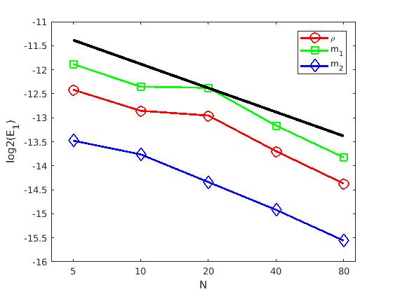
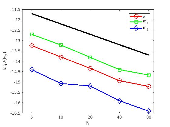
Figure 1: The statistical errors $E_{1}$ (left) and $E_{2}$(right) computed by the Monte Carlo VFV method on the mesh with $128\times 128$ cells. The black solid lines without any marker denote the reference slope of $N^{-1/2}$.

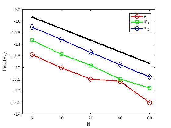
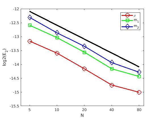
Figure 2: The statistical errors $E_{1}$ (left) and $E_{2}$(right) computed by the Monte Carlo VFV method on the mesh with $512\times 512$ cells. The black solid lines without any marker denote the reference slope of $N^{-1/2}$.

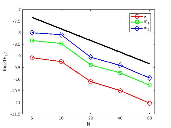
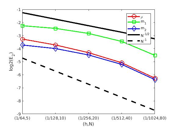
Figure 3: The statistical errors $E_{1}$ (left) and $E_{2}$(right) computed by the Monte Carlo VFV method on the mesh with $2048\times 2048$ cells. The black solid lines without any marker denote the reference slope of $N^{-1/2}$.

Table 3: The total error $E_{1}$ computed by the Monte Carlo VFV method with parameters $(h,N(h))$;  $h=1/(2^{\ell+5}),N(h)=5\cdot 2^{\ell-1},\ \ell=1,\dots,5.$

variables	$\varrho$		$m_{1}$		$m_{2}$
$(h,N(h))$	error	order	error	order	error	order
$(1/64,5)$	1.68e-01		4.29e-01		1.36e-01
$(1/128,10)$	1.14e-01	0.56	3.73e-01	0.20	1.10e-01	0.31
$(1/256,20)$	6.49e-02	0.81	2.76e-01	0.43	6.93e-02	0.67
$(1/512,40)$	3.24e-02	1.00	1.70e-01	0.70	3.50e-02	0.99
$(1/1024,80)$	1.23e-02	1.40	7.49e-02	1.18	1.33e-02	1.40

Table 4: The total error $E_{2}$ computed by the Monte Carlo VFV method with parameters $(h,N(h))$;  $h=1/(2^{\ell+5}),N(h)=5\cdot 2^{\ell-1},\ \ell=1,\dots,5.$

variables	$\varrho$		$m_{1}$		$m_{2}$
$(h,N(h))$	error	order	error	order	error	order
$(1/64,5)$	1.04e-01		2.11e-01		7.58e-02
$(1/128,10)$	7.60e-02	0.45	1.83e-01	0.21	6.28e-02	0.27
$(1/256,20)$	5.05e-02	0.59	1.40e-01	0.39	4.47e-02	0.49
$(1/512,40)$	2.96e-02	0.77	9.17e-02	0.61	2.71e-02	0.72
$(1/1024,80)$	1.31e-02	1.18	4.39e-02	1.06	1.21e-02	1.16

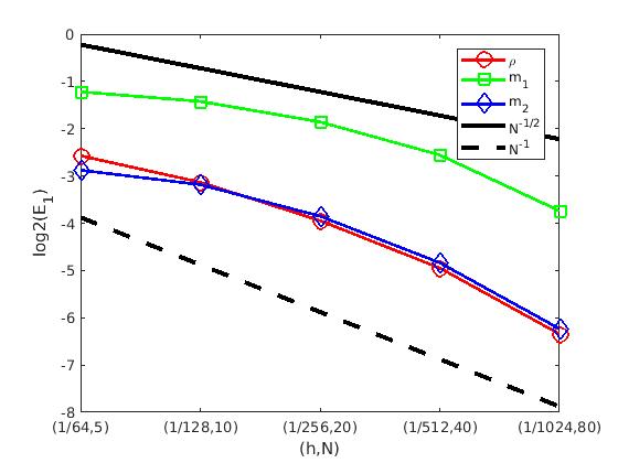
(a) $E_{1}$

(b) $E_{2}$

Figure 4: The errors $E_{1}$ and $E_{2}$ in $L^{1}-$norm with parmaters $h=1/(2^{\ell+5}),N(h)=5\cdot 2^{\ell-1},\ell=1,2,\dots,5.$ The black solid lines without any marker denote the reference slope of $N^{-1/2}$. The black dash lines without any marker denote the reference slope of $N^{-1}$.

Conclusions

In the present paper we have studied convergence of the Monte Carlo method combined with a consistent approximation for the random isentropic Euler equations. We work with the concept of dissipative weak solutions that can be seen as a universal closure of consistent approximations. Since the Euler equations are not uniquely solvable in the class of dissipative weak solutions we apply the set-valued version of the Strong law of large numbers for general multivalued mapping with closed range, cf. Theorem 4.2. For strong solutions this reduces to the strong convergence in $L^{q}((0,T)\times T^{d}),$ $q=\frac{2\gamma}{\gamma+1}.$ Combining Theorem 4.2 with the deterministic convergence results of a consistent approximation yield the convergence of the Monte Carlo method in the weak form, cf. Theorem 5.3. Applying $\mathcal{K}-$convergence in random setting we have derived the convergence of the Monte Carlo method in the strong form in Theorem 5.6. If the strong solution exists, we obtain the strong convergence of the Monte Carlo estimators obtained by the numerical approximation to the expected value of the unique strong statistical solution, cf. Theorem 6.1. In Section 7 we illustrate theoretical results by numerical simulations obtained by the Monte Carlo method combined with the viscosity finite volume method.

References

• [1] Z. Artstein and J. C. Hansen. Convexification in limit laws of random sets in Banach spaces. Ann. Probab., 13(1):307–309, 1985.
• [2] E. J. Balder. Lectures on Young measure theory and its applications in economics. Rend. Istit. Mat. Univ. Trieste, 31(suppl. 1):1–69, 2000. Workshop on Measure Theory and Real Analysis (Italian) (Grado, 1997).
• [3] E.J. Balder. On weak convergence implying strong convergence in $l^{1}$ spaces. Bull. Austral. Math. Soc., 33:363–368, 1986.
• [4] D. Breit, E. Feireisl, and M. Hofmanová. Solution semiflow to the isentropic Euler system. Arch. Ration. Mech. Anal., 235(1):167–194, 2020.
• [5] T. Buckmaster, C. de Lellis, L. Székelyhidi, Jr., and V. Vicol. Onsager’s conjecture for admissible weak solutions. Comm. Pure Appl. Math., 72(2):229–274, 2019.
• [6] T. Buckmaster and V. Vicol. Convex integration and phenomenologies in turbulence. EMS Surv. Math. Sci., 6(1):173–263, 2019.
• [7] R. M. Chen, A. F. Vasseur, and Ch. Yu. Global ill-posedness for a dense set of initial data to the isentropic system of gas dynamics. Adv. Math., 393:Paper No. 108057, 46, 2021.
• [8] E. Chiodaroli. A counterexample to well-posedness of entropy solutions to the compressible Euler system. J. Hyperbolic Differ. Equ., 11(3):493–519, 2014.
• [9] E. Chiodaroli, C. De Lellis, and O. Kreml. Global ill-posedness of the isentropic system of gas dynamics. Comm. Pure Appl. Math., 68(7):1157–1190, 2015.
• [10] E. Chiodaroli and E. Feireisl. On the density of ”wild” initial data for the barotropic Euler system. arxiv preprint No. 2208.04810, 2022.
• [11] E. Chiodaroli and E. Feireisl. Glimm’s method and density of wild data for the Euler system of gas dynamics. Nonlinearity, 37(3):Paper No. 035005, 12, 2024.
• [12] C. De Lellis and L. Székelyhidi, Jr. On admissibility criteria for weak solutions of the Euler equations. Arch. Ration. Mech. Anal., 195(1):225–260, 2010.
• [13] N. Etemadi. An elementary proof of the strong law of large numbers. Z. Wahrsch. Verw. Gebiete, 55(1):119–122, 1981.
• [14] E. Feireisl. A note on the long-time behavior of dissipative solutions to the Euler system. J. Evol. Equ., 21(3):2807–2814, 2021.
• [15] E. Feireisl. (S)-convergence and approximation of oscillatory solutions in fluid dynamics. Nonlinearity, 34(4):2327–2349, 2021.
• [16] E. Feireisl, S. S. Ghoshal, and A. Jana. On uniqueness of dissipative solutions to the isentropic Euler system. Comm. Partial Differential Equations, 44(12):1285–1298, 2019.
• [17] E. Feireisl and M. Hofmanová. On convergence of approximate solutions to the compressible Euler system. Ann. PDE, 6(2):11, 2020.
• [18] E. Feireisl, M. Lukáčová-Medvid’ová, B. She, and S. Schneider. Approximating viscosity solutions of the Euler system. Math. Comp., 91(337): 2129–2164, 2022.
• [19] E. Feireisl, M. Lukáčová-Medvid’ová, H. Mizerová, and B. She. Numerical Analysis of Compressible Fluid Flows. Springer-Verlag, Cham, 2022.
• [20] E. Feireisl and M. Lukáčová-Medvid’ová. Statistical solutions for the Navier–Stokes–Fourier system. Stoch PDE: Anal Comp, DOI:10.1007/s40072-023-00298-6, 2023.
• [21] E. Feireisl and M. Lukáčová-Medvid’ová, B. She, Y. Yuan. Convergence and error analysis of compressible fluid flows with random data: Monte Carlo method. Math. Models Methods Appl. Sci., 32(14):2887–2925, 2022.
• [22] E. Feireisl, M. Lukáčová-Medvid’ová, and H. Mizerová. $\mathcal{K}$-convergence as a new tool in numerical analysis. IMA J. Numer. Anal., 40(4):2227–2255, 2020.
• [23] E. Feireisl, M. Lukáčová-Medvid’ová, B. She, and Y. Wang. Computing oscillatory solutions of the Euler system via $\mathcal{K}$-convergence. Math. Mod.& Methods Appl. Sci., 31 (3): 537–576, 2021.
• [24] V. Giri and H. Kwon. On non-uniqueness of continuous entropy solutions to the isentropic compressible Euler equations. Arch. Ration. Mech. Anal., 245(2):1213–1283, 2022.
• [25] B. Guo and X. Wu. Qualitative analysis of solutions for the full compressible Euler equations in $\mathbb{R}^{N}$. Indiana Univ. Math. J., 67(1):343–373, 2018.
• [26] Ch. Hess. On multivalued martingales whose values may be unbounded: martingale selectors and Mosco convergence. J. Multivariate Anal., 39(1):175–201, 1991.
• [27] J. Komlós. A generalization of a problem of Steinhaus. Acta Math. Acad. Sci. Hungar., 18:217–229, 1967.
• [28] M. Lukáčová-Medvid’ová, B. She, Y. Yuan. Convergence analysis of the Monte Carlo method for the random Navier–Stokes–Fourier system, arxiv preprint No. 2304.00594, 2023.
• [29] A. Majda. Compressible Fluid Flow and Systems of Conservation Laws in Several Space Variables, volume 53 of Applied Mathematical Sciences. Springer-Verlag, New York, 1984.
• [30] J. Smoller. Shock Waves and Reaction-Diffusion Equations. Springer-Verlag, New York, 1967.
• [31] D. W. Stroock and S. R. S. Varadhan. Multidimensional Diffusion Processes. Classics in Mathematics. Springer-Verlag, Berlin, 2006. Reprint of the 1997 edition.
• [32] P. Terán. A multivalued strong law of large numbers. J. Theoret. Probab., 29(2):349–358, 2016.