Extinction and survival in inherited sterility

Abstract

We introduce an interacting particle system which models the inherited sterility method. Individuals evolve on $\mathbb{Z}^{d}$ according to a contact process with parameter $\lambda>0$. With probability $p\in[0,1]$ an offspring is fertile and can give birth to other individuals at rate $\lambda$. With probability $1-p$, an offspring is sterile and blocks the site it sits on until it dies. The goal is to prove that at fixed $\lambda$, the system survives for large enough $p$ and dies out for small enough $p$. The model is not attractive, since an increase of fertile individuals potentially causes that of sterile ones. However, thanks to a comparison argument with attractive models, we are able to answer our question.

Keywords: Interacting particle systems, Contact process, Coupling, Comparison Theorem.

1 Introduction

In this paper, we introduce an interacting particle system, suggested to us by Rinaldo Schinazi [16], to model the ”Inherited Sterility” (IS) method. This method, developed in the second half of the twentieth century, during the rise of intensive agriculture, is used in pest control management, in particular to fight against massive crop destruction by invasive species, see Inherited sterility in Lepidoptera [15]. The IS method is an adaptation of the Sterile Insect Technique (SIT), developed, among others, by E. Knipling in the 1950s to eradicate New World screw worms. In the SIT, the overall goal is to eradicate a population of insects through the use of a large number of males sterilized with gamma rays. They are released over infested areas to mate with fertile individuals, but give rise to no offspring, so the population eventually becomes extinct. However, for certain types of species such as Lepidoptera, a high level of radiation is needed to produce total infertility. This decreases the sexual competitiveness of sterilized individuals - as they carry with them a repulsive level of radiation - and therefore mitigates the effectiveness of the SIT. To counterbalance this effect, the species can be partially sterilized so that it produces a certain proportion of sterile offsprings, and another of fertile ones. The fertile offsprings themselves then have a certain chance of giving birth to fertile or sterile individuals and so on. This is what is called Inherited Sterility. We refer to the reference book [5] for a detailed list of trials and programs regarding the SIT and to Chapter 2.4 of the book for Inherited Sterility.

For a mathematical analysis of the SIT, an interacting particle system suggested by Rinaldo Schinazi is introduced in [10] as a toy model. At the microscopic level and in infinite volume, the author proves a phase transition result: depending on the choice of parameters for the system, the population survives or not. The macroscopic, out of equilibrium study of this particle system is investigated in [11] in infinite volume, and, more recently in [14], at equilibrium in finite volume with slow reservoirs. Another interacting particle system for the SIT is introduced in [8] where the study is done at the microscopic level, and where again the authors derive a phase transition result for survival or extinction of the population. Both in [10] and [8], the authors strongly rely on the monotonicity underlying the dynamics of the particle systems. This monotonicity property comes from the fact that the more fertile individuals are present, the more chances the population has of surviving. It turns out that for the IS technique, this is no longer the case. Indeed, having more fertile individuals at a certain time could imply having more sterile individuals at a later time, given that fertile individuals give rise to a proportion of sterile ones. This notable fact makes the mathematical analysis of an IS model quite challenging.

In our model, individuals evolve on $\mathbb{Z}^{d}$. They can either be fertile (in state $1$) or sterile (in state $-1$). Empty sites are said to be in state $0$. Furthermore, each site is occupied by at most one individual. Fertile individuals reproduce at a certain birth rate (or speed of reproduction) $\lambda>0$. There is a probability $p\in[0,1]$ that the offspring is born fertile and $1-p$ that it is born sterile. Our goal here is to investigate the microscopic behavior of the system when $\lambda>0$ is fixed and $p$ varies. In particular, we show that there is no monotonicity in $p$ in the system. Nonetheless, we manage to prove the following (see Theorem 1):

• There is a $\textbf{p}(\lambda)\in(0,1)$ such that for any $p\leq\textbf{p}(\lambda)$, the process with birth rate $\lambda$ and fertility probability $p$ becomes extinct (all the $1$’s die out).

• If $\lambda>0$ is large enough, there is a $\tilde{\textbf{p}}(\lambda)\in(0,1)$ such for any $p\geq\tilde{\textbf{p}}(\lambda)$, the process with birth rate $\lambda$ and fertility probability $p$ survives (there are infinitely often some $1$’s).

The strategy pursued is the following: to prove $(i)$ we show that our process is stochastically dominated by a basic contact process which becomes extinct when $p$ is small enough. To prove $(ii)$, we introduce a contact process with a dynamic random environment which survives when $\lambda$ and $p$ are large enough. We show that our process stochastically dominates it and therefore survives too. The difficulty relies on proving the survival of the contact process with dynamic random environment. For that, in the spirit of [9] and [10], we compare its graphical representation to oriented percolation, and use a renormalization argument. Our proof simplifies the strategy pursued in [9] and [10], as it weakens the hypothesis needed to apply the renormalization argument.

The paper is organized as follows. In Section 2, we introduce the models and state all the results. In Section 3 we define the graphical representation associated to each model and prove the stochastic dominations. In section 4, we prove the survival of the contact process with dynamic random environment.

2 Definitions and results

2.1 The inherited sterility model and main result

For $d\geq 1$, introduce the state space $\Omega=\{-1,0,1\}^{\mathbb{Z}^{d}}$, so that for $\eta\in\Omega$ and $x\in\mathbb{Z}^{d}$, $\eta(x)$ is the state of site $x$ in $\eta$. We say that

$$\eta(x)=\left\{\begin{array}[]{ll}1,\leavevmode\nobreak\ \leavevmode\nobreak\ \text{if there is a fertile individual at site }x,\\ -1,\leavevmode\nobreak\ \leavevmode\nobreak\ \text{if there is a sterile individual at site }x,\\ 0,\leavevmode\nobreak\ \leavevmode\nobreak\ \text{if site $x$ is empty}.\end{array}\right.$$ (2.1)

Two sites $x$ and $y$ are nearest neighbours in $\mathbb{Z}^{d}$ if $\|x-y\|_{1}=1$ and we write $x\sim y$.

Introduce $\eta_{1},\eta_{-1},\eta_{0}\in\{0,1\}^{\mathbb{Z}^{d}}$ as follows:

$$\eta_{1}(x)=\mathds{1}_{\eta(x)=1},\leavevmode\nobreak\ \leavevmode\nobreak\ \leavevmode\nobreak\ \eta_{-1}(x)=\mathds{1}_{\eta(x)=-1},\leavevmode\nobreak\ \leavevmode\nobreak\ \leavevmode\nobreak\ \eta_{0}(x)=\mathds{1}_{\eta(x)=0}.$$ (2.2)

For $x\in\mathbb{Z}^{d}$ and $\eta\in\Omega$, denote by $n_{1}(x,\eta)=\underset{y\sim x}{\sum}\eta_{1}(y)$ the number of neighbours of $x$ in state $1$ in $\eta$.

Definition 1.

The inherited sterility process with birth rate $\lambda>0$ and fertility probability $p\in[0,1]$, that we will refer to as $IS(\lambda,p)$, is the Markov jump process $(\eta_{t})_{t\geq 0}$ on the state space $\Omega$, whose transition rates at $x\in\mathbb{Z}^{d}$ for a current configuration $\eta$ are given by:

$$1,-1\rightarrow 0:\mathrm{at\leavevmode\nobreak\ rate\leavevmode\nobreak\ }1,\leavevmode\nobreak\ \leavevmode\nobreak\ 0\rightarrow 1:\mathrm{at\leavevmode\nobreak\ rate\leavevmode\nobreak\ }\lambda pn_{1}(x,\eta),\leavevmode\nobreak\ \leavevmode\nobreak\ 0\rightarrow-1:\mathrm{at\leavevmode\nobreak\ rate\leavevmode\nobreak\ }\lambda(1-p)n_{1}(x,\eta).$$ (2.3)

For $\eta\in\Omega$, $x\in\mathbb{Z}^{d}$ and $i\in\{-1,0,1\}$, denote by $\sigma^{i,x}\eta$ the configuration obtained from $\eta$ after flipping the state of $x$ to $i$:

$$\sigma^{i,x}\eta(y)=\left\{\begin{array}[]{ll}i,\leavevmode\nobreak\ \leavevmode\nobreak\ \text{if}\leavevmode\nobreak\ y=x\\ \eta(y),\leavevmode\nobreak\ \leavevmode\nobreak\ \text{otherwise}.\end{array}\right.$$ (2.4)

The infinitesimal generator of an $IS(\lambda,p)$ process is given by: for any cylinder function $f$ on $\Omega$ and configuration $\eta\in\Omega$,

$$\begin{split}\mathcal{L}f(\eta)&=\sum_{x\in\mathbb{Z}^{d}}\sum_{i\in\{-1,0,1\}}c(x,\eta,i)\big{[}f(\sigma^{i,x}\eta)-f(\eta)\big{]},\end{split}$$ (2.5)

with infinitesimal transition rates:

$$\begin{split}&c(x,\eta,1)=1,\leavevmode\nobreak\ \leavevmode\nobreak\ \leavevmode\nobreak\ \text{ if }\eta(x)\in\{-1,1\},\\ &c(x,\eta,1)=\lambda pn_{1}(x,\eta),\leavevmode\nobreak\ \leavevmode\nobreak\ \leavevmode\nobreak\ \text{ if }\eta(x)=0,\\ &c(x,\eta,-1)=\lambda(1-p)n_{1}(x,\eta),\leavevmode\nobreak\ \leavevmode\nobreak\ \leavevmode\nobreak\ \text{ if }\eta(x)=0.\end{split}$$ (2.6)

Since all the rates in (2.6) are bounded, by [12, Theorem 3.9], there exists a unique Markov process whose dynamics is induced by the infinitesimal generator (2.5).

For $\eta\in\Omega$, we will denote by $\mathbb{P}_{\eta}^{\lambda,p}$ the probability measure on the space of continuous time trajectories on $\Omega$ induced by $(\eta_{t})_{t\geq 0}$ when $\eta_{0}=\eta$. We also denote by

$$A(\eta)=\{x\in\mathbb{Z}^{d},\leavevmode\nobreak\ \eta(x)=1\}.$$ (2.7)

An $IS(\lambda,p)$ process $(\eta_{t})_{t\geq 0}$ is said to survive if,

$$\mathbb{P}_{\{0\}}^{\lambda,p}\Big{(}\forall t>0,\leavevmode\nobreak\ A(\eta_{t})\neq\emptyset\Big{)}>0,$$ (2.8)

where, by abuse of notation, $\{0\}$ is the configuration containing a $1$ at site $0$ and $0$’s everywhere else. The process is said to become extinct otherwise.

Theorem 1.

Fix $d\geq 1$ and $\lambda>0$:

• If $\lambda\leq\lambda_{c}(d)$, for any $p\in[0,1]$, an $IS(\lambda,p)$ process on $\mathbb{Z}^{d}$ almost surely becomes extinct.

• If $\lambda>\lambda_{c}(d)$, there exists a $\check{p}(\lambda)\in[\lambda_{c}(d)/\lambda,1)$ such that for any $p\geq\check{p}(\lambda)$, an $IS(\lambda,p)$ process on $\mathbb{Z}^{d}$ survives.

In the rest of the paper, if $X$ is a partially ordered set, given two configurations $\xi_{1}$ and $\xi_{2}$ in $X^{\mathbb{Z}^{d}}$, we say that $\xi_{1}\leq\xi_{2}$ if for any $x\in\mathbb{Z}^{d}$, $\xi_{1}(x)\leq\xi_{2}(x)$.

A convenient tool for the proof of extinction and survival in the context of non conservative particle systems is monotonicity, defined as follows:

Definition 2.

Consider $X$ a (partially) ordered set. A process $(\zeta_{t})_{t\geq 0}$ with values in $X^{\mathbb{Z}^{d}}$ and whose dynamics is parametrized by a certain value $q$ is said to be monotone in $q$ if, when $q_{1}\leq q_{2}$, one can couple $(\zeta^{(1)}_{t})_{t\geq 0}$ with dynamics parameter $q_{1}$, and $(\zeta^{(2)}_{t})_{t\geq 0}$ with dynamics parameter $q_{2}$, in such a way that

$$\zeta^{(1)}_{0}\leq\zeta^{(2)}_{0}\Rightarrow\zeta^{(1)}_{t}\leq\zeta^{(2)}_{t}\leavevmode\nobreak\ a.s.\leavevmode\nobreak\ \text{for all }t>0.$$

For our model, there is no monotonicity in $p$:

Proposition 1.

For any ordering of $\{-1,0,1\}$ and any $\lambda>0$, an $IS$ process on $\mathbb{Z}^{d}$ with birth rate $\lambda$ is not monotonous in the parameter $p$.

The proof of Proposition 1 is done in Section 3.

Remark 1.

It follows that in Theorem 1, one cannot rely on a monotonicity argument to prove that the phase transition in $p$ is sharp in the sense that: for $\lambda>\lambda_{c}(d)$, there is a critical parameter $p_{c}(\lambda)\in[\lambda_{c}(d)/\lambda,1)$ such that for any $p<p_{c}(\lambda)$, an $IS(\lambda,p)$ process becomes extinct and for any $p>p_{c}(\lambda)$, an $IS(\lambda,p)$ process survives.

2.2 Two other processes

The contact process

Recall that the contact process on $\mathbb{Z}^{d}$ with parameter $\lambda$ is an interacting particle system on the state space $\{0,1\}^{\mathbb{Z}^{d}}$, whose transition rates at $x$ for a current configuration $\zeta$ are given by:

$$0\rightarrow 1:\leavevmode\nobreak\ \text{at rate }\lambda n_{1}(x,\zeta),\leavevmode\nobreak\ \leavevmode\nobreak\ \text{and }1\rightarrow 0:\leavevmode\nobreak\ \text{at rate }1.$$ (2.9)

The contact process on $\mathbb{Z}^{d}$ exhibits a phase transition in the parameter $\lambda$ (we refer to [13, Part 1, section 2]) : there is a $\lambda_{c}(d)\in(0,\infty)$ such that for any $\lambda\leq\lambda_{c}(d)$, the contact process with parameter $\lambda$ almost surely reaches the empty configuration (extinction), and for $\lambda>\lambda_{c}(d)$, with strictly positive probability, the process never reaches the empty configuration (survival). We refer to [12] and [13] for detailed reviews on the contact process.

For $\eta\in\Omega$, we denote by $\textbf{P}_{\zeta}^{\lambda}$ the probability measure on the space of continuous time trajectories on $\Omega$ induced by $(\zeta_{t})_{t\geq 0}$, when $\zeta_{0}=\zeta$.

Remark 2.

Note that if $p=1$, an $IS(\lambda,p)$ process starting from a configuration in $\{0,1\}^{\mathbb{Z}^{d}}$ evolves according to a contact process on $\mathbb{Z}^{d}$ with parameter $\lambda$.

Theorem 2.

For any $(\lambda,p)\in(0,\infty)\times[0,1]$, and $(\eta_{0},\zeta_{0})\in\Omega\times\{0,1\}^{\mathbb{Z}^{d}}$ such that $\eta_{0}\leq\zeta_{0}$, there exists a coupling $(\eta_{t},\zeta_{t})_{t\geq 0}$, on $\Omega\times\{0,1\}^{\mathbb{Z}^{d}}$, such that $(\eta_{t})_{t\geq 0}$ is an $IS(\lambda,p)$ process starting from $\eta_{0}$, $(\zeta_{t})_{t\geq 0}$ a contact process with birth rate $\lambda p$ starting from $\zeta_{0}$, and satisfying:

$$\eta_{t}\leq\zeta_{t}\leavevmode\nobreak\ \leavevmode\nobreak\ \leavevmode\nobreak\ \leavevmode\nobreak\ \leavevmode\nobreak\ \text{a.s.}\leavevmode\nobreak\ \leavevmode\nobreak\ \leavevmode\nobreak\ \leavevmode\nobreak\ \forall t\geq 0.$$

The proof of Theorem 2 is done using the basic coupling on the graphical representation and we refer to Section 3.2 for more details.

A contact process with dynamic random environment

Definition 3.

For $\lambda>0$ and $p\in[0,1]$, the $Spont(\lambda,p)$ process is the Markovian jump process $(\xi_{t})_{t\geq 0}$ on the state space $\Omega$ whose transition rates at site $x\in\mathbb{Z}^{d}$ for a current configuration $\xi$ are given by:

$$0\rightarrow 1:\leavevmode\nobreak\ \mathrm{at\leavevmode\nobreak\ rate\leavevmode\nobreak\ }\lambda pn_{1}(x,\xi),\leavevmode\nobreak\ \leavevmode\nobreak\ 0\rightarrow-1:\leavevmode\nobreak\ \mathrm{at\leavevmode\nobreak\ rate\leavevmode\nobreak\ }2d\lambda(1-p)\leavevmode\nobreak\ \leavevmode\nobreak\ \mathrm{and}\leavevmode\nobreak\ \leavevmode\nobreak\ 1,-1\rightarrow 0:\leavevmode\nobreak\ \mathrm{at\leavevmode\nobreak\ rate\leavevmode\nobreak\ }1.$$ (2.10)

In other words, the dynamics is that of a contact process with parameter $\lambda p$, where empty sites become randomly blocked, i.e., no sites in state $1$ can reproduce on neighbouring blocked sites before they flip back to $0$.

The infinitesimal generator of a $Spont(\lambda,p)$ process is given by: for any cylinder function $f$ on $\Omega$ and configuration $\xi\in\Omega$,

$$\begin{split}\mathbb{L}f(\xi)&=\sum_{x\in\mathbb{Z}^{d}}\sum_{i\in\{-1,0,1\}}c_{spont}(x,\xi,i)\big{[}f(\sigma^{i,x}\xi)-f(\xi)\big{]},\end{split}$$ (2.11)

with infinitesimal transition rates:

$$\begin{split}&c_{spont}(x,\xi,1)=1,\text{ if }\xi(x)\in\{-1,1\},\\ &c_{spont}(x,\xi,1)=\lambda pn_{1}(x,\xi),\text{ if }\xi(x)=0,\\ &c_{spont}(x,\xi,-1)=2d\lambda(1-p),\text{ if }\xi(x)=0.\end{split}$$ (2.12)

Since all the rates in (2.12) are bounded, by [12, Theorem 3.9] there exists a unique Markov process whose dynamics is induced by the infinitesimal generator (2.11).

For $\xi\in\Omega$, we will denote by $\tilde{\mathbb{P}}_{\xi}^{\lambda,p}$ the probability measure on the space of continuous time trajectories on $\Omega$ induced by $(\eta_{t})_{t\geq 0}$, when $\xi_{0}=\xi$.

The following result tells us that a $Spont(\lambda,p)$ process is stochatically dominated by an $IS(\lambda,p)$ process:

Theorem 3.

For any $(\lambda,p)\in(0,\infty)\times[0,1]$, and $(\xi_{0},\eta_{0})\in\Omega^{2}$ such that $\eta_{0}\leq\zeta_{0}$, there exists a coupling $(\xi_{t},\eta_{t})_{t\geq 0}$, on $\Omega^{2}$ such that $(\xi_{t})_{t\geq 0}$ is an $Spont(\lambda,p)$ process starting from $\xi_{0}$, $(\eta_{t})_{t\geq 0}$ an $IS(\lambda,p)$ process starting from $\eta_{0}$ and satisfying :

$$\xi_{t}\leq\eta_{t}\leavevmode\nobreak\ \leavevmode\nobreak\ \leavevmode\nobreak\ \leavevmode\nobreak\ \leavevmode\nobreak\ \text{a.s.}\leavevmode\nobreak\ \leavevmode\nobreak\ \leavevmode\nobreak\ \leavevmode\nobreak\ \forall t\geq 0.$$

The proof of Theorem 3 is done using the basic coupling on the graphical representation and we refer to Section 3.2 for more details.

The $Spont$ process satisfies the following:

Theorem 4.

Phase transition for the $Spont$ process.

Fix $\lambda>\lambda_{c}(d)$. The $Spont$ process with birth rate $\lambda$ exhibits a non trivial phase transition in the parameter $p$: there exists $p_{c}^{spont}(\lambda)\in[\lambda_{c}(d)/\lambda,1)$, such that

• For any $p<p_{c}^{spont}(\lambda)$, the process $Spont(\lambda,p)$ becomes extinct.

• For any $p>p_{c}^{spont}(\lambda)$, the process $Spont(\lambda,p)$ survives.

The proof of Theorem 4 is postponed to Section 4 and relies on the fact that for $Spont$, contrary to $IS$, monotonicity holds.

2.3 Proof of Theorem 1

Collecting the results stated in Section 2.2, we are in position to prove Theorem 1.

• By Theorem 2, we can consider a coupling $(\eta_{t},\zeta_{t})$ between an $IS(\lambda,p)$ process and a contact process with parameter $\lambda p$, both starting from the configuration $\{0\}$, such that

  $$A(\eta_{t})\subset A(\zeta_{t})\leavevmode\nobreak\ \leavevmode\nobreak\ \leavevmode\nobreak\ a.s.\leavevmode\nobreak\ \leavevmode\nobreak\ \leavevmode\nobreak\ \forall t\geq 0.$$

  Therefore,

  $$\mathbb{P}_{\{0\}}^{\lambda,p}\Big{(}\forall t,\leavevmode\nobreak\ A(\eta_{t})\neq\emptyset\Big{)}\leq\textbf{P}_{\{0\}}^{\lambda p}\Big{(}\forall t,\leavevmode\nobreak\ A(\zeta_{t})\neq\emptyset\Big{)}.$$ (2.13)

  It follows that for $p\leq\lambda_{c}(d)/\lambda$, a contact process with parameter $\lambda p$ becomes extinct so the upper bound in (2.13) is zero. Hence, the $IS(\lambda,p)$ process become extinct. In particular, this holds for any $p\in[0,1]$, as soon as $\lambda\leq\lambda_{c}(d)$.

• As just seen, for $\lambda\leq\lambda_{c}$, for any $p\in[0,1]$, an $IS(\lambda,p)$ process become extinct. Fix $\lambda>\lambda_{c}$. By Theorem 3 we can consider a coupling $(\xi_{t},\eta_{t})$ between a $Spont(\lambda,p)$ process and an $IS(\lambda,p)$ both starting from the configuration $\{0\}$, such that

  $$A(\xi_{t})\subset A(\eta_{t})\leavevmode\nobreak\ \leavevmode\nobreak\ \leavevmode\nobreak\ a.s.\leavevmode\nobreak\ \leavevmode\nobreak\ \leavevmode\nobreak\ \forall t\geq 0.$$

  Therefore,

  $$\tilde{\mathbb{P}}_{\{0\}}^{\lambda,p}\Big{(}\forall t,\leavevmode\nobreak\ A(\xi_{t})\neq\emptyset\Big{)}\leq\mathbb{P}_{\{0\}}^{\lambda,p}\Big{(}\forall t,\leavevmode\nobreak\ A(\eta_{t})\neq\emptyset\Big{)}.$$

  By Theorem 4, for $p>p_{c}^{spont}(\lambda)$, the process $Spont(\lambda,p)$ survives so the lower bound in ((ii)) is strictly positive. It turns out that for any $p>p_{c}^{spont}(\lambda)$ the $IS(\lambda,p)$ process survives and $p_{c}(\lambda)\in[\lambda_{c}(d)/\lambda,1)$. Taking $\check{p}(\lambda)=p_{c}(\lambda)$, the result follows.

3 Graphical representations and couplings

The processes introduced in Section 2 can be alternatively described by a graphical representation, which gives another way of defining their dynamics, through the use of Poisson point processes. This construction was introduced by Harris, see [7]. The advantage of the graphical representation is that it allows to build very natural couplings between processes, and in particular, to prove some monotonicity properties. It also allows to compare the evolution of the set of occupied sites to that of a percolation cluster on an oriented percolation graph. This key feature will be central in the following Section.

3.1 Graphical representations

Fix $\lambda>0$ and $p\in[0,1]$. Consider the diagram $\mathbb{Z}^{d}\times\mathbb{R}_{+}$. Denote by $E(\mathbb{Z}^{d})$ the set of oriented edges of $\mathbb{Z}^{d}$. To each element $(x,y)\in E(\mathbb{Z}^{d})$ we associate the realization of a Poisson point process $(N_{1}^{x,y})_{(x,y)\in\mathbb{Z}^{d}}$ of parameter $\lambda p$, as well as that of a Poisson point process $(N_{2}^{x,y})_{(x,y)\in\mathbb{Z}^{d}}$ of parameter $\lambda(1-p).$ Also, consider two families of realizations of Poisson point processes $(U_{x})_{x\in\mathbb{Z}^{d}}$ and $(V_{x})_{x\in\mathbb{Z}^{d}}$ with rate $1$. We suppose that all these Poisson processes are sampled independently. From them, one can build the $IS(\lambda,p)$ process, the $Spont(\lambda,p)$ process and the contact process with parameter $\lambda$ as follows:

• For $IS(\lambda,p)$: at each time event $t$ of $N_{1}^{x,y}$, draw an arrow $\overset{1}{\longrightarrow}$ in $\mathbb{Z}^{d}\times\mathbb{R}_{+}$ from $(x,t)$ to $(y,t)$ to indicate that if $x$ is in state $1$ and $y$ in state $0$, the birth of a fertile individual occurs in $y$ (it flips to state $1$, see blue arrows in Figure 1). At each time event $t$ of $N_{2}^{x,y}$, draw an arrow $\overset{-1}{\longrightarrow}$ in $\mathbb{Z}^{d}\times\mathbb{R}_{+}$ from $(x,t)$ to $(y,t)$ to indicate that if $x$ is in state $1$ and $y$ in state $0$, the birth of a sterile individual occurs in $y$ (it flips to state $-1$, see red arrows in Figure 1). For each time event $t$ of $U_{x}$, resp. $V_{x}$ , place a symbol $\times$ (black cross in Figure 1), resp. $o$ (red dot in Figure 1) at $(x,t)$ to indicate that if $x$ was in state $1$ resp. $-1$, it flips to zero.

• For $Spont(\lambda,p)$: perform the same steps as for the graphical representation of $IS(\lambda,p)$ except that at each time event $t$ of $N_{2}^{x,y}$, draw an arrow $\overset{-1}{\longrightarrow}$ in $\mathbb{Z}^{d}\times\mathbb{R}_{+}$ from $(x,t)$ to $(y,t)$ to indicate that if $y$ is in state $0$, it flips to state $-1$, regardless of the state of $x$.

• For the contact process with parameter $\lambda p$: perform the same steps as for the graphical representation of $IS(\lambda,p)$ and ignore the effects of the Poisson point processes $(N^{2}_{x,y})_{(x,y)\in E(\mathbb{Z}^{d})}$ and $(V_{x})_{x\in\mathbb{Z}^{d}}$.

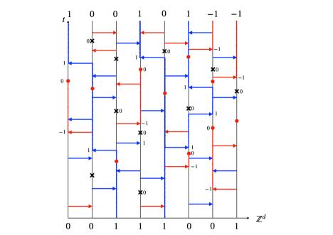
Figure 1: Graphical representation for a one dimensional $IS$ process. The blue, resp. red arrows, correspond to births of fertile, resp. sterile individuals. The black crosses, resp. red dots, correspond to deaths of fertile, resp. sterile individuals. The blue paths correspond to space-time active paths along which individuals survive. The red segments correspond to blocked sites due to the presence of a sterile individual, that is, sites where fertile individuals cannot be born, until the sterile individual blocking the site dies.

Given a graphical representation, an active path refers to a connected oriented path, moving along the time lines in the increasing direction of time and passing along arrows $\overset{1}{\longrightarrow}$, which crosses neither symbols $\times$ nor space-time points that are in state $-1$. Then, an $IS(\lambda,p)$, resp. $Spont(\lambda,p)$, resp. contact process starting from a configuration $\eta$, resp. $\xi$, resp. $\zeta$, can be built from the percolation structure described above, following the indications given by the different space time events. In particular, if the process starts with $1$’s in a given set $\mathcal{A}(\eta)$, resp. $\mathcal{A}(\xi)$, resp. $\mathcal{A}(\zeta)$, and $0$’s everywhere else, the set of $1$’s at time $t$ in $(\eta_{t})_{t\geq 0}$, resp. $(\xi_{t})_{t\geq 0}$, resp. $(\zeta_{t})_{t\geq 0}$ is given by:

$$\mathcal{A}_{t}(\eta)=\Big{\{}y\in\mathbb{Z}^{d},\leavevmode\nobreak\ \exists x\in\mathcal{A}(\eta)\leavevmode\nobreak\ \text{such that there is an active path from}\leavevmode\nobreak\ (x,0)\leavevmode\nobreak\ \text{to}\leavevmode\nobreak\ \leavevmode\nobreak\ (y,t)\Big{\}},$$

$$\text{resp. }\mathcal{A}_{t}(\xi)=\Big{\{}y\in\mathbb{Z}^{d},\leavevmode\nobreak\ \exists x\in\mathcal{A}(\xi)\leavevmode\nobreak\ \text{such that there is an active path from}\leavevmode\nobreak\ (x,0)\leavevmode\nobreak\ \text{to}\leavevmode\nobreak\ \leavevmode\nobreak\ (y,t)\Big{\}},$$

$$\text{resp. }\mathcal{A}_{t}(\zeta)=\Big{\{}y\in\mathbb{Z}^{d},\leavevmode\nobreak\ \exists x\in\mathcal{A}(\zeta)\leavevmode\nobreak\ \text{such that there is an active path from}\leavevmode\nobreak\ (x,0)\leavevmode\nobreak\ \text{to}\leavevmode\nobreak\ \leavevmode\nobreak\ (y,t)\Big{\}}.$$

We refer to [4, Section 2] for a proof that the graphical construction in the case of the contact process is well defined, and it adapts here for the graphical construction of the $IS(\lambda,p)$ process. We refer to [7] to check that the dynamics thus defined by the graphical representation matches the one in Definition 1.

3.2 Couplings

The graphical representations of processes allow to build the so called basic couplings. They essentially consist in using some common Poisson Processes in their graphical representation. We use these coupling to prove Theorems 2 and 3.

Proof of Theorem 2.

Take $\lambda>0$ and $p\in[0,1]$. Consider two configurations $(\eta,\zeta)\in\Omega\times\{0,1\}^{\mathbb{Z}^{d}}$ such that $\eta\leq\zeta$. Sample independent families of Poisson point processes $(N^{1}_{x,y})_{(x,y)\in E(\mathbb{Z}^{d})}$, $(N^{2}_{x,y})_{(x,y)\in E(\mathbb{Z}^{d})}$, $(U_{x})_{x\in\mathbb{Z}^{d}}$, $(V_{x})_{x\in\mathbb{Z}^{d}}$ with respective parameters $\lambda p$, $\lambda(1-p)$ and $1$. Deduce the evolution of an $IS(\lambda,p)$ process $(\eta_{t})_{t\geq 0}$ starting from $\eta_{0}$, and that of a contact process $(\zeta_{t})_{t\geq 0}$ with parameter $\lambda p$ starting from $\zeta_{0}$, by using their graphical representation and using the same Poisson point processes for that.

When a site $x\in\mathbb{Z}^{d}$ flips from $0$ to $1$ in $(\eta_{t})_{t\geq 0}$, so does this happen for $(\zeta_{t})_{t\geq 0}$, if $x$ was in state $0$ in $(\zeta_{t})_{t\geq 0}$. Indeed, for such a flip to happen at $s>0$, there must be a $y\sim x$, such that an arrow $\overset{1}{\longrightarrow}$ is produced by $N^{1}_{y,x}$ for the graphical construction of $IS(\lambda,p)$, and such that $\eta_{s^{-}}(y)=1$. This implies that $\zeta_{s^{-}}(y)=1$, so the arrow $\overset{1}{\longrightarrow}$ is also produced by $N^{1}_{y,x}$ for the graphical construction of the contact process with parameter $\lambda p$. Thus, $x$ flips from $0$ to $1$ in $(\zeta_{t})_{t\geq 0}$. Furthermore, as we use the same Poisson point processes $(V_{x})_{x\in\mathbb{Z}^{d}}$ for the flippings of $1$ to $0$, such flips in $(\zeta_{t})_{t\geq 0}$ happen simultaneously in $(\eta_{t})_{t\geq 0}$. Therefore, flips from $0$ to $1$ in $(\eta_{t})_{t\geq 0}$ and flips from $1$ to $0$ in $\zeta_{t}$ can never disrupt the order, so the basic coupling is order preserving.

In terms of transition rates, the basic coupling between $IS(\lambda,p)$ and the contact process with parameter $\lambda$ goes as follows. At site $x\in\mathbb{Z}^{d}$, for a current configuration $(\eta,\zeta)$:

$$\begin{split}&(1,1)\rightarrow(0,0):1,\leavevmode\nobreak\ \leavevmode\nobreak\ \leavevmode\nobreak\ \leavevmode\nobreak\ \leavevmode\nobreak\ \leavevmode\nobreak\ \leavevmode\nobreak\ \leavevmode\nobreak\ \leavevmode\nobreak\ \leavevmode\nobreak\ \leavevmode\nobreak\ \leavevmode\nobreak\ \leavevmode\nobreak\ \leavevmode\nobreak\ \leavevmode\nobreak\ \leavevmode\nobreak\ \leavevmode\nobreak\ \leavevmode\nobreak\ \leavevmode\nobreak\ \leavevmode\nobreak\ \leavevmode\nobreak\ (0,1)\rightarrow\left\{\begin{array}[]{ll}(0,0):\leavevmode\nobreak\ 1\\ (1,1):\leavevmode\nobreak\ \lambda pn_{1}(x,\eta)\\ (-1,1):\leavevmode\nobreak\ \lambda(1-p)n_{1}(x,\eta)\end{array}\right.,\\ \\ &(0,0)\rightarrow\left\{\begin{array}[]{ll}(1,1):\leavevmode\nobreak\ \lambda pn_{1}(x,\eta)\\ (0,1):\leavevmode\nobreak\ \lambda pn_{1}(x,\zeta)-\lambda pn_{1}(x,\eta)\\ (-1,0):\leavevmode\nobreak\ \lambda(1-p)n_{1}(x,\eta)\end{array}\right.,\leavevmode\nobreak\ \leavevmode\nobreak\ \leavevmode\nobreak\ (-1,1)\rightarrow\left\{\begin{array}[]{ll}(0,1):\leavevmode\nobreak\ 1\\ (-1,0):\leavevmode\nobreak\ 1\end{array}\right.,\\ \\ &(-1,0)\rightarrow\left\{\begin{array}[]{ll}(-1,1):\leavevmode\nobreak\ \lambda pn_{1}(x,\zeta)\\ (0,0):\leavevmode\nobreak\ 1\end{array}\right.,\end{split}$$ (3.1)

where we recall that $n_{1}(x,\eta)$, resp. $n_{1}(x,\zeta)$, is the number of neighbours of $x$ in state $1$ in $\eta$, resp. $\zeta$. Since $\eta\leq\zeta$, the rates are positive and the transition rates are well defined. ∎

Proof of Theorem 2.

Take $\lambda>0$ and $p\in[0,1]$. Consider two configurations $(\eta_{0},\xi_{0})\in\Omega^{2}$ such that $\xi_{0}\leq\eta_{0}$. As in the previous proof, sample independent families of Poisson point processes $(N^{1}_{x,y})_{(x,y)\in E(\mathbb{Z}^{d})}$, $(N^{2}_{x,y})_{(x,y)\in E(\mathbb{Z}^{2})}$, $(U_{x})_{x\in\mathbb{Z}^{d}}$, $(V_{x})_{x\in\mathbb{Z}^{d}}$ with respective parameters $\lambda p$, $\lambda(1-p)$ and $1$. Deduce the evolution of an $IS(\lambda,p)$ process $(\eta_{t})_{t\geq 0}$ starting from $\eta_{0}$, and that of a $Spont(\lambda,p)$ process $(\xi_{t})_{t\geq 0}$ starting from $\xi_{0}$, by using their graphical representation and using the same Poisson point processes for that.

When a site $x\in\mathbb{Z}^{d}$ flips from $0$ to $1$ in $(\xi_{t})_{t\geq 0}$, so does this happen for $(\eta_{t})_{t\geq 0}$, if $x$ was in state $0$, as this happens under the effect of the same arrows $\overset{1}{\longrightarrow}$ produced by $N^{1}_{y,x}$. Furthermore, when a site $x\in\mathbb{Z}^{d}$ flips from $0$ to $-1$ in $(\zeta_{t})_{t\geq 0}$, so does this happen for $(\xi_{t})_{t\geq 0}$, if $x$ was in state $0$. Indeed, for such a flip to happen at $s>0$, there must be a $y\sim x$ such that an arrow $\overset{-1}{\longrightarrow}$ is produced by $N^{2}_{y,x}$ for the graphical construction of $IS(\lambda,p)$, but this arrow is activated for $(\xi_{t})_{t\geq 0}$ at $s$, whatever the state of $y$. Finally, as we use the same processes $(U_{x})_{x\in\mathbb{Z}^{d}}$, resp. $(V_{x})_{x\in\mathbb{Z}^{d}}$, for the flippings of $1$ to $0$, resp. $-1$ to $0$ in $\eta$ and $\xi$, such flips happen simultaneously. Therefore, flips from $0$ to $1$ in $(\xi_{t})_{t\geq 0}$, from $1$ to $0$ in $(\zeta_{t})_{t\geq 0}$, from $0$ to $-1$ in $(\eta_{t})_{t\geq 0}$ and from $-1$ to $0$ in $(\xi_{t})_{t\geq 0}$, can never disrupt the order, so the basic coupling is order preserving.

In terms of transition rates, the basic coupling between $IS(\lambda,p)$ and a $Spont(\lambda,p)$ process goes as follows. At site $x\in\mathbb{Z}^{d}$, for a current configuration $(\eta,\zeta)$:

$$\begin{split}&(0,0)\rightarrow\left\{\begin{array}[]{ll}(1,1):\leavevmode\nobreak\ \lambda pn_{1}(x,\xi)\\ \\ (0,1):\leavevmode\nobreak\ \lambda p\big{[}n_{1}(x,\eta)-n_{1}(x,\xi)\big{]}\\ \\ (-1,-1):\leavevmode\nobreak\ \lambda(1-p)n_{1}(x,\eta)\\ \\ (-1,0):\leavevmode\nobreak\ \lambda(1-p)\big{[}2d-n_{1}(x,\eta)\big{]}\end{array}\right.,\leavevmode\nobreak\ \leavevmode\nobreak\ \leavevmode\nobreak\ \leavevmode\nobreak\ (0,1)\rightarrow\left\{\begin{array}[]{ll}(0,0):\leavevmode\nobreak\ 1\\ \\ (-1,1):\leavevmode\nobreak\ 2d\lambda(1-p)\\ \\ (1,1):\leavevmode\nobreak\ \lambda pn_{1}(x,\xi)\end{array}\right.,\\ \\ &(-1,1)\rightarrow\left\{\begin{array}[]{ll}(-1,0):\leavevmode\nobreak\ 1\\ \\ (0,1):\leavevmode\nobreak\ 1\end{array}\right.\leavevmode\nobreak\ \leavevmode\nobreak\ ,\leavevmode\nobreak\ \leavevmode\nobreak\ \leavevmode\nobreak\ \leavevmode\nobreak\ \leavevmode\nobreak\ \leavevmode\nobreak\ \leavevmode\nobreak\ \leavevmode\nobreak\ \leavevmode\nobreak\ \leavevmode\nobreak\ \leavevmode\nobreak\ \leavevmode\nobreak\ \leavevmode\nobreak\ \leavevmode\nobreak\ \leavevmode\nobreak\ \leavevmode\nobreak\ \leavevmode\nobreak\ \leavevmode\nobreak\ \leavevmode\nobreak\ \leavevmode\nobreak\ \leavevmode\nobreak\ \leavevmode\nobreak\ \leavevmode\nobreak\ \leavevmode\nobreak\ \leavevmode\nobreak\ \leavevmode\nobreak\ \leavevmode\nobreak\ \leavevmode\nobreak\ \leavevmode\nobreak\ (-1,-1)\rightarrow(0,0):1\\ \\ &(-1,0)\rightarrow\left\{\begin{array}[]{ll}(0,0):\leavevmode\nobreak\ 1\\ \\ (-1,1):\leavevmode\nobreak\ \lambda pn_{1}(x,\eta)\\ \\ (-1,-1):\leavevmode\nobreak\ \lambda(1-p)n_{1}(x,\eta)\end{array}\right.,\leavevmode\nobreak\ \mathrm{and}\leavevmode\nobreak\ \leavevmode\nobreak\ \leavevmode\nobreak\ \leavevmode\nobreak\ \leavevmode\nobreak\ \leavevmode\nobreak\ \leavevmode\nobreak\ \leavevmode\nobreak\ \leavevmode\nobreak\ \leavevmode\nobreak\ \leavevmode\nobreak\ \leavevmode\nobreak\ (1,1)\rightarrow(0,0):1.\end{split}$$ (3.2)

Since $\xi_{0}\leq\eta_{0}$, the rates are positive and the dynamics is well defined. One can check that $(\xi_{t})_{t\geq 0}$ is a $Spont(\lambda,p)$ process on $\mathbb{Z}^{d}$ and $(\eta_{t})_{t\geq 0}$ is an $IS(\lambda,p)$ process with parameter $\lambda p$ and that almost surely, for any $t\geq 0$, $\xi_{t}\leq\eta_{t}$.

∎

3.3 Monotonicity for $Spont(\lambda,p)$, lack of monotonicity for $IS(\lambda,p)$

Contrary to $IS$ processes (see Proposition 1 and its proof in this subsection), we have monotonicity in $p$ at fixed $\lambda$ for $Spont$ processes:

Proposition 2.

Fix $\lambda>0$ and $p_{1}<p_{2}$ in $[0,1]$. There exists a coupling $(\xi_{t}^{(1)},\xi_{t}^{(2)})_{t\geq 0}$ on $\Omega^{2}$ such that $(\xi_{t}^{(1)})_{t\geq 0}$, resp. $(\xi_{t}^{(2)})_{t\geq 0}$ is a $Spont(\lambda,p_{1})$, resp. $Spont(\lambda,p_{2})$ process and

$$\xi_{0}^{(1)}\leq\xi_{0}^{(2)}\Rightarrow\leavevmode\nobreak\ \leavevmode\nobreak\ \leavevmode\nobreak\ \xi_{t}^{(1)}\leq\xi_{t}^{(2)}\leavevmode\nobreak\ \leavevmode\nobreak\ a.s.\leavevmode\nobreak\ \text{for all }t\geq 0.$$ (3.3)

Proof.

Again, the basic coupling provides an order preserving coupling. For that, consider Poisson point processes indexed by oriented edges and sites $N^{1}_{x,y}$, $\tilde{N}^{1}_{x,y}$, $N^{2}_{x,y}$, $\tilde{N}^{2}_{x,y}$, $U_{x}$, $V_{x}$, with respective parameters $\lambda p_{1}$, $\lambda(p_{2}-p_{1})$, $2d\lambda(1-p_{2})$, $2d\lambda(p_{2}-p_{1})$, $1$ and $1$. Then, build the graphical representation for $Spont(\lambda,p_{1})$ by using $N^{1}_{x,y}$, $N^{2}_{x,y}+\tilde{N}^{2}_{x,y}$, $U_{x}$ and $V_{x}$, and the graphical representation for $Spont(\lambda,p_{2})$ by using $N^{1}_{x,y}+\tilde{N}^{2}_{x,y}$, $N^{2}_{x,y}$, $U_{x}$ and $V_{x}$. As in the proofs in Section 3.2, one can check that this coupled graphical representation is order preserving.

The rates of this coupling are given as follows. At site $x\in\mathbb{Z}^{d}$ for a current couple of configuration $(\xi,\tilde{\xi})$:

$$\begin{split}&(0,0)\rightarrow\left\{\begin{array}[]{ll}(1,1):\leavevmode\nobreak\ \lambda pn_{1}(x,\xi)\\ \\ (0,1):\leavevmode\nobreak\ \lambda p_{2}n_{1}(x,\tilde{\xi})-\lambda p_{1}n_{1}(x,\xi)\\ \\ (-1,-1):\leavevmode\nobreak\ 2d\lambda(1-p_{2})\\ \\ (-1,0):\leavevmode\nobreak\ 2d\lambda(p_{2}-p_{1})\end{array}\right.,\leavevmode\nobreak\ \leavevmode\nobreak\ \leavevmode\nobreak\ \leavevmode\nobreak\ (0,1)\rightarrow\left\{\begin{array}[]{ll}(0,0):\leavevmode\nobreak\ 1\\ \\ (-1,1):\leavevmode\nobreak\ 2d\lambda(1-p_{1})\\ \\ (1,1):\leavevmode\nobreak\ \lambda p_{1}n_{1}(x,\xi)\end{array}\right.,\\ \\ &(-1,1)\rightarrow\left\{\begin{array}[]{ll}(-1,0):\leavevmode\nobreak\ 1\\ \\ (0,1):\leavevmode\nobreak\ 1.\end{array}\right.\leavevmode\nobreak\ \leavevmode\nobreak\ ,\leavevmode\nobreak\ \leavevmode\nobreak\ \leavevmode\nobreak\ \leavevmode\nobreak\ \leavevmode\nobreak\ \leavevmode\nobreak\ \leavevmode\nobreak\ \leavevmode\nobreak\ \leavevmode\nobreak\ \leavevmode\nobreak\ \leavevmode\nobreak\ \leavevmode\nobreak\ \leavevmode\nobreak\ \leavevmode\nobreak\ \leavevmode\nobreak\ \leavevmode\nobreak\ \leavevmode\nobreak\ \leavevmode\nobreak\ \leavevmode\nobreak\ \leavevmode\nobreak\ \leavevmode\nobreak\ \leavevmode\nobreak\ \leavevmode\nobreak\ \leavevmode\nobreak\ \leavevmode\nobreak\ \leavevmode\nobreak\ \leavevmode\nobreak\ \leavevmode\nobreak\ \leavevmode\nobreak\ (-1,-1)\rightarrow(0,0):1\\ \\ &(-1,0)\rightarrow\left\{\begin{array}[]{ll}(0,0):\leavevmode\nobreak\ 1\\ \\ (-1,1):\leavevmode\nobreak\ \lambda p_{2}n_{1}(x,\tilde{\xi})\\ \\ (-1,-1):\leavevmode\nobreak\ 2d\lambda(1-p_{1})\end{array}\right.,\leavevmode\nobreak\ \mathrm{and}\leavevmode\nobreak\ \leavevmode\nobreak\ \leavevmode\nobreak\ \leavevmode\nobreak\ \leavevmode\nobreak\ \leavevmode\nobreak\ \leavevmode\nobreak\ \leavevmode\nobreak\ \leavevmode\nobreak\ \leavevmode\nobreak\ \leavevmode\nobreak\ \leavevmode\nobreak\ (1,1)\rightarrow(0,0):1.\end{split}$$ (3.4)

∎

Now let us prove Proposition 1, which claims that for any ordering of $\{-1,0,1\}$, there is no monotonicity in $p$ for an $IS$ process at fixed $\lambda$. First note that the basic coupling, built as in the proof of Proposition 2, does not provide an order preserving coupling, whatever the order on $\{-1,0,1\}$. In fact, hereafter we only consider orders where $1$ is the maximal element of the set, as we are interested in the survival of $1$’s.

• For the order $-1<0<1$: consider $\eta^{1},\eta^{2}\in\Omega^{2}$ with $\eta^{1}\leq\eta^{2}$, such that there is $x\sim y\in\mathbb{Z}^{d}$ with $\eta^{1}(x)=\eta^{1}(y)=0$, $\eta^{2}(x)=1$ and $\eta^{2}(y)=0$. If an arrow $\overset{-1}{\longrightarrow}$ is produced by $N^{2}_{x,y}$, a birth of a $-1$ happens at $y$ for $\eta^{2}$ which breaks the ordering of $\eta^{1}$ and $\eta^{2}$.

• For the order $-1<0<1$ and the partial order $0,-1<1$ : consider $\eta^{1},\eta^{2}\in\Omega^{2}$ with $\eta^{1}\leq\eta^{2}$, such that there is $x\sim y\in\mathbb{Z}^{d}$ with $\eta^{1}(x)=1$, $\eta^{1}(y)=0$, $\eta^{2}(x)=1$ and $\eta^{2}(y)=-1$. If an arrow $\overset{1}{\longrightarrow}$ is produced by $N^{1}_{x,y}$, a birth of a $1$ happens at $y$ for $\eta^{1}$ which breaks the ordering of $\eta^{1}$ and $\eta^{2}$.

This is not enough to conclude with the absence of monotonicity in $p$ as other couplings could be order preserving. It turns out that in [1], a characterization of the monotinicity of a process is given in terms of conditions on its transition rates (see [1, Theorem 2.4]). We use this very convenient characterization here.

Proof of Proposition 1.

Again, we discuss according to the ordering.

• For the order $-1<0<1$: Using the notation in [1], the birth and death rates are given by:

  $$R_{1,0}^{0,1}=\lambda p,\leavevmode\nobreak\ \leavevmode\nobreak\ R_{0,1}^{-1,0}=\lambda(1-p),\leavevmode\nobreak\ \leavevmode\nobreak\ P_{1}^{-1}=P_{1}^{1}=1.$$ (3.5)

  Using the same notation as in the statement of Theorem 2.4 in [1], taking $(\alpha,\beta)=(0,0)$, $(0,1)=(\gamma,\delta)$ and $h_{1}=0$, we have

  $$\sum_{k\in X,k>\gamma-\alpha}R_{\gamma,\delta}^{-k,0}=\lambda(1-p)>\sum_{k\in X,k>j_{1}}R_{\alpha,\beta}^{-k,0}=0,$$

  so inequality (2.14) in the characterization of monotonicity in Theorem 2.4 of [1] is not satisfied.

• For the order $0<-1<1$: the birth and death rates are given by:

  $$R_{1,0}^{0,2}=\lambda p,\leavevmode\nobreak\ \leavevmode\nobreak\ R_{1,0}^{0,1}=\lambda(1-p),\leavevmode\nobreak\ \leavevmode\nobreak\ P_{1}^{-2}=P_{-1}^{-1}=1.$$ (3.6)

  Now, taking $(\alpha,\beta)=(1,0)$, $(\gamma,\delta)=(1,-1)$ and $h_{1}=0$, we have

  $$\sum_{k\in X,k>\delta-\beta}R_{\alpha,\beta}^{0,k}=\lambda p>\sum_{k\in X,k>0}R_{\gamma,\delta}^{0,k}=0,$$

  so inequality (2.13) in the characterization of monotonicity in Theorem 2.4 of [1] is not satisfied.

• For the partial order $0,-1<1$ one can take the birth or death rates to be as in (3.5) or (3.6). In either cases, inequalities (2.13) or (2.14) in [1] are not satisfied and one does not have monotonicity.

∎

Remark 3.

Using [1, Theorem 2.4], one can also show that there is no monotonicity in $\lambda$, at fixed $p$, for an $IS$ process as well as a $Spont$ process on $\mathbb{Z}^{d}$.

4 Phase transition for the $Spont$ process

4.1 Proof of Theorem 4

From the monotonicity of $Spont$, stated in Proposition 2, the following holds

Corollary 1.

Suppose that $\lambda>0$ is fixed and consider $\xi\in\Omega$. The mapping

$$p\mapsto\tilde{\mathbb{P}}_{\xi}^{\lambda,p}\Big{(}\forall t\geq 0,\leavevmode\nobreak\ A(\xi_{t})\neq\emptyset\Big{)}$$

is a non decreasing function, where we recall that $A(\xi_{t})$, defined in (2.7), is the set of sites in state $1$ in $\xi_{t}$.

Proof.

Let $p_{1}<p_{2}$ and consider an order preserving coupling of $(\xi_{t},\tilde{\xi}_{t})_{t\geq 0}$ on $\Omega^{2}$ initially in $(\xi,\xi)$ such that $(\xi_{t})_{t\geq 0}$ is a $Spont(\lambda,p_{1})$ process and $(\tilde{\xi}_{t})_{t\geq 0}$ a $Spont(\lambda,p_{2})$ process. Then for any $t\geq 0$, $A(\xi_{t})\subset A(\tilde{\xi}_{t})$, hence the result. ∎

Proposition 3.

Fix $\lambda>\lambda_{c}(d)$. For $p<1$ large enough, the process $Spont(\lambda,p)$ survives.

The proof of Proposition 3 is the object of Section 4.2. From Corollary 1 and Proposition 3, we deduce the proof of Theorem 4.

Proof of Theorem 4.

Consider $\lambda>\lambda_{c}(\mathbb{Z}^{d})$ and introduce

$$p_{c}^{spont}(\lambda):=\inf\{\leavevmode\nobreak\ p\in[0,1),\leavevmode\nobreak\ \leavevmode\nobreak\ Spont(\lambda,p)\leavevmode\nobreak\ \text{survives}\leavevmode\nobreak\ \}.$$

By Proposition 3, $p_{c}^{spont}(\lambda)<1$. By Corollary 1, for any $p>p_{c}^{spont}(\lambda)$ a $Spont(\lambda,p)$ process survives and, for any $p<p_{c}^{spont}(\lambda)$ a $Spont(\lambda,p)$ becomes extinct. Furthermore, building an order preserving coupling between $Spont(\lambda,p)$ and a contact process with birth parameter $\lambda p$ in the same spirit as the coupling (3.1) between an $IS(\lambda,p)$ and a contact process, we get that $p_{c}^{spont}(\lambda)\geq\lambda_{c}(d)/\lambda$. ∎

4.2 Proof of Proposition 3

In order to prove Proposition 3, that is, that for $\lambda>\lambda_{c}(d)$ and for $p\in[\lambda_{c}(d)/\lambda,1)$, large enough, the process $Spont(\lambda,p)$ survives, we use a comparison with oriented percolation Theorem. For that, we rely on the graphical construction of our processes (see Section 3). The idea underlying the Comparison Theorem (see Theorem 7), is to show that for $p$ large enough, the process dominates an oriented percolation configuration containing, almost surely, an infinite component.

In what follows, we recall the definition of oriented percolation and state the Comparison Theorem. We also recall some results on the contact process. Then, we apply the Comparison Theorem to the $Spont$ process in one dimension and explain how to obtain the result in any dimension.

4.2.1 Comparison Theorem

Let us recall the definition of oriented site percolation in two dimensions. We refer to [4] and references therein for the proofs of the results on oriented site pecolation stated below.

The underlying graph for oriented site percolation with parameter $p\in[0,1]$ is the graph with vertices the bi-dimensional even lattice

$$\mathcal{L}=\Big{\{}(m,n)\in\mathbb{Z}^{2},\leavevmode\nobreak\ m+n\leavevmode\nobreak\ \text{is even },\leavevmode\nobreak\ n\geq 0\Big{\}}$$ (4.1)

and with edges the oriented bonds

$$(m,n)\rightarrow(m+1,n+1),\leavevmode\nobreak\ \text{and }(m,n)\rightarrow(m-1,n+1).$$

An oriented site percolation graph is obtained by keeping each site $(m,n)\in\mathcal{L}$ with probability $p$ and discarding it with probability $1-p$ (there might be some dependencies in the samplings of sites but we will discuss this further). We say that the site is open if it has been kept after sampling and closed otherwise.

We say that there is an oriented open path from $(x,n)$ to $(y,m)$ and denote this by $(x,n)\rightarrow(y,m)$ if there exists a sequence of points $x=x_{1},...,x_{k}=m$ such that $(x_{i},n+i)\in\mathcal{L}$, $|x_{i}-x_{i+1}|=1$ for $1\leq i\leq k-1$ and the sites $(x_{i},n+i)$ are all open.

Given an initial set of open sites $\mathcal{A}_{0}\subset 2\mathbb{Z}$ we denote by $\mathcal{A}_{n}$ the following set of sites:

$$\mathcal{A}_{n}=\{y,\leavevmode\nobreak\ (x,0)\rightarrow(y,n)\leavevmode\nobreak\ \text{for some }x\in\mathcal{A}_{0}\},$$

that is, the set of attainable sites at time $n$, starting from those in $\mathcal{A}_{0}$.

Let $\mathcal{A}_{n}^{0}$ be the set of reachable sites at time $n$ when $\mathcal{A}_{0}=\{0\}$ and define $\mathcal{A}_{0}=\underset{n\geq 0}{\cup}\mathcal{A}_{n}$, that is, the set of points reached by the origin through a connected open oriented path. We say that percolation occurs when $|\mathcal{A}_{0}|=\infty$.

Theorem 5.

Percolation for independent samplings.

Suppose that the samplings of sites are performed independently from one another. Then, for $p\in[0,1)$ large enough,

$$\mathbb{P}[\leavevmode\nobreak\ |\mathcal{C}_{0}|=\infty]>0.$$

The proof of this can be obtained thanks to a Peierls argument (or dual contour argument) and we refer to [6], or [4]. In [4], it is detailed how Theorem 5 can be extended to the case where samplings are not necessarily independent but with finite range dependencies (see Definition just below).

Definition 4.

Fix $M>0$ an integer. We say that the samplings of sites are $M$-dependent with intensity at least $1-\gamma$ (with $\gamma\in[0,1]$) if, whenever $(m_{i},n_{i})_{1\leq i\leq k}$ is a finite sequence such that $\|(m_{i},n_{i})-(m_{j},n_{j})\|_{\infty}>M$ for $i\neq j$, then

$$\mathbb{P}\big{[}\underset{1\leq i\leq k}{\cup}(n_{i},m_{i})\text{ is open }\big{]}\geq 1-\gamma^{k}.$$ (4.2)

Theorem 6.

Percolation for $M$-dependent samplings.

Consider an $M$-dependent percolation process with intensity at least $1-\gamma$. If $\gamma\leq 6^{-4(2M+1)}$, then

$$\mathbb{P}[\leavevmode\nobreak\ |\mathcal{C}_{0}|=\infty]>0.$$

Again, we refer to [4] for a detailed proof of Theorem 6.

Remark 4.

Note that in the definition of $M$-dependence, there is no parameter $p$. We just have inequality (4.2) with parameter $\gamma$.

The Comparison Theorem gives general conditions which guarantee that an interacting particle system dominates an oriented site percolation. This domination relation allows us to infer survival of the process if there is an infinite path starting from the origin in the oriented percolation. We refer to the seminal paper [2] where this technique is used for spin systems.

Consider $(\xi_{t})_{t\geq 0}$ a translation invariant and finite range process with state space $X^{\mathbb{Z}}$, which can be constructed from a graphical representation. The idea is to overlap $\mathcal{L}$ with the graphical representation of the process and to use the latter to define a set of wet sites in $\mathcal{L}$. Then, one shows that in the graphical representation, the wet sites ”propagate” in some sense within disjoint boxes $R_{m,n}$ (defined below) of size $M$ in $\mathbb{Z}^{2}$, with a certain probability, greater than $1-\gamma$. This yields that the set of wet sites in $\mathcal{L}$ stochastically dominates the set of open sites in $\mathcal{L}$, when $\mathcal{L}$ is subject to $M$-dependent percolation of intensity at least $1-\gamma$.

Fix some positive integers $L,T,k$ and $j$. For $(m,n)\in\mathcal{L}$, define the space-time regions

$$R_{m,n}=(2mL,nT)+[-kL,kL]\times[0,jT].$$

Let $M=\max(k,j)$ so that the regions $R_{m,n}$ and $R_{m^{\prime},n^{\prime}}$ are disjoint as soon as $\|(m,n)-(m^{\prime},n^{\prime})\|_{\infty}>M$. Let $H$ be the set of configurations satisfying a certain property which only depends on the state of $\xi$ in $[-L,L]$. We say that $(m,n)$ is wet if $\tau_{-2mL}\xi_{nT}$ belongs to $H$, where $\tau_{x}$ stands for the translation by $x$. We say that wetness in $(m,n)$ propagates well if there is an event $G_{m,n}$ such that:

• $G_{m,n}$ only depends on the graphical representation in $R_{m,n}$,

• There is $\gamma\in[0,1]$ (independent of $m$ and $n$) such that $\mathbb{P}(G_{m,n})\geq 1-\gamma$,

• If $(m,n)$ is wet, then on $G_{m,n}$, so are $(m+1,n+1)$ and $(m-1,n+1)$, that is,

  $$\tau_{-2(m-1)L}\xi_{(n+1)T}\in H\leavevmode\nobreak\ \text{ and }\leavevmode\nobreak\ \tau_{-2(m+1)L}\xi_{(n+1)T}\in H.$$

Denote by $X_{n}$ the set of wet sites in $\xi$ at time $nT$.

Theorem 7.

[4, Section 4] Comparison Theorem.

If $(1)$, $(2)$ and $(3)$ hold, $X_{n}$ dominates a two dimensional $M$-dependent oriented site percolation with initial configuration $\mathcal{A}_{0}=X_{0}$ and density at least $1-\gamma$, that is,

$$\forall n,\leavevmode\nobreak\ \mathcal{A}_{n}\subset X_{n}\leavevmode\nobreak\ \leavevmode\nobreak\ a.s.$$

Again, we refer to [4] for the proof. The idea is to proceed by induction on $n$.

Remark 5.

One could also write a Comparison Theorem with edge oriented percolation (we keep edges with probability $p$ and discard them with probability $1-p$) and compare $X_{n}$ to it by matching open arrows with good events happening.

To apply the comparison Theorem, as will be done in Section 4.2.3, one needs to properly choose the space-time boxes $R_{m,n}$ as well as the notion of wetness. Then, one is left to check that points (1), (2) and (3) hold.

4.2.2 Preliminary results on the contact process

In order to apply the Comparison Theorem we state some known results on the one dimensional contact process and give references for their proofs.

Given a subset $\mathcal{A}$ of $\mathbb{Z}$, let $(\zeta_{t}^{A})_{t\geq 0}$ be a contact process starting with $1$’s in each site of $\mathcal{A}$ and $0$’s everywhere else. For a configuration $\zeta\in\{0,1\}^{\mathbb{Z}}$, denote by $|\zeta|\in[0,\infty]$ the number of ones (possibly infinite) in $\zeta$.

The following result comes from (3.2) in [3] and tells us that unless $(\zeta_{t}^{A})_{t\geq 0}$ is extinct at time $t$, it is coupled to $(\zeta_{t}^{\mathbb{Z}})_{t\geq 0}$ inside a linearly growing set with rate of growth $\alpha$.

Proposition 4.

[3, (3.2)] Consider a contact process $(\zeta_{t})_{t\geq 0}$ with parameter $\lambda>0$. There exists $\alpha>0$ such that for any $\mathcal{A}\subset\mathbb{Z}$, there are $C_{\mathcal{A}},\gamma_{\mathcal{A}}>0$ such that at time $t>0$,

$$\forall x\in\mathcal{A}+[-\alpha t,\alpha t],\leavevmode\nobreak\ \mathbb{P}\Big{(}|\zeta_{t}^{\mathcal{A}}|\neq 0\cap\zeta_{t}^{\mathcal{A}}(x)\neq\zeta_{t}^{\mathbb{Z}}(x)\Big{)}\leq C_{\mathcal{A}}e^{-\gamma_{\mathcal{A}}t}.$$

If $\mathcal{A}$ is finite, denote by

$$\tau=\inf\{t\geq 0,\leavevmode\nobreak\ |\zeta_{t}^{\mathcal{A}}|=0\}\leavevmode\nobreak\ \text{and }\leavevmode\nobreak\ \sigma(\mathcal{A})=\mathbb{P}^{\mathcal{A}}(\tau=\infty).$$

The following result can be found in [12, Theorem 1.9] and implies that the more spread out the population is initially, the more chances it has of surviving.

Proposition 5.

[12, Theorem 1.9] Consider $x_{1}<x_{2}<...<x_{n}$ and $y_{1}<y_{2}<...<y_{n}$ two finite sequences of integers in $\mathbb{Z}$ such that for any $1\leq i\leq n-1$, $x_{i+1}-x_{i}\leq y_{i+1}-y_{i}$. Then,

$$\sigma(\{x_{1},...,x_{n}\})\leq\sigma(\{y_{1},...,y_{n}\}).$$

The following result can be found in [13, Proposition 2.1, Chapter 2] :

Proposition 6.

[13, Proposition 2.1, Chapter 2] Fix $\lambda>\lambda_{c}(d)$ and consider a contact process with parameter $\lambda$. Then,

$$\underset{n\rightarrow\infty}{\lim}\mathbb{P}\Big{(}\forall t\geq 0,\leavevmode\nobreak\ |\zeta_{t}^{[-n,n]}|\neq 0\Big{)}=1.$$

Proposition 7.

Fix $\lambda>\lambda_{c}(d)$. There is a $\rho\in(0,1)$ such that for any $t\geq 0$,

$$\mathbb{P}\Big{[}\underset{N\rightarrow\infty}{\underline{\lim}}\leavevmode\nobreak\ \sum_{x=-N}^{N}\mathds{1}_{\zeta_{t}^{\mathbb{Z}}(x)=1}\geq\lfloor(2N+1)\rho\rfloor\Big{]}=1.$$ (4.3)

Proof.

Denote by $\overline{\nu}$ the upper invariant measure of the contact process with parameter $\lambda$. Also, denote by $\rho:=\overline{\nu}(\zeta,\zeta(x)=1)>0$ (it does not depend on $x$ because of the translation invariance of the process). By ergodicity of $\overline{\nu}$ (see Proposition 2.16, p.143 in [12]),

$$\underset{N\rightarrow\infty}{\lim}\leavevmode\nobreak\ \frac{1}{2N+1}\sum_{x=-N}^{N}\mathds{1}_{\zeta(x)=1}=\rho,\leavevmode\nobreak\ \leavevmode\nobreak\ \overline{\nu}-a.s.$$

Moreover, at each fixed $t>0$, the law of $\zeta_{t}^{\mathbb{Z}}$ is stochastically larger than that of $\overline{\nu}$. Therefore, considering a coupling $\tilde{\mathbb{P}}$ of $\zeta_{t}^{\mathbb{Z}}$ and $\zeta$ where $\zeta\sim\overline{\nu}$ and such that $\tilde{\mathbb{P}}$- a.s, $\zeta_{t}^{\mathbb{Z}}\leq\zeta$, we have that

$$\tilde{\mathbb{P}}\Big{[}\underset{N\rightarrow\infty}{\underline{\lim}}\leavevmode\nobreak\ \frac{1}{2N+1}\sum_{x=-N}^{N}\mathds{1}_{\zeta_{t}^{\mathbb{Z}}(x)=1}\geq\frac{1}{2N+1}\sum_{x=-N}^{N}\mathds{1}_{\zeta(x)=1}\Big{]}=1.$$

Therefore,

$$\mathbb{P}\Big{[}\underset{N\rightarrow\infty}{\underline{\lim}}\leavevmode\nobreak\ \frac{1}{2N+1}\sum_{x=-N}^{N}\mathds{1}_{\zeta_{t}^{\mathbb{Z}}(x)=1}\geq\rho\Big{]}=1.$$

∎

4.2.3 Proof of Proposition 3 with the comparison with oriented percolation Theorem

We are now in position to apply the Comparison Theorem 7, to prove that for $p$ large enough, the population survives with strictly positive probability. Our proof simplifies the ones in [9] and [10], as it does not require the use of an estimate on the extinction time of a finite volume contact process (we refer to Remark 7 for more explanations). We deal with the case where $d=1$ and for $d>1$ the proof is essentially the same and relies on embedding the one dimensional graphical construction in $\mathbb{Z}^{d}$. We refer to [9] and [10] for more details.

Fix $\lambda>\lambda_{c}(d)$ and $p\in[\lambda_{c}(d)/\lambda,1)$. Consider the even grid $\mathcal{L}$ defined in (4.1). Given an integer $N$, define the space time boxes

$$R=(-8N,8N)\times[0,T],\leavevmode\nobreak\ R_{m,n}=(2mN,nT)+R,$$

where $(m,n)\in\mathcal{L}$ and with $T=\frac{3N}{\alpha}=\frac{N}{2\alpha}+\big{(}\frac{3N}{\alpha}-\frac{N}{2\alpha}\big{)}=:T_{1}+T_{2}$, where $\alpha$ depends on $\lambda$ and $p$ and is given by Proposition 4.

Also, consider the space intervals:

$$I=[-2N,2N],\leavevmode\nobreak\ I_{m}=2mN+I,$$

and keep in mind that $N$ and $T$ will be taken large. With the notation introduced in Section 4.2.1, this corresponds to having $k_{0}=8$ and $j_{0}=\lfloor\frac{3}{\alpha}\rfloor+1$. Denote by $M=\max(k_{0},j_{0})$.

We define a certain translation invariant and $M$-dependent good event, see (4.5), whose probability can be made large by taking $p$ large enough, and whose realization allows $1$’s to propagate. We then compare the realization of $Spont(\lambda,p)$ to an $M$-dependent percolation with intensity at least $\gamma$, with $0<\gamma\leq 6^{-4(2M+1)}$ so that percolation occurs with strictly positive probability. This implies that the $1$’s propagate to infinity, so the process survives.

Recall that by Proposition 6, we can choose $K$ such that if $(\zeta_{t}^{[-K,K]})_{t\geq 0}$ is a supercritical contact process with parameter $\lambda p$ starting from $[-K,K]$ filled with $1$’s and $0$’s everywhere else,

$$\mathbb{P}\big{[}\forall t\geq 0,\leavevmode\nobreak\ \big{|}\zeta_{t}^{[-K,K]}\big{|}\neq 0\big{]}\geq 1-\gamma/2,$$ (4.4)

where $\gamma$ is defined by Theorem 6.

Definition 5.

We say that $(m,n)\in\mathcal{L}$ is wet if at time $nT$, there are no $-1$’s in $I_{m}$ and at least $2K+1$ $1$’s in $2mN+[-N,N]$. Relatively to the notations given in Section 4.2.1, this is the property that a configuration must satisfy to be in $\tau_{2mN}H$ at time $nT$, and it only depends on the states of the sites of the configuration in $I_{m}=\tau_{2mN}I$.

The good event $G_{m,n}$ is then defined by:

$$G_{m,n}=\Big{\{}\text{If }(m,n)\text{ is wet, then, so are }(m-1,n+1)\text{ and }(m+1,n+1)\Big{\}}.$$ (4.5)

By definition of $G_{m,n}$, the property (3) in the comparison assumption is satisfied. Furthermore, as $k_{0}=8$, at time $(n+1)T$, $R_{m,n}$ contains $I_{m-1}$ and $I_{m+1}$. Therefore, $G_{m,n}$ only relies on what is happening inside $R_{m,n}$ and the property (1) in the comparison assumption holds.

Now, we are left to check that (2) holds. For that, we show that for large enough $p$, we can take $N$ large so that

$$\mathbb{P}(G_{m,n})\geq 1-\gamma.$$ (4.6)

The strategy is the following: we prove that with high probability, no $-1$’s appear in $R_{m,n}$, and, that by time $T_{1}$, all individuals of type $-1$ who were present in $R_{m,n}$ have died. Conditionally on these two events we then show that with high probability, there are at least $2K+1$ $1$’s in $I_{m-1}$ and $I_{m+1}$ at time $T$. For that, we compare the restriction of the process $Spont(\lambda,p)$ to $R_{m,n}$, to a supercritical contact process which survives with high probability up to time $T$, and rely on the following result:

Lemma 1.

Denote by $(\xi_{t}^{m,n})_{t\geq 0}$ the restriction of the process $Spont(\lambda,p)$ to the space time region $R_{m,n}$, that is, constructed from the graphical representation where only arrival times of the Poisson processes occurring within $R_{m,n}$ are taken into account. If

$$\forall x\in R_{m,n},\leavevmode\nobreak\ \xi_{0}^{m,n}(x)\leq\xi_{0}(x),$$

then, a.s. for all $t>0$,

$$\forall x\in R_{m,n},\leavevmode\nobreak\ \xi_{t}^{m,n}(x)\leq\xi_{t}(x).$$

Proof.

By construction, deaths produce the same effect for $\xi_{t}^{m,n}$ and $\xi_{t}$. If a $-1$ clock rings, at time $t$ on a site $x\in R_{m,n}$ such that $\xi_{t^{-}}^{m,n}=1$, that means that we necessarily had $\xi_{t^{-}}(x)=1$, so both these sites are already occupied and no $-1$ appears on $x$. A birth on a site $x\in R_{m,n}$ from some site $y$ only occurs for $\xi_{t}^{m,n}$ if $y\in R_{m,n}$ but then it would also occur for $\xi_{t}$. ∎

Remark 6.

Lemma 1 does not hold for the $IS$ model. Indeed, the presence of $1$’s just outside $R_{m,n}$ can lead to the birth of $-1$’s inside it. This does not happen for the process restricted to exponential clocks ringing only inside $R_{m,n}$.

By translation invariance of the graphical representation, to prove (4.6), it is enough to consider the case where $(m,n)=(0,0)$. Define the following events which only depend on the graphical representation in $R_{0,0}=R$:

• $E_{1}=$ No $-1$’s appear in $R$ after time $0$.

• $E_{2}=$ If type $-1$ individuals are present in $(-8N,8N)\setminus I$, they all die by time $T_{1}$.

Denote by $A_{N,R}(\lambda,p)$ the first arrival time of a Poisson process in $[-8N,8N]\times[0,T]$ with rate $2\lambda(1-p)$. Then,

$$\mathbb{P}[E_{1}]=\mathbb{P}[A_{N,R}(\lambda,p)>T]=e^{-2\lambda(1-p)(16N+1)T}.$$

Figure 2: At time $t=0$ there are at least $K$ $1$’s in $[-N,N]$. At time $T_{1}$, with high probability (w.h.p), all $-1$’s initially present have died and up to time $T$, no new $-1$’s appear. From $t=0$ to $T$, w.h.p, the left most $1$ in a supercritical contact process with parameter $\lambda p$ starting from $[-K,K]$, has reached $I_{1}$ (red dashed line). From $t=0$ to $T$, w.h.p, the rightmost most $1$ in a supercritical contact process with parameter $\lambda p$ starting from $[-K,K]$, has reached $I_{-1}$ (red dashed line). The density of $1$’s is strictly positive in $I_{1}$ and $I_{-1}$ so there must be at least $K$ $1$’s in both intervals.

Moreover, as type $-1$’s individuals die at rate $1$,

$$\mathbb{P}[E_{2}|E_{1}]=\Big{(}1-\exp(-T_{1})\Big{)}^{12N}.$$

Therefore,

$$\mathbb{P}[E_{2}\cap E_{1}]=e^{-2\lambda(1-p)(16N+1)T}\Big{(}1-\exp(-T_{1})\Big{)}^{12N}.$$ (4.7)

Denote by $(\zeta_{t}^{K})_{0\leq t\leq T}$ the contact process with birth rate $\lambda p>\lambda_{c}(d)$ starting with $2K+1$ sites in state $1$ in $[-N,N]$ which are also in state $1$ for $\xi_{0}$, and evolving according to the graphical representation of $Spont(\lambda,p)$ on $\mathbb{Z}$ but ignoring the $-1$ crosses. Introduce the following events:

• $E_{3}=$ by time $T_{1}$, the $1$’s in $\zeta_{T_{1}}^{K}$ have not reached the boundaries of $[-2N,2N]$,

• $E_{4}=\text{for any }x\in[-2N,2N],\leavevmode\nobreak\ \zeta_{T}^{K}(x)=\zeta_{T}^{\mathbb{Z}}(x)$.

By the proof of Proposition 4, which tells us that $\alpha$ is the speed at which the rightmost, resp. leftmost $1$ moves forwards, resp. backwards in $(\zeta_{t}^{K})_{t\geq 0}$, we have

$$\mathbb{P}[E_{3}]\geq 1-C_{K}e^{-\gamma_{K}T_{1}}.$$

Let us lower bound $\mathbb{P}[E_{4}]$. The position of the rightmost $1$ in $\zeta_{0}^{K}$ is smaller than $N$ and that of the leftmost $1$ larger than $-N$ so by Propositions 4 and 5, $\forall x\in[N-\alpha T,-N+\alpha T]=[-2N,2N]$,

$$\begin{split}\mathbb{P}\big{[}E_{4}\big{]}&=1-\mathbb{P}\big{[}\exists x\in[-2N,2N],\leavevmode\nobreak\ \zeta_{T}^{K}(x)\neq\zeta_{T}^{\mathbb{Z}}(x)\big{]}\\ &\geq 1-\mathbb{P}\big{[}\big{(}\exists x\in[-2N,2N],\leavevmode\nobreak\ \zeta_{T}^{K}(x)\neq\zeta_{T}^{\mathbb{Z}}(x)\big{)}\cap\big{(}|\zeta_{T}^{K}|\neq 0\big{)}\big{]}-\mathbb{P}\big{[}|\zeta_{T}^{K}|=0\big{]}\\ &\geq 1-(4N+1)C_{K}e^{-\gamma_{K}T}-\mathbb{P}\big{[}|\zeta_{T}^{[-K,K]}|=0\big{]}\\ &\geq 1-(4N+1)C_{K}e^{-\gamma_{K}T}-\gamma/2,\end{split}$$

where the third line is obtained by union bound and Propositions 4 and 5, and the last line by choice of $K$ in (4.4).

Conditionally on the event $E_{1}\cap E_{2}\cap E_{3}\cap E_{4}$, by time $T$ the $1$’s in $\zeta_{T_{1}}^{K}$ have not reached $[-8N,8N]$ with probability greater than $1-C_{K}e^{-\gamma_{K}T_{2}}$. Therefore,

$$\begin{split}&\mathbb{P}\big{[}\forall x\in[-8N,8N],\leavevmode\nobreak\ \xi_{T}^{m,n}(x)\geq\zeta_{T}^{\mathbb{Z}}(x)\big{]}\\ &\geq\mathbb{P}\big{[}\forall x\in[-8N,8N],\leavevmode\nobreak\ \xi_{T}^{m,n}(x)\geq\zeta_{T}^{K}(x)\big{|}E_{1}\cap E_{2}\cap E_{3}\cap E_{4}\big{]}\times\mathbb{P}\big{[}E_{1}\cap E_{2}\cap E_{3}\cap E_{4}\big{]}\\ &\geq\big{(}1-C_{K}e^{-\gamma_{K}T_{2}}\big{)}e^{-2\lambda(1-p)(16N+1)T}\Big{(}1-\exp(-T_{1})\Big{)}^{12N}\big{(}1-C_{K}e^{-\gamma_{K}T_{1}}\big{)}\\ &\times\Big{(}1-(4N+1)C_{K}e^{-\gamma_{K}T}-\gamma/2\Big{)}\\ &\geq\big{(}1-C_{K}e^{-\gamma_{K}T}\big{)}^{2}e^{-2\lambda(1-p)(16N+1)T}\Big{(}1-\exp(-T)\Big{)}^{12N}\Big{(}1-(4N+1)C_{K}e^{-\gamma_{K}T}-\gamma/2\Big{)}.\end{split}$$ (4.8)

By Proposition 7 and translation invariance of $\zeta_{T}^{\mathbb{Z}}$, for large enough $N$ there are almost surely more than $K$ $1$’s in $[-3N,-N]$ and $[N,3N]$ in $\zeta_{T}^{\mathbb{Z}}$ therefore,

$$\begin{split}&\mathbb{P}\big{[}G_{0,0}]\geq\mathbb{P}\big{[}\forall x\in[-8N,8N],\leavevmode\nobreak\ \xi_{T}^{m,n}(x)\geq\eta_{T}^{\mathbb{Z}}(x)\big{]}\\ &\geq\big{(}1-C_{K}e^{-\gamma_{K}T}\big{)}^{2}e^{-2\lambda(1-p)(16N+1)T}\Big{(}1-\exp(-T)\Big{)}^{12N}\Big{(}1-(4N+1)C_{K}e^{-\gamma_{K}T}-\gamma/2\Big{)}\\ &\geq\Big{(}1-\varepsilon(N)-\gamma/2\Big{)}e^{-2\lambda(1-p)(16N+1)T},\end{split}$$ (4.9)

where $\varepsilon(N)\rightarrow 0$ when $N\rightarrow\infty$. Therefore, taking $N$ large enough so that $\varepsilon(N)<\gamma/4$ and then $p$ close enough to $1$, the result follows.

Remark 7.

In [9] and [10], the authors require that initially, there must be of order $k=\lfloor\sqrt{N}\rfloor$ $1$’s in $[-N,N]$, and that by time $T_{1}$, at least $\lfloor\sqrt{k}\rfloor$ $1$’s. This is done to make sure that the $1$’s survive, and to propagate a strictly positive density of them, so as to have enough in $I_{-1}$ and $I_{1}$. For that, they use an estimate of the extinction time of a finite volume contact process, see [10, (5.2)]. We manage to get rid of this step by a priori choosing $K$ large enough so that a contact process starting from $2K+1$ $1$’s survives with high enough probability, see (4.4). Therefore, we do not need to condition the evolution of $Spont(\lambda,p)$ on $R$, on having a finite volume contact process surviving.

Acknowledgements: I am very greatful to Rinaldo Schinazo for suggesting this model to me. I also wish to thank Thomas Mountford and Assaf Shapira for some very useful discussions. Finally, I warmly thank Ellen Saada and Mustapha Mourragui for their ongoing support as my PhD advisors.

References

• [1] Davide Borrello. Stochastic order and attractiveness for particle systems with multiple births, deaths and jumps. Electron. J. Probab., 16:no. 4, 106–151, 2011.
• [2] Maury Bramson and Rick Durrett. A simple proof of the stability criterion of Gray and Griffeath. Probab. Theory Related Fields, 80(2):293–298, 1988.
• [3] Richard Durrett and Rinaldo Schinazi. Asymptotic critical value for a competition model. Ann. Appl. Probab., 3(4):1047–1066, 1993.
• [4] Rick Durrett. Ten lectures on particle systems. In Lectures on probability theory (Saint-Flour, 1993), volume 1608 of Lecture Notes in Math., pages 97–201. Springer, Berlin, 1995.
• [5] V.A. Dyck, J. Hendrichs, and A.S. Robinson. Sterile Insect Technique Principles and Practice in Area-Wide Integrated Pest Management. Springer, 2005.
• [6] Geoffrey Grimmett. Percolation, volume 321 of Grundlehren der mathematischen Wissenschaften [Fundamental Principles of Mathematical Sciences]. Springer-Verlag, Berlin, second edition, 1999.
• [7] T. E. Harris. Additive set-valued Markov processes and graphical methods. Ann. Probability, 6(3):355–378, 1978.
• [8] Xiangying Huang and Rick Durrett. A stochastic spatial model for the sterile insect control strategy. Stochastic Process. Appl., 157:249–278, 2023.
• [9] N. Konno, R. B. Schinazi, and H. Tanemura. Coexistence results for a spatial stochastic epidemic model. Markov Process. Related Fields, 10(2):367–376, 2004.
• [10] Kevin Kuoch. Phase transition for a contact process with random slowdowns. Markov Process. Related Fields, 22(1):53–85, 2016.
• [11] Kevin Kuoch, Mustapha Mourragui, and Ellen Saada. A boundary driven generalized contact process with exchange of particles: hydrodynamics in infinite volume. Stochastic Process. Appl., 127(1):135–178, 2017.
• [12] Thomas M. Liggett. Interacting particle systems, volume 276 of Grundlehren der mathematischen Wissenschaften [Fundamental Principles of Mathematical Sciences]. Springer-Verlag, New York, 1985.
• [13] Thomas M. Liggett. Stochastic interacting systems: contact, voter and exclusion processes, volume 324 of Grundlehren der mathematischen Wissenschaften [Fundamental Principles of Mathematical Sciences]. Springer-Verlag, Berlin, 1999.
• [14] Mustapha Mourragui, Ellen Saada, and Sonia Velasco. Hydrodynamic and hydrostatic limit for a generalized contact process with mixed boundary conditions. Electron. J. Probab., 28:Paper No. 155, 44, 2023.
• [15] D T North. Inherited sterility in lepidoptera. Annual Review of Entomology, 20(Volume 20, 1975):167–182, 1975.
• [16] Rinaldo Schinazi. Private communication, 2022.