Pair density waves in the strong-coupling two-dimensional Holstein-Hubbard model:
a variational Monte Carlo study

Abstract

A robust theory of the mechanism of pair density wave (PDW) superconductivity (i.e. where Cooper pairs have nonzero center of mass momentum) remains elusive. Here we explore the triangular lattice $t$-$J$-$V$ model, a low-energy effective theory derived from the strong-coupling limit of the Holstein-Hubbard model, by large-scale variational Monte Carlo simulations. When the electron density is sufficiently low, the favored ground state is an s-wave PDW, consistent with results obtained from previous studies in this limit. Additionally, a PDW ground state with nematic d-wave pairing emerges in intermediate range of electron densities and phonon frequencies. For these s-wave and d-wave PDWs arising in states with spontaneous breaking of time-reversal and inversion symmetries, PDW formation derives from valley-polarization and intra-pocket pairing.

Introduction: A pair-density-wave (PDW) is an exotic superconducting (SC) state whose Cooper pairs have a nonzero center-of-mass momentum [1]. While in a broad sense, the magnetic-field-induced Fulde-Ferrell-Larkin-Ovchinnikov (FFLO) states [2, 3] can be viewed as forms of PDW order, the term is usually used to refer to a state that is possible only in a strongly correlated electron fluid, typically without need of a magnetic field. It has been proposed that a PDW phase arises in certain underdoped cuprate superconductors, for example, $1/8$ hole-doped LBCO and other members of the La-214 family [4, 5, 6, 7, 8, 9, 10] and in Bi₂Sr₂CaCu₂O_8+x (Bi-2212) [11, 12, 13, 14, 15]. Experimental evidence of PDW order has also been reported in other materials including certain Kagome metals[16, 17], UTe₂ [18, 19, 20], and some Fe-based superconductors [21, 22].

However, it has proven challenging to theoretically establish the existence of PDW ground states in any microscopic model, other than for certain 1D models [23, 24, 25, 26, 27], or in mean-field treatments of higher dimensional models in a strongly interacting regime where the validity of such solutions is largely uncertain [28, 29, 30, 31, 32, 33, 34, 35, 36, 37, 38, 39, 40, 41, 42, 43, 44, 45, 46, 47, 48, 49, 50, 51]. For instance, density-matrix renormalization group (DMRG) studies of various models on ladders have either found no evidence of significant PDW correlations, or at best of PDW correlations that fall off fast enough as a function of distance that the corresponding susceptibility is presumably non-divergent, even at $T\to 0$ [52, 53, 54, 55, 56, 57, 58, 59].

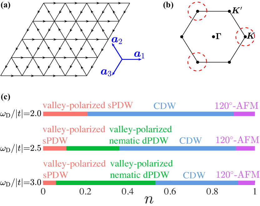
Figure 1: (a) 2D triangular lattice where the arrows indicate the direction of the orbital currents in the valley-polarized ground states. (b) The first Brillouin zone is contained within the solid lines with $\boldsymbol{\Gamma}$, $\boldsymbol{K}$, $\boldsymbol{K}^{\prime}$ points marked. The red circles indicate the occupied valleys in the valley polarized state. (c) Phase diagrams of the effective $t$-$J$-$V$ model in the limit of large system size with various electron densities, $n=N_{e}/N$. Here $\omega_{\text{D}}$ is phonon frequency in the Holstein-Hubbard model. The specific parameters used in the calculation are listed in Table 1. The PDW ordering vector is $\boldsymbol{Q}=2\boldsymbol{K}$. Abbreviations: sPDW = s-wave pair density wave; nematic dPDW = d-wave PDW plus broken lattice rotational symmetry.

Recently, three of us [60] established analytically that PDW order occurs in the 2D triangular lattice Holstein-Hubbard model in the strong-coupling limit for a narrow range of parameters. More generally, we showed that in the strong coupling limit, the low-energy physics is accurately represented by an effective model operating in a reduced subspace (with no double occupancy), that is similar to the $t$-$J$-$V$ model familiar as the strong-coupling limit of the plain Hubbard model. However, one new feature is that electron hoppings are suppressed by a Frank-Condon factor such that the effective model can be in an unfamiliar range of parameters (e.g. $t\ll J,V$). In particular, the PDW was shown to emerge for dilute electrons, negative $t$ [60], and an appropriate range of phonon frequencies. A DMRG study of the effective $t$-$J$-$V$ model on ladders with up to eight legs showed further evidence of a PDW with valley-polarization for a larger range of parameters than could be treated analytically [61]. However, further work is needed, even for the $t$-$J$-$V$ model, to establish the existence of a PDW groundstate in 2D and to extend the results beyond the dilute limit and beyond the narrowly constrained (and rather artificial) range of parameters that could be treated analytically.

We thus investigate an effective $t$-$J$-$V$ model on the 2D triangular lattice with up to 324 sites using a variational Monte Carlo (VMC) approach. Specifically, we consider a set of variational states with different patterns of broken symmetries with variable strengths of uniform (BCS) superconducting, PDW, charge-density-wave, nematic, and time-reversal symmetry breaking order parameters. We use VMC to identify the lowest variational energy among all these states. Despite known shortcomings of variational approaches to many-body systems [62], such approaches often have proven successful in identifying qualitative aspects of many ground-state phase diagrams. Parameters for the effective $t$-$J$-$V$ model [Eq. (Pair density waves in the strong-coupling two-dimensional Holstein-Hubbard model: a variational Monte Carlo study) below] we have studied are derived from the original Holstein-Hubbard model (see Table 1 above).

Our VMC study produces the quantum phase diagram shown in Fig. 1(c). Salient features are: (i) A s-wave PDW in the low electron density regions for $\omega_{\text{D}}/|t|=2$. Here, electrons are valley-polarized with spontaneous breaking of time-reversal and inversion symmetries, and the PDW arises from intra-pocket pairing with center-of-mass momentum $\boldsymbol{Q}=2\boldsymbol{K}$. (ii) For $\omega_{\text{D}}/|t|\gtrsim 2.5$, a distinct nematic d-wave PDW phase with broken lattice rotational symmetry arises at intermediate electron density. Both PDWs found in our study are commensurate which differs from the weakly incommensurate PDW found in the DMRG study [61]; as discussed below, this disagreement may be real, but may be a finite size artifact of the present calculation. (iii) PDW order disappears when the electron density is increased beyond a critical value, beyond which charge density wave (CDW) and $120^{\circ}$ antiferromagnetic ($120^{\circ}$-AFM) order appear for all $\omega_{\text{D}}$ we studied.

Model and method: In the present paper, we study the effective $t$-$J$-$V$ model on the triangular lattice:

$$H_{\text{eff}}= -t_{1}\sum_{\langle i,j\rangle,\sigma}\Big{[}c_{i\sigma}^{\dagger}c_{j\sigma}+{\rm H.c.}\Big{]}$$

$$-t_{2}\sum_{\langle i,m,j\rangle,\sigma}\Big{[}c_{i\sigma}^{\dagger}(1-2n_{m})c_{j\sigma}+{\rm H.c.}\Big{]}$$

$$-(\tau+2t_{2})\sum_{\langle i,m,j\rangle}\Big{[}s^{\dagger}_{im}s_{mj}+{\rm H.c.}\Big{]}$$

$$+J\sum_{\langle i,j\rangle}\left[\mathbf{S}_{i}\cdot\mathbf{S}_{j}-\frac{n_{i}n_{j}}{4}\right]+V\sum_{\langle i,j\rangle}n_{i}n_{j},$$ (1)

where projection onto states with no doubly occupied sites is implicit, $\langle i,j\rangle$ and $\langle i,m,j\rangle$ represent the sums over the nearest-neighbor sites and triplets of sites such that $m$ is a nearest-neighbor of two distinct sites $i$ and $j$, respectively. $c_{i\sigma}^{\dagger}$ is a creation operator of spin $\sigma$ ($\uparrow$ or $\downarrow$) at site $i$, $\mathbf{S}_{i}=c_{i\alpha}^{\dagger}\frac{\boldsymbol{\sigma}_{\alpha\beta}}{2}c_{i\beta}$ is the spin operator on site $i$, $n_{i}=\sum_{\sigma}c^{\dagger}_{i\sigma}c_{i\sigma}$ is the electron number operator, and $s_{ij}=\frac{1}{\sqrt{2}}(c_{i\uparrow}c_{j\downarrow}+c_{j\uparrow}c_{i\downarrow})=s_{ji}$ is the annihilation operator of a singlet Cooper pair on bond $\langle i,j\rangle$.

The original Holstein-Hubbard model contains four independent parameters with units of energy, the bare nearest-neighbor hopping, $t$, the bare phonon frequency, $\omega_{\text{D}}$, the phonon induced attraction, $U_{\text{e-ph}}$, and the bare Hubbard $U_{\text{e-e}}$; the parameters that appear in the effective $t$-$J$-$V$ model are functions of these [60]. The values of these - and the bare parameters they come from - are then listed in Table 1. In particular, we assume $U_{\text{e-e}}>U_{\text{e-ph}}\gg|t|$ which is what gives rise to the no double-occupancy condition. As can be seen from the table, for small $\omega_{\text{D}}$, the effective electron hoppings (e.g. $t_{1}$, $t_{2}$, and $\tau$) are strongly suppressed while the exchange interaction $J$ and density-density interaction $V$ are not significantly affected. We have not considered very low phonon frequencies here because the effective electron hoppings will become exponentially smaller, so any PDW or SC states would be expected to have such low coherence scales that they are likely preempted by other types of order.

Table 1: Parameters in the effective $t$-$J$-$V$ model [Eq. (Pair density waves in the strong-coupling two-dimensional Holstein-Hubbard model: a variational Monte Carlo study)] derived from the original Holstein-Hubbard model by fixing $t<0$, $U_{\text{e-e}}/|t|=22$, and $U_{\text{e-ph}}/|t|=18$ but varying the phonon frequency $\omega_{\text{D}}$ (see Ref. [60] for details).

$\omega_{\text{D}}/|t|$	$J/|t|$	$V/J$	$t_{1}/J$	$t_{2}/J$	$\tau/J$
2.0	0.20	0.65	$-0.056$	0.0081	0.0096
2.5	0.20	0.66	$-0.14$	0.019	0.024
3.0	0.21	0.67	$-0.24$	0.033	0.044

The VMC approach we adopt uses Gutzwiller projected trial wave functions, which is a powerful method to deal with strongly correlated systems [63, 64]. Specifically, we use Gutzwiller-projected mean-field-type wave functions of the form $P_{\rm{N_{e}}}P_{\rm G}|\Psi_{\rm mf}\rangle$ where $P_{\rm G}$ projects out any states with doubly occupied sites, $P_{\rm{N_{e}}}$ is the projection operator onto states with a fixed number of electrons $N_{e}$, and $|\Psi_{\rm mf}\rangle$ is constructed as the ground state of the following quadratic (mean-field-like) Hamiltonian [65],

$$H_{\text{mf}} =\sum_{i,l}\Big{(}T_{i,a_{l}}\mathcal{F}_{i}^{\dagger}\mathcal{F}_{i+a_{l}}+\Delta_{i,a_{l}}\mathcal{F}_{i}^{\dagger}\bar{\mathcal{F}}_{i+a_{l}}+{\rm H.c.}\Big{)}$$

$$~{}~{}~{}+\sum_{i}\Big{(}\Lambda_{i}\mathcal{F}_{i}^{\dagger}\mathcal{F}_{i}+\mathbf{M}_{i}\cdot\mathcal{F}_{i}^{\dagger}\frac{\boldsymbol{\sigma}}{2}\mathcal{F}_{i}\Big{)},$$ (2)

where $\mathcal{F}_{i}=(c_{i\uparrow},c_{i\downarrow})^{\mathsf{T}}$, $\bar{\mathcal{F}}_{i}=(c_{i\downarrow}^{\dagger},-c_{i\uparrow}^{\dagger})^{\mathsf{T}}$, and $\boldsymbol{a}_{l}$ with $l\in\{1,2,3\}$ are primitive vectors shown in Fig. 1(a). Here $T_{i,a_{l}}$ are effective complex hopping amplitudes, $\Delta_{i,a_{l}}$ effective pair-fields, $\Lambda_{i}$ is a site energy, and $\mathbf{M}_{i}$ is an effective Zeeman field that induces various patterns of magnetic order. A pattern of phase order for the hopping amplitudes is assumed, as shown in Fig. 1(a), where the arrows indicate the direction of positive $\phi_{i,a_{l}}$ in $T_{i,a_{l}}=|T_{i,a_{l}}|e^{i\phi_{i,a_{l}}}$ with $\phi_{i,a_{l}}\in(-\pi,\pi$].

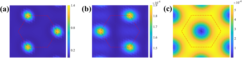
Figure 2: Properties of the lowest-energy variational sPDW state for the model with $\omega_{\text{D}}/|t|=2$ and filling $n=1/12$. (a) The occupation number in momentum space $n(\boldsymbol{k})=\sum_{\sigma}\langle c^{\dagger}_{\boldsymbol{k}\sigma}c_{\boldsymbol{k}\sigma}\rangle$ as a function of $\boldsymbol{k}$ in the first Brillouin zone (represented by the red dashed line) is plotted in color scale; it is clear that the electrons are valley polarized. (b) The static SC structure factor $|S^{\text{SC}}_{\boldsymbol{a}_{1},\boldsymbol{a}_{1}}(\boldsymbol{k})|$ plotted in color scale; (c) The static spin structure factor $S(\boldsymbol{k})$ plotted in color scale.

The various mean-field wave functions that we have analyzed correspond to different patterns and magnitudes of the variational parameters in Eq. (Pair density waves in the strong-coupling two-dimensional Holstein-Hubbard model: a variational Monte Carlo study). A PDW state corresponds to a spatial varying pairing field,

$$\Delta_{i,a_{l}}=\left\{\begin{array}[]{ll}\tilde{\Delta}_{l}(e^{i\boldsymbol{q}\cdot\boldsymbol{r}_{i}}+e^{-i\boldsymbol{q}\cdot\boldsymbol{r}_{i}}),&\text{LO-type}\vspace{2mm}\\ \tilde{\Delta}_{l}e^{i\boldsymbol{q}\cdot\boldsymbol{r}_{i}},&\text{FF-type}\end{array}\right.$$ (5)

where $\tilde{\Delta}_{l}$ represents pairing field on bonds along $\boldsymbol{a}_{l}$ direction. Whenever $\boldsymbol{q}=\boldsymbol{K}$, which is the high-symmetry momentum point respecting $C_{3}$ rotational symmetry, we can set $\tilde{\Delta}_{l}=\Delta_{s}$, $\Delta_{d}\cos(2\theta_{l})$, or $\Delta_{d+id}e^{2i\theta_{l}}$ corresponding to s-wave PDW, or d-wave nematic PDW, d+id-wave PDW, respectively ($\theta_{l}$ being the azimuth angle of $\boldsymbol{a}_{l}$). The s-wave PDW is invariant under $C_{3}$, while a d-wave PDW, in which $\theta_{l}$ can be $0$, $2\pi/3$, or $4\pi/3$, is necessarily nematic [66, 67, 68]. Note that $\boldsymbol{q}$ is the center of mass momentum of the pairing in the mean-field wave function before Gutzwiller projection and it is a variational parameter. A translationally-invariant SC trial wave function corresponds to $\boldsymbol{q}=0$. We also consider CDW order through modulated $\Lambda_{i}$, $120^{\circ}$-AFM order through three-sublattice local field $\mathbf{M}_{i}$, as well as states with co-existing multiple broken symmetries [for details see Supplemental Material (SM)].

In implementing the VMC calculations, the projections $P_{\rm{N_{e}}}$ and $P_{\rm G}$ must be enforced exactly. The central quantity to be computed is the variational energy, $E(x)=\langle\Psi(x)|H_{\text{eff}}|\Psi(x)\rangle/\langle\Psi(x)|\Psi(x)\rangle$, where $|\Psi(x)\rangle=P_{\rm{N_{e}}}P_{\rm G}|\Psi_{\rm mf}(x)\rangle$, and $x$ denotes the variational parameters ($T_{i,a_{l}}$, $\Delta_{i,a_{l}}$, $\Lambda_{i}$, $\mathbf{M}_{i}$, $\boldsymbol{q}$). The calculations have been performed on 2D triangular lattices with up to $18\times 18$ sites and periodic boundary conditions along both directions (namely on a torus).

VMC results: Here we study physics of the effective $t$-$J$-$V$ model whose parameters are listed in Table 1. The main results are the VMC phase diagrams as a function of electron densities shown in Fig. 1(c). For relatively small electron density, the ground state is a valley-polarized s-wave PDW state, and the region of sPDW decreases with increasing the phonon frequency. For a range of relatively large phonon frequencies, a d-wave PDW state arises at somewhat larger electron densities. The dPDW state is nematic in the sense that it breaks lattice rotational symmetry spontaneously. Both sPDW and dPDW ground states exhibit spontaneous valley polarization and hence break time-reversal and inversion symmetries. If the density of electrons is further increased, CDW and $120^{\circ}$-AFM states appear. Below we shall discuss in detail the properties of the PDW states.

Table 2: Mean-field Ansätze for different projected wave functions appearing in the phase diagrams, where $\theta_{l}$ is the azimuth angle of $\boldsymbol{a}_{l}$.

	$T_{i,a_{l}}$	$\Delta_{i,a_{l}}$	$\Lambda_{i}$	$\mathbf{M}_{i}$
sPDW	$T$	$\Delta_{s}e^{i\boldsymbol{q}\cdot\boldsymbol{r}_{i}}$	$\Lambda_{0}$	0
dPDW	$T$	$\Delta_{d}\cos(2\theta_{l})e^{i\boldsymbol{q}\cdot\boldsymbol{r}_{i}}$	$\Lambda_{0}$	0
CDW	$T$	0	$\Lambda_{0}+\Lambda_{1}\cos(\boldsymbol{q}\cdot\boldsymbol{r}_{i})$	0
$120^{\circ}$	$T$	0	$\Lambda_{0}$	$120^{\circ}$-AFM

We find that for low electron density the Gutzwiller projected ground state with the lowest variational energy is always valley polarized. Valley polarization breaks inversion and time-reversal symmetries, but is consistent with translation symmetry. It also features an orbital loop current order of the sort shown in Fig. 1(a) - which is a form of intra-unit cell orbital antiferromagnetism (or altermagnetism to use a new buzz word). Indeed, typically we find fully valley polarized states, so as shown in Fig. 1(b) the Fermi surface encloses only one of two related high symmetry points, taken to be $\boldsymbol{K}$ in the figure. In the presence of such order, if SC is to arise at all it is natural to expect PDW ordering since pairing two electrons in the same valley results in Cooper pairs with center-of-mass momentum $\approx 2\boldsymbol{K}$. Indeed, as discussed below, although we treat the ordering vector $\boldsymbol{q}$ as a variational parameter as shown in Table 2, so long as $\boldsymbol{q}\approx\boldsymbol{Q}\equiv 2\boldsymbol{K}$, after Gutzwiller projection we obtain a PDW state with ordering vector exactly equal to $\boldsymbol{Q}$.

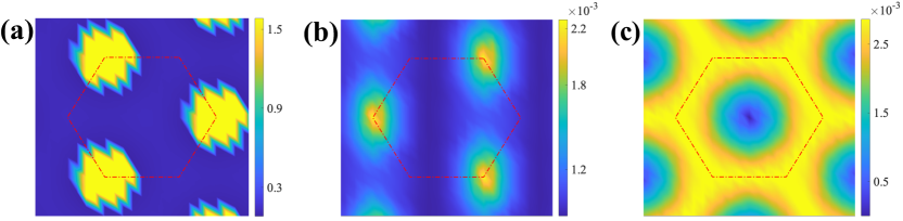
Figure 3: Properties of the dPDW state with $\omega_{\text{D}}/|t|=3$, $n=5/12$. (a) The occupation number in momentum space $n(\boldsymbol{k})$; (b) The static SC structure factor $|S^{\text{SC}}_{\boldsymbol{a}_{1},\boldsymbol{a}_{1}}(\boldsymbol{k})|$; (c) The static spin structure factor $S(\boldsymbol{k})$. The red dotted box represents the first Brillouin zone.

To see if the projected state exhibits valley polarization in the low electron density region, we calculate the electron occupation number in momentum space,

$$n(\boldsymbol{k})=\frac{1}{N}\sum_{i,j,\sigma}e^{i\boldsymbol{k}\cdot(\boldsymbol{r}_{i}-\boldsymbol{r}_{j})}\langle c_{i\sigma}^{\dagger}c_{j\sigma}\rangle=\sum_{\sigma}\langle c^{\dagger}_{\boldsymbol{k}\sigma}c_{\boldsymbol{k}\sigma}\rangle$$ (6)

where $N$ is the number of sites of the lattice under study. As shown in Fig. 2(a), essentially all of the electron occupation is concentrated at momenta around the $\boldsymbol{K}$ valley, and the maximum value of $n(\boldsymbol{k})$ is always larger than $1$. This feature is inherited directly from the pre-projected valley-polarized wave function ansatz. Naturally, as the electron density increases, the effective Fermi surface of sPDW increases proportionately. (See the SM.)

To characterize the SC state, we calculate the static superconducting structure factor in the projected state,

$$S^{\rm{SC}}_{\boldsymbol{a},\boldsymbol{a}^{\prime}}(\boldsymbol{k})=\frac{1}{N^{2}}\sum_{\boldsymbol{r}_{i},\boldsymbol{r}_{j}}\mathrm{e}^{\mathrm{i}\boldsymbol{k}\cdot(\boldsymbol{r}_{i}-\boldsymbol{r}_{j}})\langle\Delta^{\dagger}_{\boldsymbol{a}}(\boldsymbol{r}_{i})\Delta_{\boldsymbol{a}^{\prime}}(\boldsymbol{r}_{j})\rangle,$$ (7)

where $\Delta_{\boldsymbol{a}}^{\dagger}(\boldsymbol{r}_{i})=(c_{\boldsymbol{r}_{i},\uparrow}^{\dagger}c_{\boldsymbol{r}_{i}+\boldsymbol{a},\downarrow}^{\dagger}+c_{\boldsymbol{r}_{i}+\boldsymbol{a},\uparrow}^{\dagger}c_{\boldsymbol{r}_{i},\downarrow}^{\dagger})$ creates a singlet pair on the nearest-neighboring bonds along the $\boldsymbol{a}$ direction. We find that the SC structure factor peaks at momentum $\boldsymbol{Q}=2\boldsymbol{K}\equiv\boldsymbol{K}^{\prime}$, as shown in Fig. 2(b), over the entire range of density we have explored and for any reasonable choice of $\boldsymbol{q}$ in the trial wave function before projection. We take this as indicating the existence of PDW order that arises from intra-pocket pairing with a commensurate center of mass momentum, as shown in Fig. 1(b). As the electron density increases, the peak of the SC structure factor becomes higher (see the SM for details). Note that DMRG calculations of the model on cylinders with $L_{x}\gg L_{y}$ find an incommensurate s-wave PDW [61], which we attribute to the largeness of $L_{x}$ of the length of long cylinders studied by DMRG (see the SM for more details); namely we conjecture that the PDW obtained from VMC might be weakly incommensurate, consistent with the DMRG result, if the VMC study was extended to sufficiently large lattices.

To determine magnetic properties of the projected states, we compute the static spin structure factor $S(\boldsymbol{k})=\frac{1}{N^{2}}\sum_{ij}e^{i\boldsymbol{k}\cdot(\boldsymbol{r}_{i}-\boldsymbol{r}_{j})}\langle\boldsymbol{S}_{\boldsymbol{r}_{i}}\cdot\boldsymbol{S}_{\boldsymbol{r}_{j}}\rangle$. As shown in Fig. 2(c), for the sPDW state there appear no prominent peaks in the $S(\boldsymbol{k})$. This is consistent with the observation that in this range of parameters, the variation energy is minimized when $\mathbf{M}_{i}=\mathbf{0}$. There is no long-range magnetic ordering in the sPDW state although the valley-polarization spontaneously breaks time-reversal symmetry.

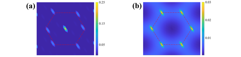
Figure 4: (a) The density structure factor $C(\boldsymbol{k})$ of the CDW order with $\omega_{\text{D}}/|t|=2.5$, $n=0.5$; (b) The static spin structure factor $S(\boldsymbol{k})$ of the $120^{\circ}$-AFM order with $\omega_{\text{D}}/|t|=2.5$, $n=0.94$. The red dotted box represents the first Brillouin zone.

As the PDW ordering vector is at high symmetry momentum point $\boldsymbol{K}$, the internal structure of the PDW can be s-wave, d-wave, and even d+id. For $\omega_{\text{D}}/|t|=2$, we find that the energy of the optimized sPDW state is always lower than that of the dPDW state from low to intermediate electron density. However, for $\omega_{\text{D}}/|t|=2.5$ and $\omega_{\text{D}}/|t|=3$, we find that the dPDW state is lower for the large density end of the range we have explored, as shown in Fig. 1(c). In common with what we found in the sPDW case, the variationally determined hopping parameters $T_{i,a_{l}}$ are such that time-reversal and inversion symmetries are spontaneously broken, and the electrons are valley polarized, as shown in Fig. 3(a), and the superconducting state has pairing momentum $\boldsymbol{Q}=2\boldsymbol{K}\equiv\boldsymbol{K}^{\prime}$, as shown in Fig. 3(b). The spin structure factor of the dPDW state is shown in Fig. 3(c). We find that the region of dPDW increases with increasing phonon frequency, as shown in Fig. 1(c). The dPDW state spontaneously breaks a discrete $C_{3}$ rotation symmetry of the triangular lattice, namely, it has nematic order. It is interesting to note that for the $t$-$J$-$V$ model studied here the nematic dPDW state has lower energy than the PDW with d+id pairing, which is also allowed by symmetry [68, 67].

It is important to stress that the sign of the bare hopping $t$ in the Holstein-Hubbard model is quite crucial to induce PDW ground states, as anticipated in Ref. [60]. When $t>0$ (resulting in only a change in the sign of $t_{1}$ in the effective $t$-$J$-$V$ model), the ground state found in our VMC simulations at low electron density is a uniform d-wave SC rather than a PDW.

For completeness, we have cursorily explored the evolution of the ground-state to larger values of the electron density $n$, beyond the PDW ordering range. Here, the typical ground state is a CDW without magnetic orders. The CDW is obtained from the projection of a mean-field state with spatial variations of on-site energy $\Lambda_{i}$, as shown in Table 2. We calculated CDW states with different momenta to obtain the state with the lowest possible energy. We find that the momentum $\boldsymbol{k}^{*}$ of the optimized CDW state is typically incommensurate, with an amplitude that decreases when increasing $n$. The density structure factor $C(\boldsymbol{k})=\frac{1}{N^{2}}\sum_{\boldsymbol{r}_{i},\boldsymbol{r}_{j}}e^{i\boldsymbol{k}\cdot(\boldsymbol{r}_{i}-\boldsymbol{r}_{j})}\langle n_{\boldsymbol{r}_{i}}n_{\boldsymbol{r}_{j}}\rangle$ is indeed peaked at the incommensurate $\pm\boldsymbol{k}^{*}$ as well as at the $\boldsymbol{\Gamma}$ point (which represents the uniform component of the charge density), as shown in Fig. 4(a). In other words, it is an incommensurate CDW.

At half filling ($n=1$), the effective model is equivalent to the spin-1/2 antiferromagnetic Heisenberg model on the triangular lattice whose ground state is believed to be the three-sublattice $120^{\circ}$ magnetically ordered state [69, 70, 71, 72, 73]. Our VMC results for half-filling also show that the $120^{\circ}$-AFM order is the state with the lowest energy. For example, strong peaks at $\boldsymbol{K}$ and $\boldsymbol{K}^{\prime}$ points emerge in the static spin structure factor $S(\boldsymbol{k})$ [Fig. 4(b)]. Furthermore, the $120^{\circ}$-AFM ordered state is stable when electron density is slightly away from half-filling although the single-particle excitation spectrum is gapless.

Discussions and conclusions: The effects of relatively weak electron-phonon coupling are well understood - typically they lead to uniform SC or, in special circumstances, CDW order. Strong electron-phonon coupling, by contrast, quenches electron mobility through polaron formation, when (as is typically the case) $\omega_{\text{D}}$ is small compared to the electronic bandwidth. This generally leads to insulating CDW order - possibly (in the presence of strong electron-electron repulsion) with coexisting magnetism. The present study deals with a relatively unexplored range of parameters, where the electron-phonon coupling is reasonably strong, but the phonon frequencies and electronic energies are comparable. While such a regime of parameters is unlikely to arise in most simple metals, it may be relevant in various artificial “narrow-band” systems that have been the focus of considerable recent experimental interest, or (more speculatively) in strongly correlated systems where the electron effective mass can be highly renormalized.

For PDW states of LO-type, secondary orders such as CDW and uniform charge-4e pairing can generically emerge, as can be understood from the perspective of Ginzburg-Landau (GL) theory [8, 74, 75]. Our VMC calculations suggest that the ground state at low electron densities in an appropriate range of phonon frequencies is a PDW state of FF-type, namely a valley-polarized PDW state (s-wave or d-wave) whose Cooper pairs condense at a single momentum $\boldsymbol{Q}=2\boldsymbol{K}$. Consequently, there is no induced CDW or uniform charge-4e SC order. However, there are higher harmonic orders consisting of charge-4e PDW order with $2\boldsymbol{Q}$ and charge-6e uniform SC order with $3\boldsymbol{Q}\equiv\boldsymbol{0}$ since $3\boldsymbol{K}$ is a reciprocal lattice vector.

In summary, our VMC calculations imply that (s-wave or d-wave) PDW ground state phases occur in the Holstein-Hubbard model on the triangular lattice for moderately strong doping, relatively high phonon frequencies, in a range of (low) electron densities that depends on the phonon frequency, as shown in Fig. 1(c). The obtained PDW state is valley-polarized with staggered loop currents, spontaneously breaking both time-reversal and inversion symmetries, which can be employed to realize superconducting diode effect [76, 77, 78, 79]. One interesting open question concerns the nature of the quantum phase transition between sPDW and dPDW. Moreover, how these different PDWs respond to external magnetic fields is another interesting issue for investigation [80]. We believe that our work provides strong support for possible realization of various PDW states in 2D quantum systems with both strong electron-electron and electron-phonon interactions.

Acknowledgement: This work was supported in part by the NSFC under Grant No. 12347107 and the Postdoctoral Science Foundation of China under Grant No. 2021M690093. ZH and SAK were funded in part by the Department of Energy, Office of Basic Energy Sciences, under Contract No. DE-AC02-76SF00515 at Stanford. HY was supported in part by the New Cornerstone Science Foundation through the Xplorer Prize.

I Supplemental Material

I.1 A. Different Ansätze and competing states

In the following, we will show more Gutzwiller-projected mean-field states with different pairing patterns in the VMC framework. As shown in the main text, the general mean-field-like Hamiltonian (with spin-singlet pairing terms) can be written as,

$$H_{\text{mf}}= \sum_{i,l}\Big{(}T_{i,a_{l}}\mathcal{F}_{i}^{\dagger}\mathcal{F}_{i+a_{l}}+\Delta_{i,a_{l}}\mathcal{F}_{i}^{\dagger}\bar{\mathcal{F}}_{i+a_{l}}+{\rm H.c.}\Big{)}+\sum_{i}\Big{(}\Lambda_{i}\mathcal{F}_{i}^{\dagger}\mathcal{F}_{i}+\mathbf{M}_{i}\cdot\mathcal{F}_{i}^{\dagger}\frac{\boldsymbol{\sigma}}{2}\mathcal{F}_{i}\Big{)},$$ (S1)

$${\rm where}\qquad\Delta_{i,a_{l}}=\left\{\begin{array}[]{ll}\tilde{\Delta}_{l}(e^{i\boldsymbol{q}\cdot\boldsymbol{r}_{i}}+e^{-i\boldsymbol{q}\cdot\boldsymbol{r}_{i}}),&\text{LO-type}\vspace{2mm}\\ \tilde{\Delta}_{l}e^{i\boldsymbol{q}\cdot\boldsymbol{r}_{i}},&\text{FF-type}\end{array}\right.$$ (S4)

where $|\Psi_{\rm mf}(x)\rangle$ is the mean-field ground state, and $x$ denotes the variational parameters ($T_{i,a_{l}}$, $\Delta_{i,a_{l}}$, $\Lambda_{i}$, $\mathbf{M}_{i}$, $\boldsymbol{q}$). Using the above trial wave functions and the Gutzwiller projection enforcing the no-double-occupancy constraint (i.e. $P_{\rm G}=\prod_{i}(1-n_{i,\uparrow}n_{i,\downarrow})$), we could calculate the expectation values of the original effective $t$-$J$-$V$ model employing the standard VMC approach. Specifically, the projected trial wave function becomes $|\Psi(x)\rangle=P_{\rm{N_{e}}}P_{\rm G}|\Psi_{\rm mf}(x)\rangle$ with fixed number of electrons $N_{e}$ through $P_{\rm{N_{e}}}$.

The PDW state is constructed by spatial variations of the paring parameter, $\Delta_{i,a_{l}}$ with $l\in\{1,2,3\}$. Note that $\boldsymbol{q}$ is the center-of-mass momentum of the pairing in the mean-field wave function. Indeed, from a symmetry point of view, (i) if the PDW ordering vector is at the high symmetry point (i.e. $\boldsymbol{\Gamma}$, $\boldsymbol{K}$, or $\boldsymbol{K}^{\prime}$), the classification of s- and d-wave is meaningful, and then the s-wave PDW is invariant under $C_{6}$ rotation while the d-wave PDW is necessarily nematic due to local structure; (ii) the rotation symmetry is necessarily broken even in an s-wave pairing if the PDW ordering vector $\boldsymbol{q}$ is generic not at high symmetry point. Thus, there is no constraint on $\Delta_{i,a_{l}}$ for the generic momentum $\boldsymbol{q}$, which means there is no relation between the strength of pairing among three distinct bond directions, namely a generic PDW. In other words, for the generic $\boldsymbol{q}$, the sPDW and dPDW are just two special choices of former factors. For $\boldsymbol{q}=\boldsymbol{K}$ or $\boldsymbol{K}^{\prime}$, it has $C_{3}$ rotation symmetry such that one can sharply define sPDW and dPDW. We have also constructed uniform SC states (with setting $\boldsymbol{q}=0$), CDW (through modulated $\Lambda_{i}$), $120^{\circ}$-AFM order (via three-sublattice local field $\mathbf{M}_{i}$), and other mixed states with coexisting multiple broken symmetries (such as uniform SC+PDW states, uniform SC+CDW states, PDW+CDW states, uniform SC+$120^{\circ}$-AFM states, CDW+$120^{\circ}$-AFM states, and the like). Additionally, we have constructed spin-triplet SC trial wave functions, but their energies are much higher than spin-singlet SC states after Gutzwiller projection, and thus we don’t consider them here.

Table S1: The optimized energy of several candidate states of the effective $t$-$J$-$V$ model obtained on a system of size $12\times 12$ with various electric densities. Here we don’t show $120^{\circ}$-AFM order (due to almost zero $\mathbf{M}_{i}$ after Gutzwiller projection) and possible mixed states (because of higher variational energies). Note that the optimized energy means the total energy of the original model instead of the energy per site and we set $|t|=1$ as an energy unit.

	$\omega_{\text{D}}/|t|=2.0$			$\omega_{\text{D}}/|t|=2.5$			$\omega_{\text{D}}/|t|=3.0$
	$n=1/6$	$n=1/4$	$n=1/3$	$n=1/12$	$n=1/6$	$n=5/12$	$n=1/4$	$n=1/3$	$n=5/12$
Uniform s-wave SC	$-0.7287$	$-0.7599$	$-0.2898$	$-1.0018$	$-1.6425$	$-0.5895$	$-3.4833$	$-3.4173$	$-2.3484$
Valley-polarized sPDW	$-0.7878$	$-0.7837$	$-0.3048$	$-1.0116$	$-1.6408$	$-0.5904$	$-3.4818$	$-3.4182$	$-2.3573$
Valley-unpolarized sPDW	$-0.7738$	$-0.7788$	$-0.2706$	$-1.0103$	$-1.6322$	$-0.5613$	$-3.4816$	$-3.3980$	$-2.3557$
Uniform d-wave SC	$-0.7292$	$-0.7588$	$-0.3062$	$-1.0009$	$-1.6436$	$-0.5941$	$-3.4845$	$-3.4103$	$-2.3633$
Valley-polarized dPDW	$-0.7292$	$-0.7603$	$-0.3085$	$-1.0008$	$-1.6441$	$-0.5881$	$-3.4867$	$-3.4209$	$-2.3675$
Valley-unpolarized dPDW	$-0.7146$	$-0.7394$	$-0.2882$	$-0.9476$	$-1.5717$	$-0.4153$	$-3.4537$	$-2.9171$	$-2.1150$
Uniform d+id-wave SC	$-0.7275$	$-0.7561$	$-0.3057$	$-1.0012$	$-1.6424$	$-0.5875$	$-3.4851$	$-3.4114$	$-2.3579$
Valley-polarized d+idPDW	$-0.7255$	$-0.7577$	$-0.3038$	$-1.0007$	$-1.6415$	$-0.5789$	$-3.4811$	$-3.4102$	$-2.3539$
Valley-unpolarized d+idPDW	$-0.7098$	$-0.7042$	$-0.3037$	$-0.9816$	$-1.5998$	$-0.3983$	$-3.4583$	$-2.8440$	$-2.2573$
CDW	$-0.6596$	$-0.8876$	$-0.5466$	$-0.9175$	$-1.4568$	$-0.7589$	$-2.8914$	$-3.1204$	$-1.8722$

Based on the standard VMC method, a direct comparison of the optimized energies of several candidate states of some typical parameter sets is shown in Table S1. From the table, our VMC calculations show that there is a phase transition (from valley-polarized sPDW to CDW) between electron densities $n=1/6$ and $n=0.25$ for $\omega_{\text{D}}/|t|=2$. Thus, the favored ground state is the s-wave PDW when the electron density is sufficiently low, consistent with the results of the previous perturbation approach [60]. And for $\omega_{\text{D}}/|t|=2.5$, the energy of the valley-polarized sPDW state is slightly lower than that of the d-wave PDW for $n=1/6$. Therefore, there is a direct phase transition from sPDW to dPDW below electron density $n=1/6$. As the phonon frequency increases, there is a much larger region for the dPDW phase for $\omega_{\text{D}}/|t|=3$. Here, we also compare the energies of valley-polarized PDW states with different momentums $\boldsymbol{q}s$ and find that their energies are no better (not shown here). From our VMC simulations, the optimized hopping parameters $T_{i,a_{l}}$ are complex numbers (which usually break time-reversal and inversion symmetries), and the symmetry between momenta $\boldsymbol{k}$ and $-\boldsymbol{k}$ points in the dispersion is indeed broken. If electron density is small, the electrons will first occupy the momentum points where the energies are lower (i.e. valley polarization near the $\boldsymbol{K}$ point in Fig. 1(b)), and Gutzwiller projection can spontaneously select out the pairing momentum $\boldsymbol{Q}=2\boldsymbol{K}\equiv\boldsymbol{K}^{\prime}$. Thus the mechanism of PDWs in the present model is firstly valley polarization with staggered loop currents and then intra-pocket pairing.

Actually, in the VMC framework, we have considered generic PDW states (namely $\tilde{\Delta}_{l}$ are considered as three independent variational parameters), and find that their energies are no better than those of the corresponding s-wave or d-wave PDW in the larger lattice size. Additionally, the effect of small $t_{2}$ and $\tau$ terms in the effective $t$-$J$-$V$ model on the 2D triangular lattice is almost negligible, at most slightly changing the phase boundary. To summarize, the hopping $t_{1}$, the exchange interaction $J$, and the density-density interaction $V$ determine the key physics of the system under study.

Taken together, our VMC simulations clearly show that the valley-polarized (either s-wave or d-wave) PDW state can be favored as the ground state of the effective $t$-$J$-$V$ model [for details see Fig. 1(c)]. It is possible that the sPDW state disappears with further increase of the phonon frequency. However, further studies are needed to determine the upper critical phonon frequency at which the valley-polarized sPDW disappears.

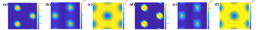
Figure S1: Properties of PDW states with various phonon frequencies and electron densities. (a) and (d): The occupation number in momentum space $n(\boldsymbol{k})$; (b) and (e): The static SC structure factor $|S^{\text{SC}}_{\boldsymbol{a}_{1},\boldsymbol{a}_{1}}(\boldsymbol{k})|$; (c) and (f): The static spin structure factor $S(\boldsymbol{k})$. The left three figures [(a)$\sim$(c)] are for sPDW with setting $\omega_{\text{D}}/|t|=2$ and $n=1/6$, and right three figures [(d)$\sim$(f)] are for dPDW with setting $\omega_{\text{D}}/|t|=3$ and $n=1/4$. The red dotted box represents the first Brillouin zone.

I.2 B. Properties of PDWs with various electron densities

As shown in Figs. 2, 3, and S1, the properties of PDW states are stable for electron densities regardless of whether the ground state is a valley-polarized sPDW or dPDW state. Specifically, for both PDW states, the static spin structure factor has not changed qualitatively while the effective Fermi surface (as shown in the occupation number in momentum space $n(\boldsymbol{k})$) becomes larger and larger as we increase electron densities in the PDW phase. Moreover, the peak of the static SC structure factor in the PDW phase becomes higher as the electron density increases. Thus, the properties of the sPDW (or dPDW) are consistent in the corresponding region of the phase diagrams. In particular, the valley polarization (indicating an orbital loop current order) breaks time-reversal and inversion symmetries independently for the SC order. The valley-polarized sPDW doesn’t break any other symmetries, while the valley-polarized dPDW breaks the remaining $C_{3}$ rotation symmetry, namely, exhibiting a nematic order.

To estimate the possible SC transition temperature at low electron density, we have calculated the static SC structure factor $S^{\text{SC}}_{\boldsymbol{a}_{1},\boldsymbol{a}_{1}}(\boldsymbol{k})$ of sPDW (fixing $\omega_{\text{D}}/|t|=2$, $n\approx 1/12$) on different lattice sizes, and thus the height at the $\boldsymbol{K}^{\prime}$-point becomes a small finite value ($\sim 5\times 10^{-5}$) in the thermodynamic limit. If we assume that the energy scale of the bare hopping $t$ is about 100 meV, the pairing order parameter becomes $\Delta\sim J\times\sqrt{|S^{\text{SC}}_{\boldsymbol{a}_{1},\boldsymbol{a}_{1}}(\boldsymbol{K^{\prime}})|}$ $\sim 0.1$ meV, which means the SC transition temperature is about 1 $\rm K$. Roughly speaking, at this low electron density, the above pairing order parameter $\Delta$ is an order of magnitude smaller than the hopping $t_{1}$ in the effective model.

I.3 C. Charge-density-wave orders with different patterns

In the following, we consider other possible charge-density-wave patterns besides the CDW mentioned above (by modulated $\Lambda_{i}$ with momentum $\boldsymbol{q}$). For simplicity, we consider only two types of CDW orders with different patterns (which means translation symmetry-breaking patterns), as shown in Fig. S2. These CDW-type trial wave functions (without magnetic orders) can be constructed by the projected CDW-type mean-field Hamiltonian,

$$H_{\text{mf}}^{\text{CDW}} =\sum_{i,l}\Big{(}T_{i,a_{l}}\mathcal{F}_{i}^{\dagger}\mathcal{F}_{i+a_{l}}+{\rm H.c.}\Big{)}+\sum_{i}\Lambda_{i}\mathcal{F}_{i}^{\dagger}\mathcal{F}_{i},$$ (S5)

where $|\Psi_{\rm mf}^{\rm{CDW}}\rangle$ is the mean-field ground state of the CDW-type mean-field Hamiltonian above, and the pattern $\{\Lambda_{i}\}$ determines different CDW orders. Therefore, for the CDW_2×2 order [Fig. S2(a)], the trial wave function is $|\Psi^{\rm{CDW_{2\times 2}}}(x)\rangle=P_{\rm{N_{e}}}P_{\rm G}|\Psi_{\rm mf}^{\rm{CDW_{2\times 2}}}(x)\rangle$, where $x$ denotes the variational parameters ($T_{i,a_{l}}$, $\Lambda_{1}$, $\Lambda_{2}$, $\Lambda_{3}$, $\Lambda_{4}$). Similarly, for the CDW_3×3 order [Fig. S2(b)], the trial wave function is $|\Psi^{\rm{CDW_{3\times 3}}}(x)\rangle=P_{\rm{N_{e}}}P_{\rm G}|\Psi_{\rm mf}^{\rm{CDW_{3\times 3}}}(x)\rangle$, where $x$ denotes the variational parameters ($T_{i,a_{l}}$, $\Lambda_{1}$, $\Lambda_{2}$, $\Lambda_{3}$, $\Lambda_{4}$, $\Lambda_{5}$, $\Lambda_{6}$, $\Lambda_{7}$, $\Lambda_{8}$, $\Lambda_{9}$). Using the above wave functions, we calculate the expectation values of the original effective $t$-$J$-$V$ model utilizing the VMC approach. A direct comparison of the optimized energies of CDW orders with different phonon frequencies and electron densities is shown in Table S2. As a result, we find that the energy of the CDW state with $\Lambda_{i}=\Lambda_{0}+\Lambda_{1}\cos(\boldsymbol{q}\cdot\boldsymbol{r}_{i})$ is the lowest one among them, where the momentum $\boldsymbol{q}$ dependents on the specific electron density, i.e. it has an incommensurate order. We also check the energies of these CDW orders on larger system sizes and find that the results from VMC are consistent. Perhaps, some CDW patterns with rather large unit cells will be further considered in the VMC framework.

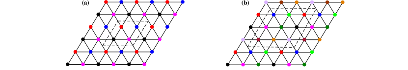
Figure S2: The patterns of two types of CDW orders. (a) CDW_2×2 order with a $2\times 2$ pattern; (b) CDW_3×3 order with a $3\times 3$ pattern. Note that different colors indicate different site-energy parameters $\Lambda_{i}$ in Eq. (S5). The black dotted box represents the unit cell of the corresponding CDW order.

Table S2: The optimized energy of CDWs obtained on a system of size $12\times 12$ with various phonon frequencies and electron densities. The patterns of CDW_2×2 and CDW_3×3 are shown in Fig. S2 above. Note that the optimized energy means the total energy of the original model instead of the energy per site and we set $|t|=1$ as an energy unit.

	$\omega_{\text{D}}/|t|=2.0$, $n=1/3$	$\omega_{\text{D}}/|t|=2.5$, $n=5/12$	$\omega_{\text{D}}/|t|=3.0$, $n=5/9$
CDW	$-0.5466$	$-0.7589$	0.3069
CDW2×2	$-0.3156$	$-0.5962$	0.6514
CDW3×3	$-0.3140$	$-0.5974$	0.6539

Table S3: The optimized energy of two candidate states of the effective $t$-$J$-$V$ model (with setting $\omega_{\text{D}}/|t|=3$) obtained on the torus of different geometric shapes (fixed the total lattice number, $N=N_{x}\times N_{y}=144$) with various electron densities. Note that the optimized energy means the total energy of the original model instead of the energy per site and we set $|t|=1$ as an energy unit.

	$12\times 12$			$24\times 6$			$48\times 3$
	$n=1/6$	$n=1/4$	$n=1/3$	$n=1/6$	$n=1/4$	$n=1/3$	$n=1/6$	$n=1/4$	$n=1/3$
Valley-polarized sPDW	$-2.9233$	$-3.4818$	$-3.4182$	$-2.8347$	$-3.3807$	$-3.3551$	$-3.5668$	$-4.3629$	$-3.9224$
Valley-polarized dPDW	$-2.9250$	$-3.4867$	$-3.4209$	$-2.8337$	$-3.3828$	$-3.4219$	$-3.5370$	$-4.2837$	$-3.9205$

I.4 D. The finite-size effect of the effective $t$-$J$-$V$ model

As noted in the main text, the phase diagram of the effective $t$-$J$-$V$ model (with setting $\omega_{\text{D}}/|t|=3$) obtained by VMC is inconsistent with the results obtained by DMRG on cylinders (i.e., highly anisotropic ladder geometries composed of a relatively small number of legs) [61]. The DMRG results show that the ground state is only a valley-polarized sPDW (resulting from intra-pocket pairing with a weakly incommensurate center of mass momentum) in a large region of low electron density, while the VMC calculations show a valley-polarized sPDW for a small region with very low electron density and a valley-polarized nematic dPDW for a large region [see Fig. 1(c)].

To understand the issue, we have studied the effective $t$-$J$-$V$ model on the quasi-one-dimensional system (which is like the lattice geometry in DMRG). As shown in Table S3, we indeed find a very broad regime of the valley-polarized sPDW phase whose size increases as $N_{y}$ decreases (when the total lattice number $N=N_{x}\times N_{y}$ is fixed). Specifically, for the $48\times 3$ case, the phase transition from sPDW to dPDW may be larger than the electron density $n=1/3$, while the phase transition from sPDW to dPDW is much less than the electron density $n=1/6$ for the $12\times 12$ case. In a sense, the more the system resembles a quasi-one-dimensional geometry, the stronger the tendency for the ground state to be sPDW. To summarize, the above VMC results are qualitatively consistent with those obtained by DMRG (except for commensurate in VMC and weakly incommensurate in DMRG). However, the lattice size we can simulate with VMC is very limited and not large enough so far. We conjecture that whether the system is commensurate or weakly incommensurate may depend on the size and shape of the 2D system. Moreover, we believe that when if much larger lattice size can be studied in VMC, the PDW should show evidence of incommensurateness, not in conflict with the DMRG study. Thus, it is clear that the finite-size effects in the effective $t$-$J$-$V$ model on the 2D triangular lattice, which in DMRG arise from the circumference of the cylinder used, are strong.

References

- [1] D. F. Agterberg, J. C. S. Davis, S. D. Edkins, E. Fradkin, D. J. Van Harlingen, S. A. Kivelson, P. A. Lee, L. Radzihovsky, J. M. Tranquada, and Y. Wang, Annu. Rev. Condens. Matter Phys. 11, 231 (2020).
- [2] P. Fulde and R. A. Ferrell, Phys. Rev. 135, A550 (1964).
- [3] A. Larkin and Y. N. Ovchinnikov, Sov. Phys. JETP 28, 1200 (1969).
- [4] Q. Li, M. Hücker, G. D. Gu, A. M. Tsvelik, and J. M. Tranquada, Phys. Rev. Lett. 99, 067001 (2007).
- [5] P. M. Lozano, T. Ren, G. D. Gu, A. M. Tsvelik, J. M. Tranquada, and Q. Li, Phys. Rev. B 106, 174510 (2022).
- [6] J.-S. Lee, S. A. Kivelson, T. Wang, Y. Ikeda, T. Taniguchi, M. Fujita, and C.-C. Kao, arXiv:2310.19907.
- [7] E. Berg, E. Fradkin, E.-A. Kim, S. A. Kivelson, V. Oganesyan, J. M. Tranquada, and S. C. Zhang, Phys. Rev. Lett. 99, 127003 (2007).
- [8] E. Berg, E. Fradkin, S. A. Kivelson, and J. M. Tranquada, New J. Phys. 11, 115004 (2009).
- [9] M. Hücker, M. v. Zimmermann, G. D. Gu, Z. J. Xu, J. S. Wen, Guangyong Xu, H. J. Kang, A. Zheludev, and J. M. Tranquada, Phys. Rev. B 83, 104506 (2011).
- [10] J. Wen, Q. Jie, Q. Li, M. Hücker, M. v. Zimmermann, S. J. Han, Z. Xu, D. K. Singh, R. M. Konik, L. Zhang, G. Gu, and J. M. Tranquada, Phys. Rev. B 85, 134513 (2012).
- [11] P. A. Lee, Phys. Rev. X 4, 031017 (2014).
- [12] M. H. Hamidian, S. D. Edkins, S. H. Joo, A. Kostin, H. Eisaki, S. Uchida, M. J. Lawler, E.-A. Kim, A. P. Mackenzie, K. Fujita, J. Lee, and J. C. S. Davis, Nature (London) 532, 343 (2016).
- [13] W. Ruan, X. Li, C. Hu, Z. Hao, H. Li, P. Cai, X. Zhou, D.-H. Lee, and Y. Wang, Nat. Phys. 14, 1178 (2018).
- [14] S. D. Edkins, A. Kostin, K. Fujita, A. P. Mackenzie, H. Eisaki, S. Uchida, S. Sachdev, M. J. Lawler, E.-A. Kim, J. C. S. Davis, and M. H. Hamidian, Science 364, 976 (2019).
- [15] X. Li, C. Zou, Y. Ding, H. Yan, S. Ye, H. Li, Z. Hao, L. Zhao, X. Zhou, and Y. Wang, Phys. Rev. X 11, 011007 (2021).
- [16] H. Chen, H. Yang, B. Hu, Z. Zhao, J. Yuan, Y. Xing, G. Qian, Z. Huang, G. Li, Y. Ye, S. Ma, S. Ni, H. Zhang, Q. Yin, C. Gong, Z. Tu, H. Lei, H. Tan, S. Zhou, C. Shen, X. Dong, B. Yan, Z. Wang, and H.-J. Gao, Nature (London) 599, 222 (2021).
- [17] J. Ge, P. Wang,Y. Xing, Q. Yin, H. Lei, Z. Wang, and J. Wang, arXiv:2201.10352.
- [18] L. Jiao, S. Howard, S. Ran, Z. Wang, J. O. Rodriguez, M. Sigrist, Z. Wang, N. P. Butch, and V. Madhavan, Nature (London) 579, 523 (2020).
- [19] A. Aishwarya, J. May-Mann, A. Raghavan, L. Nie, M. Romanelli, S. Ran, S. R. Saha, J. Paglione, N. P. Butch, E. Fradkin, and V. Madhavan, Nature (London) 618, 928 (2023).
- [20] Q. Gu, J. P. Carroll, S. Wang, S. Ran, C. Broyles, H. Siddiquee, N. P. Butch, S. R. Saha, J. Paglione, J. C. S. Davis, and X. Liu, Nature (London) 618, 921 (2023).
- [21] H. Zhao, R. Blackwell, M. Thinel, T. Handa, S. Ishida, X. Zhu, A. Iyo, H. Eisaki, A. N. Pasupathy, and K. Fujita, Nature (London) 618, 940 (2023).
- [22] Y. Liu, T. Wei, G. He, Y. Zhang, Z. Wang, and J. Wang, Nature (London) 618, 934 (2023).
- [23] E. Berg, E. Fradkin, and S. A. Kivelson, Phys. Rev. Lett. 105, 146403 (2010).
- [24] J. Almeida, G. Roux, and D. Poilblanc, Phys. Rev. B 82, 041102 (2010).
- [25] A. Jaefari and E. Fradkin, Phys. Rev. B 85, 035104 (2012).
- [26] J. May-Mann, R. Levy, R. Soto-Garrido, G. Y. Cho, B. K. Clark, and E. Fradkin, Phys. Rev. B 101, 165133 (2020).
- [27] Y.-H. Zhang and A. Vishwanath Phys. Rev. B 106, 045103 (2023).
- [28] E. Berg, E. Fradkin, and S. A. Kivelson, Nat. Phys. 5, 830 (2009).
- [29] K.-Y. Yang, W. Q. Chen, T. M. Rice, M. Sigrist, and F.-C. Zhang, New J. Phys. 11, 055053 (2009).
- [30] F. Loder, S. Graser, A. P. Kampf, and T. Kopp, Phys. Rev. Lett. 107, 187001 (2011).
- [31] Y.-Z. You, Z. Chen, X.-Q. Sun, and H. Zhai, Phys. Rev. Lett. 109, 265302 (2012).
- [32] G. Y. Cho, J. H. Bardarson, Y.-M. Lu, and J. E. Moore, Phys. Rev. B 86, 214514 (2012).
- [33] R. Soto-Garrido and E. Fradkin, Phys. Rev. B 89, 165126 (2014).
- [34] R. Soto-Garrido, G. Y. Cho, and E. Fradkin, Phys. Rev. B 91, 195102 (2015).
- [35] Y. Wang, D. F. Agterberg, and A. Chubukov, Phys. Rev. Lett. 114, 197001 (2015).
- [36] S.-K. Jian, Y.-F. Jiang, and H. Yao, Phys. Rev. Lett. 114, 237001 (2015).
- [37] T. Liu, C. Repellin, B. Douçot, N. Regnault, and K. Le Hur, Phys. Rev. B 94, 180506(R) (2016).
- [38] J. Wårdh and M. Granath, Phys. Rev. B 96, 224503 (2017).
- [39] J. Wårdh, B. M. Andersen, and M. Granath, Phys. Rev. B 98, 224501 (2018).
- [40] S. Zhou and Z. Wang, Nat. Commun. 13, 7288 (2022).
- [41] J.-T. Jin, K. Jiang, H. Yao, and Y. Zhou, Phys. Rev. Lett. 129, 167001 (2022).
- [42] D. Shaffer, F. J. Burnell, and R. M. Fernandes, Phys. Rev. B 107, 224516 (2023).
- [43] D. Shaffer and L. H. Santos, Phys. Rev. B 108, 035135 (2023).
- [44] Y.-M. Wu, P. A. Nosov, A. A. Patel, and S. Raghu, Phys. Rev. Lett. 130, 026001 (2023).
- [45] Y.-M. Wu, Z. Wu, and H. Yao, Phys. Rev. Lett. 130, 126001 (2023).
- [46] C. Setty, L. Fanfarillo, and P. J. Hirschfeld, Nat. Commun. 14, 3181 (2023).
- [47] G. Jiang and Y. Barlas, Phys. Rev. Lett. 131, 016002 (2023).
- [48] Z. Wu, Y.-M. Wu, and F. Wu, Phys. Rev. B 107, 045122 (2023).
- [49] Y.-M. Wu and Y. Wang, arXiv:2303.17631.
- [50] P. Castro, D. Shaffer, Y.-M. Wu, and L. H. Santos, Phys. Rev. Lett. 131, 026601 (2023).
- [51] F. Liu and Z. Han, Phys. Rev. B 109, L121101 (2024).
- [52] J. Venderley and E.-A. Kim, Sci. Adv. 5, eaat4698 (2019).
- [53] X. Y. Xu, K. T. Law, and P. A. Lee, Phys. Rev. Lett. 122, 167001 (2019).
- [54] C. Peng, Y.-F. Jiang, T. P. Devereaux, and H.-C. Jiang, npj Quantum Mater. 6, 64 (2021).
- [55] C. Peng, Y.-F. Jiang, and H.-C. Jiang, New J. Phys. 23, 123004 (2021).
- [56] H.-C. Jiang, Phys. Rev. B 107, 214504 (2023).
- [57] Y.-F. Jiang and H. Yao, arXiv:2308.8609.
- [58] H.-C. Jiang and T. P. Devereaux, arXiv:2309.11786.
- [59] L. Yang, T. P. Devereaux, and H.-C. Jiang, arXiv:2310.17706.
- [60] Z. Han, S. A. Kivelson, and H. Yao, Phys. Rev. Lett. 125, 167001 (2020).
- [61] K. S. Huang, Z. Han, S. A. Kivelson, and H. Yao, npj Quantum Mater. 7, 17 (2022).
- [62] P. W. Anderson, Basic notions of condensed matter physics (The Benjamin-Cummings Publishing Company, 1984).
- [63] B. Edegger, V. N. Muthukumar, and C. Gros, Adv. Phys. 56, 927 (2007).
- [64] F. Becca and S. Sorella, Quantum Monte Carlo Approaches for Correlated Systems (Cambridge University Press, 2017).
- [65] A. Himeda, T. Kato, and M. Ogata, Phys. Rev. Lett. 88, 117001 (2002).
- [66] T. Watanabe, H. Yokoyama, Y. Tanaka, J. Inoue, and M. Ogata, J. Phys. Soc. Jpn. 73, 3404 (2004).
- [67] T. Grover, N. Trivedi, T. Senthil, and P. A. Lee, Phys. Rev. B 81, 245121 (2010).
- [68] M. Cheng, K. Sun, V. Galitski, and S. Das Sarma, Phys. Rev. B 81, 024504 (2010).
- [69] D. A. Huse and V. Elser, Phys. Rev. Lett. 60, 2531 (1988).
- [70] R. R. P. Singh and D. A. Huse, Phys. Rev. Lett. 68, 1766 (1992).
- [71] L. Capriotti, A. E. Trumper, and S. Sorella, Phys. Rev. Lett. 82, 3899 (1999).
- [72] C. Weber, A. Läuchli, F. Mila, and T. Giamarchi, Phys. Rev. B 73, 014519 (2006).
- [73] S. R. White and A. L. Chernyshev, Phys. Rev. Lett. 99, 127004 (2007).
- [74] D. F. Agterberg and H. Tsunetsugu, Nat. Phys. 4, 639 (2008).
- [75] E. Fradkin, S. A. Kivelson, and J. M. Tranquada, Rev. Mod. Phys. 87, 457 (2015).
- [76] J. Hu, C. Wu, and X. Dai, Phys. Rev. Lett. 99, 067004 (2007).
- [77] F. Ando, Y. Miyasaka, T. Li, J. Ishizuka, T. Arakawa, Y. Shiota, T. Moriyama, Y. Yanase, and T. Ono, Nature (London) 584, 373 (2020).
- [78] K. Jiang and J. Hu, Nat. Phys. 18, 1145 (2022).
- [79] H. Wu, Y. Wang, Y. Xu, P. K. Sivakumar, C. Pasco, U. Filippozzi, S. S. P. Parkin, Y.-J. Zeng, T. McQueen, and M. N. Ali, Nature (London) 604, 653 (2022).
- [80] Z. Han and S. A. Kivelson, Phys. Rev. B 105, L100509 (2022).