Trusted Multi-view Learning with Label Noise

Abstract

Multi-view learning methods often focus on improving decision accuracy while neglecting the decision uncertainty, which significantly restricts their applications in safety-critical applications. To address this issue, researchers propose trusted multi-view methods that learn the class distribution for each instance, enabling the estimation of classification probabilities and uncertainty. However, these methods heavily rely on high-quality ground-truth labels. This motivates us to delve into a new generalized trusted multi-view learning problem: how to develop a reliable multi-view learning model under the guidance of noisy labels? We propose a trusted multi-view noise refining method to solve this problem. We first construct view-opinions using evidential deep neural networks, which consist of belief mass vectors and uncertainty estimates. Subsequently, we design view-specific noise correlation matrices that transform the original opinions into noisy opinions aligned with the noisy labels. Considering label noises originating from low-quality data features and easily-confused classes, we ensure that the diagonal elements of these matrices are inversely proportional to the uncertainty, while incorporating class relations into the off-diagonal elements. Finally, we aggregate the noisy opinions and employ a generalized maximum likelihood loss on the aggregated opinion for model training, guided by the noisy labels. We empirically compare TMNR with state-of-the-art trusted multi-view learning and label noise learning baselines on 5 publicly available datasets. Experiment results show that TMNR outperforms baseline methods on accuracy, reliability and robustness. We promise to release the code and all datasets on Github and show the link here.

1 Introduction

Multi-view data is widely present in various real-world scenarios. For instance, in the field of healthcare, a patient’s comprehensive condition can be reflected through multiple types of examinations; social media applications often include multi-modal contents such as textual and visual reviews. Multi-view learning synthesizes both consistency and complementary information to obtain a more comprehensive understanding of the data. It has generated significant and wide-ranging influence across multiple research areas, including classification Liang et al. (2021), clustering Xu et al. (2023); Huang et al. (2022), recommendation systems Lin et al. (2023); Nikzad-Khasmakhia et al. (2020), and large language models Min et al. (2023).

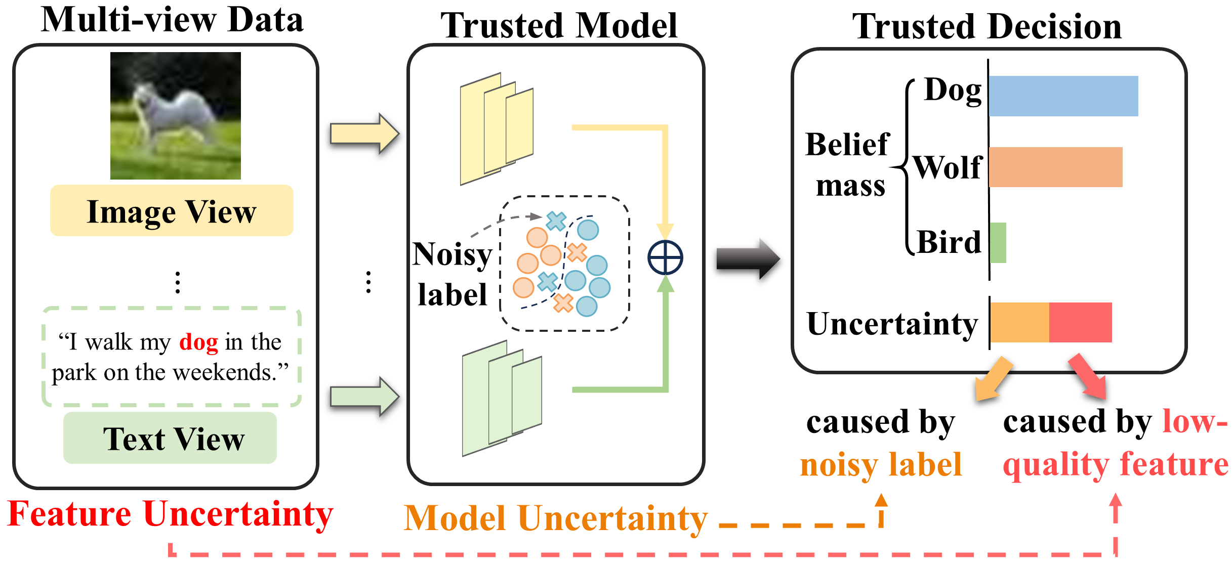
Figure 1: Visualization of the generalized trusted multi-view learning problem: the model should recognize the feature and model uncertainty caused by low-quality feature and noisy label, respectively.

Most existing multi-view learning methods focus on improving decision accuracy while neglecting the decision uncertainty. This significantly limits the application of multi-view learning in safety-critical scenes, such as healthcare. Recently, Han et al. propose a pioneering work Han et al. (2020), Trusted Multi-view Classification (TMC), to solve this problem. TMC calculates and aggregates the evidences of all views from the original data features. It then utilizes these evidences to parameterize the class distribution, which could be used to estimate the class probabilities and uncertainty. To train the entire model, TMC requires the estimated class probabilities to be consistent with the ground-truth labels. Following this line, researchers propose novel evidence aggregation methods, aiming to enhance the reliability and robustness in the presence of feature noise Gan et al. (2021); Qin et al. (2022), conflictive views Xu et al. (2024) and incomplete views Xie et al. (2023) et al.

Regretfully, these trusted multi-view learning methods consistently rely on high-quality ground-truth labels. The labeling task is time-consuming and expensive especially when dealing with large scale datasets, such as user generated multi-modal contents in social media applications. This motivates us to delve into a new Generalized Trusted Multi-view Learning (GTML) problem: how to develop a reliable multi-view learning model under the guidance of noisy labels? This problem encompasses two key objectives: 1) detecting and refining the noisy label during the training stage; 2) recognizing the model’s uncertainty caused by noisy labels. For example, instances belonging to classes like “cat” and “wolf” might exhibit similarities and are prone to being mislabelled. Consequently, the model should exhibit higher decision uncertainty in such cases. An intuitive analogy is an intern animal researcher (model) may not make high-confidence decisions for all animals (instances), but is aware of the cases where a definitive decision is challenging.

In this paper, we propose an Trusted Multi-view Noise Refining (TMNR) method for the GTML problem. We consider the label noises arising from two sources: low-quality data features, such as blurred and incomplete features, and easily-confused classes, such as classes “cat” and “wolf”. Our objective is to leverage multi-view consistent information for noise detection. To achieve this, we first construct the view-specific evidential Deep Neural Networks (DNNs) to learn view-specific evidence, which could be termed as the amount of support to each category collected from data. We then model the view-specific distributions of class probabilities using the Dirichlet distribution, parameterized with view-specific evidence. These distributions allow us to construct opinions, which consist of belief mass vectors and uncertainty estimates. We design view-specific noise correlation matrices to transform the original opinions to the noisy opinions, which aligns with the noisy label. Considering that low-quality data features are prone to mislabeling, we require the diagonal elements of the noise correlation matrices to be inversely proportional to the uncertainty. Additionally, we incorporate class relations into the off-diagonal elements. For instance, the elements corresponding to “cat” and “wolf” should have larger values since these two classes are easily mislabelled. Next, we aggregate the noisy opinions to obtain the common evidence. Finally, we employ a generalized maximum likelihood loss on the common evidence, guided by the noisy labels, for model training.

The main contributions of this work are summarized as follows: 1) we propose the generalized trusted multi-view learning problem, which necessitates the model’s ability to make reliable decisions despite the presence of noisy guidance; 2) we propose the TMNR method to tackle this problem. TMNR mitigates the negative impact of noisy labels through two key strategies: leveraging multi-view consistent information for detecting and refining noisy labels, and assigning higher decision uncertainty to instances belonging to easily mislabelled classes; 3) we empirically compare TMNR with state-of-the-art trusted multi-view learning and label noise learning baselines on 5 publicly available datasets. Experiment results show that TMNR outperforms baseline methods on accuracy, reliability and robustness.

2 Related Work

2.1 Deep Multi-view Fusion

Multi-view fusion has demonstrated its superior performance in various tasks by effectively combining information from multiple sources or modalities Xu et al. (2022); Zhou et al. (2023). According to the fusion strategy, existing deep multi-view fusion methods can be roughly classified into feature fusion Wang et al. (2015); Xu et al. (2022); Lin et al. (2022) and decision fusion Jillani et al. (2020); Liu et al. (2022). A major challenge of feature fusion methods is each view might exhibit different types and different levels of noise at different points in time. Trust decision fusion methods solve this making view-specific trust decisions to obtain the view-specific reliabilities, then assigning large weights to these views with high reliability in the multi-view fusion stage. Following this line, Xie et al. Xie et al. (2023) tackle the challenge of incomplete multi-view classification through a two-stage approach, involving completion and evidential fusion. Xu et al. Xu et al. (2024) focus on making trust decisions for instances that exhibit conflicting information across multiple views. They propose an effective strategy for aggregating conflicting opinions and theoretically prove this strategy can exactly model the relation of multi-view common and view-specific reliabilities. However, it should be noted that these trusted multi-view learning methods heavily rely on high-quality ground-truth labels, which may not always be available or reliable in real-world scenarios. This limitation motivates for us to delve into the problem of GTML, which aims to learn a reliable multi-view learning model under the guidance of noisy labels.

2.2 Label-Noise Learning

In real-world scenarios, the process of labeling data can be error-prone, subjective, or expensive, leading to noisy labels. Label-noise learning refers to the problem of learning from training data that contains noisy labels. In multi-classification tasks, label-noise can be categorized as Class-Conditional Noise (CCN) and Instance-Dependent Noise (IDN). CCN occurs when the label corruption process is independent of the data features, and instances in a class are assigned to other classes with a fixed probability. Dealing with CCN noise often involves correcting losses by estimating an overall category transfer probability matrix Patrini et al. (2017); Hendrycks et al. (2018). IDN refers to instances being mislabeled based on their class and features. In this work, we focus on IDN as it closely resembles real-world noise. The main challenge lies in approximating the complex and high-dimensional instance-dependent transfer matrix. Several approaches have been proposed to address this challenge. For instance, Cheng et al. Cheng et al. (2020) proposes an instance-dependent sample sieve method that enables model to process clean and corrupted samples individually. Cheng et al. Cheng et al. (2022) effectively reduce the complexity of the instance-dependent matrix by streaming embedding. Berthon et al. Berthon et al. (2021) approximate the transfer distributions of each instance using confidence scores. However, the confidence depends on the pre-trained model and may not reliable. The proposed TMNR reliably bootstraps the correlation matrix based on multi-view opinions, leading to superior performance. In addition, TMNR not only refines the noise in the labels but also recognizes the model’s uncertainty caused by noisy labels.

3 The Method

In this section, we first define the generalized trusted multi-view learning problem, then present Trusted Multi-view Noise Refining (TMNR) in detail, together with its implementation.

3.1 Notations and Problem Statement

We use $\{\bm{x}^{v}_{n}\in\mathbb{R}^{d_{v}}\}_{v=1}^{V}$ to denote the feature of the $n$-th instance, which contains $V$ views, $d_{v}$ denotes the dimension of the $v$-th view. $y_{n}\in\{1,...,K\}$ denotes the ground-truth category, where $K$ is the number of all categories. In the generalized trusted multi-view classification problem, the labels of some data instances contain noise as shown in Figure 2. Therefore, we use $\{\tilde{y}_{n}\in\{1,...,K\}\}_{n=1}^{N}$ as the noisy label set that may have been corrupted.

The objective is to learn a trusted classification model according to noisy training instances ${\{\{\bm{x}_{n}^{v}\}_{v=1}^{V}},\tilde{y}_{n}\}_{n=1}^{N_{train}}$. For the instances of the test sets, the model should predict the category $\{{y}_{n}\}$ and uncertainty $\{{u}_{n}\}$, which can quantify the uncertainty caused by low-quality feature and noisy label.

Figure 2: Illustration of the label-noise. Each color represents a ground-truth category $y$.

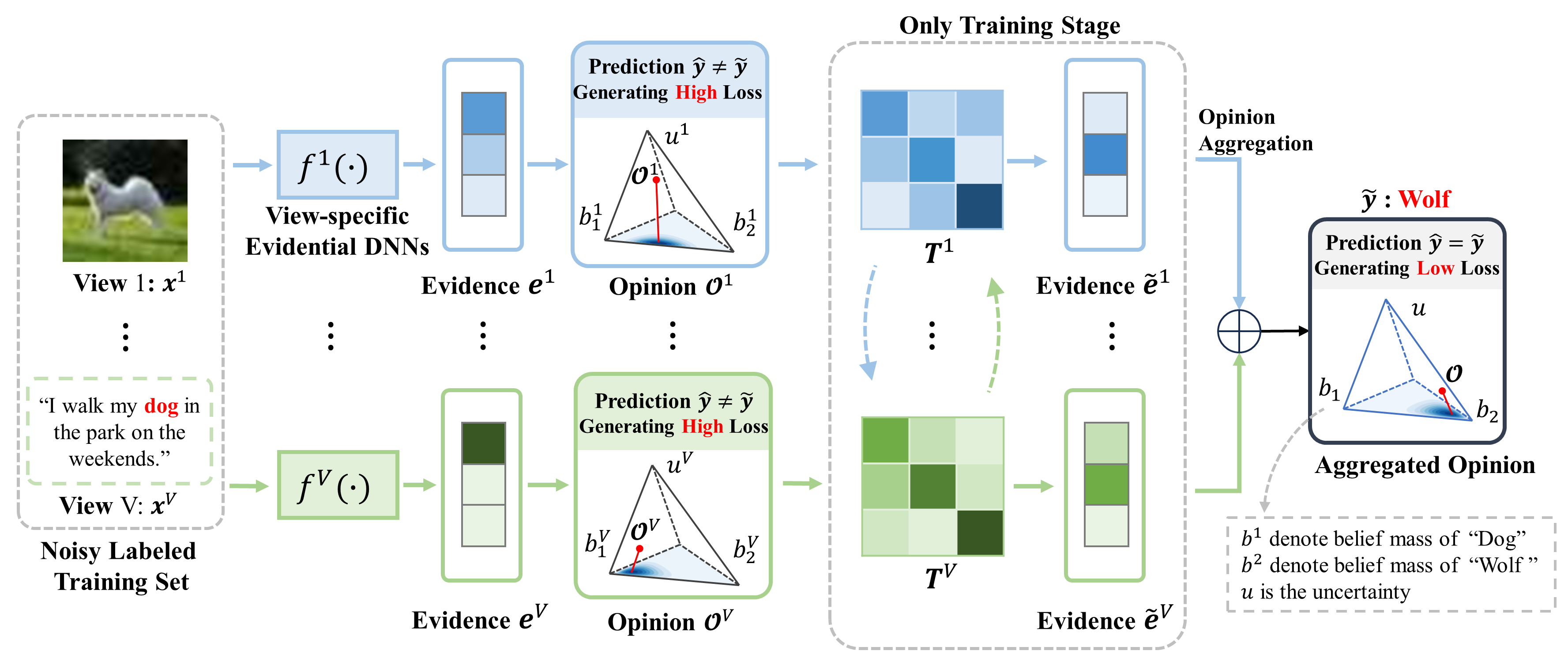
Figure 3: Illustration of TMNR. We first construct view-specific opinions using evidential DNNs $\{f^{v}(\cdot)\}_{v=1}^{V}$. Subsequently, the view-specific noise correlation matrices $\{\bm{T}^{v}\}_{v=1}^{V}$ transform the original opinions into noisy opinions aligned with the noisy labels. Finally, we aggregates the noisy opinions and trains the whole model by the noisy labels.

3.2 Trusted Multi-view Noise Refining Pipeline

As shown in Figure 3, We first construct view-specific opinions using evidential DNNs $\{f^{v}(\cdot)\}_{v=1}^{V}$. To account for the presence of label noise, the view-specific noise correlation matrices $\{T^{v}\}_{v=1}^{V}$ transform the original opinions into noisy opinions aligned with the noisy labels. Finally, we aggregates the noisy opinions and trains the whole model by the noisy labels. Details regarding each component will be elaborated as below.

3.2.1 View-specific Evidence Learning

In this subsection, we introduce the evidence theory to quantify uncertainty. Traditional multi-classification neural networks usually use a Softmax activation function to obtain the probability distribution of the categories. However, this provides only a single-point estimate of the predictive distribution, which can lead to overconfident results even if the predictions are incorrect. This limitation affects the reliability of the results. To address this problem, EDL Sensoy et al. (2018) introduces the evidential framework of subjective logic Jøsang (2016). It converts traditional DNNs into evidential neural networks by making a small change in the activation function to get a non-negative output (e.g.,ReLU) to extract the amount of support (called evidence) for each class.

In this framework, the parameter $\bm{\alpha}$ of the Dirichlet distribution $Dir(\bm{p}|\bm{\alpha})$ is associated with the belief distribution in the framework of evidence theory, where $\bm{p}$ is a simplex representing the probability of class assignment. We collect evidence, $\{\bm{\mathit{e}}_{n}^{v}\}$ by view-specific evidential DNNs $\{f^{v}(\cdot)\}_{v=1}^{V}$. The corresponding Dirichlet distribution parameter is $\bm{\alpha}^{v}=\bm{e}^{v}+1=[\alpha_{1}^{v},\cdots,\alpha_{K}^{v}]^{T}$. After obtaining the distribution parameter, we can calculate the subjective opinion ${\mathcal{O}}^{v}=({\bm{b}^{v},u^{v}})$ of the view including the quality of beliefs $\bm{b}^{v}$ and the quality of uncertainty $u$, where $\bm{b}^{v}=(\bm{\alpha}^{v}-1)/S^{v}=\bm{e}^{v}/S^{v}$, $u^{v}=K/S^{v}$, and $S^{v}=\sum_{k=1}^{K}\alpha_{k}^{v}$ is the Dirichlet intensity.

3.2.2 Evidential Noise Forward Correction

In the GTML problem, we expect to train the evidence network so that its output is a clean evidence distribution about the input. To minimise the negative impact of IDN in the training dataset, we modify the outputs of the DNNs with an additional structure to adjust the loss of each training sample before updating the parameters of the DNNs. This makes the optimisation process immune to label noise, called evidential noise forward correction. This structure should be removed when predicting test data.

For each view $\{\bm{x}^{v}\}_{v=1}^{V}$ of a specific instance, we construct view-specific noise correlation matrix to model the noise process:

$$\bm{T}^{v}=[t_{kj}^{v}]_{k,j=1}^{K}\in[0,1]^{K\times K},$$ (1)

where ${t}_{kj}^{v}:=P(\tilde{y}=j|y=k,\bm{x}^{v})$ and $\sum_{j=1}^{K}t^{v}_{kj}=1$.

To predict probability distributions, the noise class posterior probability is obtained by calculating the correlation matrix:

$$P(\tilde{y}=j|\bm{x}^{v}) =\sum_{k=1}^{K}P(\tilde{y}=j,y=k|\bm{x}^{v})$$

$$=\sum_{k=1}^{K}{t}^{v}_{kj}P(y=k|\bm{x}^{v}).$$ (2)

Based on the evidence theory described in the previous subsection and considering the constraints within $\bm{T}^{v}$ itself, we convert the transfer of predicted probabilities of instances into a transfer of the extracted support at the evidence level using the following equation:

$$\tilde{e}_{j}^{v} =\sum_{k=1}^{K}t_{kj}^{v}\ e_{k}^{v},$$ (3)

where $\tilde{e}_{j}^{v}$/${e}_{k}^{v}$ denotes the $j$-/$k$-th element in the noise/clean class-posterior evidence quantities $\tilde{\bm{e}}^{v}$/${\bm{e}}^{v}$.

Therefore, the clean posterior $\bm{e}^{v}$ obtained from the prediction of each view is transferred to the noisy posterior $\tilde{\bm{e}}^{v}$. The parameter $\tilde{\bm{\alpha}}$ in the noisy Dirichlet distribution is computed in order to align the supervised labels $\tilde{y}$ that contain the noise. The entire evidence vector could be calculabed by:

$$\tilde{\bm{e}}^{v}={\bm{T}^{v}}^{\top}\bm{e}^{v},~{}~{}\tilde{\bm{\alpha}}^{v}=\tilde{\bm{e}}^{v}+1.$$ (4)

3.2.3 Trust Evidential Multi-view Fusion

After obtaining opinions from multiple views, we consider dynamically integrating them based on uncertainty to produce a combined opinion. We achieve this via the Dempster’s combination rule. We take the clean opinion aggregation as example. Given clean opinions of two views of the same instance, i.e., ${\mathcal{O}}^{1}=(\bm{b}^{1},u^{1})$ and ${\mathcal{O}}^{2}=(\bm{b}^{2},u^{2})$, the computation to obtain the aggregated opinion ${\mathcal{O}}=\mathcal{O}^{1}\diamond\mathcal{O}^{2}=(\bm{b},u)$ is defined as follows:

$$b_{k}=\frac{1}{1-C}\left(b_{k}^{1}b_{k}^{2}+b_{k}^{1}u^{2}+b_{k}^{2}u^{1}\right),u=\frac{1}{1-C}u^{1}u^{2},$$ (5)

where $C=\sum_{i\neq j}b_{i}^{1}b_{j}^{2}$.

For a set of opinions from multiple views ${\{\mathcal{O}^{v}\}}_{v=1}^{V}$, the joint multi-view subjective opinion is obtained by $\mathcal{O}=\mathcal{O}^{1}\diamond\mathcal{O}^{2}\diamond\cdots\mathcal{O}^{V}$. The corresponding parameters of the $Dir(\bm{p}|\bm{\alpha})$ are obtained with $S=K/u$, $\alpha_{k}=b_{k}\times S+1$ and the final probability could be estimated via $p_{k}=\alpha_{k}/S$.

3.3 Loss Function

In this section, we explore the optimization of the parameter set $\{\bm{\theta},\bm{\omega}\}$ in the evidence extraction network $f(\cdot;\bm{\theta})$ and the correlation matrices $\{\{\bm{T}_{n}^{v}\}_{v=1}^{V}\}_{n=1}^{N_{train}}$.

3.3.1 Classification loss

We capture view-specific evidence from a single view $\bm{x}^{v}$ of a sample. The vector $\bm{e}^{v}=f^{v}(\bm{x}^{v})$ denotes the clean class-posterior evidence obtained from the corresponding view network prediction. This evidence undergoes correction through Eq. (4) to yield the noisy class-posterior evidence, denoted as $\tilde{\bm{e}}^{v}$, along with the associated Dirichlet parameter $\tilde{\bm{\alpha}}^{v}$. Then in the constructed inference framework, the evidence multi-classification loss $\mathcal{L}$ containing the classification loss $\mathcal{L}_{ace}$ and the Kullback-Leibler (KL) divergence term $\mathcal{L}_{KL}$ is defined, where the classification loss $\mathcal{L}_{ace}$ is obtained by adjusting for the conventional cross-entropy loss, as denoted below:

$$\mathcal{L}_{ace}(\tilde{\bm{\alpha}}^{v})=\sum_{k=1}^{K}\tilde{y}_{k}\left(\psi\left(\tilde{S}^{v}\right)-\psi\left(\tilde{\alpha}_{k}^{v}\right)\right),$$ (6)

where $\psi(\cdot)$ is the digamma function, $\tilde{\alpha}_{j}^{v}$ denote the $j$-th element in $\tilde{\bm{\alpha}}^{v}$.

Eq. (6) does not ensure that the wrong classes in each sample produce lower evidence, and we would like it to be reduced to zero. Thus the KL divergence term is expressed as:

$$\mathcal{L}_{KL}(\tilde{\bm{\alpha}}^{v}) =KL\left[D(\bm{p}^{v}|\bar{\bm{\alpha}}^{v})\parallel D(\bm{p}^{v}|\mathbf{1})\right],$$

where $\bar{\bm{\alpha}}^{v}=\tilde{\mathbf{y}}+(1-\tilde{\mathbf{y}})\odot\tilde{\bm{\alpha}}^{v}$ is the Dirichlet parameter adjusted to remove non-misleading evidence. $\tilde{\mathbf{y}}$ denotes the noisy label $\tilde{y}$ in the form of a one-hot vector, and $\Gamma(\cdot)$ is the gamma function. Thus for a given view’s Dirichlet parameter $\tilde{\bm{\alpha}}^{v}$, the view-specific loss is

$$\mathcal{L}(\tilde{\bm{\alpha}}^{v})=\mathcal{L}_{ace}(\tilde{\bm{\alpha}}^{v})+\lambda\mathcal{L}_{KL}(\tilde{\bm{\alpha}}^{v}),$$ (7)

where $\lambda\in[0,1]$ is a changeable parameter, and we gradually increase its value during training to avoid premature convergence of misclassified instances to a uniform distribution.

3.3.2 Uncertainty-guided correlation loss

Optimizing the view-specific correlation matrix, being a function of the high-dimensional input space, presents challenges without any underlying assumptions. In the context of the IDN problem, it is important to recognize that the probability of a sample being mislabeled depends not only on its category but also on its features. When the features contain noise or are difficult to discern, the likelihood of mislabeling increases significantly. As highlighted earlier, the uncertainty provided by the evidence theory has proven effective in assessing the quality of sample features. Therefore, it is natural for us to combine the uncertainty estimation with the IDN problem, leveraging its potential to enhance the overall performance.

In our work, we do not directly reduce the complexity of correlation matrix by simplifying it. Instead, we propose an assumption that “the higher the uncertainty of the model on the decision, the higher the probability that the sample label is noisy”. Based on this assumption, a mild constraint is imposed on the correlation matrix to effectively reduce the degrees of freedom of its linear system. Specifically, based on the obtained Dirichlet parameters $\tilde{\bm{\alpha}}^{v}$ with its corresponding opinion uncertainty $u^{v}$. We impose different constraints on various parts of the correlation matrix $\bm{T}^{v}$, aiming to encourage it to transfer evidence for instances with higher uncertainty and uncover potential labeling-related patterns.

Diagonal elements. Since the diagonal element $\{t_{kk}^{v}\}_{k=1}^{K}$ in the $\bm{T}^{v}$ corresponds to the probability that the labelled category is equal to its true category. Meanwhile the confidence we obtain from subjective opinions is only relevant for the diagonal elements corresponding to their labelled category $\tilde{y}$, for $\{t_{kk}^{v}\}_{k=1,k\neq\tilde{y}}^{K}$, $u^{v}$ no longer provides any direct information. Therefore, we simply make the other diagonal elements close to the confidence mean of the corresponding class of samples from the current batch. It can be expressed as:

$$\mathcal{M_{D}}(\tilde{\bm{\alpha}}^{v})=\sum_{k=1}^{K}\mathcal{M_{D}}_{k}(\tilde{\bm{\alpha}}^{v}),$$ (8)

$$\mathcal{M_{D}}_{k}(\tilde{\bm{\alpha}}^{v})=\begin{cases}[(1-u^{v})-t_{kk}^{v}]^{2},&\text{if}~{}~{}k=\tilde{y},\\ [(1-\bar{u}_{k}^{v})-t_{kk}^{v}]^{2},&\text{if}~{}~{}k\neq\tilde{y},\end{cases}$$ (9)

where $u^{v}=K/\sum_{k=1}^{K}\tilde{\alpha}_{k}^{v}$ , $\bar{u}_{k}^{v}$ is the average of the $u^{v}$ of all samples with label $\tilde{y}=i$ in the current batch.

Non-diagonal elements. The constraints on the diagonal elements could be regarded as guiding the probability of the sample being mislabeled. The probability of being mislabeled as another category is influenced by the inherent relationship between the different categories. For example, “dog” is more likely to be labeled as “wolf” than as “plane”. Considering that samples in the same class can be easily labeled as the same error class, the transfer probabilities of their non-diagonal elements should be close. In addition, since the labeled information may contain noise, we aim to eliminate the misleading of the error samples in the same class. To solve this problem, we construct the affinity matrix $\{S\}_{v=1}^{V}$ for each viewpoint and calculate this loss with only the $k$ most similar samples in the same class, and for the $n$-th sample:

$$\mathcal{M_{O}}(\tilde{\bm{\alpha}}_{n}^{v})=\sum_{m=1}^{N}s_{nm}^{v}\|\bar{\bm{T}}^{v}_{n}-\bar{\bm{T}}^{v}_{m}\|^{2},$$ (10)

$$s_{mn}^{v}=\left\{\begin{array}[]{ cc}e^{-\frac{||\bm{x}_{m}^{v}-\bm{x}_{n}^{v}||^{2}}{\sigma^{2}}},&\text{if}\ \bm{x}_{m}^{v}\in\mathcal{N}(\bm{x}_{n}^{v},k)\ \text{and}\ \tilde{y}_{n}=\tilde{y}_{m},\\ 0,&\text{else},\end{array}\right.$$ (11)

where $s_{nm}^{v}$ denotes the $(n,m)$-th element in the affinity matrix ${S}^{v}$ for the $v$-th view, which measures the similarity between $\bm{x}_{n}^{v}$ and $\bm{x}_{m}^{v}$. $\mathcal{N}(\bm{x}_{p}^{v},k)$ indicates the $k$-nearest neighbours of the view $\bm{x}_{p}^{v}$. $\bar{\bm{T}}^{v}_{i}$ is the matrix after zeroing the diagonal elements of $\bm{T}^{v}_{i}$. Thus, the overall regularization term for the inter-sample uncertainty bootstrap is expressed as:

$$\mathcal{M}(\tilde{\bm{\alpha}}^{v})=\mathcal{M_{D}}(\tilde{\bm{\alpha}}^{v})+\mathcal{M_{O}}(\tilde{\bm{\alpha}}^{v})$$ (12)

Algorithm 1 TMNR algorithm

/*Training*/
Input: Noisy training dataset, hyperparameter $\beta$, $\gamma$
Output: Parameters of model

1:  Initialize the parameters of the evidence neural network.

2:  Initialise all correlation matrices $\bm{T}$ as unit matrices.

3:  while not converged do

4:     for $v=1:V$ do

5:        Obtain clean evidence $\bm{e}^{v}_{n}$ with $f^{v}(\bm{x}^{v}_{n};\bm{\theta})$;

6:        Obtain $\tilde{\bm{e}}^{v}_{n}$ and $\tilde{\bm{\alpha}}^{v}_{n}$ through Eq. (4);

7:     end for

8:     Aggregation to obtain $\tilde{\bm{\alpha}}_{n}$ by Eq. (5);

9:     Calculate overall loss with Eq. (14);

10:     Update the parameters;

11:     Correct $\bm{T}$ to satisfy Eq. (1).

12:  end while

/*Test*/
Calculate the clean joint $Dir(\bm{p}|\bm{\alpha})$ and the corresponding uncertainty $u$ by $f(\cdot;\bm{\theta})$

Inter-view consistency. In multi-view learning, each view represents different dimensional features of the same instance. In our approach, we leverage the consistency principle of these views to ensure the overall coherence of the correlation matrix across all views. The consistency loss is denoted as:

$$\mathcal{L}_{con}=\frac{1}{V}\sum_{v=1}^{V}\left({\textstyle\sum_{k=1}^{K}}{\textstyle\sum_{j=1}^{K}|t_{kj}^{v}-\bar{t}_{kj}|}\right),$$ (13)

where $\bar{t}_{kj}=(\sum_{v=1}^{V}t_{kj}^{v})/\ V$.

3.3.3 Overall Loss

To sum up, for a multi-view instance $\{\bm{x}^{v}\}^{V}_{v=1}$, to ensure that view-speicfic and aggregated opinions receive supervised guidance. We use a multitasking strategy and bootstrap the correlation matrix according to the designed regularization term:

$$\mathcal{L}_{all}=\mathcal{L}(\tilde{\bm{\alpha}})+\sum_{v=1}^{V}\left[\mathcal{L}\left(\tilde{\bm{\alpha}}^{v}\right)+\beta\left(\mathcal{M}(\tilde{\bm{\alpha}}^{v})\right)\right]+\gamma\mathcal{L}_{con},$$ (14)

where $\beta$ and $\gamma$ are hyperparameters that balances the adjusted cross-entropy loss with the uncertainty bootstrap regularisation and the inter-view consistency loss. ${\tilde{\bm{\alpha}}}$ is obtained by aggregating multiple noise class-posterior parameters $\{\tilde{\bm{\alpha}}^{v}\}_{v=1}^{V}$.

The overall procedure is summarized in Algorithm 1.

4 Experiments

In this section, we test the effectiveness of the proposed method on 5 real-world multi-view datasets with different proportions of labelling noise added. In addition, we also verify the ability of the model to handle low-quality features and noisy label.

4.1 Experimental Setup

Datasets.  UCI contains features for handwritten numerals (’$0$’-’$9$’). The average of pixels in 240 windows, 47 Zernike moments, and 6 morphological features are used as 3 views. PIE consists of 680 face images from 68 experimenters. We extracted 3 views from it: intensity, LBP and Gabor. BBC includes 685 documents from BBC News that can be categorised into 5 categories and are depicted by 4 views. Caltech101 contains 8677 images from 101 categories, extracting features as different views with 6 different methods: Gabor, Wavelet Moments, CENTRIST, HOG, GIST, and LBP. we chose the first 20 categories. Leaves100 consists of 1600 leaf samples from 100 plant species. We extracted shape descriptors, fine-scale edges, and texture histograms as 3 views.

Compared Methods.  (1) Sing-view uncertainty aware methods contain MCDO Gal and Ghahramani (2016) measuring uncertainty by using dropout sampling in both training and inference phases. IEDL Deng et al. (2023) is the SOTA method that involving evidential deep learning and Fisher’s information matrix. (2) Label noise refining methods contain: FC Patrini et al. (2017) corrects the loss function by a CCN transition matrix. ILFC Berthon et al. (2021) explored IDN transition matrix by training a naive model on a subset. (3) Multi-view feature fusion methods contain: DCCAE Wang et al. (2015) train the autoencoder to obtain a common representation between the two views. DCP Lin et al. (2022) is the SOTA method that obtain a consistent representation through dual contrastive loss and dual prediction loss. (4) Multi-view decision fusion methods contain: ETMC Han et al. (2022) estimates uncertainty based on EDL and dynamically fuses the views accordingly to obtain reliable results. ECML Xu et al. (2024) is the SOTA method that propose a new opinion aggregation strategy. We summarize baseline methods in Table 1. For the single-view baselines, we concatenate feature vectors of different views.

Methods	Trusted	Multi-view	Noise Refining
MCDO	✔	✘	✘
IEDL	✔	✘	✘
FC	✘	✘	✔
ILFC	✘	✘	✔
DCCAE	✘	✔	✘
DCP	✘	✔	✘
ETMC	✔	✔	✘
ECML	✔	✔	✘
TMNR	✔	✔	✔

Table 1: Summary of the methods. ✔ denotes the corresponding information is used.

Implementation Details. We implement all methods on PyTorch $1.13$ framework. In our model, the view-specific evidence extracted by fully connected networks with a ReLU layer. The correlation matrices are initially set as unit matrix. We utilize the Adam optimizer with a learning rate of $1e^{-3}$ and $l_{2}$-norm regularization set to $1e^{-5}$. In all datasets, 20% of the instances are split as the test set. We run $5$ times for each method to report the mean values and standard deviations. We follow Cheng et al. (2020) to generate the instance-dependent label noise training sets.

Datasets	Noise	Methods
		MCDO	IEDL	FC	ILFC	DCCAE	DCP	ETMC	ECML	TMNR
UCI	0%	97.50$\pm$0.72	97.70$\pm$0.46	97.05$\pm$0.19	95.50$\pm$0.76	85.75$\pm$0.32	96.15$\pm$0.49	96.20$\pm$0.73	97.05$\pm$0.48	96.90$\pm$0.65
	10%	95.50$\pm$0.61	95.25$\pm$1.25	96.20$\pm$0.58	95.45$\pm$0.82	85.50$\pm$0.70	95.55$\pm$0.54	95.50$\pm$0.33	95.85$\pm$0.19	95.95$\pm$0.37
	20%	95.40$\pm$0.82	95.50$\pm$0.75	95.35$\pm$1.06	95.15$\pm$0.46	85.00$\pm$0.37	95.25$\pm$0.87	95.35$\pm$0.49	95.35$\pm$0.66	95.90$\pm$0.84
	30%	92.30$\pm$0.80	92.50$\pm$1,74	91.90$\pm$1.21	93.85$\pm$1.51	84.50$\pm$0.98	92.40$\pm$1.24	93.15$\pm$1.49	92.85$\pm$1.42	94.00$\pm$1.46
	40%	90.15$\pm$1.44	90.30$\pm$1.99	89.90$\pm$1.58	90.95$\pm$1.87	84.50$\pm$0.78	90.30$\pm$1.08	91.65$\pm$1.54	92.35$\pm$1.37	94.65$\pm$1.35
	50%	83.65$\pm$1.98	85.85$\pm$1.17	83.55$\pm$2.93	84.85$\pm$1.23	81.75$\pm$1.08	83.75$\pm$1.64	84.10$\pm$1.83	86.15$\pm$1.62	88.90$\pm$0.49
PIE	0%	89.71$\pm$3.15	90.85$\pm$3.31	71.03$\pm$5.02	73.28$\pm$3.27	53.38$\pm$1.82	87.24$\pm$2.48	87.06$\pm$2.89	89.83$\pm$2.66	89.53$\pm$ 1.89
	10%	77.50$\pm$3.37	85.74$\pm$4.50	55.00$\pm$3.87	66.44$\pm$4.12	47.06$\pm$0.76	82.70$\pm$3.21	83.38$\pm$1.28	83.09$\pm$3.75	86.47$\pm$1.97
	20%	64.71$\pm$1.40	80.29$\pm$3.58	44.85$\pm$4.05	61.23$\pm$3.21	47.79$\pm$1.87	75.76$\pm$1.84	77.21$\pm$1.04	76.47$\pm$1.54	83.24$\pm$1.70
	30%	55.44$\pm$3.28	69.44$\pm$2.73	33.97$\pm$1.94	58.98$\pm$4.10	36.03$\pm$0.67	65.38$\pm$2.49	63.97$\pm$1.86	70.44$\pm$4.04	73.29$\pm$2.08
	40%	46.32$\pm$2.03	65.29$\pm$4.57	32.31$\pm$5.29	51.84$\pm$5.29	33.82$\pm$1.19	58.46$\pm$2.96	61.76$\pm$2.33	63.97$\pm$4.53	71.91$\pm$2.33
	50%	38.68$\pm$3.50	53.00$\pm$2.88	25.44$\pm$2.57	44.02$\pm$4.23	30.88$\pm$1.38	50.85$\pm$2.82	51.32$\pm$3.40	55.53$\pm$2.30	59.85$\pm$2.89
BBC	0%	93.31$\pm$1.79	92.60$\pm$2.04	92.12$\pm$3.01	92.56$\pm$1.87	92.03$\pm$2.48	93.20$\pm$1.92	93.58$\pm$1.42	91.82$\pm$1.93	93.51$\pm$1.35
	10%	89.34$\pm$1.88	90.38$\pm$1.81	89.41$\pm$1.57	88.28$\pm$1.34	88.24$\pm$1.54	88.33$\pm$1.41	89.93$\pm$1.56	88.18$\pm$1.17	90.07$\pm$1.53
	20%	86.01$\pm$2.86	86.93$\pm$1.87	85.11$\pm$2.47	86.01$\pm$2.02	85.41$\pm$2.97	86.17$\pm$2.38	86.86$\pm$2.73	85.11$\pm$2.87	87.45$\pm$2.86
	30%	74.45$\pm$4.05	81.07$\pm$3.56	73.87$\pm$5.66	77.23$\pm$2.98	77.94$\pm$2.36	77.80$\pm$2.49	80.73$\pm$2.47	74.16$\pm$1.27	82.04$\pm$2.98
	40%	69.64$\pm$2.72	71.06$\pm$1.07	70.51$\pm$1.76	72.67$\pm$3.88	71.09$\pm$2.51	70.87$\pm$3.01	72.85$\pm$3.36	72.85$\pm$3.96	75.91$\pm$3.44
	50%	56.64$\pm$3.59	59.04$\pm$4.52	56.93$\pm$2.44	57.29$\pm$3.90	56.27$\pm$3.87	56.24$\pm$3.76	57.23$\pm$4.30	58.83$\pm$3.05	63.88$\pm$4.43
Caltech101	0%	71.38$\pm$5.06	92.35$\pm$1.46	64.64$\pm$5.57	85.24$\pm$1.90	88.03$\pm$0.75	91.93$\pm$1.39	92.59$\pm$0.86	91.13$\pm$1.61	91.84$\pm$1.08
	10%	68.66$\pm$5.02	91.05$\pm$1.26	57.28$\pm$3.46	81.92$\pm$2.39	86.19$\pm$0.98	90.74$\pm$1.22	90.34$\pm$1.32	91.38$\pm$1.59	91.09$\pm$0.59
	20%	58.41$\pm$2.43	86.82$\pm$2.22	42.34$\pm$5.38	77.74$\pm$2.80	83.47$\pm$1.28	87.02$\pm$2.31	87.74$\pm$1.24	87.12$\pm$0.96	87.78$\pm$1.26
	30%	54.60$\pm$3.58	83.01$\pm$0.90	52.97$\pm$2.54	73.26$\pm$2.11	82.85$\pm$0.93	84.98$\pm$1.01	86.07$\pm$1.10	86.11$\pm$0.49	86.82$\pm$0.83
	40%	48.12$\pm$5.99	71.92$\pm$1.95	46.57$\pm$4.77	70.17$\pm$3.98	75.94$\pm$1.89	76.90$\pm$1.55	78.91$\pm$0.90	77.82$\pm$0.68	81.59$\pm$0.96
	50%	43.89$\pm$6.41	59.04$\pm$1.84	35.98$\pm$4.78	63.28$\pm$3.41	61.09$\pm$1.46	65.29$\pm$2.52	68.79$\pm$2.02	68.91$\pm$1.96	72.89$\pm$1.97
Leaves100	0%	66.12$\pm$5.05	72.12$\pm$0.71	64.06$\pm$4.40	66.27$\pm$3.11	63.50$\pm$0.75	73.40$\pm$2.18	70.62$\pm$3.46	73.00$\pm$1.73	73.75$\pm$2.55
	10%	63.81$\pm$2.87	65.38$\pm$2.18	62.00$\pm$3.38	63.02$\pm$2.94	62.19$\pm$0.97	66.16$\pm$2.47	66.31$\pm$3.16	68.31$\pm$1.45	68.88$\pm$2.17
	20%	60.06$\pm$3.23	63.38$\pm$1.67	59.63$\pm$2.04	59.61$\pm$3.20	61.25$\pm$1.24	61.30$\pm$3.98	59.31$\pm$3.16	62.56$\pm$4.67	64.19$\pm$2.03
	30%	55.31$\pm$4.19	57.37$\pm$3.44	52.62$\pm$3.47	54.75$\pm$3.59	58.13$\pm$0.76	57.44$\pm$2.80	58.75$\pm$1.95	59.94$\pm$5.61	60.94$\pm$2.04
	40%	47.69$\pm$2.26	52.88$\pm$1.39	44.31$\pm$2.59	48.57$\pm$2.16	55.13$\pm$1.87	52.59$\pm$1.97	51.69$\pm$2.27	54.69$\pm$3.89	57.75$\pm$2.12
	50%	40.88$\pm$3.80	48.31$\pm$2.11	36.44$\pm$3.12	40.35$\pm$3.82	50.31$\pm$1.89	49.67$\pm$3.24	51.81$\pm$1.76	50.44$\pm$3.10	55.63$\pm$2.91

Table 2: Classification accuracy($\%$) of TMNR and baseline methods on the datasets with different proportions of Instance-Dependent Noise. The ‘Noise’ column shows the percentage of noisy labelled instances, where $0\%$ denote clean datasets. The best and the second best results are highlighted by boldface and underlined respectively.

4.2 Experimental Results

Performance comparison. The comparison between TMNR and baselines on clean and noisy datasets are shown in Table 2. We can observe the following points: (1) On the clean training dataset, TMNR achieves performance comparable to state-of-the-art methods. This finding indicates that the noise forward correction module has minimal negtive impact on the model’s performance. (2) The performance of multi-view feature fusion methods degrade clearly with the noise ratio increase. The reason is the feature fusion would badly affected by noisy labels. (3) On the noisy training dataset, especially with high noise ratio, TMNR significantly outperforms all baseline. Such performance is a powerful evidence that our proposed method effectively reduces the effect of noisy labels through forward correction. We would further verify this in ablation study and uncertainty evaluation experiments.

Model uncertainty evaluation.  In real-world datasets, various categories have varying probabilities of being labeled incorrectly. If we can identify the classes that are more likely to be labeled incorrectly during the labeling process, we can apply specialized processing to address these classes, such as involving experts in secondary labeling. As incorrect labeling leads to increased model uncertainty, our model can effectively identify classes that contain noise by assessing their predicted uncertainty.

To observe significant results, we intentionally flipped the labels of samples belonging to classes ‘0’ and ‘1’, as well as classes ‘8’ and ‘9’, within the UCI dataset during training. Subsequently, predictions were made on the test samples, and the average uncertainty for each category was calculated. The results, depicted in Figure 4(a), demonstrate a notable increase in uncertainty for the categories where the labels were corrupted. Figure 4(b) presents a heat map displaying the mean values of all trained correlation matrix parameters. The results clearly illustrate that the model’s structure captures the probability of changes in inter-class evidence.

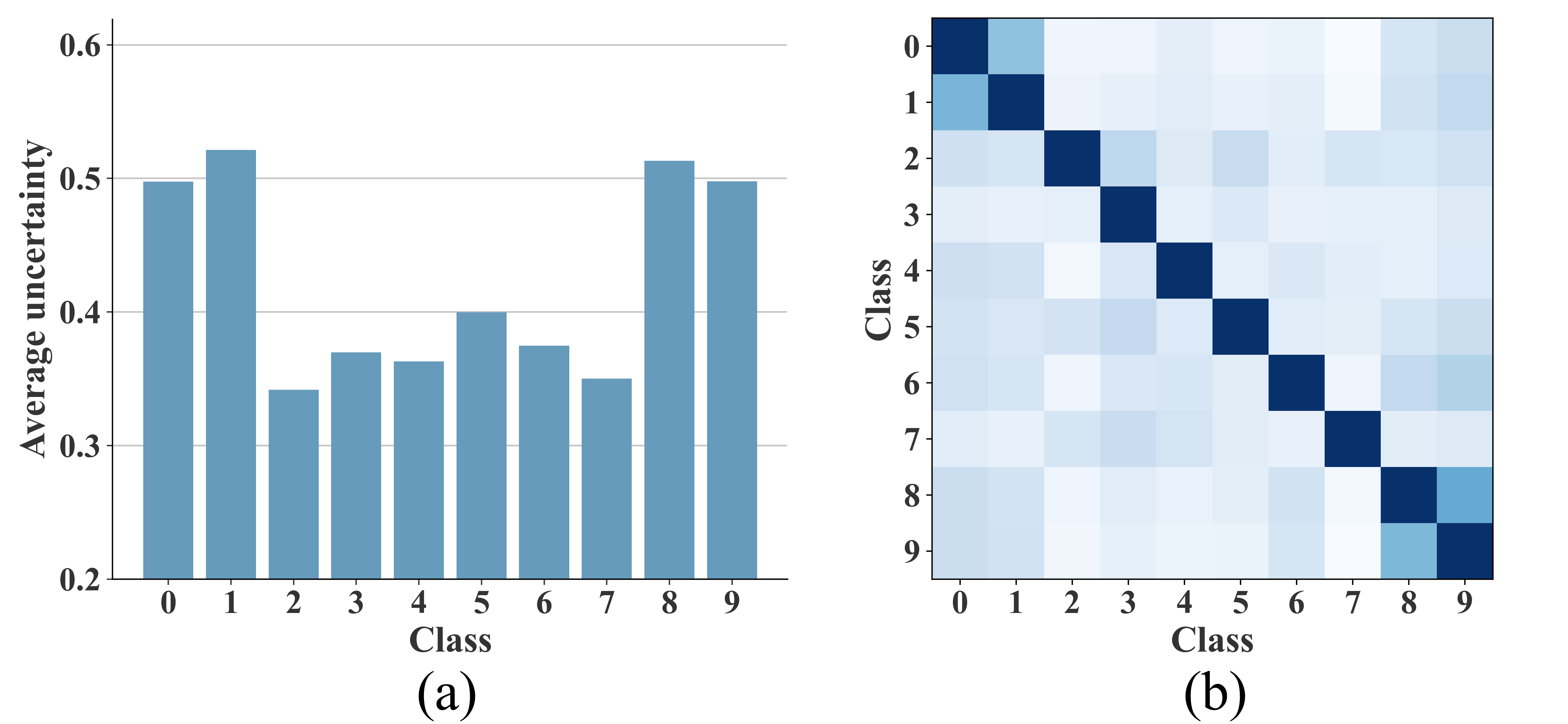
Figure 4: Visualization of the average uncertainty of each category and the correlation matrices.

Correlation matrix evaluation.  We analyze the sensitivity of hyperparameter $\beta$ on all datasets containing 30% noise. The results is shown in Figure 5. It is evident that the sensitivity of the parameter $\beta$ varies across different datasets, yet optimal performance is consistently achieved within the range of 0.05 to 0.1. This observation validates the effectiveness of the regularization applied to the diagonal elements of the correlation matrices. Taking this into consideration, we have determined the appropriate value of $\beta$ for the remaining evaluation experiments.

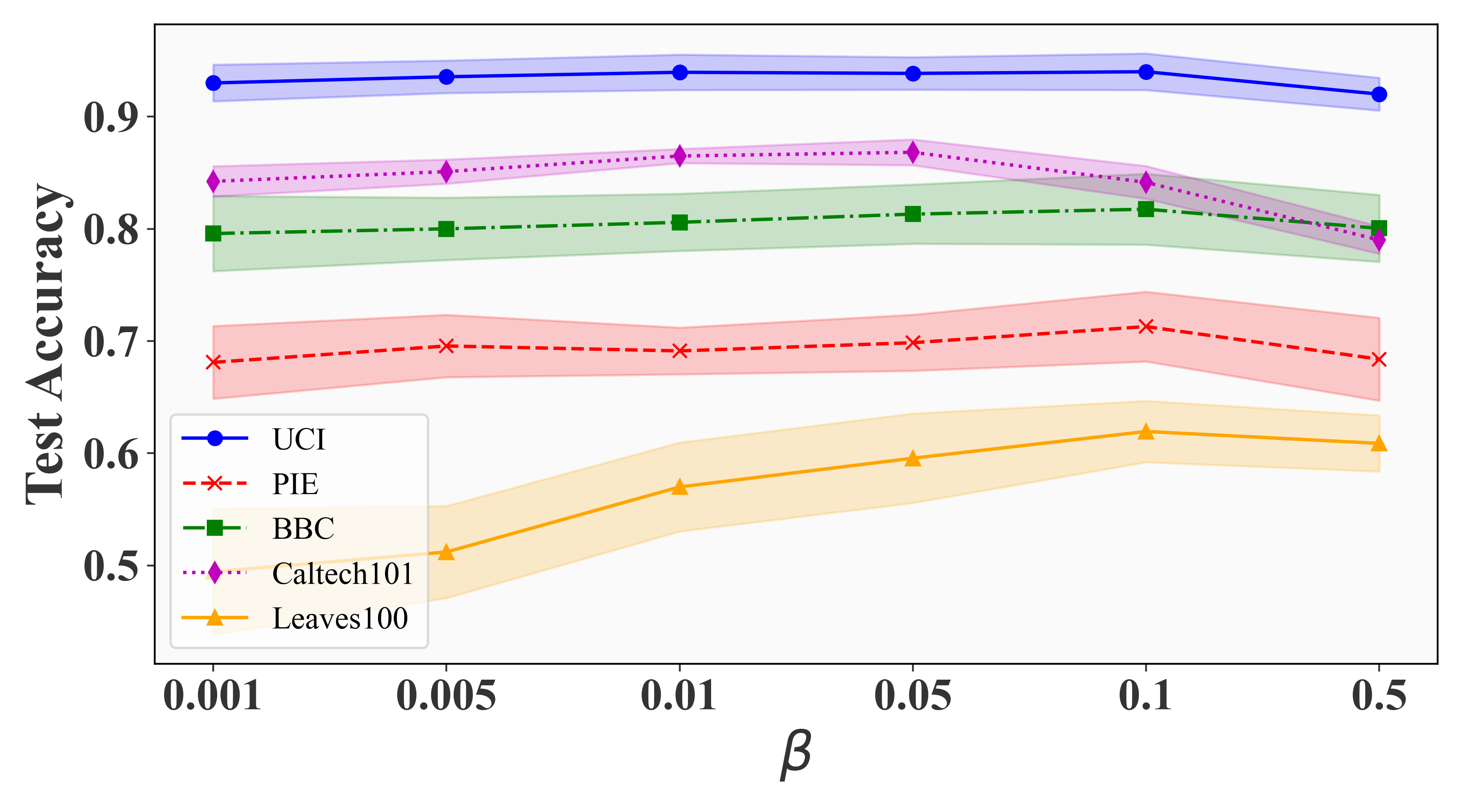
Figure 5: Correlation matrix evaluation. Classification accuracy when adjusting $\bm{\beta}$ on all datasets with 30% noise rate.

5 Conclusion

In this paper, we introduced a TMNR method for addressing the generalized trusted multi-view learning problem. TMNR leverages evidential deep neural networks to learn view-specific belief mass vectors and uncertainty estimates. We further designed view-specific noise correlation matrices to effectively correlate the original opinions with the noisy opinions. By aggregating the noisy opinions and training the entire model using the noisy labels, we achieved robust model training. Experimental results on five real-world datasets validated the effectiveness of TMNR, demonstrating its superiority compared to state-of-the-art baseline methods.

References

- Berthon et al. [2021] Antonin Berthon, Bo Han, Gang Niu, Tongliang Liu, and Masashi Sugiyama. Confidence scores make instance-dependent label-noise learning possible. In International conference on machine learning, pages 825–836. PMLR, 2021.
- Cheng et al. [2020] Hao Cheng, Zhaowei Zhu, Xingyu Li, Yifei Gong, Xing Sun, and Yang Liu. Learning with instance-dependent label noise: A sample sieve approach. In International Conference on Learning Representations, 2020.
- Cheng et al. [2022] De Cheng, Tongliang Liu, Yixiong Ning, Nannan Wang, Bo Han, Gang Niu, Xinbo Gao, and Masashi Sugiyama. Instance-dependent label-noise learning with manifold-regularized transition matrix estimation. In Proceedings of the IEEE/CVF Conference on Computer Vision and Pattern Recognition, pages 16630–16639, 2022.
- Deng et al. [2023] Danruo Deng, Guangyong Chen, Yang Yu, Furui Liu, and Pheng-Ann Heng. Uncertainty estimation by fisher information-based evidential deep learning. In Proceedings of the 40th International Conference on Machine Learning, ICML’23. JMLR.org, 2023.
- Gal and Ghahramani [2016] Yarin Gal and Zoubin Ghahramani. Dropout as a bayesian approximation: Representing model uncertainty in deep learning. In Proceedings of the 33rd International Conference on International Conference on Machine Learning - Volume 48, ICML’16, page 1050–1059. JMLR.org, 2016.
- Gan et al. [2021] Jiangzhang Gan, Ziwen Peng, Xiaofeng Zhu, Rongyao Hu, Junbo Ma, and Guorong Wu. Brain functional connectivity analysis based on multi-graph fusion. Medical image analysis, 71:102057, 2021.
- Han et al. [2020] Zongbo Han, Changqing Zhang, Huazhu Fu, and Joey Tianyi Zhou. Trusted multi-view classification. In International Conference on Learning Representations, 2020.
- Han et al. [2022] Zongbo Han, Changqing Zhang, Huazhu Fu, and Joey Tianyi Zhou. Trusted multi-view classification with dynamic evidential fusion. IEEE transactions on pattern analysis and machine intelligence, 45(2):2551–2566, 2022.
- Hendrycks et al. [2018] Dan Hendrycks, Mantas Mazeika, Duncan Wilson, and Kevin Gimpel. Using trusted data to train deep networks on labels corrupted by severe noise. Advances in neural information processing systems, 31, 2018.
- Huang et al. [2022] Shudong Huang, Yixi Liu, Ivor W Tsang, Zenglin Xu, and Jiancheng Lv. Multi-view subspace clustering by joint measuring of consistency and diversity. IEEE Transactions on Knowledge and Data Engineering, 2022.
- Jillani et al. [2020] Rashad Jillani, Syed Fawad Hussain, and Hari Kalva. Multi-view clustering for fast intra mode decision in hevc. In 2020 IEEE International Conference on Consumer Electronics (ICCE), pages 1–4. IEEE, 2020.
- Jøsang [2016] Audun Jøsang. Subjective logic: A formalism for reasoning under uncertainty. Springer, 2016.
- Liang et al. [2021] Xinyan Liang, Yuhua Qian, Qian Guo, Honghong Cheng, and Jiye Liang. Af: An association-based fusion method for multi-modal classification. IEEE Transactions on Pattern Analysis and Machine Intelligence, 44(12):9236–9254, 2021.
- Lin et al. [2022] Yijie Lin, Yuanbiao Gou, Xiaotian Liu, Jinfeng Bai, Jiancheng Lv, and Xi Peng. Dual contrastive prediction for incomplete multi-view representation learning. IEEE Transactions on Pattern Analysis and Machine Intelligence, 45(4):4447–4461, 2022.
- Lin et al. [2023] Zhenghong Lin, Yanchao Tan, Yunfei Zhan, Weiming Liu, Fan Wang, Chaochao Chen, Shiping Wang, and Carl Yang. Contrastive intra-and inter-modality generation for enhancing incomplete multimedia recommendation. In Proceedings of the 31st ACM International Conference on Multimedia, pages 6234–6242, 2023.
- Liu et al. [2022] Wei Liu, Xiaodong Yue, Yufei Chen, and Thierry Denoeux. Trusted multi-view deep learning with opinion aggregation. In Proceedings of the AAAI Conference on Artificial Intelligence, volume 36, pages 7585–7593, 2022.
- Min et al. [2023] Bonan Min, Hayley Ross, Elior Sulem, Amir Pouran Ben Veyseh, Thien Huu Nguyen, Oscar Sainz, Eneko Agirre, Ilana Heintz, and Dan Roth. Recent advances in natural language processing via large pre-trained language models: A survey. ACM Computing Surveys, 56(2):1–40, 2023.
- Nikzad-Khasmakhia et al. [2020] N Nikzad-Khasmakhia, M Balafara, M Reza Feizi-Derakhshia, and Cina Motamedb. Berters: Multimodal representation learning for expert recommendation system with transformer. arXiv preprint arXiv:2007.07229, 2020.
- Patrini et al. [2017] Giorgio Patrini, Alessandro Rozza, Aditya Krishna Menon, Richard Nock, and Lizhen Qu. Making deep neural networks robust to label noise: A loss correction approach. In Proceedings of the IEEE conference on computer vision and pattern recognition, pages 1944–1952, 2017.
- Qin et al. [2022] Yang Qin, Dezhong Peng, Xi Peng, Xu Wang, and Peng Hu. Deep evidential learning with noisy correspondence for cross-modal retrieval. In Proceedings of the 30th ACM International Conference on Multimedia, pages 4948–4956, 2022.
- Sensoy et al. [2018] Murat Sensoy, Lance Kaplan, and Melih Kandemir. Evidential deep learning to quantify classification uncertainty. Advances in neural information processing systems, 31, 2018.
- Wang et al. [2015] Weiran Wang, Raman Arora, Karen Livescu, and Jeff Bilmes. On deep multi-view representation learning. In International conference on machine learning, pages 1083–1092. PMLR, 2015.
- Xie et al. [2023] Mengyao Xie, Zongbo Han, Changqing Zhang, Yichen Bai, and Qinghua Hu. Exploring and exploiting uncertainty for incomplete multi-view classification. In Proceedings of the IEEE/CVF Conference on Computer Vision and Pattern Recognition, pages 19873–19882, 2023.
- Xu et al. [2022] Lei Xu, Hui Wu, Chunming He, Jun Wang, Changqing Zhang, Feiping Nie, and Lei Chen. Multi-modal sequence learning for alzheimer’s disease progression prediction with incomplete variable-length longitudinal data. Medical Image Analysis, 82:102643, 2022.
- Xu et al. [2023] Jie Xu, Yazhou Ren, Xiaoshuang Shi, Heng Tao Shen, and Xiaofeng Zhu. Untie: Clustering analysis with disentanglement in multi-view information fusion. Information Fusion, 100:101937, 2023.
- Xu et al. [2024] Cai Xu, Jiajun Si, Ziyu Guan, Wei Zhao, Yue Wu, and Xiyue Gao. Reliable conflictive multi-view learning. In Proceedings of the AAAI Conference on Artificial Intelligence, 2024.
- Zhou et al. [2023] Hai Zhou, Zhe Xue, Ying Liu, Boang Li, Junping Du, Meiyu Liang, and Yuankai Qi. Calm: An enhanced encoding and confidence evaluating framework for trustworthy multi-view learning. In Proceedings of the 31st ACM International Conference on Multimedia, pages 3108–3116, 2023.