A variational discretization method for mean curvature flows by the Onsager principle

Abstract

The mean curvature flow describes the evolution of a surface(a curve) with normal velocity proportional to the local mean curvature. It has many applications in mathematics, science and engineering. In this paper, we develop a numerical method for mean curvature flows by using the Onsager principle as an approximation tool. We first show that the mean curvature flow can be derived naturally from the Onsager variational principle. Then we consider a piecewisely linear approximation of the curve and derive a discrete geometric flow. The discrete flow is described by a system of ordinary differential equations for the nodes of the discrete curve. We prove that the discrete system preserve the energy dissipation structure in the framework of the Onsager principle and this implies the energy decreasing property. The ODE system can be solved by an improved Euler scheme and this leads to an efficient fully discrete scheme. We first consider the method for a simple mean curvature flow and then extend it to volume preserving mean curvature flow and also a wetting problem on substrates. Numerical examples show that the method has optimal convergence rate and works well for all the three problems.

1 Introduction

Mean curvature flow describes the process of surface evolution, where a surface moves in its normal direction with a velocity equal to its mean curvature, i.e.

$$\vec{v}=-H\vec{n},$$ (1)

where $\vec{v}$ denotes the velocity of motion of the surface, and $H$ denotes the mean curvature of the surface. $\vec{n}$ is the unit normal vector of the surface. The mean curvature flow first appeared in materials science in the 1920s, and the general mathematical model was first proposed in 1957 in [mullins1957theory], where Mullins used it to describe how grooves develop on the surfaces of hot polycrystals. The mean curvature flow has found numerous applications. One is in image smoothing, where it is used to improve image quality by removing unnecessary noise and enhancing specific features without altering the transmitted information [gallagher2020curve]. Additionally, the mean curvature flow has been employed to model a special form of the reaction-diffusion equation in chemical reactions [rubinstein1989fast].

The numerical approximation of mean curvature flow originates from the pioneering work of Dziuk in 1990 [dziuk1990algorithm]. He proposed a parametric finite element method (PFEM) to solve the problem based on the observation that the mean curvature flow is a diffusion equation for the surface embedding in a bulk region. However, as the surface evolves, the nodes in the PFEMs may overlap, leading to mesh distortion [hu2022evolving]. Subsequently, various techniques have been introduced in PFEMs that allow points on interpolated curves or surfaces to shift tangentially to produce a better distribution of nodes. For example, Deckelnick and Dziuk introduced an artificial tangential velocity in their work [deckelnick1995approximation]. By similar motivation, Elliott and Fritz employed a DeTurck’s trick to introduce a tangential velocity [m2017approximations]. A widely used method is the parametric finite element method developed by Barrett, Garcke, and Nürnberg [barrett2007variational, Barrett2008OnTP, Barrett2008ParametricAO]. They utilize a different variational form which can induce tangential velocity for the mesh nodes automatically. The method have been generalized some other geometrical flows [Barrett2010NumericalAO, barrett2011approximation, barrett2012parametric, jiang2021perimeter, bao2021structure, li2021energy, bao2022volume, bao2023symmetrized, hu2022evolving]. Recently, there are significant progresses in rigorous convergence analysis for discrete schemes for mean curvature flows and some other geometric flows [kovacs2019convergent, kovacs2021convergent, li2020convergence, li2021convergence, Bai2023].

In this paper, we develop a new finite element method for mean curvature flow by using the Onsager principle as an approximation tool. We consider three different problems, namely the standard mean curvature flow, the volume conserving mean curvature flow and a wetting problem with contact with substrate. We show that the dynamic equations of all the three problems can be derived naturally by the Onsager principle. Furthermore, by considering piecewisely linear approximation of the surface, we can derive semi-discrete problems which preserve the energy dissipation relations just as the continuous problems. The discrete volume can also be preserved if the continuous problem preserve the volume. The semi-discrete problems can be further discretized in time by an improved Euler scheme. Numerical examples show that the method works well for all the three problems. In particular, it has optimal convergence rate in space for a mean curvature flow with analytic solutions.

For simplicity in presentation, we consider only two dimensional problems in the paper. However, the method can be generalized to higher dimensional problems straightforwardly. The structure of the paper is as follows. In Section 2, we introduce the main idea to use the Onsager variational principle as an approximation tool. In Section 3, we first derive a continuous partial differential equation for a simple smooth closed curve under mean curvature flow using the Onsager principle. Subsequently, we discretize the equation using piecewisely linear curves and prove the discrete energy decays property. We introduce a penalty term to the energy functional to avoid mesh distortion. In Section 4, we further consider a mean curvature flow with the constraint of volume conservation. We derive a continuity equation and also a discrete problem. In Section 5, we further generalize the method to solve a wetting problem, which is a non-closed curve contacting with substrates. In Section 6, we present several numerical examples to demonstrate the efficiency of the methods. We give a few conclusion remarks in the final section.

2 The Onsager principle as an approximation tool

Consider a physical system which is described by a time-dependent function $u(t)$. For simplication in notation, we denote the time derivative of $u$ by $\dot{u}=\frac{\partial u}{\partial t}$. In a dissipative system, the evolution of $u$ over time may cause energy dissipation, which can be quantified by a dissipation function denoted by $\Phi(\dot{u})$. In many applications, the dissipation function can be expressed as

$$\Phi(\dot{u})=\frac{\xi}{2}\left\|{\dot{u}}\right\|_{2}^{2},$$ (2)

where $\xi$ is a positive friction coefficient. Suppose the free energy of the system is given by a function $\mathcal{E}(u)$. Given $\dot{u}$, the changing rate of the total energy can be computed as

$$\dot{\mathcal{E}}(u;\dot{u})=\langle\frac{\delta\mathcal{E}(u)}{\delta u},\dot{u}\rangle=\left.\frac{\text{d}\mathcal{E}(u+\lambda\dot{u})}{\text{d}\lambda}\right|_{\lambda=0}.$$ (3)

Then we can define a Rayleighian functional as follows

$$\mathcal{R}(u;\dot{u})=\Phi(\dot{u})+\dot{\mathcal{E}}(u;\dot{u}).$$ (4)

Based on the above aforementioned definitions, the Onsager variational principle can be stated as follows [Onsager1931, Onsager1931a, DoiSoft]. For any dissipative system without inertial effect, the evolution of the system can be obtained by minimizing the Rayleighian with respect to $\dot{u}$. In other words, the evolution equation of $u$ is obtained by

$$\min_{\dot{u}\in V}\mathcal{R}(u,\dot{u}),$$ (5)

where $V$ represents the admissible space of $\dot{u}$. Since the Rayleighian is a quadratic form with respect to $\dot{u}$, the minimization problem (5) can be described by the Euler-Lagrange equation

$$(\xi\dot{u},\varphi)=-\langle\frac{\delta\mathcal{E}(u)}{\delta u},\varphi\rangle,\quad\forall\varphi\in V,$$ (6)

or in a simple form

$$\xi\dot{u}=-\frac{\delta\mathcal{E}(u)}{\delta u}.$$ (7)

In physics, this equation implies a balance between the frictional force $-\xi\dot{u}$ and the driven force $\frac{\delta\mathcal{E}(u)}{\delta u}$. For a more comprehensive introduction of the Onsager principle, we refer to [DoiSoft].

Recently, the Onsager principle is used to derive an approximate model for a physical system [Doi2015]. The key idea is follows. Suppose that the system can be described by a system of slow variables $\mathbf{a}=(a_{1},a_{2},\cdots,a_{N})$. Suppose we can compute the approximate energy $\mathcal{E}_{h}(\mathbf{a})$ and the approximate dissipation function $\Phi_{h}(\dot{\mathbf{a}})$. Then we can derive a discrete ODE system by the Onsager principle, which is given by

$$\frac{\delta\Phi_{h}}{\delta\dot{\mathbf{a}}}+\frac{\delta\mathcal{E}_{h}}{\delta\mathbf{a}}=0.$$

The method has been used to develop reduced models in complicated two-phase flows [XuXianmin2016, DiYana2016], some soft matter problems [ManXingkun2016, ZhouJiajia2017], solid dewetting [Jiang19b], and also in dislocation dynamics [dai2021boundary]. It can also be used to derive numerical method for wetting problems [lu2021efficient]. In this following, we will investigate the application of the Onsager principle in deriving numerical schemes for mean curvature flows.

3 Mean curvature flow

3.1 Derivation of the continuous equation by the Onsager principle

For simplicity in presentation, we consider only the two dimensional case. For a simple smooth closed curve $\Gamma(t)$ in the plane, the points on it are denoted by $\vec{x}(t)$. We aim to derive the mean curvature flow equation of $\Gamma(t)$ by using the Onsager variational principle.

First, suppose the dimensionless surface energy in a physical system is given by

$$\mathcal{E}=\int_{\Gamma(t)}\text{d}s=|\Gamma(t)|,$$ (8)

where $s$ is the arc length parameter. In order to calculate the changing rate of the surface energy with respect to time, we need to employ the following Reynolds transport equation for a closed curve [Niven2018RethinkingTR]

$$\frac{\text{d}}{\text{d}t}\int_{\Gamma(t)}f\text{d}s=\int_{\Gamma(t)}[\frac{\partial f}{\partial t}+\nabla_{\Gamma}\cdot(f\vec{v})]\text{d}s=\int_{\Gamma(t)}(\frac{\text{d}f}{\text{d}t}+f\cdot\kappa v_{n})\text{d}s.$$ (9)

Where $\vec{v}=\frac{\text{d}\vec{x}}{\text{d}t}$, $v_{n}=\vec{v}\cdot\vec{n}$ is the normal velocity, and $\kappa$ denotes the curvature of $\Gamma(t)$. Let $f=1$ in (9), we obtain the changing rate of the total energy with respect to time

$$\dot{\mathcal{E}}=\frac{\text{d}}{\text{d}t}\int_{\Gamma(t)}\text{d}s=\int_{\Gamma(t)}\kappa v_{n}\text{d}s.$$ (10)

Suppose that the dissipation function in the system is given by

$$\Phi=\frac{1}{2}\int_{\Gamma(t)}v_{n}^{2}\text{d}s.$$ (11)

Then the corresponding Rayleighian is defined as

$$\mathcal{R}=\Phi+\dot{\mathcal{E}}=\int_{\Gamma(t)}(\frac{1}{2}v_{n}^{2}+\kappa v_{n})\text{d}s.$$ (12)

Using the Onsager principle, we minimize the Rayleighian $\mathcal{R}$ with respect to $v_{n}$, i.e.

$$\min_{v_{n}}\mathcal{R}.$$ (13)

The corresponding Euler-Lagrange equation is

$$v_{n}+\kappa=0.$$ (14)

Substituting the equation (14) into (10), we have

$$\dot{\mathcal{E}}=\int_{\Gamma(t)}\kappa v_{n}\text{d}s=-\int_{\Gamma(t)}\kappa^{2}\text{d}s=-2\Phi(v_{n})\leq 0,$$ (15)

and the equality holds if and only if $\kappa=0$. This implies that the total energy decreases with respect to time for mean curvature flow.

Since the tangential velocity of the curve solely influences the distribution of points along the curve, rather than its shape, the mean curvature flow given by (14) is equivalent to the following equation [LiBuyang2022]

$$\vec{v}=-\kappa\vec{n}.$$ (16)

3.2 A discrete mean curvature flow by the Onsager principle

In this section, we aim to numerically solve the dynamic equation (14). Suppose that the curve $\Gamma(t)$ can be approximated by piecewise linear segments, as illustrated in Figure 1. Denote the nodes by

$$\vec{x}_{1}(t),\vec{x}_{2}(t),...,\vec{x}_{n}(t),$$ (17)

where $\vec{x}_{i}(t)=(x_{i}^{(1)}(t),x_{i}^{(2)}(t))^{T}\ (1\leq i\leq n)$. The line segments connecting adjacent nodes are denoted by $\Gamma_{i}(t)=\overline{\vec{x}_{i}(t)\vec{x}_{i+1}(t)}\ (1\leq i\leq n-1)$ and $\Gamma_{n}(t)=\overline{\vec{x}_{n}(t)\vec{x}_{1}(t)}$. Therefore, the approximate curve is given by $\Gamma_{h}(t)=\bigcup\limits_{i=1}^{n}\Gamma_{i}(t)$.

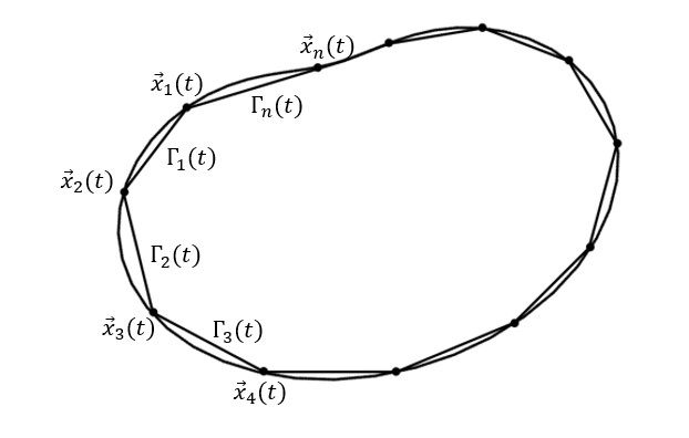
Figure 1: Selection of interpolation points

We will derive the dynamic equation for $\Gamma_{h}(t)$ by using the Onsager principle. For a line segment $\Gamma_{i}(t)(1\leq i\leq n)$, the points on the segment can be expressed as

$$\vec{x}_{h}(t) =\mu[\vec{x}_{i+1}(t)-\vec{x}_{i}(t)]+\vec{x}_{i}(t)=(1-\mu)\vec{x}_{i}(t)+\mu\vec{x}_{i+1}(t),$$ (18)

where $0\leq\mu=\frac{s}{|\vec{x}_{i+1}-\vec{x}_{i}|}\leq 1$ is a parameter. The velocity of each point $\vec{x}_{h}(t)$ is given by

$$\vec{v}_{h}(t)=(1-\mu)\dot{\vec{x}}_{i}(t)+\mu\dot{\vec{x}}_{i+1}(t).$$ (19)

The unit tangent vector of $\Gamma_{i}(t)$ is calculated by

$$\vec{\tau}_{i}=\frac{\vec{x}_{i+1}(t)-\vec{x}_{i}(t)}{|\vec{x}_{i+1}(t)-\vec{x}_{i}(t)|}.$$ (20)

The outward unit normal vector is given by

$$\vec{n}_{i}=\frac{P[\vec{x}_{i+1}(t)-\vec{x}_{i}(t)]}{|\vec{x}_{i+1}(t)-\vec{x}_{i}(t)|},$$ (21)

where the rotation matrix $P=\bigl{(}\begin{smallmatrix}0&1\\ -1&0\end{smallmatrix}\bigr{)}$.

For the discrete curve $\Gamma_{h}(t)$, the discrete energy is calculated by

$$\mathcal{E}_{h}=\int_{\Gamma_{h}(t)}\text{d}s=\sum_{i=1}^{n}\int_{\Gamma_{i}(t)}\text{d}s=\sum_{i=1}^{n}|\Gamma_{i}(t)|=\sum_{i=1}^{n}|\vec{x}_{i+1}(t)-\vec{x}_{i}(t)|.$$ (22)

The discrete dissipation function is calculated by

$$\Phi_{h}=\frac{1}{2}\int_{\Gamma_{h}(t)}v_{h,n}^{2}\text{d}s=\frac{1}{2}\sum_{i=1}^{n}\int_{\Gamma_{i}(t)}[\vec{v}_{h}(t)\cdot\vec{n}_{i}]^{2}\text{d}s.$$ (23)

By the Onsager principle, we minimize the discrete Rayleighian function with respect to $\dot{\vec{x}}_{i}$, i.e.

$$\min_{\dot{\vec{x}}_{i}}\mathcal{R}_{h}:=\Phi_{h}+\dot{\mathcal{E}}_{h}.$$ (24)

The corresponding Euler-Lagrange equation is

$$\frac{\partial\Phi_{h}}{\partial\dot{\vec{x}}_{i}}+\frac{\partial\mathcal{E}_{h}}{\partial\vec{x}_{i}}=0.$$ (25)

This leads to a system of ordinary differential equations with respect to the variables $\dot{\vec{x}}_{i}\ (1\leq i\leq n)$.

We can specify the explicit formula for (25) by direct calculations. Denote by $\dot{X}=(\dot{\vec{x}}_{1}^{T},\dot{\vec{x}}_{2}^{T},...,\dot{\vec{x}}_{n}^{T})^{T}$ and notice that $\Phi_{h}$ is a quadratic positive definite function with respect to $\dot{\vec{x}}_{i}\ (1\leq i\leq n)$. The equation set (25) can be rewritten as

$$A\dot{X}=G,$$ (26)

where the coefficient matrix $A$ is symmetric positive definite and the right-hand term $G=(\vec{g}_{1}^{T},\vec{g}_{2}^{T},...,\vec{g}_{n}^{T})^{T}$, such that $\Phi_{h}=\frac{1}{2}\dot{X}^{T}A\dot{X}$ and $\vec{g}_{i}=-\frac{\partial\mathcal{E}_{h}}{\partial\vec{x}_{i}}$. The explicit formulas for $A$ and $G$ are given in Appendix.

We can easily prove the discrete energy dissipative property of the ODE system (26).

Theorem 3.1.

Suppose $\dot{X}=(\dot{\vec{x}}_{1}^{T},\dot{\vec{x}}_{2}^{T},...,\dot{\vec{x}}_{n}^{T})^{T}$ is the solution of the system (26), then we have

$$\frac{\text{d}\mathcal{E}_{h}}{\text{d}t}=-2\Phi_{h}(\dot{X})\leq 0,$$ (27)

where the equality holds if and only if $\dot{\vec{x}}_{i}=0\ (0\leq i\leq n)$.

Proof 3.2.

Direct calculations give

$$\frac{\text{d}\mathcal{E}_{h}}{\text{d}t}=\sum_{i=1}^{n}\frac{\partial\mathcal{E}_{h}}{\partial\vec{x}_{i}}\cdot\dot{\vec{x}}_{i}=-\sum_{i=1}^{n}\vec{g}_{i}\cdot\dot{\vec{x}}_{i}=-\dot{X}^{T}G=-\dot{X}^{T}A\dot{X}=-2\Phi_{h}(\dot{X}).$$ (28)

Here we have used the equation (26). Since the coefficient matrix $A$ is positive definite, we prove the theorem.

3.3 Stabilization for uniform distribution of vertexes

In real simulations, it is necessary to introduce a penalty term to the energy function $\mathcal{E}_{h}$ in order to avoid vertexes accumulations on the discrete curve. For that purpose, we add a penalty term to the discrete energy function $\mathcal{E}_{h}$ as follows,

$$\mathcal{E}_{h}^{\delta} =|\Gamma_{h}(t)|+\delta\sum_{i=1}^{n}\bigl{(}\frac{|\Gamma_{i}(t)|}{|\Gamma_{i+1}(t)|}-1\bigr{)}^{2}$$ (29)

$$=\sum_{i=1}^{n}[|\vec{x}_{i+1}(t)-\vec{x}_{i}(t)|+\delta\bigl{(}\frac{|\vec{x}_{i+1}(t)-\vec{x}_{i}(t)|}{|\vec{x}_{i+2}(t)-\vec{x}_{i+1}(t)|}-1\bigr{)}^{2}].$$

In general may take $\delta=\frac{1}{n}$ in order to reduce the impact of the penalty term on $|\Gamma_{h}(t)|$. By the Onsager principle, we can obtain $\dot{\vec{x}}_{i}$ by minimizing the corresponding Rayleighian, i.e.

$$\min_{\dot{\vec{x}}_{i}}\mathcal{R}_{h}^{\delta}:=\Phi_{h}+\dot{\mathcal{E}}_{h}^{\delta}.$$ (30)

The corresponding Euler-Lagrange equation is

$$\frac{\partial\Phi_{h}}{\partial\dot{\vec{x}}_{i}}+\frac{\partial\mathcal{E}_{h}^{\delta}}{\partial\vec{x}_{i}}=0.$$ (31)

Similarly the equation (31) can be rewritten as

$$A\dot{X}=G^{\delta},$$ (32)

where $G^{\delta}=((\vec{g}_{1}^{\delta})^{T},(\vec{g}_{2}^{\delta})^{T},...,(\vec{g}_{n}^{\delta})^{T})^{T}$ with $\vec{g}_{i}^{\delta}=-\frac{\partial\mathcal{E}_{h}^{\delta}}{\partial\vec{x}_{i}}$. We refer to the Appendix for the explicit forms of $g_{i}^{\delta}$.

4 Volume preserving mean curvature flow

4.1 Derivation of the dynamic equation by the Onsager principle

In many applications, the surface energy is minimized while the volume enclosed by the surface is preserved. This can be described by mean curvature flow with volume preservation. In the following, we will derive the geometric equation for such a problem by using the Onsager principle.

For simplicity in presentation, we still consider the two dimensional case in this section. We suppose that the area enclosed by a closed curve $\Gamma(t)$ is $S$. The changing rate of the area with respect to time is calculated by

$$\frac{\text{d}S}{\text{d}t}=\int_{\Gamma(t)}\vec{v}\cdot\vec{n}\text{d}s=\int_{\Gamma(t)}v_{n}\text{d}s.$$ (33)

We assume that both the energy and the dissipative function are the same as in the section 3.1. The Rayleighian $\mathcal{R}$ is defined in (4). When the area $S$ is preserved, the Onsager principle can be stated as follows. We minimize the Rayleighian $\mathcal{R}$ with respect to $v_{n}$ under the constraint $\frac{\text{d}S}{\text{d}t}=0$, i.e.

$$\min_{v_{n}}\ \mathcal{R},$$ (34)

$$s.t.\ \frac{\text{d}S}{\text{d}t}=0.$$

Introduce a Lagrangian multiplier $\lambda$. An augmented Lagrangian is defined as

$$\mathcal{L}(v_{n},\lambda)=\mathcal{R}+\lambda\frac{\text{d}S}{\text{d}t}=\int_{\Gamma(t)}(\frac{1}{2}v_{n}^{2}+\kappa v_{n}+\lambda v_{n})\text{d}s.$$ (35)

We let

$$\left\{\begin{array}[]{rcl}\frac{\partial\mathcal{L}}{\partial v_{n}}=0\\ \frac{\partial\mathcal{L}}{\partial\lambda}=0.\end{array}\right.$$ (36)

By direct calculations, the corresponding Euler-Lagrange equation is given by

$$\left\{\begin{array}[]{rcl}v_{n}=-(\kappa+\lambda)\\ \int_{\Gamma(t)}v_{n}\text{d}s=0.\end{array}\right.$$ (37)

The equation can be simplified as follows. We substitute the first equation of (37) into the second equation. This leads to

$$\int_{\Gamma(t)}-(\kappa+\lambda)\text{d}s=0,$$ (38)

which implies that

$$\lambda|\Gamma(t)|=-\int_{\Gamma(t)}\kappa\text{d}s.$$ (39)

For a simple smooth closed curve $\Gamma(t)$ in the plane, the Gauss-Bonnet formula implies that

$$\int_{\Gamma(t)}\kappa\text{d}s=2\pi.$$ (40)

This leads to

$$\lambda=-\frac{2\pi}{|\Gamma(t)|}.$$ (41)

Therefore, we obtain the normal velocity of the curve $\Gamma(t)$

$$v_{n}=-(\kappa-\frac{2\pi}{|\Gamma(t)|}).$$ (42)

By substituting the equation (42) into (10), we have

$$\dot{\mathcal{E}} =\int_{\Gamma(t)}\kappa v_{n}\text{d}s=-\int_{\Gamma(t)}\kappa(\kappa-\frac{2\pi}{|\Gamma(t)|})\text{d}s=-\int_{\Gamma(t)}(\kappa-\frac{2\pi}{|\Gamma(t)|})^{2}\text{d}s=-2\Phi(v_{n})\leq 0.$$ (43)

Here we have used the Gauss-Bonnet formula (40) so that

$$\int_{\Gamma(t)}\frac{2\pi}{|\Gamma(t)|}(\kappa-\frac{2\pi}{|\Gamma(t)|})\text{d}s=\frac{2\pi}{|\Gamma(t)|}\int_{\Gamma(t)}(\kappa-\frac{2\pi}{|\Gamma(t)|})\text{d}s=0.$$

We can easily see that the energy decreases with respect to time under the volume preserving mean curvature flow.

Similarly to the case of standard mean curvature flow, the equation (42) is equivalent to the following equation

$$\vec{v}=-(\kappa-\frac{2\pi}{|\Gamma(t)|})\vec{n}.$$ (44)

4.2 Discretization of the dynamic equation by the Onsager principle

In this subsection, we will numerically solve the dynamic equation (37) of $\Gamma(t)$ for the volume preserving mean curvature flow. The discretization of the curve is the same as that in Section 3.2 (Figure 1).

The area enclosed by the approximate curve $\Gamma_{h}(t)$ is denoted as $S_{h}$. Then the changing rate of $S_{h}$ with respect to time is calculated as

$$\frac{\text{d}S_{h}}{\text{d}t}=\int_{\Gamma_{h}(t)}\vec{v}_{h}(t)\cdot\vec{n}_{i}\text{d}s=\sum_{i=1}^{n}\int_{\Gamma_{i}(t)}\vec{v}_{h}(t)\cdot\vec{n}_{i}\text{d}s.$$ (45)

By using the Onsager principle, we minimize the discrete Rayleighian with respect to $\dot{\vec{x}}_{i}$ under the area conservation constraint, i.e.

$$\min_{\dot{\vec{x}}_{i}}\ \mathcal{R}_{h}:=\Phi_{h}+\dot{\mathcal{E}}_{h},$$ (46)

$$s.t.\ \frac{\text{d}S_{h}}{\text{d}t}=0.$$

The corresponding discrete augmented Lagrangian is defined as

$$\mathcal{L}_{h}(\dot{\vec{x}}_{i},\lambda)=\mathcal{R}_{h}+\lambda\frac{\text{d}S_{h}}{\text{d}t}.$$ (47)

We let

$$\left\{\begin{array}[]{rcl}\frac{\partial\mathcal{L}_{h}}{\partial\dot{\vec{x}}_{i}}=0\\ \frac{\partial\mathcal{L}_{h}}{\partial\lambda}=0.\end{array}\right.$$ (48)

The corresponding Euler-Lagrange equation is given by

$$\left\{\begin{array}[]{rcl}\frac{\partial\Phi_{h}}{\partial\dot{\vec{x}}_{i}}+\frac{\partial\mathcal{E}_{h}}{\partial\vec{x}_{i}}+\lambda\frac{\partial(S_{h})_{t}}{\partial\dot{\vec{x}}_{i}}=0\\ \frac{\text{d}S_{h}}{\text{d}t}=0.\end{array}\right.$$ (49)

This is a system of differential-algebraic equations with respect to $\dot{\vec{x}}_{i}\ (1\leq i\leq n)$ and $\lambda$.

Denote by $\dot{X}=(\dot{\vec{x}}_{1}^{T},\dot{\vec{x}}_{2}^{T},...,\dot{\vec{x}}_{n}^{T},\lambda)^{T}$ and notice that $\Phi_{h}$ is a quadratic function with respect to $\dot{\vec{x}}_{i}\ (1\leq i\leq n)$. The system (49) can be rewritten as

$$\hat{A}\dot{X}=\hat{G},$$ (50)

where the coefficient matrix $\hat{A}$ is a symmetric positive definite matrix and $\hat{G}=(\vec{g}_{1}^{T},\vec{g}_{2}^{T},...,\vec{g}_{n}^{T},g_{n+1})^{T}$. The explicit formulas for $\hat{A}$ and $\hat{G}$ are given in Appendix.

In the following, we will prove the discrete energy decreasing property of the system (50).

Theorem 4.1.

Suppose $\dot{X}=(\dot{\vec{x}}_{1}^{T},\dot{\vec{x}}_{2}^{T},...,\dot{\vec{x}}_{n}^{T},\lambda)^{T}$ is the solution of the equation (50), then we have

$$\frac{\text{d}\mathcal{E}_{h}}{\text{d}t}=-2\Phi_{h}\leq 0,$$ (51)

where the equality holds if and only if $\dot{\vec{x}}_{i}=0\ (0\leq i\leq n)$.

Proof 4.2.

First introduce some notations, $A_{0}:=\hat{A}(1,...,2n|1,...,2n),\dot{X}_{0}:=\dot{X}(1,...,2n)$. Direct calculations give

$$\frac{\text{d}\mathcal{E}_{h}}{\text{d}t} =\sum_{i=1}^{n}\frac{\partial\mathcal{E}_{h}}{\partial\vec{x}_{i}}\cdot\dot{\vec{x}}_{i}=-\sum_{i=1}^{n}[\frac{\partial\Phi_{h}}{\partial\dot{\vec{x}}_{i}}+\lambda\frac{\partial(S_{h})_{t}}{\partial\dot{\vec{x}}_{i}}]\cdot\dot{\vec{x}}_{i}$$ (52)

$$=-\sum_{i=1}^{n}\frac{\partial\Phi_{h}}{\partial\dot{\vec{x}}_{i}}\cdot\dot{\vec{x}}_{i}-\lambda\sum_{i=1}^{n}\frac{\partial(S_{h})_{t}}{\partial\dot{\vec{x}}_{i}}\cdot\dot{\vec{x}}_{i}=-\dot{X}_{0}^{T}A_{0}\dot{X}_{0}-\lambda\frac{\text{d}S_{h}}{\text{d}t}$$

$$=-\dot{X}_{0}^{T}A_{0}\dot{X}_{0}=-2\Phi_{h}.$$

Here we have used the first equation of (49) and $\frac{\text{d}S_{h}}{\text{d}t}=0$. It is also easy to know that the matrix $A_{0}$ is symmetric positive definite, so the theorem is proved.

5 Wetting problems

In this section, we further apply the method to wetting problems which can be formulated as a volume conserving mean curvature flow for curves with contact with the substrates.

5.1 Derivation of the dynamic equation by the Onsager principle

We consider a two dimensional wetting problem, as illustrated in Figure 2, where the total energy of a liquid-vapor-solid system is composed of three components [lu2021efficient], i.e.

$$\tilde{\mathcal{E}}=\gamma_{LV}|\Gamma_{LV}|+\gamma_{SL}|\Gamma_{SL}|+\gamma_{SV}|\Gamma_{SV}|,$$ (53)

where $\gamma_{LV}$, $\gamma_{SL}$ and $\gamma_{SV}$ represent the energy densities of the liquid-vapor interface $\Gamma_{LV}$, the solid-liquid interface $\Gamma_{SL}$ and the solid-vapor interface $\Gamma_{SV}$ respectively. Assuming that the solid boundary $\Gamma_{S}=\Gamma_{SL}\bigcup\Gamma_{SV}$ is homogeneous, then both $\gamma_{SL}$ and $\gamma_{SV}$ are constants. In equilibrium the angle between the liquid-vapor interface and the solid interface is determined by Young’s equation [YoungAnEO]:

$$\gamma_{LV}\cos\theta_{Y}=\gamma_{SV}-\gamma_{SL}.$$ (54)

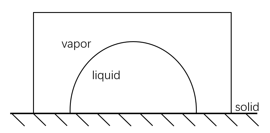
Figure 2: Schematic diagram of a liquid-vapor-solid system

By using the Young’s equation, (53) can be further simplified to

$$\tilde{\mathcal{E}}=\gamma_{LV}|\Gamma_{LV}|+\gamma_{SL}|\Gamma_{SL}|+\gamma_{SV}|\Gamma_{SV}|=\gamma_{LV}|\Gamma_{LV}|-\gamma_{LV}\cos\theta_{Y}|\Gamma_{SL}|+C,$$ (55)

where $C=\gamma_{SV}|\Gamma_{S}|$.

Consider a general two dimensional non-closed curve $\tilde{\Gamma}(t)$, where the left and right endpoints lie on the same horizontal line, as shown in Figure 3. Let $\vec{x}(s,t)$ denote the points on the curve $\tilde{\Gamma}(t)$, where $s$ is the arc length parameter. We define the counterclockwise direction as the positive direction of the curve $\tilde{\Gamma}(t)$, and denote its length as $L(t)$. The right endpoint is represented by $\vec{x}(0,t)$ and the left endpoint by $\vec{x}(L,t)$. The left and right contact angles between the curve $\tilde{\Gamma}(t)$ and the horizontal line are denoted by $\theta_{L}$ and $\theta_{0}$, respectively. The unit tangent vector is denoted by $\vec{\tau}$ and the outward unit normal vector by $\vec{n}$. Under the constraint that the area enclosed by $\tilde{\Gamma}(t)$ and the horizontal line remains constant, we aim to derive the evolution equation of the non-closed curve $\tilde{\Gamma}(t)$ under mean curvature flow.

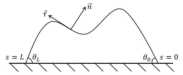
Figure 3: A non-closed curve whose two endpoints always lie on the same horizontal line

The total surface energy in (55) can be rewritten as

$$\tilde{\mathcal{E}}=\gamma[L(t)-|\vec{x}(0,t)-\vec{x}(L,t)|\cos\theta_{Y}]+C,$$ (56)

where $\gamma=\gamma_{LV}$ represents the surface energy density and $\theta_{Y}$ denotes the Young’s angle. Since the left and right endpoints of $\tilde{\Gamma}(t)$ lie on the bottom line, they possess solely horizontal velocities. Taking the horizontal right direction as the positive direction, the velocities at the left and right endpoints are denoted by $v(L)$ and $v(0)$, respectively. The changing rate of the length $L(t)$ of $\tilde{\Gamma}(t)$ with respect to time is given by (c.f. Lemma 5.1 in [lu2021efficient])

$$\frac{\text{d}L(t)}{\text{d}t}=\int_{\tilde{\Gamma}(t)}\kappa v_{n}\text{d}s+v(0)\cos\theta_{0}-v(L)\cos\theta_{L}.$$ (57)

Therefore, the changing rate of the total energy is calculated as

$$\dot{\tilde{\mathcal{E}}} =\gamma[\frac{\text{d}L(t)}{\text{d}t}-\frac{\text{d}}{\text{d}t}|\vec{x}(0,t)-\vec{x}(L,t)|\cos\theta_{Y}]$$ (58)

$$=\gamma[\int_{\tilde{\Gamma}(t)}\kappa v_{n}\text{d}s+v(0)\cos\theta_{0}-v(L)\cos\theta_{L}-\cos\theta_{Y}(v(0)-v(L))]$$

$$=\gamma[\int_{\tilde{\Gamma}(t)}\kappa v_{n}\text{d}s+v(0)(\cos\theta_{0}-\cos\theta_{Y})-v(L)(\cos\theta_{L}-\cos\theta_{Y})].$$

We suppose that the dissipation function of $\tilde{\Gamma}(t)$ is given by

$$\tilde{\Phi}=\frac{\xi_{0}}{2}\int_{\tilde{\Gamma}(t)}v_{n}^{2}\text{d}s+\frac{\xi_{1}}{2}v(0)^{2}+\frac{\xi_{1}}{2}v(L)^{2},$$ (59)

where $\xi_{0},\xi_{1}$ are positive friction coefficients. Notice we introduce additional terms $\frac{\xi_{1}}{2}v(0)^{2}$ and $\frac{\xi_{1}}{2}v(L)^{2}$ to the dissipation function $\tilde{\Phi}$, which are dissipations due to the contact line frictions. As a result, it characterize the relaxation process of the contact angles from their initial values $\theta_{L}$ and $\theta_{0}$ to the equilibrium Young’s angle $\theta_{Y}$. Then the corresponding Rayleighian is given by

$$\tilde{\mathcal{R}}=\tilde{\Phi}+\dot{\tilde{\mathcal{E}}}.$$ (60)

In wetting problems, the volume of a liquid is preserved. The time derivative of the area $\tilde{S}$ enclosed by the curve $\tilde{\Gamma}(t)$ and the bottom line is given by (c.f. Lemma5.1 in [lu2021efficient])

$$\frac{\text{d}\tilde{S}}{\text{d}t}=\int_{\tilde{\Gamma}(t)}v_{n}\text{d}s.$$ (61)

By using the Onsager principle, we minimize the Rayleighian $\tilde{\mathcal{R}}$ with respect to $v_{n},v(0),v(L)$ under the area conservation condition, i.e.

$$\min_{v_{n},v(0),v(L)}\ \tilde{\mathcal{R}},$$ (62)

$$s.t.\ \frac{\text{d}\tilde{S}}{\text{d}t}=0.$$

Introduce a Lagrangian multiplier $\lambda$, the corresponding augmented Lagrangian is defined as

$$\tilde{\mathcal{L}}(v_{n},v(0),v(L),\lambda)=\tilde{\mathcal{R}}+\lambda\frac{\text{d}\tilde{S}}{\text{d}t} =\int_{\tilde{\Gamma}(t)}(\frac{\xi_{0}}{2}v_{n}^{2}+\gamma\kappa v_{n}+\lambda v_{n})\text{d}s+\frac{\xi_{1}}{2}v(0)^{2}+\frac{\xi_{1}}{2}v(L)^{2}$$ (63)

$$\quad+\gamma[v(0)(\cos\theta_{0}-\cos\theta_{Y})-v(L)(\cos\theta_{L}-\cos\theta_{Y})].$$

We let

$$\left\{\begin{array}[]{rcl}\frac{\partial\tilde{\mathcal{L}}}{\partial v_{n}}=0\\ \frac{\partial\tilde{\mathcal{L}}}{\partial v(0)}=0\\ \frac{\partial\tilde{\mathcal{L}}}{\partial v(L)}=0\\ \frac{\partial\tilde{\mathcal{L}}}{\partial\lambda}=0.\end{array}\right.$$ (64)

This leads to the following Euler-Lagrange equation

$$\left\{\begin{array}[]{rcl}&\xi_{0}v_{n}=-(\gamma\kappa+\lambda)\\ &\xi_{1}v(0)=-\gamma(\cos\theta_{0}-\cos\theta_{Y})\\ &\xi_{1}v(L)=\gamma(\cos\theta_{L}-\cos\theta_{Y})\\ &\int_{\tilde{\Gamma}(t)}v_{n}\text{d}s=0.\end{array}\right.$$ (65)

Substitute the first equation of (65) into the last one. We get

$$\int_{\tilde{\Gamma}(t)}-(\gamma\kappa+\lambda)\text{d}s=0.$$ (66)

This implies that

$$\lambda L(t)=-\gamma\int_{\tilde{\Gamma}(t)}\kappa\text{d}s.$$ (67)

For the closed curve consisting of $\tilde{\Gamma}(t)$ and the bottom line, applying the Gauss-Bonnet formula yields

$$\int_{\tilde{\Gamma}(t)}\kappa\text{d}s+0\cdot|\vec{x}(0,t)-\vec{x}(L,t)|+\pi-\theta_{0}+\pi-\theta_{L}=2\pi.$$ (68)

This leads to

$$\int_{\tilde{\Gamma}(t)}\kappa\text{d}s=\theta_{0}+\theta_{L}.$$ (69)

Substituting the equation (69) into (67), we have

$$\lambda=-\frac{\gamma(\theta_{0}+\theta_{L})}{L(t)}.$$ (70)

Thus, we obtain the normal velocity of the curve $\tilde{\Gamma}(t)$

$$\xi_{0}v_{n}=-\gamma(\kappa-\frac{\theta_{0}+\theta_{L}}{L(t)}).$$ (71)

Substituting the equation (65) and the equation (71) into (58), we get

$$\dot{\tilde{\mathcal{E}}} =\gamma[\int_{\tilde{\Gamma}(t)}\kappa v_{n}\text{d}s+v(0)(\cos\theta_{0}-\cos\theta_{Y})-v(L)(\cos\theta_{L}-\cos\theta_{Y})]$$ (72)

$$=\gamma[\int_{\tilde{\Gamma}(t)}-\xi_{0}^{-1}\gamma\kappa(\kappa-\frac{\theta_{0}+\theta_{L}}{L(t)})\text{d}s-\xi_{1}^{-1}\gamma(\cos\theta_{0}-\cos\theta_{Y})^{2}-\xi_{1}^{-1}\gamma(\cos\theta_{L}-\cos\theta_{Y})^{2}]$$

$$=-\gamma^{2}[\int_{\tilde{\Gamma}(t)}\xi_{0}^{-1}(\kappa^{2}-\kappa\frac{\theta_{0}+\theta_{L}}{L(t)})\text{d}s+\xi_{1}^{-1}(\cos\theta_{0}-\cos\theta_{Y})^{2}+\xi_{1}^{-1}(\cos\theta_{L}-\cos\theta_{Y})^{2}].$$

By (69), we can easily derive

$$\int_{\tilde{\Gamma}(t)}\kappa(\kappa-\frac{\theta_{0}+\theta_{L}}{L(t)})\text{d}s=\int_{\tilde{\Gamma}(t)}(\kappa-\frac{\theta_{0}+\theta_{L}}{L(t)})^{2}\text{d}s.$$

This directly leads to

$$\dot{\tilde{\mathcal{E}}}=-2\tilde{\Phi}_{h}\leq 0.$$ (73)

This implies that the total energy decreases with respect to time for the system characterized by the dynamic equation (65).

Similarly to the problems in the previous two section, we ignore the tangential velocity, the dynamic equation for a wetting problem can be described by

$$\left\{\begin{array}[]{rcl}&\vec{v}=-\xi_{0}^{-1}\gamma(\kappa-\frac{\theta_{0}+\theta_{L}}{|\tilde{\Gamma}(t)|})\vec{n}\\ &v(0)=-\xi_{1}^{-1}\gamma(\cos\theta_{0}-\cos\theta_{Y})\\ &v(L)=\xi_{1}^{-1}\gamma(\cos\theta_{L}-\cos\theta_{Y}),\end{array}\right.$$ (74)

where $\vec{v}$ denotes the velocity of the curve, $v(0)$ and $v(L)$ are respectively the horizontal velocity of the two endpoints, $\theta_{L}$ and $\theta_{0}$ denote the left and right contact angles of the curve with the bottom line, and $|\tilde{\Gamma}(t)|$ denotes the length of the curve.

5.2 Discretization of the dynamic equation by the Onsager principle

In this section, we aim to numercially solve the dynamic equation (65). Suppose that the curve $\tilde{\Gamma}(t)$ can be approximated by piecewise linear segments, as illustrated in Figure 4. Denote the nodes by

$$\vec{x}_{1}(t),\vec{x}_{2}(t),...,\vec{x}_{n}(t).$$ (75)

Where $\vec{x}_{i}(t)=(x_{i}^{(1)}(t),x_{i}^{(2)}(t))^{T}\ (1\leq i\leq n)$, the right endpoint $\vec{x}_{1}(t)=(x_{1}^{(1)}(t),0)^{T}$ and the left endpoint $\vec{x}_{n}(t)=(x_{n}^{(1)}(t),0)^{T}$. The line segments connecting adjacent nodes are denoted by $\tilde{\Gamma}_{i}(t)=\overline{\vec{x}_{i}(t)\vec{x}_{i+1}(t)}\ (1\leq i\leq n-1)$. Consequently, the approximate curve is given by $\tilde{\Gamma}_{h}(t)=\bigcup\limits_{i=1}^{n-1}\tilde{\Gamma}_{i}(t)$.

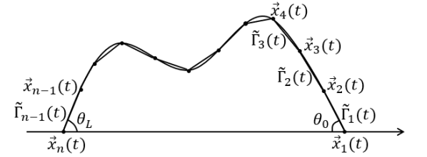
Figure 4: Selection of interpolation points

We will derive the dynamic equation for $\tilde{\Gamma}_{h}(t)$ by using the Onsager principle. Similar to that in Section 3.2, for a line segment $\tilde{\Gamma}_{i}(t)(1\leq i\leq n-1)$, the points on the segment can be expressed as $\vec{x}_{h}(t)=\mu[\vec{x}_{i+1}(t)-\vec{x}_{i}(t)]+\vec{x}_{i}(t)=(1-\mu)\vec{x}_{i}(t)+\mu\vec{x}_{i+1}(t),$ where $0\leq\mu=\frac{s}{|\vec{x}_{i+1}-\vec{x}_{i}|}\leq 1$ is a parameter. The velocity of each point $\vec{x}_{h}(t)$ is given by $\vec{v}_{h}(t)=(1-\mu)\dot{\vec{x}}_{i}(t)+\mu\dot{\vec{x}}_{i+1}(t).$ The unit tangent vector of $\tilde{\Gamma}_{i}(t)$ is calculated by $\vec{\tau}_{i}=\frac{\vec{x}_{i+1}(t)-\vec{x}_{i}(t)}{|\vec{x}_{i+1}(t)-\vec{x}_{i}(t)|}.$ The outward unit normal vector is given by $\vec{n}_{i}=\frac{P[\vec{x}_{i+1}(t)-\vec{x}_{i}(t)]}{|\vec{x}_{i+1}(t)-\vec{x}_{i}(t)|}.$

For the discrete curve $\tilde{\Gamma}_{h}(t)$, the discrete energy is calculated by

$$\tilde{\mathcal{E}}_{h} =\gamma[|\tilde{\Gamma}_{h}(t)|-|\vec{x}_{1}(t)-\vec{x}_{n}(t)|\cos\theta_{Y}]+C$$ (76)

$$=\gamma\{\sum_{i=1}^{n-1}|\vec{x}_{i+1}(t)-\vec{x}_{i}(t)|-[x_{1}^{(1)}(t)-x_{n}^{(1)}(t)]\cos\theta_{Y}\}+C.$$

The discrete dissipation funtion is calculated by

$$\tilde{\Phi}_{h} =\frac{1}{2}\int_{\tilde{\Gamma}_{h}(t)}v_{h,n}^{2}\text{d}s+\frac{1}{2}v_{h}(0)^{2}+\frac{1}{2}v_{h}(L)^{2}$$ (77)

$$=\frac{1}{2}\sum_{i=1}^{n-1}\int_{\tilde{\Gamma}_{i}(t)}[\vec{v}_{h}(t)\cdot\vec{n}_{i}]^{2}\text{d}s+\frac{1}{2}[\dot{x}_{1}^{(1)}(t)]^{2}+\frac{1}{2}[\dot{x}_{n}^{(1)}(t)]^{2}.$$

Taking the horizontal right direction as the positive direction, here we denote the normal velocity at the two endpoints by

$$v_{h,n}(0)=v_{h}(0)\sin\theta_{0}=\dot{x}_{1}^{(1)}(t)\sin\theta_{0},\quad v_{h,n}(L)=-v_{h}(L)\sin\theta_{L}=-\dot{x}_{n}^{(1)}(t)\sin\theta_{L},$$ (78)

where

$$\sin\theta_{0}=\frac{x_{2}^{(2)}(t)}{|\vec{x}_{2}(t)-\vec{x}_{1}(t)|},\quad\sin\theta_{L}=\frac{x_{n-1}^{(2)}(t)}{|\vec{x}_{n}(t)-\vec{x}_{n-1}(t)|}.$$ (79)

Denote by $\tilde{S}_{h}$ the area enclosed by the discrete curve $\tilde{\Gamma}_{h}(t)$ and the bottom line. Then the changing rate of $\tilde{S}_{h}$ with respect to time is calculated as

$$\frac{\text{d}\tilde{S}_{h}}{\text{d}t} =\int_{\tilde{\Gamma}_{h}(t)}v_{h,n}\text{d}s=\sum_{i=1}^{n-1}\int_{\tilde{\Gamma}_{i}(t)}\vec{v}_{h}(t)\cdot\vec{n}_{i}\text{d}s$$ (80)

By using the Onsager principle, we minimize the discrete Rayleighian with respect to $\dot{\vec{x}}_{i}$ under the area conservation constraint, i.e.

$$\min_{\dot{\vec{x}}_{i}}\ \tilde{\mathcal{R}}_{h}:=\tilde{\Phi}_{h}+\dot{\tilde{\mathcal{E}}}_{h},$$ (81)

$$s.t.\ \frac{\text{d}\tilde{S}_{h}}{\text{d}t}=0.$$

The corresponding discrete augmented Lagrangian is defined as

$$\tilde{\mathcal{L}}_{h}(\dot{\vec{x}}_{i},\lambda)=\tilde{\mathcal{R}}_{h}+\lambda\frac{\text{d}\tilde{S}_{h}}{\text{d}t}.$$ (82)

We set

$$\left\{\begin{array}[]{rcl}\frac{\partial\tilde{\mathcal{L}}_{h}}{\partial\dot{\vec{x}}_{i}}=0\\ \frac{\partial\tilde{\mathcal{L}}_{h}}{\partial\lambda}=0.\end{array}\right.$$ (83)

The corresponding Euler-Lagrange equation is given by

$$\left\{\begin{array}[]{ll}\frac{\partial\tilde{\Phi}_{h}}{\partial\dot{x}_{1}^{(1)}}+\lambda\frac{\partial(\tilde{S}_{h})_{t}}{\partial\dot{x}_{1}^{(1)}}=-\frac{\partial\tilde{\mathcal{E}}_{h}}{\partial x_{1}^{(1)}}\quad for\quad i=1\\ \frac{\partial\tilde{\Phi}_{h}}{\partial\dot{\vec{x}}_{i}}+\lambda\frac{\partial(\tilde{S}_{h})_{t}}{\partial\dot{\vec{x}}_{i}}=-\frac{\partial\tilde{\mathcal{E}}_{h}}{\partial\vec{x}_{i}}\qquad\!for\quad 2\leq i\leq n-1\\ \frac{\partial\tilde{\Phi}_{h}}{\partial\dot{x}_{n}^{(1)}}+\lambda\frac{\partial(\tilde{S}_{h})_{t}}{\partial\dot{x}_{n}^{(1)}}=-\frac{\partial\tilde{\mathcal{E}}_{h}}{\partial x_{n}^{(1)}}\quad for\quad i=n\\ \frac{\text{d}\tilde{S}_{h}}{\text{d}t}=0.\end{array}\right.$$ (84)

This is a system of differential-algebraic equations with respect to $\dot{x}_{1}^{(1)},\dot{\vec{x}}_{i}\ (2\leq i\leq n-1),\dot{x}_{n}^{(1)}$ and $\lambda$.

For convenience of representation, we add two equations $\dot{x}_{1}^{(2)}=0,\dot{x}_{n}^{(2)}=0$ to (84) and denote $\dot{X}=(\dot{\vec{x}}_{1}^{T},\dot{\vec{x}}_{2}^{T},...,\dot{\vec{x}}_{n}^{T},\lambda)^{T}$. Observe that $\tilde{\Phi}_{h}$ is a quadratic function with respect to $\dot{\vec{x}}_{i}\ (1\leq i\leq n)$. Then the system (84) can be rewritten as

$$\tilde{A}\dot{X}=\tilde{G},$$ (85)

where the coefficient matrix $\tilde{A}$ is symmetric and the right-hand term $\tilde{G}=(\tilde{\vec{g}}_{1}^{T},\tilde{\vec{g}}_{2}^{T},...,\tilde{\vec{g}}_{n}^{T},\tilde{g}_{n+1})^{T}$. The explicit formulas for $\tilde{A}$ and $\tilde{G}$ are given in Appendix.

We can easily prove the discrete energy dissipative property of the ODE system (85).

Theorem 5.1.

Suppose $\dot{X}=(\dot{\vec{x}}_{1}^{T},\dot{\vec{x}}_{2}^{T},...,\dot{\vec{x}}_{n}^{T},\lambda)^{T}$ is the solution of the equation set (85), then we have

$$\frac{\text{d}\tilde{\mathcal{E}}_{h}}{\text{d}t}=-2\tilde{\Phi}_{h}\leq 0,$$ (86)

where the equality holds if and only if $\dot{\vec{x}}_{i}=0\ (0\leq i\leq n)$.

The proof is similar to that of Theorem 4.1 and we skip it for simplicity in presentation.

As in the section 3.3, we add a penalty term to the energy function $\tilde{\mathcal{E}}_{h}$ in order to make the nodes on the discrete curve uniformly distributed. The modified energy function is denoted by

$$\tilde{\mathcal{E}}_{h}^{\delta}=\tilde{\mathcal{E}}_{h}+\delta\sum_{i=1}^{n-2}\bigl{(}\frac{|\tilde{\Gamma}_{i}(t)|}{|\tilde{\Gamma}_{i+1}(t)|}-1\bigr{)}^{2}.$$ (87)

We generally take $\delta=\frac{1}{n-2}$ in order to reduce the impact of the penalty term on $\tilde{\mathcal{E}}_{h}$. The corresponding Euler-Lagrange equation is

$$\tilde{A}\dot{X}=\tilde{G}^{\delta}.$$ (88)

6 Numerical experiments

We will present some experimental simulation results in this section. In simulations, we solve this problems using the improved Euler’s method as follows

$$\left\{\begin{array}[]{rcl}\text{predictor}:{\tilde{X}}^{k+1}&=&X^{k}+\dot{X}^{k}\Delta t\\ \text{corrector}:X^{k+1}&=&X^{k}+\frac{(\dot{X}^{k}+\dot{{\tilde{X}}}^{k+1})}{2}\Delta t.\end{array}\right.$$ (89)

where $X^{k}$ represents the position of the curve at time $t_{k}$. For the equation (26), $\dot{X}^{k}=A^{-1}(X^{k})G^{\delta}(X^{k})$ denotes the time derivative of $X^{k}$, and $\dot{\tilde{X}}^{k+1}=A^{-1}(\tilde{X}^{k+1})G^{\delta}(\tilde{X}^{k+1})$. For the equations (50) and (85), we use $\hat{A}$, $\hat{G}$ and $\tilde{A}$, $\tilde{G}$ respectively.

6.1 Mean curvature flow

6.1.1 The evolution of a circular curve

We consider the evolution of a circle under mean curvature flow. Notice that the curve will always be circular in this case. We can assume that

$$\Gamma(t):=\{\vec{x}(t,\alpha)=\rho(t)(\cos\alpha,\sin\alpha)^{T},\quad 0\leq\alpha\leq 2\pi\},$$ (90)

where $\rho(t)$ denotes the radius of the circle at time $t$, and it satisfies the initial condition $\rho(0)=R_{0}$. By substituting the equation (90) into Equation (16), we have

$$\frac{\text{d}\rho}{\text{d}t}=-\frac{1}{\rho(t)}.$$ (91)

Solving the equation (91), we can obtain the evolution equation of the curve $\Gamma(t)$:

$$\vec{x}(t,\alpha)=\sqrt{R_{0}^{2}-2t}(\cos\alpha,\sin\alpha)^{T},\quad 0\leq\alpha\leq 2\pi.$$ (92)

Hence, under mean curvature flow, a circle of initial radius $R_{0}$ gradually shrinks to a circle of radius $\sqrt{R_{0}^{2}-2t}$ at time $t$, and eventually collapses to a point at time $t=\frac{R_{0}^{2}}{2}$.

In our numerical simulations, the initial curve is taken as the unit circle. The circle is discretized uniformly with $\vec{x}_{i}=(\cos\frac{2\pi}{n}i,\sin\frac{2\pi}{n}i)^{T}$. The shape of the curve at some time steps are shown in Figure 5, while the change of the discrete energy function $\mathcal{E}_{h}(t)$ over time is shown in Figure 6. We can see that discrete curves are circular and the discrete energy decreases gradually.

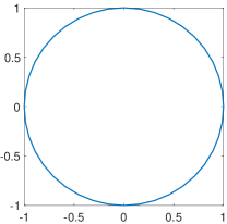
(a) t=0

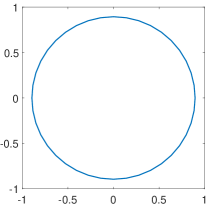
(b) t=0.1

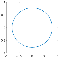
(c) t=0.2

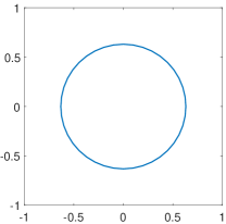
(d) t=0.3

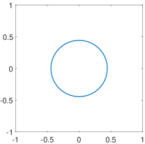
(e) t=0.4

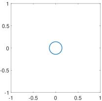
(f) t=0.488

Figure 5: Evolution of a unit circle under mean curvature flow (n=40).

Figure 6: The change of the discrete energy $\mathcal{E}_{h}(t)$ with respect to time.

Since the explicit solution is known in this example (as shown in (92)), we can compute the errors of the numerical slutions. We denote the point on the discrete curve $\Gamma_{h}(t)$ by $\vec{x}_{h}(t,\alpha)$. We define the error as

$$err:=\text{dist}(\vec{x}_{h}(t),\Gamma(t)).$$ (93)

The convergence order, which characterizes the rate of convergence, is calculated as follows

$$order:=\frac{\ln(\frac{err_{k}}{err_{k+1}})}{\ln(\frac{n_{k+1}}{n_{k}})}.$$ (94)

We set $T=0.2$ and choose a time step size of $\Delta t=0.00025$, which is small enough so that the error with respect to time discretization is of higher order. Taking the number of nodes as $n=5,10,20,40,80$, the corresponding numerical errors and convergence order are presented in Table 1. We could see the method has second order convergent in distance norm with respect to the spacial mesh size.

Table 1: Error and convergence order of the numerical method in Section 3.2.

n	5	10	20	40	80
err	0.0816	0.0178	0.0043	0.0011	2.6563e-04
order	-	2.1967	2.0495	1.9668	2.0500

6.1.2 The evolution of a flower-shaped curve

We consider the evolution of a flower-shaped curve under mean curvature flow. The parametric equation for the initial flower-shaped curve is given by:

$$\vec{x}(\alpha)=((2-2^{\sin(5\alpha)})\cos\alpha,(2-2^{\sin(5\alpha)})\sin\alpha)^{T},\quad 0\leq\alpha\leq 2\pi.$$ (95)

We discretize the curve uniformly in $\alpha$ by setting $\vec{x}_{i}=\vec{x}(\alpha_{i})$ with $\alpha_{i}=\frac{2\pi}{n}i$. The evolution of the curve is plotted in Figure 7, and the change of the discrete energy function $\mathcal{E}_{h}(t)$ is illustrated in Figure 8. We can see that the curve gradually changes to a circular shape and also shrinks in length. We can also see how the discrete energy function gradually decreases as the curve evolves under mean curvature flow.

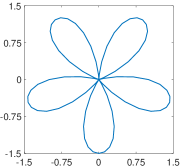
(a) t=0

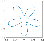
(b) t=0.03

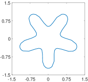
(c) t=0.06

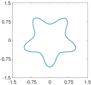
(d) t=0.09

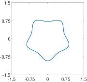
(e) t=0.12

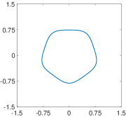
(f) t=0.15

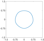
(g) t=0.18

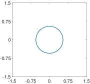
(h) t=0.3

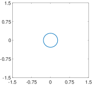
(i) t=0.41

Figure 7: Evolution of a flower-shaped curve under mean curvature flow (n=80).

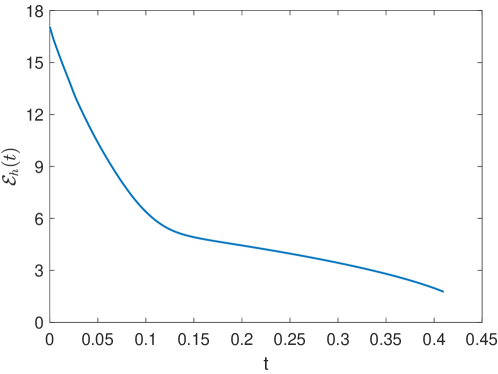
Figure 8: The change of the discrete energy $\mathcal{E}_{h}(t)$ with respect to time.

6.2 Volume preserving mean curvature flow

In this subsection, we show numerical simulations for the volume preserving mean curvature flows. We choose the same initial curve as that in Section 6.1.2. We discretize the curve (95) uniformly in $\alpha$ by setting $\vec{x}_{i}=\vec{x}(\alpha_{i})$ with $\alpha_{i}=\frac{2\pi}{n}i$. The evolution of the curve is plotted in Figure 9. We can see that the flower-shaped curve slowly becomes convex and eventually evolves into a circular shape. Due to the constraint that the enclosed area remains constant, the shape of the curve will not change after it becomes a circle, i.e., it will reach a stationary state. The discrete energy function $\mathcal{E}_{h}(t)$ changes with time as shown in Figure 10. We can see that the discrete energy function decreases in early stage and then approaches to a constant when the system goes to the stationary state.

(a) t=0

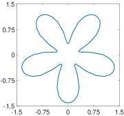
(b) t=0.03

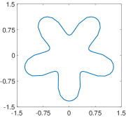
(c) t=0.06

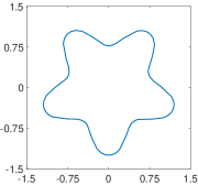
(d) t=0.09

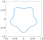
(e) t=0.12

(f) t=0.15

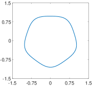
(g) t=0.18

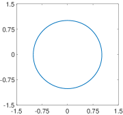
(h) t=0.3

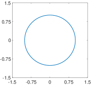
(i) t=0.4

Figure 9: Evolution of a flower-shaped curve under the volume preserving mean curvature flow (n=80).

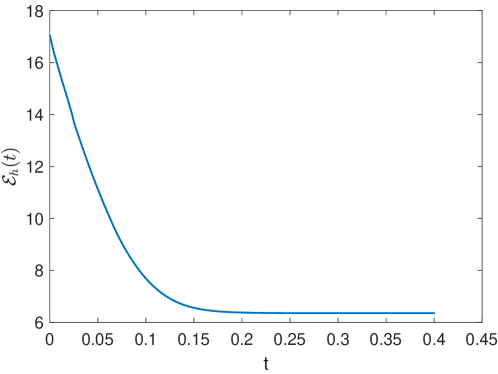
Figure 10: The change of the discrete energy $\mathcal{E}_{h}(t)$ with respect to time.

6.3 Wetting problems

We consider the $x$-axis as the horizontal line with the positive direction to the right. The initial curve is taken as a unit semicircle

$$\tilde{\Gamma}(0):\vec{x}(\alpha)=(\cos\alpha,\sin\alpha)^{T}\quad(0\leq\alpha\leq\pi).$$ (96)

Under the constraint that the area enclosed by $\tilde{\Gamma}(t)$ and the $x$-axis remains constant, when $\tilde{\Gamma}(t)$ reaches a stationary state under mean curvature flow, the energy no longer changes, i.e., the changing rate of the energy over time $\dot{\tilde{\mathcal{E}}}=0$. From the expression (58) of $\dot{\tilde{\mathcal{E}}}$, the left and right contact angles of the curve at stationary state are equal to the Young’s angle.

We discretize the curve uniformly in $\alpha$ by setting $\vec{x}_{i}=\vec{x}(\alpha_{i})$ with $\alpha_{i}=\frac{\pi}{n}i$ and take the Young’s angle $\theta_{Y}$ as $\frac{2\pi}{3}$ and $\frac{\pi}{3}$ respectively. The evolution of the curve is plotted in Figure 11 while the change of the discrete energy function $\tilde{\mathcal{E}}_{h}$ over time is shown in Figure 12. We can see that the droplet gradually change its shape from a semi-circle to a circular shape with stationary contact angles. From Figure 12 we can see that the discrete energy function initially decreases to a constant value.

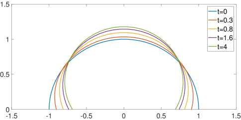
(a) $\theta_{Y}=\frac{2\pi}{3}$

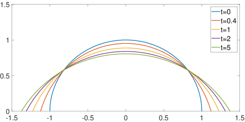
(b) $\theta_{Y}=\frac{\pi}{3}$

Figure 11: Evolution of unit semicircles in the wetting problem (n=40).

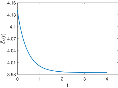
(a) $\theta_{Y}=\frac{2\pi}{3}$

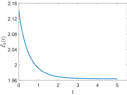
(b) $\theta_{Y}=\frac{\pi}{3}$

Figure 12: The change of the discrete energy $\tilde{\mathcal{E}}_{h}(t)$ with respect to time.

The exact solutions of wetting problem can be affected by lateral displacement of the curve. We thus define the error as the difference of the stationary-state energy between the discrete curve and the smooth curve, i.e.

$$err:=|\tilde{\mathcal{E}}-\tilde{\mathcal{E}}_{h}|.$$ (97)

The convergence order is calculated as in Equation (94). We conducted numerical simulations with different parameters to assess the accuracy and convergence of the method. For the case where Young’s angle is $\theta_{Y}=\frac{2\pi}{3}$, we use a time step size of $\Delta t=10^{-5}$ and varied the number of nodes as $n=5,10,20,40,80$. The simulation was performed for $T=4$ time steps. The resulting errors and convergence order are summarized in Table 2. Similarly, for the case where Young’s angle is $\theta_{Y}=\frac{\pi}{3}$, we used the same time step size and varied the number of nodes as before. The simulation was performed for $T=5$ time steps, and the corresponding errors and convergence order are presented in Table 3. We could see the method has second order convergent with respect to the spacial mesh size.

Table 2: $\theta_{Y}=\frac{2\pi}{3}$, error and convergence order of the numerical method in Section 5.2.

n	5	10	20	40	80
err	0.0553	0.0107	0.0023	5.0217e-04	9.3273e-05
order	-	2.3731	2.2035	2.2075	2.4286

Table 3: $\theta_{Y}=\frac{\pi}{3}$, error and convergence order of the numerical method in Section 5.2.

n	5	10	20	40	80
err	0.0624	0.0122	0.0025	4.9335e-04	5.9605e-05
order	-	2.3525	2.2802	2.3494	3.0491

7 Conclusions

In this paper, we develop a novel finite element method for mean curvature flows by using the Onsager principle as an approximation tool. The key feature of the method is that the discrete scheme preserves the energy dissipation relations of the Onsager principle. This is important for many applications. We apply the method to three different problems, namely the simple mean curvature flow, the volume preserving mean curvature flow and a wetting problem on substrate. Numerical examples show that the method works well for all the three problems.

There are several problems we need to study in the future. Firstly, we apply an explicit Euler scheme for the time discretization. The scheme is stable only the time step is small enough. We need consider implicit or semi-implicit scheme to improve the stability of the scheme. Another important issue is on the quality of meshes of the discrete geometric flow. To avoid mesh degeneracy and entanglement, we add a penalty term to the energy. The technique works well only when we need choose the penalty parameter and the time step properly. It is known that some other methods have properties to keep the mesh equally distributed in arc length. It is interesting to combine these techniques with our method. In addition, it is interesting to do numerical analysis of the method and also extend the method ot higher order approximations and other geometric flows.

8 Acknowledgement

The work was partially supported by NSFC 11971469 and 12371415. We also thank Professor Wei Jiang for help discussions.

Appendix

In sections 3-5, we derived multiple systems of equations. For convenience of the reader, we will show the specific form of Equations (26) (32) (50) and (85) below.

Firstly, for Equation (26), the coefficient matrix $A$ and the right-hand term $G$ are computed as follows:

$$\begin{gathered}A=\begin{pmatrix}A_{11}&A_{12}&&&A_{1n}\\ A_{21}&A_{22}&A_{23}\\ \quad&\ddots&\ddots&\ddots\\ &&A_{n-1,n-2}&A_{n-1,n-1}&A_{n-1,n}\\ A_{n,1}&&&A_{n,n-1}&A_{n,n}\end{pmatrix}.\end{gathered}$$

where the elements $A_{ij}(1\leq i,j\leq n)$ are square matrixes of order 2. Denote by $I_{2}$ the unit matrix of order 2. Then we have

$$A_{ii}=\frac{|\vec{x}_{i}(t)-\vec{x}_{i-1}(t)|+|\vec{x}_{i+1}(t)-\vec{x}_{i}(t)|}{3}I_{2},\quad i=1,...n-1,$$ (98)

$$A_{i,i+1}=A_{i+1,i}=\frac{|\vec{x}_{i+1}(t)-\vec{x}_{i}(t)|}{6}I_{2},\quad i=1,...n-1;$$

and

$$A_{nn}=\frac{|\vec{x}_{n}(t)-\vec{x}_{n-1}(t)|+|\vec{x}_{1}(t)-\vec{x}_{n}(t)|}{3}I_{2},$$ (99)

$$A_{n,1}=A_{1,n}=\frac{|\vec{x}_{1}(t)-\vec{x}_{n}(t)|}{6}I_{2}.$$

The right-hand term $G=(\vec{g}_{1}^{T},\vec{g}_{2}^{T},...,\vec{g}_{n}^{T})^{T}$ with

$$\vec{g}_{i}=-\frac{\partial\mathcal{E}_{h}}{\partial\vec{x}_{i}}=\frac{\vec{x}_{i+1}(t)-\vec{x}_{i}(t)}{|\vec{x}_{i+1}(t)-\vec{x}_{i}(t)|}-\frac{\vec{x}_{i}(t)-\vec{x}_{i-1}(t)}{|\vec{x}_{i}(t)-\vec{x}_{i-1}(t)|},\quad i=1,...,n-1,$$ (100)

and

$$\vec{g}_{n}=-\frac{\partial\mathcal{E}_{h}}{\partial\vec{x}_{n}}=\frac{\vec{x}_{1}(t)-\vec{x}_{n}(t)}{|\vec{x}_{1}(t)-\vec{x}_{n}(t)|}-\frac{\vec{x}_{n}(t)-\vec{x}_{n-1}(t)}{|\vec{x}_{n}(t)-\vec{x}_{n-1}(t)|}.$$ (101)

Secondly, for Equation (32), the right-hand term $G^{\delta}=((\vec{g}_{1}^{\delta})^{T},(\vec{g}_{2}^{\delta})^{T},...,(\vec{g}_{n}^{\delta})^{T})^{T}$ is computed as follows:

$$g_{i}^{\delta}=-\frac{\partial\mathcal{E}_{h}^{\delta}}{\partial\vec{x}_{i}} =\frac{\vec{x}_{i+1}-\vec{x}_{i}}{|\vec{x}_{i+1}-\vec{x}_{i}|}-\frac{\vec{x}_{i}-\vec{x}_{i-1}}{|\vec{x}_{i}-\vec{x}_{i-1}|}$$ (102)

$$\ +2\delta(\frac{|\vec{x}_{i+1}-\vec{x}_{i}|}{|\vec{x}_{i+2}-\vec{x}_{i+1}|}-1)\frac{\vec{x}_{i+1}-\vec{x}_{i}}{|\vec{x}_{i+2}-\vec{x}_{i+1}|\cdot|\vec{x}_{i+1}-\vec{x}_{i}|}$$

$$\ -2\delta(\frac{|\vec{x}_{i}-\vec{x}_{i-1}|}{|\vec{x}_{i+1}-\vec{x}_{i}|}-1)\frac{\frac{\vec{x}_{i}-\vec{x}_{i-1}}{|\vec{x}_{i}-\vec{x}_{i-1}|}|\vec{x}_{i+1}-\vec{x}_{i}|+|\vec{x}_{i}-\vec{x}_{i-1}|\frac{\vec{x}_{i+1}-\vec{x}_{i}}{|\vec{x}_{i+1}-\vec{x}_{i}|}}{|\vec{x}_{i+1}-\vec{x}_{i}|^{2}}$$

$$\ +2\delta(\frac{|\vec{x}_{i-1}-\vec{x}_{i-2}|}{|\vec{x}_{i}-\vec{x}_{i-1}|}-1)\frac{|\vec{x}_{i-1}-\vec{x}_{i-2}|(\vec{x}_{i}-\vec{x}_{i-1})}{|\vec{x}_{i}-\vec{x}_{i-1}|^{3}}.$$

Next, for Equation (50), the coefficient matrix $\hat{A}$ and the right-hand term $\hat{G}$ are computed as follows:

$$\begin{gathered}\hat{A}=\begin{pmatrix}A_{11}&A_{12}&&&&&&A_{1n}&\vec{b}_{1,n+1}\\ A_{21}&A_{22}&A_{23}\\ \quad&\ddots&\ddots&\ddots&&&&&\vdots\\ &&A_{i,i-1}&A_{i,i}&A_{i,i+1}\\ &&&A_{i+1,i}&A_{i+1,i+1}&A_{i+1,i+2}\\ &&&&\ddots&\ddots&\ddots&&\vdots\\ &&&&&A_{n-1,n-2}&A_{n-1,n-1}&A_{n-1,n}&\vec{b}_{n-1,n+1}\\ A_{n,1}&&&&&&A_{n,n-1}&A_{n,n}&\vec{b}_{n,n+1}\\ \vec{b}_{1,n+1}^{T}&&\ldots&&&\ldots&\vec{b}_{n-1,n+1}^{T}&\vec{b}_{n,n+1}^{T}&0\end{pmatrix},\end{gathered}$$

and $\hat{G}=(\vec{g}_{1}^{T},\vec{g}_{2}^{T},...,\vec{g}_{n}^{T},g_{n+1})^{T}$. Where the formulations of $A_{ij}(1\leq i,j\leq n)$ and $\vec{g}_{i}\ (1\leq i\leq n)$ are given in Equations (98), (99), (100) and (101), respectively. Inaddition, we have $g_{n+1}=0$. The elements in last row and last column of $\hat{A}$ are given by

$$\vec{b}_{1,n+1}=\frac{P}{2}[\vec{x}_{2}(t)-\vec{x}_{n}(t)],$$ (103)

$$\vec{b}_{i,n+1}=\frac{P}{2}[\vec{x}_{i+1}(t)-\vec{x}_{i-1}(t)],\quad i=2,...,n;$$

where $\vec{b}_{i,n+1}(1\leq i\leq n)$ are two dimensional column vectors.

Finally, for Equation (85), the coefficient matrix $\tilde{A}$ and the right-hand term $\tilde{G}$ are computed as follows:

$$\begin{gathered}\tilde{A}=\begin{pmatrix}\tilde{A}_{11}&\tilde{A}_{12}&&&&&&&\tilde{\vec{b}}_{1,n+1}\\ \tilde{A}_{21}&\tilde{A}_{22}&\tilde{A}_{23}\\ \quad&\ddots&\ddots&\ddots&&&&&\vdots\\ &&\tilde{A}_{i,i-1}&\tilde{A}_{i,i}&\tilde{A}_{i,i+1}\\ &&&\tilde{A}_{i+1,i}&\tilde{A}_{i+1,i+1}&\tilde{A}_{i+1,i+2}\\ &&&&\ddots&\ddots&\ddots&&\vdots\\ &&&&&\tilde{A}_{n-1,n-2}&\tilde{A}_{n-1,n-1}&\tilde{A}_{n-1,n}&\tilde{\vec{b}}_{n-1,n+1}\\ &&&&&&\tilde{A}_{n,n-1}&\tilde{A}_{n,n}&\tilde{\vec{b}}_{n,n+1}\\ \tilde{\vec{b}}^{T}_{1,n+1}&&\ldots&&&\ldots&\tilde{\vec{b}}^{T}_{n-1,n+1}&\tilde{\vec{b}}^{T}_{n,n+1}&0\end{pmatrix}.\end{gathered}$$

Where $\tilde{A}_{ij}(1\leq i,j\leq n)$ are square matrixes of order 2, and $\tilde{\vec{b}}_{i,n+1}(1\leq i\leq n)$ are two dimensional column vectors. The diagonal elements of the $2n$-order principal subblock of $\tilde{A}$ are computed as

$$\tilde{A}_{11}=\left(\begin{array}[]{cc}\frac{\xi_{0}x_{2}^{(2)}(t)\sin\theta_{0}}{3}+\xi_{1}&0\\ 0&1\end{array}\right)\quad for\quad i=1$$ (104)

$$\tilde{A}_{ii}=\xi_{0}\frac{|\vec{x}_{i}(t)-\vec{x}_{i-1}(t)|+|\vec{x}_{i+1}(t)-\vec{x}_{i}(t)|}{3}I_{2}\quad for\quad 2\leq i\leq n-1$$

$$\tilde{A}_{nn}=\left(\begin{array}[]{cc}\frac{\xi_{0}x_{n-1}^{(2)}(t)\sin\theta_{L}}{3}+\xi_{1}&0\\ 0&1\end{array}\right)\quad for\quad i=n.$$

where

$$\sin\theta_{0}=\frac{x_{2}^{(2)}(t)}{|\vec{x}_{2}(t)-\vec{x}_{1}(t)|},\quad\sin\theta_{L}=\frac{x_{n-1}^{(2)}(t)}{|\vec{x}_{n}(t)-\vec{x}_{n-1}(t)|}.$$ (105)

The minor diagonal elements of the $2n$-order principal subblock of $\tilde{A}$ are computed as

$$\tilde{A}_{21}=\tilde{A}_{12}^{T}=(\frac{\xi_{0}x_{2}^{(2)}(t)\vec{n}_{1}}{6},\vec{0})\quad for\quad i=1$$ (106)

$$\tilde{A}_{i,i+1}=\tilde{A}_{i+1,i}^{T}=\xi_{0}\frac{|\vec{x}_{i+1}(t)-\vec{x}_{i}(t)|}{6}I_{2}\quad for\quad 2\leq i\leq n-2$$

$$\tilde{A}_{n-1,n}=\tilde{A}_{n,n-1}^{T}=(-\frac{\xi_{0}x_{n-1}^{(2)}(t)\vec{n}_{n-1}}{6},\vec{0})\quad for\quad i=n-1.$$

The last row and column of $\tilde{A}$ are calculated as

$$\tilde{\vec{b}}_{1,n+1}=(\frac{x_{2}^{(2)}(t)}{2},0)^{T}\quad for\quad i=1$$ (107)

$$\tilde{\vec{b}}_{i,n+1}=\frac{P}{2}[\vec{x}_{i+1}(t)-\vec{x}_{i-1}(t)]\quad for\quad 2\leq i\leq n-1.$$

$$\tilde{\vec{b}}_{n,n+1}=(-\frac{x_{n-1}^{(2)}(t)}{2},0)^{T}\quad for\quad i=n.$$

The right-hand term $\tilde{G}=(\tilde{\vec{g}}_{1}^{T},\tilde{\vec{g}}_{2}^{T},...,\tilde{\vec{g}}_{n}^{T},\tilde{g}_{n+1})^{T}$, where $\tilde{\vec{g}}_{i}(1\leq i\leq n)$ denote two dimensional column vectors and $\tilde{g}_{n+1}$ denotes a scalar, respectively. They are calculated as

$$\tilde{\vec{g}}_{1}=(-\frac{\partial\tilde{\mathcal{E}}_{h}}{\partial x_{1}^{(1)}},0)^{T}=(\gamma[\frac{x_{2}^{(1)}(t)-x_{1}^{(1)}(t)}{|\vec{x}_{2}(t)-\vec{x}_{1}(t)|}+\cos\theta_{Y}],0)^{T}\quad for\quad i=1$$ (108)

$$\tilde{\vec{g}}_{i}=-\frac{\partial\tilde{\mathcal{E}}_{h}}{\partial\vec{x}_{i}}=\gamma[\frac{\vec{x}_{i+1}(t)-\vec{x}_{i}(t)}{|\vec{x}_{i+1}(t)-\vec{x}_{i}(t)|}-\frac{\vec{x}_{i}(t)-\vec{x}_{i-1}(t)}{|\vec{x}_{i}(t)-\vec{x}_{i-1}(t)|}]\quad for\quad 2\leq i\leq n-1.$$

$$\tilde{\vec{g}}_{n}=(-\frac{\partial\tilde{\mathcal{E}}_{h}}{\partial x_{n}^{(1)}},0)^{T}=(-\gamma[\frac{x_{n}^{(1)}(t)-x_{n-1}^{(1)}(t)}{|\vec{x}_{n}(t)-\vec{x}_{n-1}(t)|}+\cos\theta_{Y}],0)^{T}\quad for\quad i=n$$

$$\tilde{g}_{n+1}=0\quad for\quad i=n+1.$$