Expected Coordinate Improvement for High-Dimensional Bayesian Optimization

Abstract

Bayesian optimization (BO) algorithm is very popular for solving low-dimensional expensive optimization problems. Extending Bayesian optimization to high dimension is a meaningful but challenging task. One of the major challenges is that it is difficult to find good infill solutions as the acquisition functions are also high-dimensional. In this work, we propose the expected coordinate improvement (ECI) criterion for high-dimensional Bayesian optimization. The proposed ECI criterion measures the potential improvement we can get by moving the current best solution along one coordinate. The proposed approach selects the coordinate with the highest ECI value to refine in each iteration and covers all the coordinates gradually by iterating over the coordinates. The greatest advantage of the proposed ECI-BO (expected coordinate improvement based Bayesian optimization) algorithm over the standard BO algorithm is that the infill selection problem of the proposed algorithm is always a one-dimensional problem thus can be easily solved. Numerical experiments show that the proposed algorithm can achieve significantly better results than the standard BO algorithm and competitive results when compared with five state-of-the-art high-dimensional BOs. This work provides a simple but efficient approach for high-dimensional Bayesian optimization.

organization=School of Computing and Artificial Intelligence, Southwest Jiaotong University,city=Chengdu, country=China

1 Introduction

Bayesian optimization (BO) [1], also known as efficient global optimization (EGO) [2] is a class of surrogate-based optimization methods. It employees a statistical model, often a Gaussian process model [3] to approximate the expensive black-box objective function, and selects new samples for expensive evaluations based on a defined acquisition function, such as the expected improvement, lower confidence bound and probability of improvement [4]. Due to the use of the Gaussian process model and the informative acquisition function, Bayesian optimization is considered as a sample-efficient approach [5, 6]. Bayesian optimization has also been successfully extended for solving multiobjective optimization problems [7, 8, 9] and parallel optimization problems [10, 11, 12].

Despite these successes, Bayesian optimization is often criticized for its incapability in solving high-dimensional problems [6]. As the dimension increases, the number of samples required to cover the design space to maintain the model accuracy increases exponentially. In addition, it becomes exponentially difficult to find the global optimum of the acquisition function which is often highly nonlinear and highly multi-modal when the dimension of the problem increases. These issues decrease the sample efficiency of Bayesian optimization on high-dimensional problems.

In the past twenty years, different approaches have been proposed to ease the curse of dimensionality on Bayesian optimization [13]. The variable selection approaches assume that most of the variables have little effect on the objective function and select only the active variables to optimize. The active variables can be identified by the reference distribution variable selection [14], the hierarchical diagonal sampling [15], or the indicator-based Bayesian variable selection [16]. Instead of applying sensitivity analysis techniques to select variables, one can also select a few variables based on some probability distribution. The dimension scheduling algorithm  [17] selects a set of variables based on the probability distribution that is proportional to the eigenvalues of the covariance matrix in principle component analysis. While the Dropout approach [18] randomly selects a subset of variables to optimize in each iteration. The Monte Calro tree search variable selection (MCTS-VS) approach [19] applies the MCTS to divide the variables into important variables and unimportant variables, and only optimizes the important variables in each iteration.

Another idea is to embed a lower-dimensional space into the high-dimensional space, run Bayesian optimization in the subspace, and project the infill solution back to the original high-dimensional space for function evaluation. The random embedding Bayesian optimization (REMBO) algorithm [20] utilizes a random embedding matrix to map the high-dimensional space into a lower one. The embedded subspace is guaranteed to contain an optimum for constraint-free problems. But for box-constrained problems, the projection back to the high-dimensional space may fall outside the bounds. This is often called the non-injectivity issue, and is further addressed in [21, 22, 23, 24]. The Bayesian optimization with adaptively expanding subspaces (BAxUS) approach [25] gradually increases the dimension of the subspace along the iterations to improve the probability for the low-dimensional space contraining an optimum. The REMBO [20] algorithm assumes that most of the variables have low effect on the objective function, which is often unrealistic in applications. This assumption is relaxed a little by the sequential random embedding strategy [26], which allows all the variables being effective but still assumes most of them have bounded effect. Instead of using randomly generated embeddings, the embeddings can also be learned by using supervised learning methods, such as the partial least squares regression [27] and sliced inverse regression [28]. Nonlinear embedding techniques [29, 30, 31, 32] have also been used for developing high-dimensional BOs, but they are often more computationally expensive than linear embeddings.

Decomposing the high-dimensional space into multiple lower-dimensional subspaces is a popular way to ease the curse of dimensionality. The additive Gaussian process upper confidence bound (Add-GP-UCB) [33] algorithm assumes the objective function is a summation of several lower-dimensional functions with disjoint variables, performs BO in the subspaces, and combines the solutions of the subspaces for function evaluation. The assumption about the objective function being additively separable in Add-GP-UCB is often too strong, and is further relaxed to allow projected-additive functions [34] and functions with overlapping groups [35]. When the decomposition is unknown, it is often treated as a hyperparameter and can be learned through maximizing the marginal likelihood [33] or through Gibbs sampling [36].

Besides variable selection, embedding and decomposition, there are also other approaches for developing high-dimensional BOs. The trust region Bayesian optimization (TuRBO) [37] algorithm employees local Gaussian process models and the trust region strategy to improve the exploitation ability of BO in high-dimensional space. The Bayesian optimization with cylindrical kernels (BOCK) [38] algorithm applies a cylindrical transformation to expand the volume near the center and contract the volume near the boundaries. In line Bayesian optimization, the high-dimensional space is randomly mapped into a one-dimensional line such that the acquisition function can be efficiently solved [39]. The line can be selected as a random coordinate, and the resulting approach is called coordinate line Bayesian optimization (CoordinateLineBO) [39]. A recent excellent review about high-dimensional BOs can be found in [13].

Most of current approaches make structural assumptions about the objective function to be optimized. The performance of these algorithms often decreases when the assumptions are not met. In this work, we propose a simple and efficient approach called expected coordinate improvement based Bayesian optimization (ECI-BO) for high-dimensional expensive optimization. The proposed ECI-BO optimizes one coordinate at each iteration and the order for optimizing the coordinates is determined by the proposed ECI criterion. The most related work to our work is the CoordinateLineBO [39]. Both our ECI-BO and the CoordinateLineBO optimizes one coordinate at a time. However, the order for optimizing the coordinates is randomly generated in the CoordinateLineBO but is calculated based on the coordinates’ ECI values in our ECI-BO approach. We include CoordinateLineBO in the numerical experiments, and the experiment results show that the proposed ECI approach is able to improve the optimization performance significantly by introducing only a little computational cost.

The rest of this paper is organized as follows. Section 2 introduces the backgrounds about the Gaussian process model and the Bayesian optimization algorithm. Section 3 describes the proposed coordinate descent Bayesian optimization algorithm. Section 4 presents the corresponding numerical experiments. Conclusions about this paper are given in Section 5.

2 Backgrounds

This work considers a single-objective black-box optimization problem

$$\begin{split}\text{find: }&\bm{x}=[x_{1},x_{2},\cdots,x_{d}]\\ \text{minimize: }&f(\bm{x})\\ \text{subject to: }&\bm{x}\in\mathcal{X}\subseteq\mathbb{R}^{d}\end{split}$$ (1)

where $d$ is the number of variables, $f$ is the objective function, and $\mathcal{X}=\{\bm{x}\in\mathbb{R}^{d}:a_{i}\leq x_{i}\leq b_{i},~{}i=1,2,\cdots,d\}$ is the design space. The objective function $f$ is assumed to be expensive-to-evaluate and noise-free in this work.

The Bayesian optimization algorithm solves this problem by fitting a statistical model to approximate the black-box objective function, and optimizes an acquisition function to produce a new point for expensive evaluation in each iteration. The detailed description about Bayesian optimization can be found in [2, 6, 40, 41]. A brief introduction to Bayesian optimization is given in the following.

2.1 Gaussian Process Model

The statistical model Bayesian optimization often uses is the Gaussian process (GP) regression model [3], also known as Kriging model [42] in engineering design. The GP model puts a prior probability distribution over the objective function and refers the posterior probability distribution after observing some samples [3].

The prior distribution GP uses is an infinite-dimensional Gaussian distribution, under which any combination of dimensions is a multivariate Gaussian distribution [3]. The prior is specified by the mean function $m(\bm{x})$ and the covariance function $k(\bm{x},\bm{x}^{\prime})$. The most common choice of the prior mean function is a constant value. Popular covariance functions are the squared exponential (SE) kernel function and the Màtern kernel function [3]. The SE kernel can be expressed as

$$k\big{(}\bm{x},\bm{x}^{\prime}\big{)}=s^{2}\exp\left(-\frac{\sum_{i=1}^{d}\big{(}x_{i}-x_{i}^{\prime}\big{)}^{2}}{2l^{2}}\right)$$ (2)

where $s^{2}$ is the variance and $l$ is the hyperparameter of the SE kernel. Consider a set of $n$ points $\{\bm{x}^{(1)},\bm{x}^{(2)},\cdots,\bm{x}^{(n)}\}$, the prior distribution on their objective values is

$$\begin{bmatrix}f(\bm{x}^{(1)})\\ f(\bm{x}^{(2)})\\ \cdots\\ f(\bm{x}^{(n)})\end{bmatrix}\sim\mathcal{N}\begin{pmatrix}\begin{bmatrix}m(\bm{x}^{(1)})\\ m(\bm{x}^{(2)})\\ \cdots\\ m(\bm{x}^{(n)})\end{bmatrix},\begin{bmatrix}k(\bm{x}^{(1)},\bm{x}^{(1)})&\cdots&k(\bm{x}^{(1)},\bm{x}^{(n)})\\ k(\bm{x}^{(2)},\bm{x}^{(1)})&\cdots&k(\bm{x}^{(2)},\bm{x}^{(n)})\\ \vdots&\ddots&\vdots\\ k(\bm{x}^{(n)},\bm{x}^{(1)})&\cdots&k(\bm{x}^{(n)},\bm{x}^{(n)})\end{bmatrix}\end{pmatrix}$$ (3)

Assume we have observed the objective values of the $n$ points $\{f^{(1)},f^{(2)},\cdots,f^{(n)}\}$ and want to predict the objective value of an unobserved point $\bm{x}$. These $n+1$ objective values also follow a joint multivariate Gaussian distribution according to the property of Gaussian process, and the conditional distribution of $f(\bm{x})$ can be computed using Bayes’ rule [3]

$$f(\bm{x})\mid f^{(1:n)}\sim\mathcal{N}\left(\mu(\bm{x}),\sigma^{2}(\bm{x})\right)$$ (4)

where

$$\mu(\bm{x})=k\big{(}\bm{x},\bm{x}^{(1:n)}\big{)}\bm{K}^{-1}\big{(}f^{(1:n)}-m(\bm{x}^{(1:n)})\big{)}+m(\bm{x})$$ (5)

$$\sigma^{2}(\bm{x})=k(\bm{x},\bm{x})-k\big{(}\bm{x},\bm{x}^{(1:n)}\big{)}\bm{K}^{-1}k\big{(}\bm{x}^{(1:n)},\bm{x}\big{)}.$$ (6)

In the equations, $f^{(1:n)}=[f^{(1)},f^{(2)},\cdots,f^{(n)}]$, $\bm{x}^{(1:n)}=[\bm{x}^{(1)},\bm{x}^{(2)},\cdots,\bm{x}^{(n)}]$, and $\bm{K}$ is the covariance matrix with entry $K_{ij}=k\big{(}\bm{x}^{(i)},\bm{x}^{(j)}\big{)}$ for $i,j=1,2,\cdots,n$. This conditional distribution is called the posterior probability distribution. The hyperparameters in the prior mean and covariance are often determined by the maximum likelihood estimate or the maximum a posterior estimate [40].

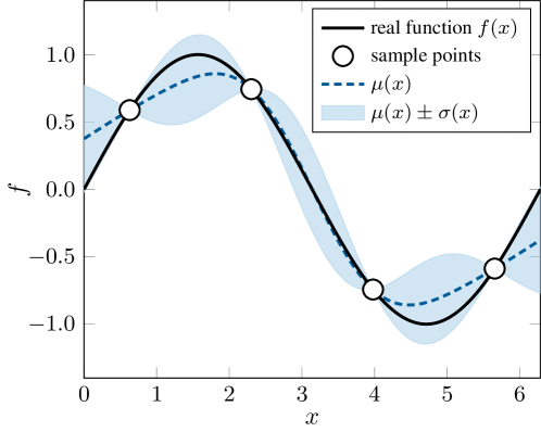
Figure 1: GP approximation of the $f=\sin(x)$ function.

The GP model of a one-dimensional function $f=\sin(x)$ is illustrated in Fig. 1. In this figure, the solid line represents the real function to be approximated, the circles represent the sample points, the dashed line represents the mean of the GP model and the filled area around the dashed line shows the standard derivation function of the GP model. We can see from the figure that the GP mean interpolates the samples. The standard derivation is zero at sample points and rises up between them.

2.2 Acquisition Function

After training the Gaussian process model, the next thing is to decide which point should be selected for expensive evaluation. The criterion for querying new samples is often called acquisition function or infill sampling function. Popular acquisition functions in Bayesian optimization are the expected improvement (EI) [4], probability of improvement (PI) [4], lower confidence bound (LCB) [4], knowledge gradient (KG) [43, 44], entropy search (ES) [45], predictive entropy search (PES) [46] and so on. Among them, EI is arguably the most widely used [47].

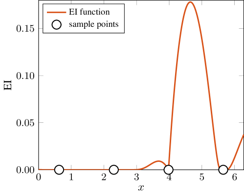
Figure 2: The EI function on the $f=\sin(x)$ problem.

Assume current best solution among the $n$ samples is $\bm{x}^{\star}$ and the corresponding minimum objective value is $f^{\star}=f(\bm{x}^{\star})$. The EI measures the expected value of improvement that the new point $\bm{x}$ can get beyond the current best solution $\bm{x}^{\star}$

$$\text{EI}(\bm{x})=\mathbb{E}\big{[}\max\big{(}f^{\star}-f(\bm{x}),0\big{)}\big{]}.$$ (7)

The closed-form expression can be derived using integration by parts [2]

$$\text{EI}(\bm{x})=\big{(}\mu(\bm{x})-f^{\star}\big{)}\Phi\bigg{(}\frac{\mu(\bm{x})-f^{\star}}{\sigma(\bm{x})}\bigg{)}+\sigma(\bm{x})\phi\bigg{(}\frac{\mu(\bm{x})-f^{\star}}{\sigma(\bm{x})}\bigg{)}$$ (8)

where $\Phi$ and $\phi$ are the cumulative and density distribution function of the standard Gaussian distribution respectively, and $\mu(\bm{x})$ and $\sigma(\bm{x})$ are the GP mean and standard deviation in (5) and (6) respectively.

The corresponding EI function of the GP model of the one-dimensional function is shown in Fig. 2. We can see that the EI function is multi-modal. The value is zero at sample points and rises up between different samples. In this simple example, the next point the EI function locates is very close to the global optimum point of the real function.

2.3 Bayesian Optimization

Often, Bayesian optimization (BO) starts with an initial design of experiment (DoE) to get a set of samples and evaluates these initial samples with the real objective function. Then, Bayesian optimization goes into the sequential optimization process. In each iteration, a GP model is trained using the samples in current data set. After that, a new point is located by optimizing an acquisition function, and then evaluated with the real objective function. This newly evaluated sample is then added to the data set. This iteration process stops when the maximum number of function evaluations is reached. The computational framework of Bayesian optimization can be summarized in Algorithm 1, where the EI acquisition function is used for example.

Algorithm 1 Computational Framework of BO

0:  $n_{\text{init}}=$ number of initial samples; $n_{\max}=$ maximum number of objective function evaluations.

0:  best found solution $(\bm{x}^{\star},f^{\star})$.

1:  Design of experiment: generate $n_{\text{init}}$ samples, evaluate them with the objective function, set current data set $\mathcal{D}=\{(\bm{x}^{(1)},f^{(1)}),\cdots,(\bm{x}^{(n_{\text{init}})},f^{(n_{\text{init}})})\}$, and set current number of evaluations $n=n_{\text{init}}$.

2:  Best solution setup: set current best solution as $\bm{x}^{\star}={\underset{1\leq i\leq n}{\arg\min}}f(\bm{x}^{(i)})$ and $f^{\star}={\underset{1\leq i\leq n}{\min}}f(\bm{x}^{(i)})$.

3:  while $n<n_{\max}$ do

4:     GP training: train a GP model using the current data set $\mathcal{D}$.

5:     Infill selection: locate a new point by maximizing the acquisition function

$$\bm{x}^{(n+1)}={\underset{\bm{x}\in\mathcal{X}}{\arg\max}}~{}\text{EI}(\bm{x}).$$

6:     Expensive evaluation: evaluate the new solution $f^{(n+1)}=f(\bm{x}^{(n+1)})$, update data set $\mathcal{D}=\{\mathcal{D},(\bm{x}^{(n+1)},f^{(n+1)})\}$, and update current number of evaluations $n=n+1$.

7:     Best solution update: update current best solution as $\bm{x}^{\star}={\underset{1\leq i\leq n}{\arg\min}}f(\bm{x}^{(i)})$ and $f^{\star}={\underset{1\leq i\leq n}{\min}}f(\bm{x}^{(i)})$.

8:  end while

As can be seen, in each iteration the new point is selected by maximizing the EI function which has the same dimension as the objective function. When the dimension of the problem is lower than 20, the EI maximum can be efficiently located by using state-of-the-art evolutionary algorithms. However, when the dimension of the problem goes up to near 100, locating a good point will be a great challenge. In addition, the EI function often has highly multi-modal surface with lots of flat regions, which makes searching the high-dimensional EI maximum more difficult.

3 Proposed Approach

In this work, we propose the expected coordinate improvement based Bayesian optimization (ECI-BO) algorithm to tackle this problem. Instead of searching the high-dimensional space for identifying a new point, we locate a new point by searching one coordinate at a time. Through iterates over all the coordinates, the original problem can be solved gradually. The proposed algorithm is introduced in detail in the following.

3.1 Expected Coordinate Improvement

First, we propose the expected coordinate improvement (ECI) criterion to measure how much improvement we can get along one coordinate. Assume $\bm{x}^{\star}$ is current best point and $f^{\star}$ is the corresponding current minimum objective. The ECI along the $i$th coordinate is

$$\text{ECI}_{i}(x)=\big{(}\mu(\bm{z})-f^{\star}\big{)}\Phi\bigg{(}\frac{\mu(\bm{z})-f^{\star}}{\sigma(\bm{z})}\bigg{)}+\sigma(\bm{z})\phi\bigg{(}\frac{\mu(\bm{z})-f^{\star}}{\sigma(\bm{z})}\bigg{)}$$ (9)

where $\bm{z}=[x_{1}^{\star},\cdots,x_{i-1}^{\star},x,x_{i+1}^{\star},\cdots,x_{d}^{\star}]$ has the same coordinates as the current best point $\bm{x}^{\star}$ except for the $i$th coordinate, which is the variable to be optimized.

In fact, the ECI function is a one-dimensional slice of the standard EI function while fixing all the other dimensions. A two-dimensional example is given in Fig. 3, where the surface is the standard EI function, the open circle is the current best point, and the two solid lines are the two ECI functions respectively. We can see that the $\text{ECI}_{1}(x)$ is the EI function fixing $x_{2}=x_{2}^{\star}$, and the $\text{ECI}_{2}(x)$ is the EI function fixing $x_{1}=x_{1}^{\star}$. As a result, the ECI function is able to measure the amount of improvement when we move the current best point along one coordinate.

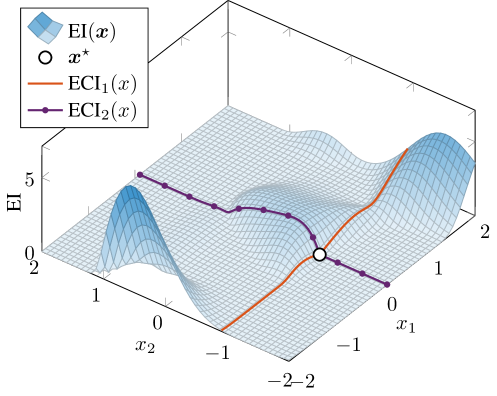
Figure 3: EI function and the corresponding ECI functions.

The major advantage of the proposed ECI function over the traditional EI function is that it is always a one-dimensional function no matter how many dimensions the original problem has. Therefore, the ECI function can be easily and efficiently optimized.

3.2 Expected Coordinate Improvement based Bayesian Optimization

Based on the ECI criterion, we propose the expected coordinate improvement based Bayesian optimization (ECI-BO) algorithm. The idea is to improve the current best point along one coordinate at a time, and iterates through all the coordinates as the optimization process goes on. To find the best order to optimize the coordinates, we use the maximal ECI values to approximately represent the effectiveness of the corresponding coordinates, and optimize the coordinates based on the order of their maximal ECI values. The computational framework of the proposed ECI-BO is given in Algorithm 2.

Algorithm 2 Computational Framework of the proposed ECI-BO

0:  $n_{\text{init}}=$ number of initial samples; $n_{\max}=$ maximum number of objective function evaluations.

0:  best found solution $(\bm{x}^{\star},f^{\star})$.

1:  Design of experiment: generate $n_{\text{init}}$ samples, evaluate them with the objective function, set current data set $\mathcal{D}=\{(\bm{x}^{(1)},f^{(1)}),\cdots,(\bm{x}^{(n_{\text{init}})},f^{(n_{\text{init}})})\}$, and set current number of evaluations $n=n_{\text{init}}$.

2:  Best solution setup: set current best solution as $\bm{x}^{\star}={\underset{1\leq i\leq n}{\arg\min}}f(\bm{x}^{(i)})$ and $f^{\star}={\underset{1\leq i\leq n}{\min}}f(\bm{x}^{(i)})$.

3:  while $n<n_{\max}$ do

4:     for $i=1$ to $d$ do

5:        Calculating maximal ECIs: Maximize the ECI function of the $i$th coordinate

$$\text{ECI}_{i,\max}=\max\text{ECI}_{i}(x)$$

6:     end for

7:     Sorting maximal ECIs: Sort the maximal ECI values in descending order to get the sorting indices

$$[r_{1},r_{2},\cdots,r_{d}]={\underset{1\leq i\leq d}{\arg\text{sort}}}~{}\text{ECI}_{i,\max}$$

8:     for $i=1$ to $d$ do

9:        GP training: train a GP model using the current data set $\mathcal{D}$.

10:        Infill selection: maximize the ECI function along the $r_{i}$ coordinate

$$x^{(n+1)}={\underset{a_{r_{i}}\leq x\leq b_{r_{i}}}{\arg\max}}\text{ECI}_{r_{i}}(x)$$

and form the new solution as

$$\bm{x}^{(n+1)}=[x_{1}^{\star},\cdots,x_{r_{i}-1}^{\star},x^{(n+1)},x_{r_{i}+1}^{\star},\cdots,x_{d}^{\star}].$$

11:        Expensive evaluation: evaluate the new solution $f^{(n+1)}=f(\bm{x}^{(n+1)})$, update data set $\mathcal{D}=\{\mathcal{D},(\bm{x}^{(n+1)},f^{(n+1)})\}$, and update current number of evaluations $n=n+1$.

12:        Best solution update: update current best solution as $\bm{x}^{\star}={\underset{1\leq i\leq n}{\arg\min}}f(\bm{x}^{(i)})$ and $f^{\star}={\underset{1\leq i\leq n}{\min}}f(\bm{x}^{(i)})$.

13:     end for

14:  end while

The key steps of the proposed ECI-BO algorithm are described in the following.

1. Design of experiment: in the first step, we generate $n_{\text{init}}$ initial samples using a design of experiment (DoE) method, such as Latin hypercube sampling method. After that, we evaluate these initial samples with the expensive objective function. In this step, these initial samples can be evaluated in parallel.

2. Best solution setup: the best solution of the initial samples is identified as $(\bm{x}^{\star},f^{\star})$.

3. Calculating maximal ECIs: before the acquisition function optimization process, we try to find the best order to optimize the coordinates. First, we maximize the ECI function of all the $d$ coordinates. Note that these $d$ optimization problems are all one-dimensional and can be executed in parallel.

4. Sorting maximal ECIs: After obtaining the maximal ECI values of all the coordinates, we sort the coordinates from the highest maximal ECI value to the lowest maximal ECI value, and set the coordinate optimization order as the sorting order. For example, if the maximal ECI values of a five-dimensional problems are $[200,300,500,400,100]$, then the coordinate optimization order is $\bm{r}=[3,4,2,1,5]$.

5. GP training: all the samples in current data set are used for training the GP model. We train the GP model in the original space instead of the one-dimensional subspace to ensure that the model has reasonable accuracy for the prediction.

6. Infill selection: in the $i$th iteration of the coordinate optimization process, we optimize the ECI function of the $r_{i}$th coordinate, where $r_{i}$ is the $i$th element of the previous obtained coordinate optimization order. Then, the infill solution is formed by replacing the $r_{i}$th coordinate of current best solution by the optimized value.

7. Expensive evaluation: the new infill solution is evaluated with the expensive objective function and this newly evaluated point is then added to the data set.

8. Best solution update: finally we update the best solution by considering the newly evaluated point. At this point, one coordinate optimization process is finished. Then, we move to the next coordinate and repeat the process from Step 9 to Step 12. Once all the coordinates has been covered, we go back to Step 4 to Step 7 to generate a new coordinate optimization order. This process continues until the maximum number of function evaluations is reached.

From the above process, we can find that the major difference between the proposed ECI-BO and the standard BO is that the proposed approach maximizes the one-dimensional ECI function to query a new point for expensive evaluation instead of the $d$-dimensional EI function. The one-dimensional ECI function is often significantly easier to solve than the $d$-dimensional EI function. Through iterating through all the coordinates, the original problem can be gradually solved.

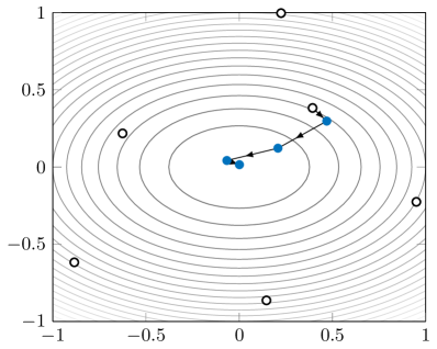
(a)

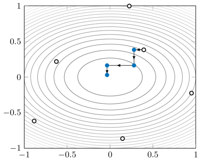
(b)

Figure 4: Search trajectories of the standard BO and the proposed ECI-BO on the Ellipsoid function. (a) standard BO. (b) proposed ECI-BO.

Since we move the current best solution along one coordinate at a time, the search trajectory of the proposed ECI-BO is very different from that of the standard BO. We plot the search trajectories of the standard BO and the proposed ECI-BO in Fig. 4(a) and Fig. 4(b), respectively, where the objective function is a simple two-dimensional Ellipsoid function $f=x_{1}^{2}+2x_{2}^{2}$, the open circles are six initial samples and the filled circles are four sequential infill samples. We can clearly see the difference in the search pattern between the standard BO and the proposed ECI-BO. In each iteration, the standard BO searches in the two-dimensional space to find the a new query point. In comparison, our proposed ECI-BO searches along one coordinate to locate a new point in one iteration. At the end of four iterations, both algorithms find solutions that are very close to the global optimum.

4 Numerical Experiments

In this section, we conduct numerical experiments to study the performance of our proposed ECI-BO algorithm. First, we compare our ECI-BO with the standard BO to see whether the proposed approach has improvement over the standard approach. Then, we compare the proposed ECI-BO with five high-dimensional BOs to see how well our algorithm performs when compared with the state-of-the-art approaches. A Matlab implementation of our ECI-BO is available at https://github.com/zhandawei/Expected_Coordinate_Improvement.

4.1 Experiment Settings

The settings of the numerical experiments are given in the following.

1. Test problems: the CEC 2017 test suit [48] is used for testing the compared algorithms. This test suit contains twenty-nine problems, in which $f_{1}$ and $f_{3}$ are unimodal problems, $f_{4}$ to $f_{10}$ are simple multimodal problems, $f_{11}$ to $f_{20}$ are hybrid problems, and $f_{21}$ to $f_{30}$ are composition problems. The problems in the test suite can well represent real-world problems. To test the competing algorithms’ ability to solve high-dimensional problems, the dimensions of the test problems are set to $d=100$ in the experiments.

2. Design of experiment: the Latin hypercube sampling (LHS) method is used for generating the initial samples. The number of initial samples is set to $n_{\text{init}}=200$ for all test problems.

3. Computation budget: the maximal number of function evaluations is set to $n_{\max}=1000$ for all test problems. This means the number of additional infill samples is then $n_{\max}-n_{\text{init}}=800$ for the test problems.

4. GP training: the squared exponential (SE) function is used as the kernel function for the GP model. The optimal hyperparameter of the SE kernel is found within $[0.01,100]$ using the sequential quadratic programming algorithm.

5. Infill selection: a real-coded genetic algorithm (GA) is applied to optimize the acquisition functions in the infill selection process. We use tournament selection for the parent selection, simulated binary crossover for the crossover and the ploynomial mutation for the mutation respectively in the GA. Both the distribution indices for crossover and mutation are set to 20. The number of acquisition function evaluations is set to $200d$ throughout the experiments. For the standard BO, the population size of the GA is set to 200 and the number of maximal generation is set to 100. For the proposed ECI-BO, the population size and the number of maximal generation are set to 10 and 20 respectively to maximize the 1-D ECI function.

6. Number of repetitions: all experiments are run 30 times with 30 different sets of initial samples. The initial design points are the same for different algorithms in one run but are different for different runs.

7. Experiment environment: all experiments are conducted on a Window 10 machine with an Intel i9-10900X CPU and 64 GB RAM.

In the first set of experiments, we compare the proposed ECI-BO with the standard BO. The optimization results of the two compared algorithms are given in Table 1, where the average and standard derivation values of 30 runs are shown. We conduct the Wilcoxon signed rank test with significance level of $\alpha=0.05$ to see whether the optimization results of the compared algorithms have significant difference. We use $+$, $-$ and $\approx$ to donate that the results of the proposed ECI-BO are significantly better than, worse than and similar to the results of the standard BO, respectively.

Table 1: Average and standard derivation results of the standard BO and the proposed ECI-BO

$f$	BO	ECI-BO
$f_{1}$	1.16E+10 (1.21E+09) $+$	2.76E+07 (8.03E+06)
$f_{3}$	1.58E+06 (2.01E+06) $\approx$	9.70E+05 (1.23E+05)
$f_{4}$	1.44E+04 (2.36E+03) $+$	3.37E+03 (6.83E+02)
$f_{5}$	1.61E+03 (5.71E+01) $+$	1.42E+03 (7.83E+01)
$f_{6}$	6.63E+02 (6.63E+00) $+$	6.12E+02 (3.25E+00)
$f_{7}$	2.23E+03 (7.47E+01) $+$	1.81E+03 (7.91E+01)
$f_{8}$	1.93E+03 (4.42E+01) $+$	1.71E+03 (1.03E+02)
$f_{9}$	4.45E+04 (8.01E+03) $-$	5.68E+04 (1.63E+04)
$f_{10}$	3.47E+04 (5.30E+02) $+$	1.75E+04 (1.96E+03)
$f_{11}$	4.71E+05 (1.07E+05) $+$	4.46E+05 (6.70E+05)
$f_{12}$	1.47E+10 (3.39E+09) $+$	7.49E+08 (3.12E+08)
$f_{13}$	4.54E+09 (1.50E+09) $+$	2.30E+08 (1.56E+08)
$f_{14}$	9.57E+07 (2.70E+07) $+$	7.20E+07 (2.90E+07)
$f_{15}$	3.41E+09 (7.67E+08) $+$	5.38E+08 (2.20E+08)
$f_{16}$	1.25E+04 (6.95E+02) $+$	1.05E+04 (4.63E+02)
$f_{17}$	9.17E+05 (7.52E+05) $-$	2.07E+06 (1.98E+06)
$f_{18}$	1.23E+08 (3.48E+07) $\approx$	1.06E+08 (5.51E+07)
$f_{19}$	2.84E+09 (9.24E+08) $+$	1.28E+08 (7.42E+07)
$f_{20}$	8.85E+03 (3.65E+02) $+$	6.04E+03 (7.41E+02)
$f_{21}$	3.57E+03 (5.34E+01) $+$	3.40E+03 (8.57E+01)
$f_{22}$	3.68E+04 (9.42E+02) $+$	1.96E+04 (1.61E+03)
$f_{23}$	4.17E+03 (5.06E+01) $+$	3.74E+03 (5.86E+01)
$f_{24}$	4.58E+03 (5.38E+01) $+$	4.29E+03 (8.35E+01)
$f_{25}$	1.18E+04 (1.21E+03) $+$	4.98E+03 (2.96E+02)
$f_{26}$	2.20E+04 (8.57E+02) $+$	1.81E+04 (1.13E+03)
$f_{27}$	4.57E+03 (1.50E+02) $+$	3.81E+03 (9.76E+01)
$f_{28}$	1.44E+04 (1.66E+03) $+$	8.81E+03 (3.34E+03)
$f_{29}$	4.46E+05 (3.09E+05) $\approx$	4.26E+05 (3.85E+05)
$f_{30}$	7.95E+09 (2.97E+09) $+$	1.19E+09 (4.25E+08)
$+$/$\approx$/$-$	24/3/2	N.A.

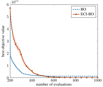
(a)

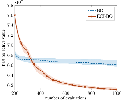
(b)

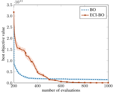
(c)

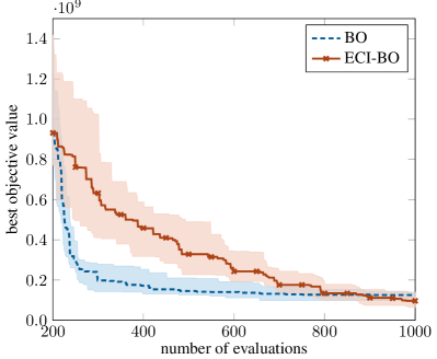
(d)

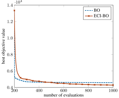
(e)

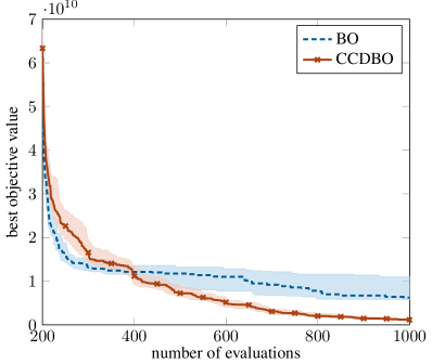
(f)

Figure 5: Convergence histories of the standard BO and the proposed ECI-BO on the test problems. (a) $f_{1}$. (b) $f_{6}$. (c) $f_{12}$. (d) $f_{18}$. (e) $f_{24}$. (f) $f_{30}$.

From the table we can see that our proposed ECI-BO obtains significantly better results than the standard BO on most of the test problems. For example, on the unimodal problem $f_{1}$, the average result found by the standard BO is 1.16E+10 while the average result found by the proposed ECI-BO is 2.76E+07. On the multimodal problem $f_{10}$ the numbers are 3.47E+04 and 1.75E+04, on the hybrid problem $f_{20}$ the numbers are 8.85E+03 and 6.04E+03, and on the composition problem $f_{30}$ the numbers are 7.95E+09 and 1.19E+09. Overall, our proposed ECI-BO finds better solutions on twenty-four test problems, worse solutions on two test problems and similar solutions on three test problems. The major difference between these two algorithms is that the proposed ECI-BO searches along one coordinate to find an infill solution in each iteration while the standard BO searches in the original design space for finding an infill solution. By iterating over the coordinates, our proposed ECI-BO is able to improve the solution gradually. At the end of 1000 evaluations, our proposed ECI-BO is able to find better solutions on most of the test problems. The experiment results can empirically prove the effectiveness of the proposed expected coordinate improvement approach.

The iteration histories of the two compared algorithms on six selected functions $f_{1}$, $f_{6}$, $f_{12}$, $f_{18}$, $f_{24}$ and $f_{30}$ are plotted in Fig. 5, where the horizontal axis is the number of function evaluations and the vertical axis is the current minimum objective value. The median, first quartile and the third quartile of the 30 runs are shown in the figures. From the iteration histories we can find a very interesting phenomenon. The standard BO converges faster than the proposed ECI-BO at the beginning of iterations, but converges slower than the proposed ECI-BO at the end of the iterations on most of the test problems. The standard BO searches in the original space to find new solutions while the proposed ECI-BO searches along one coordinate. Therefore, the standard BO is able to find better solutions than the ECI-BO at the beginning of the iterations. However, as the iteration goes on, most of the promising areas have been explored and exploitation is needed for further improvement. The standard BO still searches in the whole design space to find promising solutions, which often brings very little improvement as the iteration continues. On the contrary, the proposed ECI-BO searches along one coordinate at a time to find new solutions. Although it converges slower than the standard BO at the beginning of iterations when exploration is needed, it is able to continually find good solutions at the middle and at end of iterations when exploitation is urgently needed. At the end of iterations, the proposed ECI-BO often finds better solutions than the standard BO approach. Since the standard BO has faster convergence speed at the beginning of iterations, it is still preferred when the computation budget is extremely limited. But when the computation budget is fairly enough, the proposed ECI-BO should be preferred.

At last, we compare the computational time of the two algorithms. The computational time of them within one iteration consists of the time for training the GP model, the time for optimizing the acquisition function, and the time for evaluating the new point. The major difference between them is in optimizing the acquisition function. The proposed ECI-BO maximizes the 1-D ECI function to query a new point in each iteration while the standard BO maximizes the $d$-dimensional EI function to query a new point. As a result, the infill optimization problem of the proposed ECI-BO is often faster to solve than that of the standard BO algorithm. The running time of the two compared algorithms is plotted in Fig. 6, where the average computation time of 30 runs is shown. We can see that our proposed ECI-BO is significantly faster than the standard BO on 100-D problems. In summary, the proposed expected coordinate improvement approach is able to improve the standard Bayesian optimization algorithm’s optimization efficiency and reduce its computational cost at the same time.

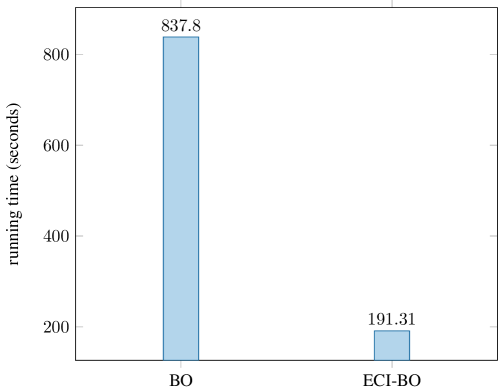
Figure 6: Running time of the proposed ECI-BO and the standard BO.

4.2 Comparison with High-dimensional BOs

To verify the effectiveness of the proposed approach, we compare our ECI-BO wit five high-dimensional BOs. The compared algorithms are described in the following.

1. Add-GP-UCB: The Add-GP-UCB algorithm [33] is the most popular high-dimensional BOs with the additive structural assumption. It decomposes the original problem into multiple low-dimensional sub-problems, solves these sub-problems and combines the solutions of the sub-problems into a high-dimensional solution. The low-dimensional space is also set to five in the experiments. The open source code of Add-GP-UCB  is used in the comparison.

2. Dropout: The Dropout approach [18] randomly selects a subset of variables to perform BO, and combine the solutions of the sub-problem with existing solutions to form a high-dimensional solution. Three different strategies for forming the high-dimensional solution are proposed in the work [18], and the copy strategy is used in the comparison. The dimension of the subspace is also set to five in the experiments. The open source code of the Dropout approach  is used in the comparison.

3. CoordinateLineBO: The CoordinateLineBO approach [39] randomly selects a coordinate to optimize in each iteration. The coordinates of the infill solution are the same as the current best solution except for the optimized coordinate. We implement the CoordinateLineBO algorithm in Matlab according to the work [39]. We use the genetic algorithm with population size of 10 and maximal generation of 20 to optimize the selected coordinate in each iteration for the CoordinateLineBO approach.

4. TuRBO: The TuRBO [37] uses the trust region approach to improve local search ability of Bayesian optimization algorithm on high-dimensional problems. The Thompson sampling is employed in TuRBO to select a batch of candidates to evaluate in each iteration. The number of trust regions is set to five and the number of batch evaluations is set to ten in the experiment. The open source code of TuRBO  is used in the comparison.

5. MCTS-VS: The MCTS-VS approach [19] is a high-dimensional BO with variable selection strategy. The Monte Carlo tree search method in employed iteratively to select a subset of variables to optimize in each iteration. The open source code of MCTS-VS  is used in the comparison.

The experiment results on the 100-D problems are shown in Table 2, where the average and standard deviation values of 30 runs are given. We also conduct Wilcoxon signed rank test, and use $+$, $-$ and $\approx$ to donate that our ECI-BO achieves significantly better, significantly worse and similar results compared with the competing algorithms.

Table 2: Average and standard derivation results of the compared high-dimensional BOs

$f$	Add-GP-UCB	Dropout	Coordinate LineBO	TuRBO	MCTR-VS	ECI-BO
$f_{1}$	2.35E+11 $+$	9.60E+10 $+$	4.20E+09 $+$	8.32E+10 $+$	1.39E+11 $+$	2.76E+07
$f_{3}$	4.45E+09 $\approx$	9.54E+05 $\approx$	9.63E+05 $\approx$	9.54E+05 $\approx$	2.36E+06 $+$	9.70E+05
$f_{4}$	7.09E+04 $+$	1.67E+04 $+$	6.81E+03 $+$	3.24E+04 $+$	2.51E+04 $+$	3.37E+03
$f_{5}$	2.21E+03 $+$	2.02E+03 $+$	1.69E+03 $+$	1.74E+03 $+$	1.67E+03 $+$	1.42E+03
$f_{6}$	7.24E+02 $+$	6.72E+02 $+$	6.42E+02 $+$	6.55E+02 $+$	6.60E+02 $+$	6.12E+02
$f_{7}$	4.49E+03 $+$	4.15E+03 $+$	2.35E+03 $+$	3.60E+03 $+$	4.73E+03 $+$	1.81E+03
$f_{8}$	2.58E+03 $+$	2.37E+03 $+$	2.05E+03 $+$	2.05E+03 $+$	1.96E+03 $+$	1.71E+03
$f_{9}$	9.13E+04 $+$	1.05E+05 $+$	8.26E+04 $+$	8.56E+04 $+$	5.02E+04 $\approx$	5.68E+04
$f_{10}$	3.29E+04 $+$	2.60E+04 $+$	2.30E+04 $+$	2.84E+04 $+$	3.42E+04 $+$	1.75E+04
$f_{11}$	7.04E+06 $+$	1.83E+05 $-$	2.89E+05 $-$	3.36E+05 $\approx$	4.52E+05 $+$	4.46E+05
$f_{12}$	2.14E+11 $+$	2.36E+10 $+$	4.05E+09 $+$	2.13E+10 $+$	5.25E+10 $+$	7.49E+08
$f_{13}$	4.46E+10 $+$	3.83E+09 $+$	1.68E+09 $+$	2.28E+09 $+$	1.10E+10 $+$	2.30E+08
$f_{14}$	3.49E+08 $+$	5.83E+07 $-$	9.01E+07 $+$	7.67E+07 $\approx$	1.30E+08 $+$	7.20E+07
$f_{15}$	3.03E+10 $+$	9.14E+08 $+$	1.60E+09 $+$	5.51E+08 $\approx$	5.06E+09 $+$	5.38E+08
$f_{16}$	1.53E+04 $+$	9.70E+03 $-$	1.14E+04 $+$	1.42E+04 $+$	1.27E+04 $+$	1.05E+04
$f_{17}$	3.98E+07 $+$	1.58E+04 $-$	1.89E+06 $\approx$	1.01E+05 $-$	3.60E+04 $-$	2.07E+06
$f_{18}$	6.86E+08 $+$	5.65E+07 $-$	1.08E+08 $\approx$	1.10E+08 $\approx$	2.61E+08 $+$	1.06E+08
$f_{19}$	2.93E+10 $+$	1.10E+09 $+$	9.95E+08 $+$	5.16E+08 $+$	5.78E+09 $+$	1.28E+08
$f_{20}$	8.63E+03 $+$	6.33E+03 $\approx$	7.09E+03 $+$	5.84E+03 $\approx$	8.45E+03 $+$	6.04E+03
$f_{21}$	4.19E+03 $+$	3.87E+03 $+$	3.56E+03 $+$	3.90E+03 $+$	3.59E+03 $+$	3.40E+03
$f_{22}$	3.60E+04 $+$	2.91E+04 $+$	2.44E+04 $+$	3.06E+04 $+$	3.64E+04 $+$	1.96E+04
$f_{23}$	5.06E+03 $+$	4.48E+03 $+$	3.93E+03 $+$	4.48E+03 $+$	4.22E+03 $+$	3.74E+03
$f_{24}$	6.38E+03 $+$	5.95E+03 $+$	4.50E+03 $+$	5.23E+03 $+$	5.26E+03 $+$	4.29E+03
$f_{25}$	2.40E+04 $+$	1.27E+04 $+$	7.08E+03 $+$	2.06E+04 $+$	1.99E+04 $+$	4.98E+03
$f_{26}$	3.86E+04 $+$	2.92E+04 $+$	1.95E+04 $+$	2.94E+04 $+$	2.40E+04 $+$	1.81E+04
$f_{27}$	7.14E+03 $+$	5.35E+03 $+$	4.01E+03 $+$	5.17E+03 $+$	5.19E+03 $+$	3.81E+03
$f_{28}$	2.38E+04 $+$	1.67E+04 $+$	1.50E+04 $+$	1.70E+04 $+$	2.22E+04 $+$	8.81E+03
$f_{29}$	6.25E+06 $+$	1.22E+04 $-$	2.18E+05 $-$	3.63E+04 $-$	2.76E+04 $-$	4.26E+05
$f_{30}$	4.00E+10 $+$	2.87E+09 $+$	2.26E+09 $+$	1.70E+09 $+$	7.78E+09 $+$	1.19E+09
$+$/$\approx$/$-$	28/1/0	21/2/6	24/3/2	21/6/2	26/1/2	N.A.

The Add-GP-UCB [33] assumes the objective function is a summation of multiple low-dimensional functions. However, the problems in CEC 2017 test suite do not meet this assumption. In comparison, our proposed ECI-BO does not make any structural assumption about the objective function we are optimizing. From Table 2, we can find that the Add-GP-UCB can not achieve satisfying results on the test problems. Our proposed ECI-BO performs significantly better than the Add-GP-UCB on twenty-eight of the twenty-nine problems.

The Dropout approach [18] randomly selects a few variables to optimize in each iteration. When evaluating the new solutions, this approach uses the values of existing points to fill the unselected variables. From the table we can find that our proposed ECI-BO performs significantly better on twenty-one problems, and significantly worse on six problems compared with the Dropout approach.

The CoordinateLineBO [39] is the most similar approach to our proposed ECI-BO. Both the CoordinateLineBO and our ECI-BO select one variable to optimize in each iteration. However, there are two major differences between them. First, our proposed algorithm iterates the coordinates over permutations while the the CoordinateLineBO iterates the coordinates randomly. When we iterates $d$ times, all the variables will be covered by the proposed approach, but some variables may not be covered by the CoordindateLineBO approach since some variables might be selected multiple times. Second, the CoordinateLineBO treats the variables equally, while our proposed ECI-BO learns the effectiveness of the variables based on their ECI values. The experiment results in Table 2 show that the proposed ECI-BO performs significantly better than the CoordinateLineBO approach on twenty-four problems. This can empirically prove the effectiveness of the proposed expected coordinate improvement approach.

The TuRBO [37] employees the trust region strategy in the BO framework to improve the local search ability of BO on high-dimensional problems. Compared with the TuRBO, our ECI-BO finds better solutions on twenty-one problems, similar solutions on six problems, and worse solutions on two problems. This means our proposed expected coordinate improvement approach is more effective than the trust region approach on the 100-D CEC 2017 test suite.

The MCTS-VS [19] is a recently developed variable selection strategy for high-dimensional Bayesian optimization. It employees the Monte Carlo tree search method to partition the variables into important and unimportant ones, and only optimizes the important variables [19]. The experiment results show that our proposed ECI-BO performs significantly better than the MCTS-VS approach on most of the test problems. This indicates that our ECI-BO is more suitable for problems whose variables are all effective to the objective function.

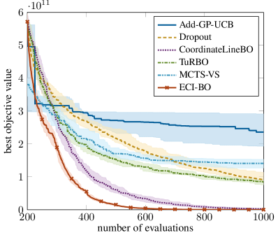
(a)

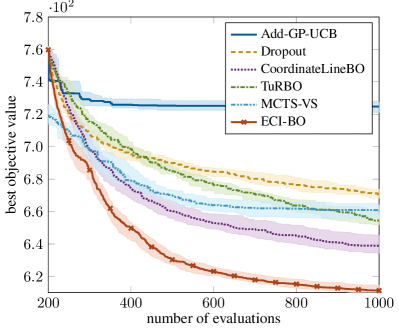
(b)

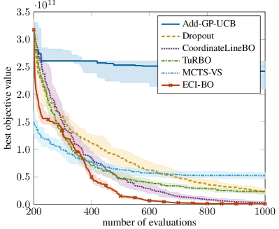
(c)

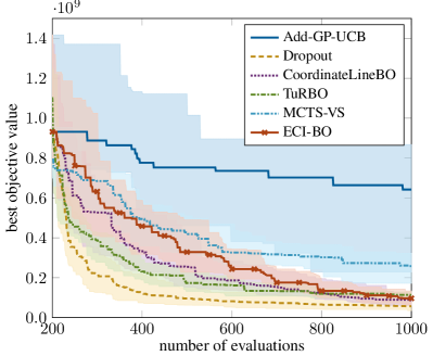
(d)

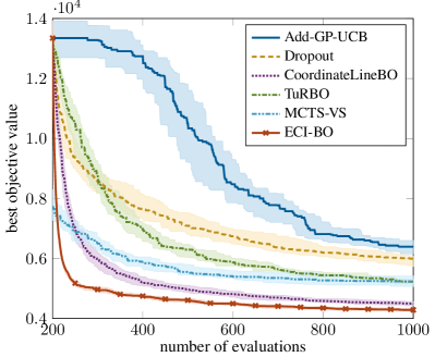
(e)

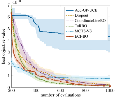
(f)

Figure 7: Convergence histories of the proposed ECI-BO and compared BOs on 100-D problems. (a) $f_{1}$. (b) $f_{6}$. (c) $f_{12}$. (d) $f_{18}$. (e) $f_{24}$. (f) $f_{30}$.

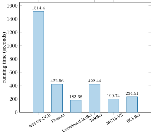
Figure 8: Running time of the proposed ECI-BO and compared high-dimensional BOs.

The convergence histories of the compared algorithms on six test problems are plotted in Fig. 7, where the median, first quartile and the third quartile of the 30 runs are shown. We can see that the proposed ECI-BO converges fastest and achieves the best results at the end of 1000 evaluations on $f_{1}$, $f_{6}$, $f_{12}$, $f_{24}$ and $f_{30}$ problems. The Dropout approach converges fastest and finds the best results on the $f_{18}$ problem, where the proposed ECI-BO achieves the second best results among the six compared algorithms.

The running time of the six compared BOs on the 100-D problem is plotted in Fig. 8, where the average values of 30 runs are shown. We can see that the CoordinateLineBO is the fastest approach while the Add-GP-UCB is the slowest approach among the six high-dimensional BOs. The Add-GP-UCB needs to train multiple low-dimensional GPs and optimize multiple acquisition functions in each iteration. While the other four approaches need only train one GP and optimize one acquisition function in each iteration. Therefore, the Add-GP-UCB is the most time-consuming approach among the six. Our proposed ECI-BO is faster than the Add-GP-UCB, Dropout and TurBO approaches, and is slightly slower than the CoordinateLineBO and MCTS-VS approaches. The only difference in computational time between our ECI-BO and the CoordinateLineBO is that our ECI-BO needs to maximize all the ECI functions to determine the coordinate optimization order before the infill optimization process. Therefore, our ECI-BO is slightly slower than the CoordinateLineBO. However, the additional computational time is around fifteen seconds, which can be neglected considering we are optimizing expensive problems.

5 Conclusions

In this work, we propose a simple and efficient approach to extend the Bayesian optimization algorithm to high-dimensional problems. We propose the expected coordinate improvement criterion to measure the amount of improvement we can get by moving the current best solution along one coordinate. Based on the expected coordinate improvement, we propose a high-dimensional Bayesian optimization approach which optimizes one coordinate at each iteration following the order of the coordinates’ expected coordinate improvement values. The proposed algorithm shows very competitive performance on the selected test suite when compared with the standard Bayesian optimization algorithm and five state-of-the-art high-dimensional approaches. Applying the expected coordinate improvement approach to multiobjective optimization would be very interesting work for future research.

References

- Mockus [1994] J. Mockus, Application of bayesian approach to numerical methods of global and stochastic optimization, Journal of Global Optimization 4 (1994) 347–365. doi:https://doi.org/10.1007/bf01099263.
- Jones et al. [1998] D. R. Jones, M. Schonlau, W. J. Welch, Efficient global optimization of expensive black-box functions, Journal of Global Optimization 13 (1998) 455–492. doi:https://doi.org/10.1023/A:1008306431147.
- Rasmussen and Williams [2006] C. E. Rasmussen, C. K. Williams, Gaussian processes for machine learning, The MIT Press, Cambridge, MA, USA, 2006.
- Jones [2001] D. R. Jones, A taxonomy of global optimization methods based on response surfaces, Journal of Global Optimization 21 (2001) 345–383. doi:https://doi.org/10.1023/A:1012771025575.
- Snoek et al. [2012] J. Snoek, H. Larochelle, R. P. Adams, Practical Bayesian optimization of machine learning algorithms, in: Advances in Neural Information Processing Systems, 2012, pp. 2951–2959.
- Shahriari et al. [2016] B. Shahriari, K. Swersky, Z. Wang, R. P. Adams, N. d. Freitas, Taking the human out of the loop: A review of bayesian optimization, Proceedings of the IEEE 104 (2016) 148–175. doi:https://doi.org/10.1109/JPROC.2015.2494218.
- Zhang et al. [2010] Q. Zhang, W. Liu, E. Tsang, B. Virginas, Expensive multiobjective optimization by MOEA/D with Gaussian process model, IEEE Transactions on Evolutionary Computation 14 (2010) 456–474. doi:https://doi.org/10.1109/TEVC.2009.2033671.
- Yang et al. [2019] K. Yang, M. Emmerich, A. Deutz, T. Bäck, Multi-objective bayesian global optimization using expected hypervolume improvement gradient, Swarm and Evolutionary Computation 44 (2019) 945–956. doi:https://doi.org/10.1016/j.swevo.2018.10.007.
- Han and Ouyang [2022] M. Han, L. Ouyang, A novel bayesian approach for multi-objective stochastic simulation optimization, Swarm and Evolutionary Computation 75 (2022) 101192. doi:https://doi.org/10.1016/j.swevo.2022.101192.
- Briffoteaux et al. [2020] G. Briffoteaux, M. Gobert, R. Ragonnet, J. Gmys, M. Mezmaz, N. Melab, D. Tuyttens, Parallel surrogate-assisted optimization: Batched bayesian neural network-assisted ga versus q-ego, Swarm and Evolutionary Computation 57 (2020) 100717. doi:https://doi.org/10.1016/j.swevo.2020.100717.
- Chen et al. [2023] J. Chen, F. Luo, G. Li, Z. Wang, Batch bayesian optimization with adaptive batch acquisition functions via multi-objective optimization, Swarm and Evolutionary Computation 79 (2023) 101293. doi:https://doi.org/10.1016/j.swevo.2023.101293.
- Zhan et al. [2023] D. Zhan, Y. Meng, H. Xing, A fast multipoint expected improvement for parallel expensive optimization, IEEE Transactions on Evolutionary Computation 27 (2023) 170–184. doi:https://doi.org/10.1109/TEVC.2022.3168060.
- Binois and Wycoff [2022] M. Binois, N. Wycoff, A survey on high-dimensional Gaussian process modeling with application to Bayesian optimization, ACM Transactions on Evolutionary Learning and Optimization 2 (2022) 1–26. doi:https://doi.org/10.1145/3545611.
- Linkletter et al. [2006] C. Linkletter, D. Bingham, N. Hengartner, D. Higdon, K. Q. Ye, Variable selection for gaussian process models in computer experiments, Technometrics 48 (2006) 478–490. doi:https://doi.org/10.1198/004017006000000228.
- Chen et al. [2012] B. Chen, R. M. Castro, A. Krause, Joint optimization and variable selection of high-dimensional Gaussian processes, in: International Conference on Machine Learning, 2012, p. 1379–1386.
- Zhang et al. [2023] F. Zhang, R.-B. Chen, Y. Hung, X. Deng, Indicator-based Bayesian variable selection for Gaussian process models in computer experiments, Computational Statistics & Data Analysis 185 (2023) 107757. doi:https://doi.org/10.1016/j.csda.2023.107757.
- Ulmasov et al. [2016] D. Ulmasov, C. Baroukh, B. Chachuat, M. P. Deisenroth, R. Misener, Bayesian optimization with dimension scheduling: Application to biological systems, Computer Aided Chemical Engineering 38 (2016) 1051–1056. doi:https://doi.org/10.1016/B978-0-444-63428-3.50180-6.
- Li et al. [2017] C. Li, S. Gupta, S. Rana, T. V. Nguyen, S. Venkatesh, A. Shilton, High dimensional Bayesian optimization using dropout, in: International Joint Conference on Artificial Intelligence, 2017, pp. 2096–2102.
- Song et al. [2022] L. Song, K. Xue, X. Huang, C. Qian, Monte carlo tree search based variable selection for high dimensional bayesian optimization, in: Advances in Neural Information Processing Systems, volume 35, 2022, pp. 28488–28501.
- Wang et al. [2016] Z. Wang, F. Hutter, M. Zoghi, D. Matheson, N. de Feitas, Bayesian optimization in a billion dimensions via random embeddings, Journal of Artificial Intelligence Research 55 (2016) 361–387. doi:https://doi.org/10.1613/jair.4806.
- Binois et al. [2015] M. Binois, D. Ginsbourger, O. Roustant, A warped kernel improving robustness in Bayesian optimization via random embeddings, in: International Conference on Learning and Intelligent Optimization, 2015, pp. 281–286. doi:https://doi.org/10.1007/978-3-319-19084-6_28.
- Nayebi et al. [2019] A. Nayebi, A. Munteanu, M. Poloczek, A framework for Bayesian optimization in embedded subspaces, in: International Conference on Machine Learning, volume 97, 2019, pp. 4752–4761.
- Binois et al. [2020] M. Binois, D. Ginsbourger, O. Roustant, On the choice of the low-dimensional domain for global optimization via random embeddings, Journal of Global Optimization 76 (2020) 69–90. doi:https://doi.org/10.1007/s10898-019-00839-1.
- Letham et al. [2020] B. Letham, R. Calandra, A. Rai, E. Bakshy, Re-examining linear embeddings for high-dimensional Bayesian optimization, in: Advances in Neural Information Processing Systems, volume 33, 2020, pp. 1546–1558.
- Papenmeier et al. [2022] L. Papenmeier, L. Nardi, M. Poloczek, Increasing the scope as you learn: Adaptive bayesian optimization in nested subspaces, in: Advances in Neural Information Processing Systems, 2022, pp. 11586–11601.
- Qian et al. [2016] H. Qian, Y.-Q. Hu, Y. Yu, Derivative-free optimization of high-dimensional non-convex functions by sequential random embeddings, in: International Joint Conference on Artificial Intelligence, 2016, pp. 1946–1952.
- Bouhlel et al. [2016] M. A. Bouhlel, N. Bartoli, A. Otsmane, J. Morlier, Improving Kriging surrogates of high-dimensional design models by partial least squares dimension reduction, Structural and Multidisciplinary Optimization 53 (2016) 935–952. doi:https://doi.org/10.1007/s00158-015-1395-9.
- Zhang et al. [2019] M. Zhang, H. Li, S. Su, High dimensional Bayesian optimization via supervised dimension reduction, in: International Joint Conference on Artificial Intelligence, 2019, pp. 4292–4298.
- Moriconi et al. [2020] R. Moriconi, M. P. Deisenroth, K. S. Sesh Kumar, High-dimensional bayesian optimization using low-dimensional feature spaces, Machine Learning 109 (2020) 1925–1943. doi:https://doi.org/10.1007/s10994-020-05899-z.
- Griffiths and Hernández-Lobato [2020] R.-R. Griffiths, J. M. Hernández-Lobato, Constrained Bayesian optimization for automatic chemical design using variational autoencoders, Chemical science 11 (2020) 577–586. doi:https://doi.org/10.1039/C9SC04026A.
- Siivola et al. [2021] E. Siivola, A. Paleyes, J. González, A. Vehtari, Good practices for Bayesian optimization of high dimensional structured spaces, Applied AI Letters 2 (2021) e24. doi:https://doi.org/10.1002/ail2.24.
- Maus et al. [2022] N. Maus, H. Jones, J. Moore, M. J. Kusner, J. Bradshaw, J. Gardner, Local latent space Bayesian optimization over structured inputs, in: Advances in Neural Information Processing Systems, volume 35, 2022, pp. 34505–34518.
- Kandasamy et al. [2015] T. Kandasamy, J. Schneider, B. Póczos, High dimensional Bayesian optimisation and bandits via additive models, in: International Conference on Machine Learning, 2015, p. 295–304.
- Li et al. [2016] C.-L. Li, K. Kandasamy, B. Poczos, J. Schneider, High dimensional Bayesian optimization via restricted projection pursuit models, in: International Conference on Artificial Intelligence and Statistics, volume 51, 2016, pp. 884–892.
- Rolland et al. [2018] P. Rolland, J. Scarlett, I. Bogunovic, V. Cevher, High-dimensional Bayesian optimization via additive models with overlapping groups, in: International Conference on Artificial Intelligence and Statistics, volume 84, 2018, pp. 298–307.
- Wang et al. [2017] Z. Wang, C. Li, S. Jegelka, P. Kohli, Batched high-dimensional Bayesian optimization via structural kernel learning, in: International Conference on Machine Learning, volume 70, 2017, pp. 3656–3664.
- Eriksson et al. [2019] D. Eriksson, M. Pearce, J. Gardner, R. D. Turner, M. Poloczek, Scalable global optimization via local Bayesian optimization, in: Advances in Neural Information Processing Systems, volume 32, 2019, pp. 5496–5507.
- Oh et al. [2018] C. Oh, E. Gavves, M. Welling, BOCK : Bayesian optimization with cylindrical kernels, in: International Conference on Machine Learning, volume 80, 2018, pp. 3868–3877.
- Kirschner et al. [2019] J. Kirschner, M. Mutny, N. Hiller, R. Ischebeck, A. Krause, Adaptive and safe Bayesian optimization in high dimensions via one-dimensional subspaces, in: International Conference on Machine Learning, volume 97, 2019, pp. 3429–3438.
- Frazier [2018] P. I. Frazier, A tutorial on Bayesian optimization, arXiv:.02811 (2018). doi:https://doi.org/10.48550/arXiv.1807.02811.
- Wang et al. [2023] X. Wang, Y. Jin, S. Schmitt, M. Olhofer, Recent advances in Bayesian optimization, ACM Computing Surveys 55 (2023) Article 287. doi:https://doi.org/10.1145/3582078.
- Forrester and Keane [2008] A. Forrester, A. Keane, Engineering design via surrogate modelling: a practical guide, John Wiley & Sons, 2008.
- Frazier et al. [2008] P. I. Frazier, W. B. Powell, S. Dayanik, A knowledge-gradient policy for sequential information collection, SIAM Journal on Control and Optimization 47 (2008) 2410–2439. doi:https://doi.org/10.1137/070693424.
- Frazier et al. [2009] P. Frazier, W. Powell, S. Dayanik, The knowledge-gradient policy for correlated normal beliefs, INFORMS Journal on Computing 21 (2009) 599–613. doi:https://doi.org/10.1287/ijoc.1080.0314.
- Hennig and Schuler [2012] P. Hennig, C. J. Schuler, Entropy search for information-efficient global optimization, Journal of Machine Learning Research 13 (2012) 1809–1837.
- Hernández-Lobato et al. [2014] J. M. Hernández-Lobato, M. W. Hoffman, Z. Ghahramani, Predictive entropy search for efficient global optimization of black-box functions, in: Advances in Neural Information Processing Systems, 2014, pp. 918–926.
- Zhan and Xing [2020] D. Zhan, H. Xing, Expected improvement for expensive optimization: a review, Journal of Global Optimization 78 (2020) 507–544. doi:https://doi.org/10.1007/s10898-020-00923-x.
- Awad et al. [2017] N. Awad, M. Ali, J. Liang, B. Qu, P. Suganthan, Problem definitions and evaluation criteria for the CEC special session and competition on single objective real-parameter numerical optimization, Technical Report, Technical Report, 2017.