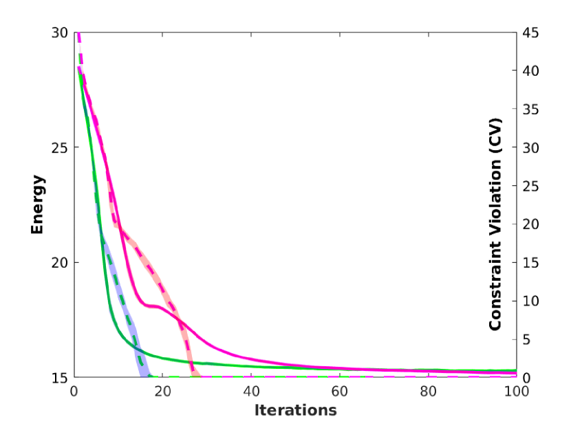
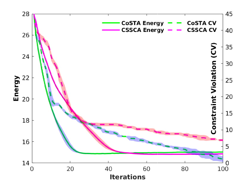
Constrained Stochastic Recursive Momentum Successive Convex Approximation

Basil M. Idrees, Lavish Arora, and Ketan Rajawat
Abstract

We consider stochastic optimization problems with functional constraints, such as those arising in trajectory generation, sparse approximation, and robust classification. If the objective and constraint functions are not convex, the classical stochastic approximation algorithms such as the proximal stochastic gradient descent do not lead to efficient algorithms. The non-convex constraints in particular, are handled via penalty methods, primal-dual approaches, or within the successive convex approximation (SCA) rubric. Still, constrained optimization problems are thought to be harder than the unconstrained ones, and existing approaches for solving such problems cannot match the stochastic first order (SFO)-complexity lower bound for minimization of general smooth functions.

In this work, we put forth an accelerated SCA algorithm that utilizes the recursive momentum-based acceleration which is widely used in the unconstrained setting. Remarkably, the proposed algorithm also achieves the optimal SFO complexity, at par with that achieved by state-of-the-art (unconstrained) stochastic optimization algorithms. At each iteration, the proposed algorithm entails constructing convex surrogates of the objective and the constraint functions, and solving the resulting convex optimization problem. A recursive update rule is employed to track the gradient of the objective function, and contributes to achieving faster convergence and improved SFO complexity. A key ingredient of the proof is a new parameterized version of the standard Mangasarian-Fromowitz Constraints Qualification, that allows us to bound the dual variables and hence establish that the iterates approach an ϵitalic-ϵ\epsilon-stationary point. We also detail a obstacle-avoiding trajectory optimization problem that can be solved using the proposed algorithm, and show that its performance is superior to that of the existing algorithms. The performance of the proposed algorithm is also compared against that of a specialized sparse classification algorithm on a binary classification problem.

I Introduction

I-A Background

In this work, we consider the stochastic non-convex constrained optimization problem:

F=min𝐱nsuperscript𝐹subscript𝐱superscript𝑛\displaystyle F^{\star}=\min_{{\mathbf{x}}\in{\mathbb{R}}^{n}} F(𝐱):=U(𝐱)+u(𝐱)assign𝐹𝐱𝑈𝐱𝑢𝐱\displaystyle~{}F({\mathbf{x}}):=U({\mathbf{x}})+u({\mathbf{x}}) (𝒫𝒫\mathcal{P})
s. t. hi(𝐱)0,subscript𝑖𝐱0\displaystyle~{}~{}~{}~{}~{}~{}h_{i}({\mathbf{x}})\leq 0, i=1,,I𝑖1𝐼\displaystyle i=1,\ldots,I
gj(𝐱)0,subscript𝑔𝑗𝐱0\displaystyle~{}~{}~{}~{}~{}~{}g_{j}({\mathbf{x}})\leq 0, j=1,,J𝑗1𝐽\displaystyle j=1,\ldots,J

where U(𝐱):=𝔼[f(𝐱,𝝃)]assign𝑈𝐱𝔼delimited-[]𝑓𝐱𝝃U({\mathbf{x}}):={\mathbb{E}}[f({\mathbf{x}},{\boldsymbol{\xi}})] and f𝑓f is a smooth possibly non-convex function, while {gj}j=1Jsuperscriptsubscriptsubscript𝑔𝑗𝑗1𝐽\{g_{j}\}_{j=1}^{J} are smooth but possibly non-convex functions. On the other hand, the functions {hi}i=1Isuperscriptsubscriptsubscript𝑖𝑖1𝐼\{h_{i}\}_{i=1}^{I} are smooth convex functions, and u𝑢u is a convex function. Here, the expectation is with respect to the random variable 𝝃𝝃{\boldsymbol{\xi}} with an unknown distribution. We seek to solve (𝒫𝒫\mathcal{P}) using stochastic approximation schemes that require independent samples of 𝝃𝝃{\boldsymbol{\xi}} observed sequentially over time.

Non-convex constrained optimization problems routinely arise in a number of areas, including robotics, machine learning, and signal processing. For instance, trajectory generation, target tracking, navigation, and path planning problems can often be cast as non-convex optimization problems [1, 2, 3, 4, 5] with non-convex obstacle-avoidance or boundary constraints. Similarly in supervised machine learning, constraints are often imposed ensure the resulting models are both robust and fair[6, 7]. Constraints may also be imposed to incorporate prior knowledge of the problem at hand, such as to ensure that the learned features are sparse in some domain [8].

Existing approaches to solve (𝒫𝒫\mathcal{P}) include the primal-dual method [9], penalty method [10], proximal point methods [11, 12], and several Sucessive Convex Approximation (SCA) variants [13, 14, 15, 16, 17]. The performance of these algorithms is usually measured in terms of their oracle complexity, which is the number of calls to the stochastic first-order (SFO) oracle required to reach a point that satisfies the Karush-Kuhn Tucher (KKT) conditions to within a tolerance of ϵitalic-ϵ\epsilon. The primal-dual method proposed in [9] iteratively updates both primal and dual variables based on a stochastic approximation to augmented Lagrangian function, achieving an oracle complexity of 𝒪(ϵ2.5)𝒪superscriptitalic-ϵ2.5\mathcal{O}(\epsilon^{-2.5}). An improved rate of 𝒪(ϵ2)𝒪superscriptitalic-ϵ2\mathcal{O}(\epsilon^{-2}) is achieved by [10] which utilizes a penalty functional to reformulate (𝒫𝒫\mathcal{P}) as an unconstrained optimization problem. The same rate is also achieved by the proximal point method ConEx [12] and level-constrained stochastic proximal gradient (LCSPG) method [11], both of which solve a sequence of strongly convex subproblems, obtained by adding a quadratic term to the objective and constraint functions. A related level-constrained proximal point (LCPP) method [8] also achieved the same rate but was customized to only handle sparsity inducing constraint functions.

Different from these approaches, SCA represents a more flexible framework for solving generic non-convex constrained optimization problems. It is an iterative approach, where at every iteration, the non-convex objective and constraint functions are replaced with their convex surrogates, tailored to the problem at hand [18, 19]. Stochastic SCA variants have been proposed in [20, 13, 14, 15, 16, 17] for solving (𝒫𝒫\mathcal{P}) as well as its more general version with stochastic constraints. These works however only report asymptotic convergence results, and do not provide a comprehensive oracle complexity analysis. Non-asymptotic rates are only known for the classical SCA algorithm when solving the deterministic version of (𝒫𝒫\mathcal{P}) with convex constraints [21, 22, 23, 24], where the latter work achieved the state-of-the-art rate of 𝒪(ϵ2)𝒪superscriptitalic-ϵ2\mathcal{O}(\epsilon^{-2}).

We remark that the oracle complexity of 𝒪(ϵ2)𝒪superscriptitalic-ϵ2{\mathcal{O}}(\epsilon^{-2}) achieved by various algorithms that solve (𝒫𝒫\mathcal{P}) is not optimum [25]. Indeed, using momentum or variance reduction techniques [26, 27, 28, 29, 30], it is well-known that the optimal oracle complexity of 𝒪(ϵ3/2)𝒪superscriptitalic-ϵ32\mathcal{O}(\epsilon^{-3/2}) can be achieved for unconstrained or convex-constrained version of (𝒫𝒫\mathcal{P}). Interestingly, variance reduction is applied to the level-constrained proximal algorithm in [11] for finite-sum problems but the rate achieved is only 𝒪(ϵ2)𝒪superscriptitalic-ϵ2{\mathcal{O}}(\epsilon^{-2}), with a remark that it can be improved to 𝒪(ϵ3/2)𝒪superscriptitalic-ϵ32\mathcal{O}(\epsilon^{-3/2}) if the objective is assumed to be smooth, but without any proof [11, Remark 5].

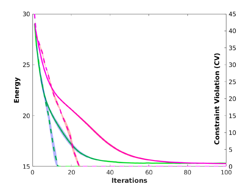
In this work, we incorporate STOchastic Recursive Momentum (STORM) updates from [31, 26] within the SCA framework to achieve the optimum rate of 𝒪(ϵ3/2)𝒪superscriptitalic-ϵ32\mathcal{O}(\epsilon^{-3/2}). The proposed Constrained STORM SCA (CoSTA) algorithm uses momentum-enhanced surrogates with adaptive step-sizes in the spirit of [31, 26]. We also establish that the empirical performance of the proposed algorithm is better than that of CSSCA [13], which does not use momentum or variance-reduction, and at par with LCPP [8], which can only handle sparsity-inducing constraints.

Before concluding this section, we remark that analysis of optimization problems with non-convex constraints inevitably requires some assumptions called the constraint qualifications (CQ). These CQs are essential regularity conditions that ensure that the constraint functions are well-behaved, so that the intermediate updates or subproblems are well-defined. Technically, these CQs are utilized to ensure that the intermediate dual variables remain bounded across iterations. Commonly used CQs include the Non-singularity condition (NSC) [9], Linear Independence CQ (LICQ) [32], Linear Independence regularity condition (LIRC) [17], and most commonly the Mangasarian-Fromovitz CQ (MFCQ) condition [12, 11, 8]. It was observed in [11, Sec. 3.1] that the classical MFCQ only implies the existance of a bound B𝐵B on the dual variables, but does not relate B𝐵B to the other problem parameters, leaving the possibility of B𝐵B getting arbitrarily large. It was suggested in [11] to use a stronger CQ such as the strong feasibility CQ (SFCQ) so as to ensure a problem parameter-dependent oracle complexity bound. In this work, we instead utilize a stronger parameterized version of MFCQ to the same effect, i.e., bound the dual variables in terms of problem-dependent quantities.

Table I summarizes the comparative performance of various state-of-the-art algorithms that can be used to solve (𝒫𝒫\mathcal{P}). We observe that the optimal rate is achieved only by the proposed CoSTA algorithm. Additional remarks on CQ and algorithm structure also included.

TABLE I: Comparison of the complexity results of several algorithms in literature to our algorithm to produce a stochastic ϵitalic-ϵ\epsilon-stationary solution of constrained stochastic non-convex optimization problem (To make the comparisons fair we have converted the oracle complexity results of the all the works to match our definition of (17)-(19))
Reference Rate
Constraint
Qualification
Remarks
CoSTA
(This work)
𝓞(ϵ𝟑/𝟐)𝓞superscriptbold-italic-ϵ32\boldsymbol{\mathcal{O}(\epsilon^{-3/2})} Strong MFCQ SCA-based
CSSCA [13],
SSCA [15]
-
Slater’s condition established
for limit points
Asymptotic convergence proved
ConEx [12] 𝒪(ϵ2)𝒪superscriptitalic-ϵ2\mathcal{O}(\epsilon^{-2})
MFCQ / SFCQ
SCA-based
Stochastic Primal-
Dual SGM [9]
𝒪(ϵ2.5)𝒪superscriptitalic-ϵ2.5\mathcal{O}(\epsilon^{-2.5}) NSC Dual variables also updated
LCSPG [11] 𝒪(ϵ2)𝒪superscriptitalic-ϵ2\mathcal{O}(\epsilon^{-2})
MFCQ / SFCQ
Remark 5 mentions that
improved rates are possible.
LCPP[8] 𝒪(ϵ2)𝒪superscriptitalic-ϵ2\mathcal{O}(\epsilon^{-2}) MFCQ For sparsity-constrained problems only

I-B Notations

The lower case letter are used for denoting scalars while bold lower case letters are used for denoting vectors. Also, bold upper case letters are used for denoting matrices. For a matrix 𝐀𝐀{\mathbf{A}}, diag(𝐚)𝑑𝑖𝑎𝑔𝐚diag({\mathbf{a}}) is used to denote diagonal matrix with elements (a1,a2,ak)subscript𝑎1subscript𝑎2subscript𝑎𝑘(a_{1},a_{2},\ldots a_{k}). We collect the functions {gj}j=1Jsuperscriptsubscriptsubscript𝑔𝑗𝑗1𝐽\{g_{j}\}_{j=1}^{J} and {hi}i=1Isuperscriptsubscriptsubscript𝑖𝑖1𝐼\{h_{i}\}_{i=1}^{I} into vector-valued functions 𝐠:nJ:𝐠superscript𝑛superscript𝐽{\mathbf{g}}:{\mathbb{R}}^{n}\rightarrow{\mathbb{R}}^{J} and 𝐡:nI:𝐡superscript𝑛superscript𝐼{\mathbf{h}}:{\mathbb{R}}^{n}\rightarrow{\mathbb{R}}^{I}, respectively. Binary operators such as \leq and \geq when applied to vectors are interpreted entry-wise, i.e., 𝐠(𝐱)0𝐠𝐱0{\mathbf{g}}({\mathbf{x}})\leq 0 means gj(𝐱)0subscript𝑔𝑗𝐱0g_{j}({\mathbf{x}})\leq 0 for all 1jJ1𝑗𝐽1\leq j\leq J. We denote 𝐠(𝐱)=[g1(𝐱)gJ(𝐱)]𝖳𝐠𝐱superscriptmatrixsubscript𝑔1𝐱subscript𝑔𝐽𝐱𝖳\nabla{\mathbf{g}}({\mathbf{x}})=\begin{bmatrix}\nabla g_{1}({\mathbf{x}})&\ldots\nabla g_{J}({\mathbf{x}})\end{bmatrix}^{\mathsf{T}}.

The rest of the paper is organized as follows. In Sec II we present an example that motivate the problem at hand. In Section III the problem statement is posed along with the proposed algorithm. In Section IV a non-asymptotic convergence analysis of the CoSTA algorithm is detailed. Section V briefly describes the potential application of CoSTA. Finally, Section VI the conclusion is provided.

II Motivating Examples

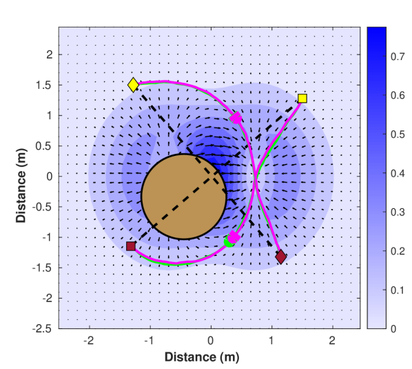
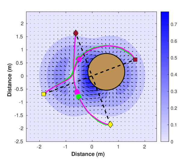
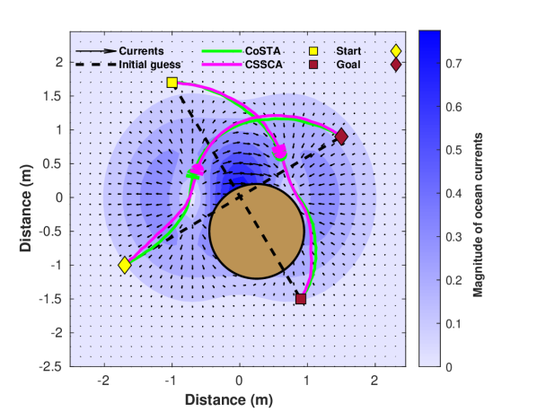
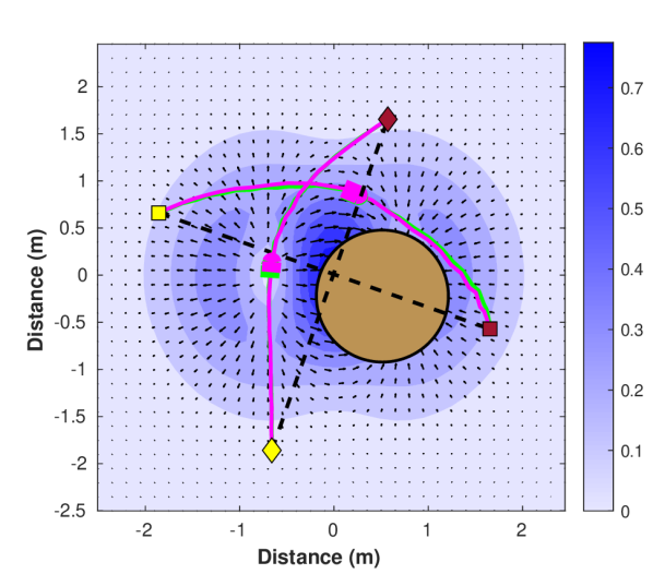
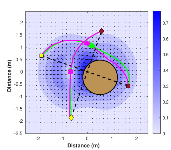
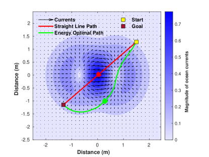
In this section, we discuss a variant of the widely studied Zermelo’s navigation problem [33], and formulate it as an instance of (𝒫𝒫\mathcal{P}). Consider a surface vehicle in an ocean environment that seeks to traverse from one point to another, while using minimal energy. If the ocean currents are known ahead of time, the vehicle may save energy by moving along the flows instead of moving along the straight line from the source to the destination. An example is depicted in Fig. 1, where the straight line path (shown in red) incurs an energy of 14.8 J while the energy-optimal path (shown in green) requires only 8.5 J.
Refer to caption
Figure 1: Navigation under ocean currents. The green energy-optimal path harnesses the currents by judiciously applying control effort as the vehicle drifts along towards the goal, achieving lower energy (8.5 J) compared to the straight line path (14.8 J).

In practice however, the ocean currents in a given region 2superscript2{\mathcal{B}}\subset{\mathbb{R}}^{2}, denoted by ϑ(𝐱)italic-ϑ𝐱\vartheta({\mathbf{x}}) m/s for each 𝐱𝐱{\mathbf{x}}\in{\mathcal{B}}, cannot be accurately predicted. Instead, various meteorological or oceanographic agencies [34, 35, 36, 37] employ ensemble forecasting, a technique that captures the measurement uncertainty inherent to the prediction process, by providing a range of possible ocean current forecasts [38, 39]. Mathematically, an instance of the ensemble forecast can be denoted by {ϑ(𝐱,𝝃)}𝐱subscriptitalic-ϑ𝐱𝝃𝐱\{\vartheta({\mathbf{x}},{\boldsymbol{\xi}})\}_{{\mathbf{x}}\in{\mathcal{B}}} where 𝝃𝝃{\boldsymbol{\xi}} is the index of a member of the ensemble. It has been observed that summary statistics, such as the average currents, cannot generally be used for path planning, as these may yield sub-optimal and potentially unsafe trajectories [40]. Instead, the ensemble forecasts should be directly employed to obtain trajectories that minimize the average energy.

In this work, we consider the problem of designing the energy-optimal trajectories of N𝑁N agents, while avoiding an obstacle. Mathematically, the problem entails finding a collection of T𝑇T waypoints {𝐱i(τ)}τ=1Tsuperscriptsubscriptsubscript𝐱𝑖𝜏𝜏1𝑇\{{\mathbf{x}}_{i}(\tau)\}_{\tau=1}^{T} for each agent i𝑖i, collected in the super-vector 𝐱¯2NT¯𝐱superscript2𝑁𝑇\underline{{\mathbf{x}}}\in{\mathbb{R}}^{2NT}. The waypoints are equally spaced at intervals of Δt=Tf/TΔ𝑡subscript𝑇𝑓𝑇\Delta t=T_{f}/T seconds where Tfsubscript𝑇𝑓T_{f} is the given time horizon. The i𝑖i-th agent starts at a given location 𝐱i(0)subscript𝐱𝑖0{\mathbf{x}}_{i}(0) and wants to reach the goal location 𝐱igsuperscriptsubscript𝐱𝑖𝑔{\mathbf{x}}_{i}^{g}, such that 𝐱i(T)=𝐱igsubscript𝐱𝑖𝑇superscriptsubscript𝐱𝑖𝑔{\mathbf{x}}_{i}(T)={\mathbf{x}}_{i}^{g}. For collision avoidance, we assume that the agents and the obstacle have a circular shape with radii r𝑟r and rosuperscript𝑟𝑜r^{o}, respectively. Finally, consider the agent’s movement from 𝐱i(τ)subscript𝐱𝑖𝜏{\mathbf{x}}_{i}(\tau) to 𝐱i(τ+1)subscript𝐱𝑖𝜏1{\mathbf{x}}_{i}(\tau+1), where 0τT10𝜏𝑇10\leq\tau\leq T-1. The control input — and consequently, the energy — can be considered proportional to the quantity 𝐱i(τ+1)𝐱i(τ)ϑ(𝐱i(τ),𝝃)Δt2superscriptnormsubscript𝐱𝑖𝜏1subscript𝐱𝑖𝜏italic-ϑsubscript𝐱𝑖𝜏𝝃Δ𝑡2\left\|{\mathbf{x}}_{i}(\tau+1)-{\mathbf{x}}_{i}(\tau)-\vartheta({\mathbf{x}}_{i}(\tau),{\boldsymbol{\xi}})\Delta t\right\|^{2}. Here, the term ϑ(𝐱i(τ),𝝃)Δtitalic-ϑsubscript𝐱𝑖𝜏𝝃Δ𝑡\vartheta({\mathbf{x}}_{i}(\tau),{\boldsymbol{\xi}})\Delta t approximates the vehicle’s displacement without any control input. Hence, the vehicle should seek to minimize the cumulative energy input while ensuring that the magnitude of the control input does not exceed the vehicle specifications, denoted by vimaxsuperscriptsubscript𝑣𝑖v_{i}^{\max}. In summary, the considered problem can be written as

min𝐱¯subscript¯𝐱\displaystyle\min_{\underline{{\mathbf{x}}}} i=1Nτ=0T1𝔼[𝐱i(τ+1)𝐱i(τ)ϑ(𝐱i(τ),𝝃)Δt2]superscriptsubscript𝑖1𝑁superscriptsubscript𝜏0𝑇1𝔼delimited-[]superscriptnormsubscript𝐱𝑖𝜏1subscript𝐱𝑖𝜏italic-ϑsubscript𝐱𝑖𝜏𝝃Δ𝑡2\displaystyle\sum_{i=1}^{N}\sum_{\tau=0}^{T-1}{\mathbb{E}}[\left\|{\mathbf{x}}_{i}(\tau+1)-{\mathbf{x}}_{i}(\tau)-\vartheta({\mathbf{x}}_{i}(\tau),{\boldsymbol{\xi}})\Delta t\right\|^{2}] (1a)
s. t. 𝐱i(T)=𝐱igsubscript𝐱𝑖𝑇subscriptsuperscript𝐱𝑔𝑖\displaystyle{\mathbf{x}}_{i}(T)={\mathbf{x}}^{g}_{i} (1b)
𝐱i(τ)𝐱oro+r,τ,inormsubscript𝐱𝑖𝜏superscript𝐱𝑜superscript𝑟𝑜𝑟for-all𝜏𝑖\displaystyle\left\|{\mathbf{x}}_{i}(\tau)-{\mathbf{x}}^{o}\right\|\geq r^{o}+r,\hskip 28.45274pt\forall~{}\tau,i (1c)
𝐱i(τ)𝐱j(τ)2r,τ,ijformulae-sequencenormsubscript𝐱𝑖𝜏subscript𝐱𝑗𝜏2𝑟for-all𝜏𝑖𝑗\displaystyle\left\|{\mathbf{x}}_{i}(\tau)-{\mathbf{x}}_{j}(\tau)\right\|\geq 2r,\hskip 28.45274pt\forall~{}\tau,i\neq j (1d)
𝐱i(τ+1)𝐱i(τ)ϑ(𝐱i(τ),𝝃)ΔtvimaxΔtτ,i,𝝃normsubscript𝐱𝑖𝜏1subscript𝐱𝑖𝜏italic-ϑsubscript𝐱𝑖𝜏𝝃Δ𝑡superscriptsubscript𝑣𝑖Δ𝑡for-all𝜏𝑖𝝃\displaystyle\left\|{\mathbf{x}}_{i}(\tau+1)-{\mathbf{x}}_{i}(\tau)-\vartheta({\mathbf{x}}_{i}(\tau),{\boldsymbol{\xi}})\Delta t\right\|\leq v_{i}^{\max}\Delta t\hskip 5.69054pt\forall~{}\tau,i,{\boldsymbol{\xi}} (1e)

where the objective seeks to minimize the cumulative energy consumption averaged over the given ensembles, (1b) enforces the termination condition, (1c)-(1d) ensure that the vehicles maintain safe distances from each other and from the obstacle, and (1e) limits the maximum control input for every agent, time, and realization. Of these, (1e) contains an impractically large number of constraints, one for each realization, and renders the problem difficult to solve. To avoid this issue, we consider a more stringent reformulation of the constraint that implies (1e). To this end, we assume that the ensemble forecasts have a uniformly bounded support, i.e., ϑ(𝐱,𝝃)𝔼[ϑ(𝐱,𝝃)]Δϑmaxnormitalic-ϑ𝐱𝝃𝔼delimited-[]italic-ϑ𝐱𝝃Δsuperscriptitalic-ϑ\left\|\vartheta({\mathbf{x}},{\boldsymbol{\xi}})-{\mathbb{E}}\left[\vartheta({\mathbf{x}},{\boldsymbol{\xi}})\right]\right\|\leq\Delta\vartheta^{\max} for 𝐱𝐱{\mathbf{x}}\in{\mathcal{B}}. Introducing 𝔼[ϑ(𝐱i(τ),𝝃)]Δt𝔼delimited-[]italic-ϑsubscript𝐱𝑖𝜏𝝃Δ𝑡{\mathbb{E}}\left[\vartheta({\mathbf{x}}_{i}(\tau),{\boldsymbol{\xi}})\right]\Delta t inside the norm on the left of (1e) and using the triangle inequality, we observe that

𝐱i(τ+1)𝐱i(τ)ϑ(𝐱i(τ),𝝃)Δtnormsubscript𝐱𝑖𝜏1subscript𝐱𝑖𝜏italic-ϑsubscript𝐱𝑖𝜏𝝃Δ𝑡\displaystyle\left\|{\mathbf{x}}_{i}(\tau+1)-{\mathbf{x}}_{i}(\tau)-\vartheta({\mathbf{x}}_{i}(\tau),{\boldsymbol{\xi}})\Delta t\right\| (2)
𝐱i(τ+1)𝐱i(τ)𝔼[ϑ(𝐱i(τ),𝝃)]Δtabsentnormsubscript𝐱𝑖𝜏1subscript𝐱𝑖𝜏𝔼delimited-[]italic-ϑsubscript𝐱𝑖𝜏𝝃Δ𝑡\displaystyle\leq\left\|{\mathbf{x}}_{i}(\tau+1)-{\mathbf{x}}_{i}(\tau)-{\mathbb{E}}\left[\vartheta({\mathbf{x}}_{i}(\tau),{\boldsymbol{\xi}})\right]\Delta t\right\|
+Δtϑ(𝐱i(τ),𝝃)𝔼[ϑ(𝐱i(τ),𝝃)]Δ𝑡normitalic-ϑsubscript𝐱𝑖𝜏𝝃𝔼delimited-[]italic-ϑsubscript𝐱𝑖𝜏𝝃\displaystyle+\Delta t\left\|\vartheta({\mathbf{x}}_{i}(\tau),{\boldsymbol{\xi}})-{\mathbb{E}}\left[\vartheta({\mathbf{x}}_{i}(\tau),{\boldsymbol{\xi}})\right]\right\|
𝐱i(τ+1)𝐱i(τ)𝔼[ϑ(𝐱i(τ),𝝃)]Δt+ΔϑmaxΔt.absentnormsubscript𝐱𝑖𝜏1subscript𝐱𝑖𝜏𝔼delimited-[]italic-ϑsubscript𝐱𝑖𝜏𝝃Δ𝑡Δsuperscriptitalic-ϑΔ𝑡\displaystyle\leq\left\|{\mathbf{x}}_{i}(\tau+1)-{\mathbf{x}}_{i}(\tau)-{\mathbb{E}}\left[\vartheta({\mathbf{x}}_{i}(\tau),{\boldsymbol{\xi}})\right]\Delta t\right\|+\Delta\vartheta^{\max}\Delta t.

Hence, the constraint

𝐱i(τ+1)𝐱i(τ)𝔼[ϑ(𝐱i(τ),𝝃)]Δtnormsubscript𝐱𝑖𝜏1subscript𝐱𝑖𝜏𝔼delimited-[]italic-ϑsubscript𝐱𝑖𝜏𝝃Δ𝑡\displaystyle\left\|{\mathbf{x}}_{i}(\tau+1)-{\mathbf{x}}_{i}(\tau)-{\mathbb{E}}\left[\vartheta({\mathbf{x}}_{i}(\tau),{\boldsymbol{\xi}})\right]\Delta t\right\| (vimaxΔϑmax)Δtabsentsuperscriptsubscript𝑣𝑖Δsuperscriptitalic-ϑΔ𝑡\displaystyle\leq(v_{i}^{\max}-\Delta\vartheta^{\max})\Delta t (3)

is the tightened version of (1e). It can be seen that if we design a trajectory that satisfies (3), then it would automatically satisfy (1e). However, the tightening might result in slightly sub-optimal trajectories. We can observe that the tightened problem (1a)-(1d),(3) admits the structure of (𝒫𝒫\mathcal{P}) and can be solved using the proposed algorithm.

III Proposed Algorithm

This section describes the proposed CoSTA algorithm and states the assumptions necessary to analyze its complexity.

III-A Problem

Let us revisit (𝒫𝒫\mathcal{P}) to re-write it in a more compact form and introduce the associated notation. Define

𝒦{𝐱n𝐡(𝐱)0}𝒦conditional-set𝐱superscript𝑛𝐡𝐱0\displaystyle{\mathcal{K}}\coloneqq\{{\mathbf{x}}\in{\mathbb{R}}^{n}\mid{\mathbf{h}}({\mathbf{x}})\leq 0\} (4)

so that (𝒫𝒫\mathcal{P}) can be written as

min𝐱𝒦subscript𝐱𝒦\displaystyle\min_{{\mathbf{x}}\in{\mathcal{K}}} 𝔼[f(𝐱,𝝃)]+u(𝐱)𝔼delimited-[]𝑓𝐱𝝃𝑢𝐱\displaystyle~{}~{}{\mathbb{E}}[f({\mathbf{x}},{\boldsymbol{\xi}})]+u({\mathbf{x}}) s. t. 𝐠(𝐱)0𝐠𝐱0\displaystyle~{}~{}~{}~{}{\mathbf{g}}({\mathbf{x}})\leq 0 (𝒫superscript𝒫\mathcal{P^{\prime}})

The feasible region is given by 𝒳:=𝒦{𝐱n𝐠(𝐱)0}assign𝒳𝒦conditional-set𝐱superscript𝑛𝐠𝐱0{\mathcal{X}}:={\mathcal{K}}\cap\{{\mathbf{x}}\in{\mathbb{R}}^{n}\mid{\mathbf{g}}({\mathbf{x}})\leq 0\} and the domain of (𝒫superscript𝒫\mathcal{P^{\prime}}) is given by

𝒟=dom(F)j=1Jdom(gj)i=1Idom(hi).𝒟superscriptsubscript𝑖1𝐼superscriptsubscript𝑗1𝐽dom𝐹domsubscript𝑔𝑗domsubscript𝑖\displaystyle{\mathcal{D}}=\text{dom}(F)\bigcap\cap_{j=1}^{J}\text{dom}(g_{j})\bigcap\cap_{i=1}^{I}\text{dom}(h_{i}). (5)

III-B Proposed Algorithm

We now described the proposed successive convex optimization algorithm in detail. The algorithm is initialized at an arbitrary feasible point 𝐱1=𝐱0𝒦subscript𝐱1subscript𝐱0𝒦{\mathbf{x}}_{1}={\mathbf{x}}_{0}\in{\mathcal{K}} that satisfies 𝐠(𝐱1)0𝐠subscript𝐱10{\mathbf{g}}({\mathbf{x}}_{1})\leq 0. At iteration t𝑡t and given iterate 𝐱tsubscript𝐱𝑡{\mathbf{x}}_{t}, we construct a strongly convex and smooth surrogate f^(𝐱,𝐱t,𝝃t)^𝑓𝐱subscript𝐱𝑡subscript𝝃𝑡{\hat{f}}({\mathbf{x}},{\mathbf{x}}_{t},{\boldsymbol{\xi}}_{t}) of the objective function f(𝐱,𝝃t)𝑓𝐱subscript𝝃𝑡f({\mathbf{x}},{\boldsymbol{\xi}}_{t}) as well as smooth and convex surrogates {g~j(𝐱,𝐱t)}j=1Jsuperscriptsubscriptsubscript~𝑔𝑗𝐱subscript𝐱𝑡𝑗1𝐽\{{\tilde{g}}_{j}({\mathbf{x}},{\mathbf{x}}_{t})\}_{j=1}^{J} (collected into the vector-valued function 𝐠~(𝐱,𝐱t)~𝐠𝐱subscript𝐱𝑡{\tilde{{\mathbf{g}}}}({\mathbf{x}},{\mathbf{x}}_{t})) of the constraint functions {gj(𝐱)}j=1Jsuperscriptsubscriptsubscript𝑔𝑗𝐱𝑗1𝐽\{g_{j}({\mathbf{x}})\}_{j=1}^{J}. These surrogates are subsequently used to formulate the following convex subproblem that must be solved at every iteration:

𝐱^t=argmin𝐱𝒦subscript^𝐱𝑡subscript𝐱𝒦\displaystyle{{\hat{{\mathbf{x}}}}_{t}}=\arg\min_{{\mathbf{x}}\in{\mathcal{K}}}~{}~{}~{} f~(𝐱,𝐱t,𝐳t,𝝃t)+u(𝐱)~𝑓𝐱subscript𝐱𝑡subscript𝐳𝑡subscript𝝃𝑡𝑢𝐱\displaystyle{\tilde{f}}({\mathbf{x}},{\mathbf{x}}_{t},{\mathbf{z}}_{t},{\boldsymbol{\xi}}_{t})+u({\mathbf{x}}) (𝒫tsubscript𝒫𝑡\mathcal{P}_{t})
s.t. 𝐠~(𝐱,𝐱t)0~𝐠𝐱subscript𝐱𝑡0\displaystyle{\tilde{{\mathbf{g}}}}({\mathbf{x}},{\mathbf{x}}_{t})\leq 0
where f~~𝑓{\tilde{f}} is a running approximation of f𝑓f, given by
f~(𝐱,𝐱t,𝐳t,𝝃t):=f^(𝐱,𝐱t,𝝃t)+(1βt)𝐱𝐱t,𝐳tf(𝐱t1,𝝃t)assign~𝑓𝐱subscript𝐱𝑡subscript𝐳𝑡subscript𝝃𝑡^𝑓𝐱subscript𝐱𝑡subscript𝝃𝑡1subscript𝛽𝑡𝐱subscript𝐱𝑡subscript𝐳𝑡𝑓subscript𝐱𝑡1subscript𝝃𝑡\displaystyle{\tilde{f}}({\mathbf{x}},{\mathbf{x}}_{t},{\mathbf{z}}_{t},{\boldsymbol{\xi}}_{t}):={\hat{f}}({\mathbf{x}},{\mathbf{x}}_{t},{\boldsymbol{\xi}}_{t})+(1-\beta_{t})\langle{\mathbf{x}}-{\mathbf{x}}_{t},{\mathbf{z}}_{t}-\nabla f({\mathbf{x}}_{t-1},{\boldsymbol{\xi}}_{t})\rangle (6)

for some βt<1subscript𝛽𝑡1\beta_{t}<1. Here, the auxiliary variable 𝐳tsubscript𝐳𝑡{\mathbf{z}}_{t} seeks to approximate U(𝐱t)𝑈subscript𝐱𝑡\nabla U({\mathbf{x}}_{t}), and hence utilizes the gradient tracking update from [31]:

𝐳t+1subscript𝐳𝑡1\displaystyle{\mathbf{z}}_{t+1} =f(𝐱t,𝝃t)+(1βt)(𝐳tf(𝐱t1,𝝃t)).absent𝑓subscript𝐱𝑡subscript𝝃𝑡1subscript𝛽𝑡subscript𝐳𝑡𝑓subscript𝐱𝑡1subscript𝝃𝑡\displaystyle=\nabla f({\mathbf{x}}_{t},{\boldsymbol{\xi}}_{t})+(1-\beta_{t})({\mathbf{z}}_{t}-\nabla f({\mathbf{x}}_{t-1},{\boldsymbol{\xi}}_{t})). (7)

We can view 𝐳t+1subscript𝐳𝑡1{\mathbf{z}}_{t+1} as a convex combination of the unbiased gradient f(𝐱t,𝝃t)𝑓subscript𝐱𝑡subscript𝝃𝑡\nabla f({\mathbf{x}}_{t},{\boldsymbol{\xi}}_{t}) and the variance-reduced gradient estimate 𝐳t+f(𝐱t,𝝃t)f(𝐱t1,𝝃t)subscript𝐳𝑡𝑓subscript𝐱𝑡subscript𝝃𝑡𝑓subscript𝐱𝑡1subscript𝝃𝑡{\mathbf{z}}_{t}+\nabla f({\mathbf{x}}_{t},{\boldsymbol{\xi}}_{t})-\nabla f({\mathbf{x}}_{t-1},{\boldsymbol{\xi}}_{t}) of SARAH [41], similar to the STORM update in [31] but different from the classical tracking rules used in [24, 13, 42]. Substituting (7) in (6), we see that f~(𝐱,𝐱t,𝐳t,𝝃t)=f^(𝐱,𝐱t,𝝃t)+𝐱𝐱t,𝐳t+1f(𝐱t,𝝃t)~𝑓𝐱subscript𝐱𝑡subscript𝐳𝑡subscript𝝃𝑡^𝑓𝐱subscript𝐱𝑡subscript𝝃𝑡𝐱subscript𝐱𝑡subscript𝐳𝑡1𝑓subscript𝐱𝑡subscript𝝃𝑡{\tilde{f}}({\mathbf{x}},{\mathbf{x}}_{t},{\mathbf{z}}_{t},{\boldsymbol{\xi}}_{t})={\hat{f}}({\mathbf{x}},{\mathbf{x}}_{t},{\boldsymbol{\xi}}_{t})+\langle{\mathbf{x}}-{\mathbf{x}}_{t},{\mathbf{z}}_{t+1}-\nabla f({\mathbf{x}}_{t},{\boldsymbol{\xi}}_{t})\rangle. That is, the running approximation f~~𝑓{\tilde{f}} comprises of the surrogate f^^𝑓{\hat{f}} and an additional linear correction term that depends on the gradient tracking error. If the surrogate follows the tangent matching property, i.e., f^(𝐱,𝐱,𝝃)=f(𝐱,𝝃)^𝑓𝐱𝐱𝝃𝑓𝐱𝝃\nabla{\hat{f}}({\mathbf{x}},{\mathbf{x}},{\boldsymbol{\xi}})=\nabla f({\mathbf{x}},{\boldsymbol{\xi}}), then the update in (7) also implies that

f~(𝐱t,𝐱t,𝐳t,𝝃t)~𝑓subscript𝐱𝑡subscript𝐱𝑡subscript𝐳𝑡subscript𝝃𝑡\displaystyle\nabla{\tilde{f}}({\mathbf{x}}_{t},{\mathbf{x}}_{t},{\mathbf{z}}_{t},{\boldsymbol{\xi}}_{t})
=f^(𝐱t,𝐱t,𝝃t)+(1βt)(𝐳tf(𝐱t1,𝝃t))absent^𝑓subscript𝐱𝑡subscript𝐱𝑡subscript𝝃𝑡1subscript𝛽𝑡subscript𝐳𝑡𝑓subscript𝐱𝑡1subscript𝝃𝑡\displaystyle=\nabla{\hat{f}}({\mathbf{x}}_{t},{\mathbf{x}}_{t},{\boldsymbol{\xi}}_{t})+(1-\beta_{t})({\mathbf{z}}_{t}-\nabla f({\mathbf{x}}_{t-1},{\boldsymbol{\xi}}_{t})) (8)
=f(𝐱t,𝝃t)+(1βt)(𝐳tf(𝐱t1,𝝃t))=𝐳t+1.absent𝑓subscript𝐱𝑡subscript𝝃𝑡1subscript𝛽𝑡subscript𝐳𝑡𝑓subscript𝐱𝑡1subscript𝝃𝑡subscript𝐳𝑡1\displaystyle=\nabla f({\mathbf{x}}_{t},{\boldsymbol{\xi}}_{t})+(1-\beta_{t})({\mathbf{z}}_{t}-\nabla f({\mathbf{x}}_{t-1},{\boldsymbol{\xi}}_{t}))={\mathbf{z}}_{t+1}. (9)

Finally, we take a convex combination of 𝐱^tsubscript^𝐱𝑡{{\hat{{\mathbf{x}}}}_{t}} obtained from (𝒫tsubscript𝒫𝑡\mathcal{P}_{t}) and the current iterate 𝐱tsubscript𝐱𝑡{\mathbf{x}}_{t} to yield the next iterate:

𝐱t+1subscript𝐱𝑡1\displaystyle{\mathbf{x}}_{t+1} =(1ηt)𝐱t+ηt𝐱^t.absent1subscript𝜂𝑡subscript𝐱𝑡subscript𝜂𝑡subscript^𝐱𝑡\displaystyle=(1-\eta_{t}){\mathbf{x}}_{t}+\eta_{t}{{\hat{{\mathbf{x}}}}_{t}}. (10)

for ηt<1subscript𝜂𝑡1\eta_{t}<1.

The choice of the step-size and momentum rules are similar to those in [31]. Specifically, define Gt:=f(𝐱t,𝝃t)assignsubscript𝐺𝑡norm𝑓subscript𝐱𝑡subscript𝝃𝑡G_{t}:=\left\|\nabla f({\mathbf{x}}_{t},{\boldsymbol{\xi}}_{t})\right\| so that

ηtsubscript𝜂𝑡\displaystyle\eta_{t} k¯(w+i=1tGi2)1/3,absent¯𝑘superscript𝑤superscriptsubscript𝑖1𝑡superscriptsubscript𝐺𝑖213\displaystyle\coloneqq\frac{{\bar{k}}}{(w+\sum_{i=1}^{t}G_{i}^{2})^{1/3}}, βt+1subscript𝛽𝑡1\displaystyle\beta_{t+1} =cηt2absent𝑐superscriptsubscript𝜂𝑡2\displaystyle=c\eta_{t}^{2} (11)

with η0=k¯w1/3subscript𝜂0¯𝑘superscript𝑤13\eta_{0}=\frac{\bar{k}}{w^{1/3}}. Such a choice is adapts to the gradient norm and is known to reduce the bias as well as the variance of the resulting gradient estimate [27]. The CoSTA algorithm is summarized in Algorithm 1.

Algorithm 1 Constrained STORM Successive Convex Approximation (CoSTA) Algorithm
1:Input: Parameters k¯,w,c¯𝑘𝑤𝑐{\bar{k}},w,c, and feasible 𝐱0=𝐱1𝒳subscript𝐱0subscript𝐱1𝒳{\mathbf{x}}_{0}={\mathbf{x}}_{1}\in{\mathcal{X}},
2:Initialize β1:=ck¯2w2/3assignsubscript𝛽1𝑐superscript¯𝑘2superscript𝑤23\beta_{1}:=\frac{c{\bar{k}}^{2}}{w^{2/3}} and 𝐳1=f(𝐱0,𝝃1)=0subscript𝐳1𝑓subscript𝐱0subscript𝝃10{\mathbf{z}}_{1}=\nabla f({\mathbf{x}}_{0},{\boldsymbol{\xi}}_{1})=0
3:for  t=1𝑡1t=1 to T𝑇T do
4:     Update 𝐳t+1subscript𝐳𝑡1{\mathbf{z}}_{t+1} as per (7)
5:     Evaluate {ηt,βt+1}subscript𝜂𝑡subscript𝛽𝑡1\{\eta_{t},\beta_{t+1}\} as per (11)
6:     Solve (𝒫tsubscript𝒫𝑡\mathcal{P}_{t}) and update 𝐱t+1subscript𝐱𝑡1{\mathbf{x}}_{t+1} as per (10)
7:end for

III-C Assumptions

We discuss two classes of assumptions: those regarding the problem (𝒫𝒫\mathcal{P}) and those regarding the choice of the surrogate functions. The first set of assumptions can be viewed as restrictions on the classes of problems that are considered here, while the second set of assumptions restrict the design choices available to us when constructing surrogate functions and applying CoSTA to a given problem.

III-C1 Assumptions on (𝒫𝒫\mathcal{P})

Application of CoSTA requires (𝒫𝒫\mathcal{P}) to satisfy five key properties: problem should be well-defined on 𝒳𝒳{\mathcal{X}}, initial 𝐱1subscript𝐱1{\mathbf{x}}_{1} should be feasible, all functions should be smooth and Lipschitz-continuous, variance of the objective gradient should be bounded, and finally MFCQ.

A1.

The feasible set is subsumed by the domain set 𝒟𝒟{\mathcal{D}}, i.e., 𝒳𝒟𝒳𝒟{\mathcal{X}}\subseteq{\mathcal{D}}.

A2.

The algorithm is initialized with a feasible 𝐱1subscript𝐱1{\mathbf{x}}_{1} such that F(𝐱1)FB1𝐹subscript𝐱1superscript𝐹subscript𝐵1F({\mathbf{x}}_{1})-F^{\star}\leq B_{1}.

A3.

The functions f(,𝛏)𝑓𝛏f(\cdot,{\boldsymbol{\xi}}) , {gj}j=1Jsuperscriptsubscriptsubscript𝑔𝑗𝑗1𝐽\{g_{j}\}_{j=1}^{J}, and {hi}i=1Isuperscriptsubscriptsubscript𝑖𝑖1𝐼\{h_{i}\}_{i=1}^{I} are L𝐿L-smooth and G𝐺G-Lipschitz.

A4.

The variances of the stochastic gradient components are bounded, i.e., 𝔼[f(𝐱,𝛏)U(𝐱)2]σ2𝔼delimited-[]superscriptnorm𝑓𝐱𝛏𝑈𝐱2superscript𝜎2{\mathbb{E}}[\left\|\nabla f({\mathbf{x}},{\boldsymbol{\xi}})-\nabla U({\mathbf{x}})\right\|^{2}]\leq\sigma^{2} for all 𝐱𝒳𝐱𝒳{\mathbf{x}}\in{\mathcal{X}}.

A5.

All feasible points 𝐱~𝒳~𝐱𝒳{\tilde{\mathbf{x}}}\in{\mathcal{X}} satisfy the strong (ω,ρ)𝜔𝜌(\omega,\rho)-MFCQ condition, implying that there exist ω0𝜔0\omega\geq 0 and ρ>0𝜌0\rho>0 such that

gj(𝐱~),𝐝𝐱~subscript𝑔𝑗~𝐱subscript𝐝~𝐱\displaystyle\langle\nabla g_{j}({\tilde{\mathbf{x}}}),{\mathbf{d}}_{{\tilde{\mathbf{x}}}}\rangle ρabsent𝜌\displaystyle\leq-\rho j𝒥¯for-all𝑗¯𝒥\displaystyle\forall~{}j\in{\bar{\mathcal{J}}} :={kgk(𝐱~)ω}assignabsentconditional-set𝑘subscript𝑔𝑘~𝐱𝜔\displaystyle:=\{k\mid g_{k}({\tilde{\mathbf{x}}})\geq-\omega\} (12a)
hi(𝐱~),𝐝𝐱~subscript𝑖~𝐱subscript𝐝~𝐱\displaystyle\langle\nabla h_{i}({\tilde{\mathbf{x}}}),{\mathbf{d}}_{{\tilde{\mathbf{x}}}}\rangle ρabsent𝜌\displaystyle\leq-\rho i¯for-all𝑖¯\displaystyle\forall~{}i\in{\bar{\mathcal{I}}} :={lhl(𝐱~)ω}.assignabsentconditional-set𝑙subscript𝑙~𝐱𝜔\displaystyle:=\{l\mid h_{l}({\tilde{\mathbf{x}}})\geq-\omega\}. (12b)

for some 𝐝𝐱~nsubscript𝐝~𝐱superscript𝑛{\mathbf{d}}_{{\tilde{\mathbf{x}}}}\in{\mathbb{R}}^{n} with 𝐝𝐱~2=1subscriptnormsubscript𝐝~𝐱21\left\|{\mathbf{d}}_{{\tilde{\mathbf{x}}}}\right\|_{2}=1.

Assumptions A1 and A2 are standard and introduced to simplify the analysis. Implicit within A2 is the requirement that Fsuperscript𝐹F^{\star} is bounded from below. The smoothness requirement in Assumption A3 is again standard in the context of gradient-based algorithms. Note that Assumption A3 implies that U𝑈U is also L𝐿L-smooth. The G𝐺G-Lipschitz condition in Assumption A3 implies that GtGsubscript𝐺𝑡𝐺G_{t}\leq G for all t1𝑡1t\geq 1. Assumption A4 is standard in the context of proximal stochastic gradient descent. A more relaxed version, where the gradient boundedness is only required at a specific point rather than at all points in 𝒳𝒳{\mathcal{X}} has also been used in the literature [43], but its applicability to the non-convex constrained case remains an open problem. The MFCQ assumption in A5 is critical and also common in the context of constrained optimization. The condition stems from the need to solve the convex optimization problem (𝒫tsubscript𝒫𝑡\mathcal{P}_{t}) at every iteration. The subsequent analysis, as well as the analysis of most widely used convex optimization solvers, necessitates that Slater’s condition be satisfied for the convex subproblem, primarily to ensure that the dual variables stay bounded. The MFCQ assumption on (𝒫𝒫\mathcal{P}) is required to ensure that Slater’s condition holds for (𝒫tsubscript𝒫𝑡\mathcal{P}_{t}).

In the literature, the classical MFCQ condition, which corresponds to ω=0𝜔0\omega=0 and ρ0𝜌0\rho\rightarrow 0, is commonly encountered, but is known to yield only asymptotic convergence results, as in [18]. This is because the classical MFCQ only implies that the dual variables associated with (𝒫tsubscript𝒫𝑡\mathcal{P}_{t}) are bounded by an unknown parameter that may potentially depend on the solution path, as was also observed in [12, Remark 5]. However, the parameterized version of MFCQ in Assumption A5 ensures that this bound is computable and depends solely on the initial conditions and the specific problem parameters such as L𝐿L and ρ𝜌\rho. Intuitively, the vector 𝐝𝐱~subscript𝐝~𝐱{\mathbf{d}}_{{\tilde{\mathbf{x}}}} can be interpreted as a direction along which one could move a sufficiently small distance, starting from 𝐱~~𝐱{\tilde{\mathbf{x}}}, and stay feasible. We will formalize this intuition in Sec. IV and establish that Assumption A5 implies the existence of a Slater point for (𝒫tsubscript𝒫𝑡\mathcal{P}_{t}). The existence of such a Slater point immediately yields a bound on the dual variables.

Before concluding, we remark that one could make stronger assumptions than MFCQ that may be easier to check in practice. For instance, [12] established non-asymptotic results under strong feasibility and compactness of the feasible region. In the present case however, strong feasibility of (𝒫𝒫\mathcal{P}) does not imply that Slater’s condition holds for (𝒫tsubscript𝒫𝑡\mathcal{P}_{t}). Hence we do not pursue this approach.

III-C2 Assumption on surrogate functions

We now describe the various assumptions that the surrogate functions must satisfy.

A6.

For each 𝐲𝒳𝐲𝒳{\mathbf{y}}\in{\mathcal{X}}, the surrogate f^(,𝐲,𝛏)^𝑓𝐲𝛏{\hat{f}}(\cdot,{\mathbf{y}},{\boldsymbol{\xi}}) satisfies:

  1. 1.

    Strong convexity: f^(,𝐲,𝝃)^𝑓𝐲𝝃{\hat{f}}(\cdot,{\mathbf{y}},{\boldsymbol{\xi}}) is μ𝜇\mu-strongly convex;

  2. 2.

    Smoothness: f^(,𝐲,𝝃)^𝑓𝐲𝝃{\hat{f}}(\cdot,{\mathbf{y}},{\boldsymbol{\xi}}) is L𝐿L-smooth; and

  3. 3.

    Tangent match: f^(𝐱,𝐱,𝝃)=f(𝐱,𝝃)^𝑓𝐱𝐱𝝃𝑓𝐱𝝃\nabla{\hat{f}}({\mathbf{x}},{\mathbf{x}},{\boldsymbol{\xi}})=\nabla f({\mathbf{x}},{\boldsymbol{\xi}}) for all 𝐱𝒳𝐱𝒳{\mathbf{x}}\in{\mathcal{X}}.

A7.

For each 𝐲𝒳𝐲𝒳{\mathbf{y}}\in{\mathcal{X}}, the surrogates {g~j(,𝐲)}j=1Jsuperscriptsubscriptsubscript~𝑔𝑗𝐲𝑗1𝐽\{{\tilde{g}}_{j}(\cdot,{\mathbf{y}})\}_{j=1}^{J} satisfy:

  1. 1.

    Smoothness: {g~j(,𝐲)}j=1Jsuperscriptsubscriptsubscript~𝑔𝑗𝐲𝑗1𝐽\{{\tilde{g}}_{j}(\cdot,{\mathbf{y}})\}_{j=1}^{J} are L𝐿L-smooth in 𝒳𝒳{\mathcal{X}};

  2. 2.

    Lipschitz continuity: {g~j(,𝐲)}j=1Jsuperscriptsubscriptsubscript~𝑔𝑗𝐲𝑗1𝐽\{{\tilde{g}}_{j}(\cdot,{\mathbf{y}})\}_{j=1}^{J} are G𝐺G-Lipschitz in 𝒳𝒳{\mathcal{X}}.

  3. 3.

    Tangent match: 𝐠~(𝐲,𝐲)=𝐠(𝐲)~𝐠𝐲𝐲𝐠𝐲\nabla{\tilde{{\mathbf{g}}}}({\mathbf{y}},{\mathbf{y}})=\nabla{\mathbf{g}}({\mathbf{y}});

  4. 4.

    Upper bound: 𝐠(𝐱)𝐠~(𝐱,𝐲)𝐠𝐱~𝐠𝐱𝐲{\mathbf{g}}({\mathbf{x}})\leq{\tilde{{\mathbf{g}}}}({\mathbf{x}},{\mathbf{y}}) for all 𝐱𝒳𝐱𝒳{\mathbf{x}}\in{\mathcal{X}} with equality at 𝐱=𝐲𝐱𝐲{\mathbf{x}}={\mathbf{y}}.

A8.

The surrogate f~(,𝐲,𝐳,𝛏)~𝑓𝐲𝐳𝛏{\tilde{f}}(\cdot,{\mathbf{y}},{\mathbf{z}},{\boldsymbol{\xi}}) is bounded over 𝒳𝒳{\mathcal{X}} such that:

f~(,𝐲,𝐳,𝝃)+u(𝐱)min𝐱𝒳(𝐲)(f~(,𝐲,𝐳,𝝃)+u(𝐱))BU~𝑓𝐲𝐳𝝃𝑢𝐱subscript𝐱𝒳𝐲~𝑓𝐲𝐳𝝃𝑢𝐱subscript𝐵𝑈\displaystyle{\tilde{f}}(\cdot,{\mathbf{y}},{\mathbf{z}},{\boldsymbol{\xi}})+u({\mathbf{x}})-\min_{{\mathbf{x}}\in{\mathcal{X}}({\mathbf{y}})}({\tilde{f}}(\cdot,{\mathbf{y}},{\mathbf{z}},{\boldsymbol{\xi}})+u({\mathbf{x}}))\leq B_{U}

where 𝒳(𝐲):=𝒦{𝐱𝐠~(𝐱,𝐲)0}𝒳assign𝒳𝐲𝒦conditional-set𝐱~𝐠𝐱𝐲0𝒳{\mathcal{X}}({\mathbf{y}}):={\mathcal{K}}\cap\{{\mathbf{x}}\mid{\tilde{{\mathbf{g}}}}({\mathbf{x}},{\mathbf{y}})\leq 0\}\subseteq{\mathcal{X}}.

Assumptions A6,A7, and A8 restrict the choice of the surrogate functions and have also been used in [18, 13]. Examples of surrogate functions satisfying Assumptions A6-A7 can be found in [44, 18]. An implication of Assumptions A3 and A7 is that the function ϕj(𝐱):=gj(𝐱)g~j(𝐱,𝐱t)assignsubscriptitalic-ϕ𝑗𝐱subscript𝑔𝑗𝐱subscript~𝑔𝑗𝐱subscript𝐱𝑡\phi_{j}({\mathbf{x}}):=g_{j}({\mathbf{x}})-{\tilde{g}}_{j}({\mathbf{x}},{\mathbf{x}}_{t}) is 2L2𝐿2L-smooth so that

ϕj(𝐱)subscriptitalic-ϕ𝑗𝐱\displaystyle\phi_{j}({\mathbf{x}}) ϕj(𝐱t)+ϕj(𝐱t),𝐱𝐱t+L𝐱𝐱t2=L𝐱𝐱t2absentsubscriptitalic-ϕ𝑗subscript𝐱𝑡subscriptitalic-ϕ𝑗subscript𝐱𝑡𝐱subscript𝐱𝑡𝐿superscriptnorm𝐱subscript𝐱𝑡2𝐿superscriptnorm𝐱subscript𝐱𝑡2\displaystyle\leq\phi_{j}({\mathbf{x}}_{t})+\langle\nabla\phi_{j}({\mathbf{x}}_{t}),{\mathbf{x}}-{\mathbf{x}}_{t}\rangle+L\left\|{\mathbf{x}}-{\mathbf{x}}_{t}\right\|^{2}=L\left\|{\mathbf{x}}-{\mathbf{x}}_{t}\right\|^{2} (13)
ϕj(𝐱)normsubscriptitalic-ϕ𝑗𝐱\displaystyle\left\|\nabla\phi_{j}({\mathbf{x}})\right\| =ϕj(𝐱)ϕj(𝐱t)2L𝐱𝐱tabsentnormsubscriptitalic-ϕ𝑗𝐱subscriptitalic-ϕ𝑗subscript𝐱𝑡2𝐿norm𝐱subscript𝐱𝑡\displaystyle=\left\|\nabla\phi_{j}({\mathbf{x}})-\nabla\phi_{j}({\mathbf{x}}_{t})\right\|\leq 2L\left\|{\mathbf{x}}-{\mathbf{x}}_{t}\right\| (14)

for any 𝐱𝒳𝐱𝒳{\mathbf{x}}\in{\mathcal{X}}.

Assumption (A8) is generally satisfied if 𝒳𝒳{\mathcal{X}} is compact. In that case, since 𝒳(𝐲)𝒳𝒳𝐲𝒳{\mathcal{X}}({\mathbf{y}})\subseteq{\mathcal{X}}, it follows that 𝒳(𝐲)𝒳𝐲{\mathcal{X}}({\mathbf{y}}) is compact for all 𝐲𝐲{\mathbf{y}}. Since f~(,𝐲,𝐳,𝝃)~𝑓𝐲𝐳𝝃{\tilde{f}}(\cdot,{\mathbf{y}},{\mathbf{z}},{\boldsymbol{\xi}}) is a smooth and convex function, it is therefore bounded over the compact set 𝒳(𝐲)𝒳𝐲{\mathcal{X}}({\mathbf{y}}). In cases where 𝒳𝒳{\mathcal{X}} is not compact, it may still be possible to satisfy Assumption (A8) by choosing the appropriate surrogate functions.

Before concluding the assumptions, the following remark regarding the problem parameters is due.

Remark 1.

If (0,ρ)0𝜌(0,\rho)-MFCQ holds for (𝒫𝒫\mathcal{P}) at 𝐱~𝒳~𝐱𝒳{\tilde{\mathbf{x}}}\in{\mathcal{X}} for some ρ>0𝜌0\rho>0, then (ω,ρ)𝜔𝜌(\omega,\rho)-MFCQ holds with

ω𝜔\displaystyle\omega =max{maxjgj(𝐱~),maxihi(𝐱~)}.absentsubscript𝑗subscript𝑔𝑗~𝐱subscript𝑖subscript𝑖~𝐱\displaystyle=-\max\{\max_{j}g_{j}({\tilde{\mathbf{x}}}),\max_{i}h_{i}({\tilde{\mathbf{x}}})\}. (15)

Further, given any ω𝜔\omega, it is possible to ascertain ρ𝜌\rho by solving the linear programming problem:

maxρ,𝐝𝐱~subscript𝜌subscript𝐝~𝐱\displaystyle\max_{\rho,{\mathbf{d}}_{{\tilde{\mathbf{x}}}}} ρ𝜌\displaystyle~{}~{}\rho (16)
s. t. gj(𝐱~),𝐝𝐱~ρsubscript𝑔𝑗~𝐱subscript𝐝~𝐱𝜌\displaystyle\langle\nabla g_{j}({\tilde{\mathbf{x}}}),{\mathbf{d}}_{{\tilde{\mathbf{x}}}}\rangle\leq-\rho j𝒥¯for-all𝑗¯𝒥\displaystyle\forall~{}~{}j\in{\bar{\mathcal{J}}} :={jgj(𝐱~)ω}assignabsentconditional-set𝑗subscript𝑔𝑗~𝐱𝜔\displaystyle:=\{j\mid g_{j}({\tilde{\mathbf{x}}})\geq-\omega\}
hi(𝐱~),𝐝𝐱~ρsubscript𝑖~𝐱subscript𝐝~𝐱𝜌\displaystyle\langle\nabla h_{i}({\tilde{\mathbf{x}}}),{\mathbf{d}}_{{\tilde{\mathbf{x}}}}\rangle\leq-\rho i¯for-all𝑖¯\displaystyle\forall~{}~{}i\in{\bar{\mathcal{I}}} :={ihi(𝐱~)ω}.assignabsentconditional-set𝑖subscript𝑖~𝐱𝜔\displaystyle:=\{i\mid h_{i}({\tilde{\mathbf{x}}})\geq-\omega\}.

In general however, determining global values of the different problem parameters σ𝜎\sigma, L𝐿L, Lgsubscript𝐿𝑔L_{g}, ω𝜔\omega, and ρ𝜌\rho may not be easy. In practice, the algorithm parameters are often tuned directly and without needing the problem parameters.

III-D Approximate Optimality

The performance of the proposed algorithm will be studied in terms of its SFO complexity, i.e., the number of calls to the SFO oracle required to achieve an ϵitalic-ϵ\epsilon-KKT point in expectation. Specifically, we characterize the number of SFO calls required by CoSTA to obtain a random feasible point 𝐱~𝒳~𝐱𝒳{\tilde{\mathbf{x}}}\in{\mathcal{X}}, such that there exist 𝝀~+J~𝝀subscriptsuperscript𝐽{\tilde{{\boldsymbol{\lambda}}}}\in{\mathbb{R}}^{J}_{+} and 𝝂~+I~𝝂subscriptsuperscript𝐼{\tilde{{\boldsymbol{\nu}}}}\in{\mathbb{R}}^{I}_{+} with

𝔼[U(𝐱~)+𝐠(𝐱~)𝝀~+𝐡(𝐱~)𝝂~+𝐯𝐱~]ϵ,𝔼delimited-[]norm𝑈~𝐱𝐠~𝐱~𝝀𝐡~𝐱~𝝂subscript𝐯~𝐱italic-ϵ\displaystyle{\mathbb{E}}\bigg{[}\|\nabla U({\tilde{\mathbf{x}}})+\nabla{\mathbf{g}}({\tilde{\mathbf{x}}}){\tilde{{\boldsymbol{\lambda}}}}+\nabla{\mathbf{h}}({\tilde{\mathbf{x}}}){\tilde{{\boldsymbol{\nu}}}}+{\mathbf{v}}_{{\tilde{\mathbf{x}}}}\|\bigg{]}\leq\sqrt{\epsilon}, (17)
𝔼[𝝀~𝖳𝐠(𝐱~)]ϵ𝔼delimited-[]superscript~𝝀𝖳𝐠~𝐱italic-ϵ\displaystyle{\mathbb{E}}\left[{\tilde{{\boldsymbol{\lambda}}}}^{\mathsf{T}}{\mathbf{g}}({\tilde{\mathbf{x}}})\right]\geq-\epsilon (18)
𝔼[𝝂~𝖳𝐡(𝐱~)]ϵ𝔼delimited-[]superscript~𝝂𝖳𝐡~𝐱italic-ϵ\displaystyle{\mathbb{E}}\left[{\tilde{{\boldsymbol{\nu}}}}^{\mathsf{T}}{\mathbf{h}}({\tilde{\mathbf{x}}})\right]\geq-\epsilon (19)

for some 𝐯𝐱~u(𝐱~)subscript𝐯~𝐱𝑢~𝐱{\mathbf{v}}_{{\tilde{\mathbf{x}}}}\in\partial u({\tilde{\mathbf{x}}}). The definition of ϵitalic-ϵ\epsilon-KKT point for the stochastic case is an extension of its deterministic counterpart, first proposed in [45].

IV Complexity analysis

In this section, we analyze the SFO complexity of the proposed algorithm. For the sake of brevity, we define for all t1𝑡1t\geq 1:

𝜺t=𝐳t+1U(𝐱t)subscript𝜺𝑡subscript𝐳𝑡1𝑈subscript𝐱𝑡\displaystyle{\boldsymbol{\varepsilon}}_{t}={\mathbf{z}}_{t+1}-\nabla U({\mathbf{x}}_{t}) (gradient tracking error),(gradient tracking error)\displaystyle\text{(gradient tracking error)}, (20)
𝜹t=𝐱^t𝐱t,subscript𝜹𝑡subscript^𝐱𝑡subscript𝐱𝑡\displaystyle{\boldsymbol{\delta}}_{t}={{\hat{{\mathbf{x}}}}_{t}}-{\mathbf{x}}_{t}, (iterate progress) (21)
ΔT=1Tt=1T𝔼[𝜹t]subscriptΔ𝑇1𝑇superscriptsubscript𝑡1𝑇𝔼delimited-[]normsubscript𝜹𝑡\displaystyle\Delta_{T}=\tfrac{1}{T}\sum\nolimits_{t=1}^{T}{\mathbb{E}}\left[\left\|{\boldsymbol{\delta}}_{t}\right\|\right] (average progress). (22)

The analysis proceeds as follows. Lemmas 1 and 2 establish recursive bounds the 𝔼[𝜺t+12]𝔼delimited-[]superscriptnormsubscript𝜺𝑡12{\mathbb{E}}[\left\|{\boldsymbol{\varepsilon}}_{t+1}\right\|^{2}] and 𝔼[F(𝐱t+1)]𝔼delimited-[]𝐹subscript𝐱𝑡1{\mathbb{E}}\left[F({\mathbf{x}}_{t+1})\right] for each t𝑡t. Lemma 3 proves the feasibility of iterates produced by the algorithm. Theorem 1 then uses these results to establish a bound on ΔTsubscriptΔ𝑇\Delta_{T}. Next, Lemmas 4 and 5 respectively establish bound on primal and dual variables required for maintaining constraint feasibility under Assumption A5. Finally, Theorem 2 uses all these results to obtain the SFO complexity of CoSTA.

The results in Lemmas 1 and 2 follow from applying the results in [31] to SCA, but using a different metric 𝔼[𝜹t2]𝔼delimited-[]superscriptnormsubscript𝜹𝑡2{\mathbb{E}}[\left\|{\boldsymbol{\delta}}_{t}\right\|^{2}] instead of 𝔼[U(𝐱t)2]𝔼delimited-[]superscriptnorm𝑈subscript𝐱𝑡2{\mathbb{E}}[\left\|\nabla U({\mathbf{x}}_{t})\right\|^{2}]. The rate result in Theorem 1 also follows along similar lines. However, Lemmas 4 and 5 as well as Theorem 2 are entirely novel. The results also differ significantly from [13] where the focus is on non-asymptotic analysis.

Lemma 1.

For all t1𝑡1t\geq 1 and βt+1<1subscript𝛽𝑡11\beta_{t+1}<1, it holds that

116L2116superscript𝐿2\displaystyle\frac{1}{16L^{2}} 𝔼[𝜺t+12ηt(12βt+1)]116L2𝔼[𝜺t2ηt]+𝔼[ηt𝜹t2]8+18L2𝔼[βt+12(Gt+1)2ηt(12βt+1)].𝔼delimited-[]superscriptnormsubscript𝜺𝑡12subscript𝜂𝑡12subscript𝛽𝑡1116superscript𝐿2𝔼delimited-[]superscriptnormsubscript𝜺𝑡2subscript𝜂𝑡𝔼delimited-[]subscript𝜂𝑡superscriptnormsubscript𝜹𝑡2818superscript𝐿2𝔼delimited-[]superscriptsubscript𝛽𝑡12superscriptsubscript𝐺𝑡12subscript𝜂𝑡12subscript𝛽𝑡1\displaystyle{\mathbb{E}}\left[\frac{\left\|{{\boldsymbol{\varepsilon}}}_{t+1}\right\|^{2}}{\eta_{t}(1-2\beta_{t+1})}\right]\leq\frac{1}{16L^{2}}{\mathbb{E}}\left[\frac{\left\|{{\boldsymbol{\varepsilon}}}_{t}\right\|^{2}}{\eta_{t}}\right]+\frac{{\mathbb{E}}\left[\eta_{t}\left\|{\boldsymbol{\delta}}_{t}\right\|^{2}\right]}{8}+\frac{1}{8L^{2}}{\mathbb{E}}\left[\frac{\beta_{t+1}^{2}(G_{t+1})^{2}}{\eta_{t}(1-2\beta_{t+1})}\right]. (23)

Lemma 1 provides a bound on gradient tracking error at the (t+1)𝑡1(t+1)-th iteration in terms of the tracking error at t𝑡t-th iteration as well as the iterate progress norm. The proof follows from expanding the left-hand side of (23) and introducing (1βt+1)U(𝐱t)1subscript𝛽𝑡1𝑈subscript𝐱𝑡(1-\beta_{t+1})\nabla U({\mathbf{x}}_{t}). Subsequently, using the smoothness of f𝑓f, Assumption A4, and the definition of Gt+1subscript𝐺𝑡1G_{t+1}, we obtain the desired bound. The full proof of this lemma is provided in Appendix A. Next we establish the descent lemma.

Lemma 2.

The following inequality holds for μLηt2+34𝜇𝐿subscript𝜂𝑡234\mu\geq\frac{L\eta_{t}}{2}+\frac{3}{4}:

𝔼[F(𝐱t+1)F(𝐱t)]𝔼[ηt𝜺t2]2𝔼[ηt𝜹t2]4𝔼delimited-[]𝐹subscript𝐱𝑡1𝐹subscript𝐱𝑡𝔼delimited-[]subscript𝜂𝑡superscriptnormsubscript𝜺𝑡22𝔼delimited-[]subscript𝜂𝑡superscriptnormsubscript𝜹𝑡24\displaystyle{\mathbb{E}}\left[F({\mathbf{x}}_{t+1})-F({\mathbf{x}}_{t})\right]\leq\frac{{\mathbb{E}}\left[\eta_{t}\left\|{{\boldsymbol{\varepsilon}}}_{t}\right\|^{2}\right]}{2}-\frac{{\mathbb{E}}\left[\eta_{t}\left\|{\boldsymbol{\delta}}_{t}\right\|^{2}\right]}{4} (24)

Lemma 2 bounds the change in F𝐹F at every iteration. The proof of Lemma 2 starts with using the smoothness of U𝑈U and the convexity of u𝑢u. Subsequent use of the optimality condition of 𝒫tsubscript𝒫𝑡\mathcal{P}_{t} and Assumption A6 yields the desired bound. The full proof of this lemma is provided in Appendix B. Next, we show that the choice of the surrogate functions g~jsubscript~𝑔𝑗{\tilde{g}}_{j} ensures that the iterates remain feasible for all t1𝑡1t\geq 1.

Lemma 3.

The iterates {𝐱t}t1subscriptsubscript𝐱𝑡𝑡1\{{\mathbf{x}}_{t}\}_{t\geq 1} produced by Algorithm 1 are feasible for the original problem (𝒫𝒫\mathcal{P})

Proof:

We use induction to establish the result. The algorithm is initialized with a feasible 𝐱1subscript𝐱1{\mathbf{x}}_{1}. Suppose that 𝐱t𝒳subscript𝐱𝑡𝒳{\mathbf{x}}_{t}\in{\mathcal{X}} for some t1𝑡1t\geq 1. Then, it can be seen that 𝐱tsubscript𝐱𝑡{\mathbf{x}}_{t} is feasible for (𝒫tsubscript𝒫𝑡\mathcal{P}_{t}), i.e., 𝐱t𝒳(𝐱t)subscript𝐱𝑡𝒳subscript𝐱𝑡{\mathbf{x}}_{t}\in{\mathcal{X}}({\mathbf{x}}_{t}). Further, since 𝐱^tsubscript^𝐱𝑡{{\hat{{\mathbf{x}}}}_{t}} is the solution of (𝒫tsubscript𝒫𝑡\mathcal{P}_{t}), it also satisfies 𝐱^t𝒳(𝐱t)subscript^𝐱𝑡𝒳subscript𝐱𝑡{{\hat{{\mathbf{x}}}}_{t}}\in{\mathcal{X}}({\mathbf{x}}_{t}). Since 𝐱t+1subscript𝐱𝑡1{\mathbf{x}}_{t+1} is the convex combination of 𝐱tsubscript𝐱𝑡{\mathbf{x}}_{t} and 𝐱^tsubscript^𝐱𝑡{{\hat{{\mathbf{x}}}}_{t}}, and the set 𝒳(𝐱t)𝒳subscript𝐱𝑡{\mathcal{X}}({\mathbf{x}}_{t}) is convex, it follows that 𝐱t+1𝒳(𝐱t)subscript𝐱𝑡1𝒳subscript𝐱𝑡{\mathbf{x}}_{t+1}\in{\mathcal{X}}({\mathbf{x}}_{t}). Finally, from Assumption A7, 𝐠(𝐱t+1)𝐠~(𝐱t+1,𝐱t)0𝐠subscript𝐱𝑡1~𝐠subscript𝐱𝑡1subscript𝐱𝑡0{\mathbf{g}}({\mathbf{x}}_{t+1})\leq{\tilde{{\mathbf{g}}}}({\mathbf{x}}_{t+1},{\mathbf{x}}_{t})\leq 0, implying that 𝐱t+1𝒳subscript𝐱𝑡1𝒳{\mathbf{x}}_{t+1}\in{\mathcal{X}}. Therefore, by inductive hypothesis, 𝐱tsubscript𝐱𝑡{\mathbf{x}}_{t} is feasible for all t1𝑡1t\geq 1. ∎

We will now use Lemmas 1-3 to establish the following theorem which bounds the average error.

Theorem 1.

If 0<k¯w1/30¯𝑘superscript𝑤130<\bar{k}\leq w^{1/3}, w2/34k¯2c4L2+G26Lk¯3superscript𝑤234superscript¯𝑘2𝑐4superscript𝐿2superscript𝐺26𝐿superscript¯𝑘3\tfrac{w^{2/3}}{4\bar{k}^{2}}\geq c\geq 4L^{2}+\frac{G^{2}}{6L\bar{k}^{3}}, and wmax{(2Lk¯4μ3)3,G2}𝑤superscript2𝐿¯𝑘4𝜇33superscript𝐺2w\geq\max\{\big{(}\tfrac{2L\bar{k}}{4\mu-3}\big{)}^{3},G^{2}\}, then the following holds

ΔTMT(w+TG2)1/3T=𝒪~(1T1/3)subscriptΔ𝑇subscript𝑀𝑇superscript𝑤𝑇superscript𝐺213𝑇~𝒪1superscript𝑇13\displaystyle\Delta_{T}\leq\sqrt{\frac{M_{T}(w+TG^{2})^{1/3}}{T}}={\tilde{\mathcal{O}}}\left(\frac{1}{T^{1/3}}\right) (25)

where MT:=8B1+σ2w1/3L2k¯2+2c2k¯2L2log(T+2)assignsubscript𝑀𝑇8subscript𝐵1superscript𝜎2superscript𝑤13superscript𝐿2superscript¯𝑘22superscript𝑐2superscript¯𝑘2superscript𝐿2𝑇2M_{T}:=8B_{1}+\frac{\sigma^{2}w^{1/3}}{L^{2}\bar{k}^{2}}+\frac{2c^{2}\bar{k}^{2}}{L^{2}}\log(T+2) and the 𝒪~~𝒪{\tilde{\mathcal{O}}} notation hides the dependence on logarithmic terms.

Proof:

Since ηtsubscript𝜂𝑡\eta_{t} is non-increasing, the bound on k¯¯𝑘\bar{k} implies that ηt1subscript𝜂𝑡1\eta_{t}\leq 1 for all t1𝑡1t\geq 1. We observe that since βtsubscript𝛽𝑡\beta_{t} is non-increasing and cw2/34k¯2𝑐superscript𝑤234superscript¯𝑘2c\leq\frac{w^{2/3}}{4{\bar{k}}^{2}} , it follows that βtβ114subscript𝛽𝑡subscript𝛽114\beta_{t}\leq\beta_{1}\leq\frac{1}{4} for all t1𝑡1t\geq 1. Also, since ηtsubscript𝜂𝑡\eta_{t} is non-increasing and w(2Lk¯4μ3)3𝑤superscript2𝐿¯𝑘4𝜇33w\geq\big{(}\tfrac{2L\bar{k}}{4\mu-3}\big{)}^{3}, it follows that μLη02+34Lηt2+34𝜇𝐿subscript𝜂0234𝐿subscript𝜂𝑡234\mu\geq\frac{L\eta_{0}}{2}+\frac{3}{4}\geq\frac{L\eta_{t}}{2}+\frac{3}{4}, which is the required condition in Lemma 2.

Defining Ψt=𝔼[F(𝐱t)F]+116L2𝔼[𝜺t2ηt1(12βt)]subscriptΨ𝑡𝔼delimited-[]𝐹subscript𝐱𝑡superscript𝐹116superscript𝐿2𝔼delimited-[]superscriptnormsubscript𝜺𝑡2subscript𝜂𝑡112subscript𝛽𝑡\Psi_{t}={\mathbb{E}}\left[F({\mathbf{x}}_{t})-F^{\star}\right]+\tfrac{1}{16L^{2}}{\mathbb{E}}[\tfrac{\left\|{{\boldsymbol{\varepsilon}}}_{t}\right\|^{2}}{\eta_{t-1}(1-2\beta_{t})}] and adding (23) with (24), we obtain

Ψt+1ΨtsubscriptΨ𝑡1subscriptΨ𝑡\displaystyle\Psi_{t+1}-\Psi_{t} 𝔼[αt16L2𝜺t2]𝔼[ηt𝜹t2]8+c28L2𝔼[ηt3Gt+12(12cηt2)],absent𝔼delimited-[]subscript𝛼𝑡16superscript𝐿2superscriptnormsubscript𝜺𝑡2𝔼delimited-[]subscript𝜂𝑡superscriptnormsubscript𝜹𝑡28superscript𝑐28superscript𝐿2𝔼delimited-[]superscriptsubscript𝜂𝑡3superscriptsubscript𝐺𝑡1212𝑐superscriptsubscript𝜂𝑡2\displaystyle\leq{\mathbb{E}}\left[\frac{\alpha_{t}}{16L^{2}}\left\|{{\boldsymbol{\varepsilon}}}_{t}\right\|^{2}\right]-\frac{{\mathbb{E}}\left[\eta_{t}\left\|{\boldsymbol{\delta}}_{t}\right\|^{2}\right]}{8}+\frac{c^{2}}{8L^{2}}{\mathbb{E}}\left[\frac{\eta_{t}^{3}G_{t+1}^{2}}{(1-2c\eta_{t}^{2})}\right], (26)

where αt:=8L2ηt+1ηt1(12βt)ηt1assignsubscript𝛼𝑡8superscript𝐿2subscript𝜂𝑡1subscript𝜂𝑡112subscript𝛽𝑡subscript𝜂𝑡1\alpha_{t}:=8L^{2}\eta_{t}+\frac{1}{\eta_{t}}-\frac{1}{(1-2\beta_{t})\eta_{t-1}}. In (26), we observe that the second term is already negative. We also want to select the algorithm parameters such that the first term is also non-positive, leaving the rate depending on the third term, which we will subsequently bound.

We first show that αt0subscript𝛼𝑡0\alpha_{t}\leq 0. We begin with observing from concavity that since (a+b)1/3a1/3b3a2/3superscript𝑎𝑏13superscript𝑎13𝑏3superscript𝑎23(a+b)^{1/3}-a^{1/3}\leq\tfrac{b}{3a^{2/3}} for all a,b0𝑎𝑏0a,b\geq 0, we have that

k¯ηtk¯ηt1¯𝑘subscript𝜂𝑡¯𝑘subscript𝜂𝑡1\displaystyle\frac{\bar{k}}{\eta_{t}}-\frac{\bar{k}}{\eta_{t-1}} =(w+i=1tGi2)1/3(w+i=1t1Gi2)1/3Gt23(w+i=1t1Gi2)2/3=Gt2ηt123k¯2absentsuperscript𝑤superscriptsubscript𝑖1𝑡superscriptsubscript𝐺𝑖213superscript𝑤superscriptsubscript𝑖1𝑡1superscriptsubscript𝐺𝑖213superscriptsubscript𝐺𝑡23superscript𝑤superscriptsubscript𝑖1𝑡1superscriptsubscript𝐺𝑖223superscriptsubscript𝐺𝑡2superscriptsubscript𝜂𝑡123superscript¯𝑘2\displaystyle=(w+\sum_{i=1}^{t}G_{i}^{2})^{1/3}-(w+\sum_{i=1}^{t-1}G_{i}^{2})^{1/3}\leq\frac{G_{t}^{2}}{3(w+\sum_{i=1}^{t-1}G_{i}^{2})^{2/3}}=\frac{G_{t}^{2}\eta_{t-1}^{2}}{3\bar{k}^{2}} (27)

Therefore, we can simplify the first two terms in the definition of αtsubscript𝛼𝑡\alpha_{t} by using (27) and the definition of βtsubscript𝛽𝑡\beta_{t} as

1ηt1(12βt)ηt11subscript𝜂𝑡112subscript𝛽𝑡subscript𝜂𝑡1\displaystyle\frac{1}{\eta_{t}}-\frac{1}{(1-2\beta_{t})\eta_{t-1}} =1ηt1ηt12βt(12βt)ηt1Gt2ηt123k¯32cηt1(12βt)absent1subscript𝜂𝑡1subscript𝜂𝑡12subscript𝛽𝑡12subscript𝛽𝑡subscript𝜂𝑡1superscriptsubscript𝐺𝑡2superscriptsubscript𝜂𝑡123superscript¯𝑘32𝑐subscript𝜂𝑡112subscript𝛽𝑡\displaystyle=\frac{1}{\eta_{t}}-\frac{1}{\eta_{t-1}}-\frac{2\beta_{t}}{(1-2\beta_{t})\eta_{t-1}}\leq\frac{G_{t}^{2}\eta_{t-1}^{2}}{3\bar{k}^{3}}-\frac{2c\eta_{t-1}}{(1-2\beta_{t})} (28)

Finally, since ηtηt1subscript𝜂𝑡subscript𝜂𝑡1\eta_{t}\leq\eta_{t-1}, βt>0subscript𝛽𝑡0\beta_{t}>0, and GtGsubscript𝐺𝑡𝐺G_{t}\leq G, we have that

αtsubscript𝛼𝑡\displaystyle\alpha_{t} =1ηt1(12βt)ηt1+8L2ηt(28)G2ηt123k¯32cηt1+8L2ηt1absent1subscript𝜂𝑡112subscript𝛽𝑡subscript𝜂𝑡18superscript𝐿2subscript𝜂𝑡superscript(28)superscript𝐺2superscriptsubscript𝜂𝑡123superscript¯𝑘32𝑐subscript𝜂𝑡18superscript𝐿2subscript𝜂𝑡1\displaystyle=\frac{1}{\eta_{t}}-\frac{1}{(1-2\beta_{t})\eta_{t-1}}+8L^{2}\eta_{t}\stackrel{{\scriptstyle\text{\eqref{th1proof4}}}}{{\leq}}\frac{G^{2}\eta_{t-1}^{2}}{3\bar{k}^{3}}-2c\eta_{t-1}+8L^{2}\eta_{t-1} (29)
=2ηt1(c4L2G2ηt16k¯3)2L2dηt1absent2subscript𝜂𝑡1𝑐4superscript𝐿2superscript𝐺2subscript𝜂𝑡16superscript¯𝑘32superscript𝐿2𝑑subscript𝜂𝑡1\displaystyle=-2\eta_{t-1}\left(c-4L^{2}-\frac{G^{2}\eta_{t-1}}{6\bar{k}^{3}}\right)\leq-2L^{2}d\eta_{t-1} (30)

where d:=12L2(c4L2G26k¯3)>0assign𝑑12superscript𝐿2𝑐4superscript𝐿2superscript𝐺26superscript¯𝑘30d:=\tfrac{1}{2L^{2}}(c-4L^{2}-\tfrac{G^{2}}{6\bar{k}^{3}})>0. Therefore the first term on the right of (26) can be dropped.

For the second term on the right of (26), using the fact that ηTηtsubscript𝜂𝑇subscript𝜂𝑡\eta_{T}\leq\eta_{t} as well as the Cauchy-Schwarz inequalities (𝔼[𝖷𝖸]2𝔼[𝖷2]𝔼[𝖸2]𝔼superscriptdelimited-[]𝖷𝖸2𝔼delimited-[]superscript𝖷2𝔼delimited-[]superscript𝖸2{\mathbb{E}}\left[{\mathsf{X}}{\mathsf{Y}}\right]^{2}\leq{\mathbb{E}}\left[{\mathsf{X}}^{2}\right]{\mathbb{E}}\left[{\mathsf{Y}}^{2}\right] for random variables 𝖷,𝖸𝖷𝖸{\mathsf{X}},{\mathsf{Y}} and 𝟏𝖳𝐰T𝐰superscript1𝖳𝐰𝑇norm𝐰\mathbf{1}^{\mathsf{T}}{\mathbf{w}}\leq\sqrt{T}\left\|{\mathbf{w}}\right\| for vector 𝐰T𝐰superscript𝑇{\mathbf{w}}\in{\mathbb{R}}^{T}), we obtain

𝔼[t=1Tηt𝜹t2]𝔼[t=1TηT𝜹t2]𝔼delimited-[]superscriptsubscript𝑡1𝑇subscript𝜂𝑡superscriptnormsubscript𝜹𝑡2𝔼delimited-[]superscriptsubscript𝑡1𝑇subscript𝜂𝑇superscriptnormsubscript𝜹𝑡2\displaystyle{\mathbb{E}}\left[\sum_{t=1}^{T}\eta_{t}\left\|{\boldsymbol{\delta}}_{t}\right\|^{2}\right]\geq{\mathbb{E}}\left[\sum_{t=1}^{T}\eta_{T}\left\|{\boldsymbol{\delta}}_{t}\right\|^{2}\right] (31)
1𝔼[1/ηT]𝔼[t=1T𝜹t2]2k¯TΔT2(w+TG2)1/3.absent1𝔼delimited-[]1subscript𝜂𝑇𝔼superscriptdelimited-[]superscriptsubscript𝑡1𝑇superscriptnormsubscript𝜹𝑡22¯𝑘𝑇superscriptsubscriptΔ𝑇2superscript𝑤𝑇superscript𝐺213\displaystyle\geq\frac{1}{{\mathbb{E}}\left[1/\eta_{T}\right]}{\mathbb{E}}\left[\sqrt{\sum_{t=1}^{T}\left\|{\boldsymbol{\delta}}_{t}\right\|^{2}}\right]^{2}\geq\frac{\bar{k}T\Delta_{T}^{2}}{(w+TG^{2})^{1/3}}. (32)

where we have used the fact that 1ηT1k¯(w+TG2)1/31subscript𝜂𝑇1¯𝑘superscript𝑤𝑇superscript𝐺213\tfrac{1}{\eta_{T}}\leq\tfrac{1}{\bar{k}}(w+TG^{2})^{1/3}.

For the third term on the right of (26), we can use the fact that wG2𝑤superscript𝐺2w\geq G^{2} and the concavity of the log function as in [31, Lemma 4] to obtain

t=1Tηt3Gt+12=k¯3t=1TGt+12(w+i=1tGi2)superscriptsubscript𝑡1𝑇superscriptsubscript𝜂𝑡3superscriptsubscript𝐺𝑡12superscript¯𝑘3superscriptsubscript𝑡1𝑇superscriptsubscript𝐺𝑡12𝑤superscriptsubscript𝑖1𝑡superscriptsubscript𝐺𝑖2\displaystyle\sum\nolimits_{t=1}^{T}\eta_{t}^{3}G_{t+1}^{2}={\bar{k}}^{3}\sum\nolimits_{t=1}^{T}\frac{G_{t+1}^{2}}{(w+\sum_{i=1}^{t}G_{i}^{2})}
k¯3t=1TGt+12(G2+i=1t+1Gi2)k¯3ln(1+t=1T+1Gt2G2)absentsuperscript¯𝑘3superscriptsubscript𝑡1𝑇superscriptsubscript𝐺𝑡12superscript𝐺2superscriptsubscript𝑖1𝑡1superscriptsubscript𝐺𝑖2superscript¯𝑘31superscriptsubscript𝑡1𝑇1superscriptsubscript𝐺𝑡2superscript𝐺2\displaystyle\leq{\bar{k}}^{3}\sum\nolimits_{t=1}^{T}\frac{G_{t+1}^{2}}{(G^{2}+\sum_{i=1}^{t+1}G_{i}^{2})}\leq{\bar{k}}^{3}\ln\Big{(}1+\sum\nolimits_{t=1}^{T+1}\frac{G_{t}^{2}}{G^{2}}\Big{)}
k¯3ln(T+2)absentsuperscript¯𝑘3𝑇2\displaystyle\leq{\bar{k}}^{3}\ln(T+2) (33)

Substituting (32) and (33) into (26), using the fact that βt1/4subscript𝛽𝑡14\beta_{t}\leq 1/4, and summing over t=1,2,,T𝑡12𝑇t=1,2,\ldots,T, we obtain

ΨT+1Ψ1subscriptΨ𝑇1subscriptΨ1\displaystyle\Psi_{T+1}-\Psi_{1} k¯TΔT28(w+TG2)1/3+c2k¯34L2log(T+2)absent¯𝑘𝑇superscriptsubscriptΔ𝑇28superscript𝑤𝑇superscript𝐺213superscript𝑐2superscript¯𝑘34superscript𝐿2𝑇2\displaystyle\leq-\frac{\bar{k}T\Delta_{T}^{2}}{8(w+TG^{2})^{1/3}}+\frac{c^{2}\bar{k}^{3}}{4L^{2}}\log(T+2) (34)

Here, since 𝔼[𝜺12]σ2𝔼delimited-[]superscriptnormsubscript𝜺12superscript𝜎2{\mathbb{E}}[\left\|{{\boldsymbol{\varepsilon}}}_{1}\right\|^{2}]\leq\sigma^{2} from Assumption A4, we can bound

Ψ1F(𝐱1)F+σ28L2η0.subscriptΨ1𝐹subscript𝐱1superscript𝐹superscript𝜎28superscript𝐿2subscript𝜂0\displaystyle\Psi_{1}\leq F({\mathbf{x}}_{1})-F^{\star}+\frac{\sigma^{2}}{8L^{2}\eta_{0}}. (35)

Further, the feasibility of 𝐱T+1subscript𝐱𝑇1{\mathbf{x}}_{T+1} as shown in Lemma 3 implies that FF(𝐱T+1)superscript𝐹𝐹subscript𝐱𝑇1F^{\star}\leq F({\mathbf{x}}_{T+1}) and hence ΨT+10subscriptΨ𝑇10\Psi_{T+1}\geq 0. Substituting into (34) and re-arranging, we obtain

ΔT2MT(w+TG2)1/3TsuperscriptsubscriptΔ𝑇2subscript𝑀𝑇superscript𝑤𝑇superscript𝐺213𝑇\displaystyle\Delta_{T}^{2}\leq M_{T}\frac{(w+TG^{2})^{1/3}}{T} (36)

where MTsubscript𝑀𝑇M_{T} is as defined in the statement of the theorem. ∎

Corollary 1.

If 0<k¯w1/30¯𝑘superscript𝑤130<\bar{k}\leq w^{1/3}, w2/34k¯2c>4L2+G26Lk¯3superscript𝑤234superscript¯𝑘2𝑐4superscript𝐿2superscript𝐺26𝐿superscript¯𝑘3\tfrac{w^{2/3}}{4\bar{k}^{2}}\geq c>4L^{2}+\frac{G^{2}}{6L\bar{k}^{3}}, and wmax{(2Lk¯4μ3)3,G2}𝑤superscript2𝐿¯𝑘4𝜇33superscript𝐺2w\geq\max\{\big{(}\tfrac{2L\bar{k}}{4\mu-3}\big{)}^{3},G^{2}\}, then it also holds that

1Tt=1T𝔼[𝜹t2]MT(w+TG2)1/3T=𝒪~(1T2/3)1𝑇superscriptsubscript𝑡1𝑇𝔼delimited-[]superscriptnormsubscript𝜹𝑡2subscript𝑀𝑇superscript𝑤𝑇superscript𝐺213𝑇~𝒪1superscript𝑇23\displaystyle\tfrac{1}{T}\sum_{t=1}^{T}{\mathbb{E}}\left[\left\|{\boldsymbol{\delta}}_{t}\right\|^{2}\right]\leq\frac{M_{T}(w+TG^{2})^{1/3}}{T}={\tilde{\mathcal{O}}}\left(\frac{1}{T^{2/3}}\right) (37a)
1Tt=1T𝔼[𝜺t]MT(w+TG2)1/3dT=𝒪~(1T1/3)1𝑇superscriptsubscript𝑡1𝑇𝔼delimited-[]normsubscript𝜺𝑡subscript𝑀𝑇superscript𝑤𝑇superscript𝐺213𝑑𝑇~𝒪1superscript𝑇13\displaystyle\tfrac{1}{T}\sum_{t=1}^{T}{\mathbb{E}}\left[\left\|{{\boldsymbol{\varepsilon}}}_{t}\right\|\right]\leq\sqrt{\frac{M_{T}(w+TG^{2})^{1/3}}{dT}}={\tilde{\mathcal{O}}}\left(\frac{1}{T^{1/3}}\right) (37b)

where d=12L2(c4L2G26k¯3)𝑑12superscript𝐿2𝑐4superscript𝐿2superscript𝐺26superscript¯𝑘3d=\tfrac{1}{2L^{2}}(c-4L^{2}-\tfrac{G^{2}}{6\bar{k}^{3}}).

The bound in (37a) of Corollary 1 can be established along the lines of Theorem 1 by lower bounding the RHS of (31) and using ηTk¯(w+TG2)1/3subscript𝜂𝑇¯𝑘superscript𝑤𝑇superscript𝐺213\eta_{T}\leq\tfrac{{\bar{k}}}{(w+TG^{2})^{1/3}}. The bound in (37b) of Corollary 1 can be established on similar lines. Here, instead of dropping the first term on the right of (26), we drop the second term instead, and obtain a bound on the first term by proceeding along similar lines.

Theorem 1 and Corollary 1 establish bounds on the average tracking error and the average progress. These results will later be used to establish the required ϵitalic-ϵ\epsilon-KKT conditions and hence the SFO-complexity bound. To establish these bounds however, we need a strict feasibility condition, which will help us bound the dual variables corresponding to the t𝑡t-th subproblem (𝒫tsubscript𝒫𝑡\mathcal{P}_{t}). This is where the MFCQ condition in Assumption A5 enters into the picture.

Lemma 4.

Under Assumption A5, there exists a strictly feasible 𝐱~(𝐱t)𝒳~𝐱subscript𝐱𝑡𝒳{\tilde{\mathbf{x}}}({\mathbf{x}}_{t})\in{\mathcal{X}} such that

𝐠~(𝐱~(𝐱t),𝐱t)~𝐠~𝐱subscript𝐱𝑡subscript𝐱𝑡\displaystyle{\tilde{{\mathbf{g}}}}({\tilde{\mathbf{x}}}({\mathbf{x}}_{t}),{\mathbf{x}}_{t}) ρ22L.absentsuperscript𝜌22𝐿\displaystyle\leq-\frac{\rho^{2}}{2L}. (38)
𝐡(𝐱~(𝐱t))𝐡~𝐱subscript𝐱𝑡\displaystyle{\mathbf{h}}({\tilde{\mathbf{x}}}({\mathbf{x}}_{t})) ρ22L.absentsuperscript𝜌22𝐿\displaystyle\leq-\frac{\rho^{2}}{2L}. (39)

where ρ𝜌\rho is the parameter in Assumption (A5) for ωρL(G+ρ/2)𝜔𝜌𝐿𝐺𝜌2\omega\geq\tfrac{\rho}{L}(G+\rho/2).

Lemma 4 implies that a strong version of Slater’s constraint qualification holds for (𝒫tsubscript𝒫𝑡\mathcal{P}_{t}). In general, one cannot directly assume the existence of such as Slater point because the intermediate subproblems depend on 𝐱tsubscript𝐱𝑡{\mathbf{x}}_{t} which is generated by the algorithm. The proof of Lemma 4 is provided in Appendix C and follows from the smoothness and Lipschitz continuity properties of g~jsubscript~𝑔𝑗{\tilde{g}}_{j} and hisubscript𝑖h_{i}.

Slater’s constraint qualification together with the fact that F>superscript𝐹F^{\star}>-\infty implies that strong duality holds for (𝒫tsubscript𝒫𝑡\mathcal{P}_{t}). Therefore, the primal-dual optimum solution, denoted by (𝐱^t,𝝀^t,𝝂^t)subscript^𝐱𝑡subscript^𝝀𝑡subscript^𝝂𝑡({{\hat{{\mathbf{x}}}}_{t}},{\hat{{\boldsymbol{\lambda}}}}_{t},{\hat{{\boldsymbol{\nu}}}}_{t}), satisfies the KKT conditions:

𝐠~(𝐱^t,𝐱t)~𝐠subscript^𝐱𝑡subscript𝐱𝑡\displaystyle{\tilde{{\mathbf{g}}}}({{\hat{{\mathbf{x}}}}_{t}},{\mathbf{x}}_{t}) 0,𝐡(𝐱^t)0formulae-sequenceabsent0𝐡subscript^𝐱𝑡0\displaystyle\leq 0,{\mathbf{h}}({{\hat{{\mathbf{x}}}}_{t}})\leq 0 (40a)
𝝀^tsubscript^𝝀𝑡\displaystyle{\hat{{\boldsymbol{\lambda}}}}_{t} 0,𝝂^t0formulae-sequenceabsent0subscript^𝝂𝑡0\displaystyle\geq 0,{\hat{{\boldsymbol{\nu}}}}_{t}\geq 0 (40b)
𝝀^t𝐠~(𝐱^t,𝐱t)direct-productsubscript^𝝀𝑡~𝐠subscript^𝐱𝑡subscript𝐱𝑡\displaystyle{\hat{{\boldsymbol{\lambda}}}}_{t}\odot{\tilde{{\mathbf{g}}}}({{\hat{{\mathbf{x}}}}_{t}},{\mathbf{x}}_{t}) =𝝂t𝐡(𝐱^t)=0absentdirect-productsubscript𝝂𝑡𝐡subscript^𝐱𝑡0\displaystyle={\boldsymbol{\nu}}_{t}\odot{\mathbf{h}}({{\hat{{\mathbf{x}}}}_{t}})=0 (40c)
where direct-product\odot denotes the Hadamard (entry-wise) product. Further, for some 𝐯𝐱^tu(𝐱^t)subscript𝐯subscript^𝐱𝑡𝑢subscript^𝐱𝑡{\mathbf{v}}_{{{\hat{{\mathbf{x}}}}_{t}}}\in\partial u({{\hat{{\mathbf{x}}}}_{t}}), it holds that
f~(𝐱^t,𝐱t,𝐳t,𝝃t)+𝐯𝐱^t+𝐠~(𝐱^t,𝐱t)𝝀^t+𝐡(𝐱^t)𝝂t=0.~𝑓subscript^𝐱𝑡subscript𝐱𝑡subscript𝐳𝑡subscript𝝃𝑡subscript𝐯subscript^𝐱𝑡~𝐠subscript^𝐱𝑡subscript𝐱𝑡subscript^𝝀𝑡𝐡subscript^𝐱𝑡subscript𝝂𝑡0\displaystyle\nabla{\tilde{f}}({{\hat{{\mathbf{x}}}}_{t}},{\mathbf{x}}_{t},{\mathbf{z}}_{t},{\boldsymbol{\xi}}_{t})+{\mathbf{v}}_{{{\hat{{\mathbf{x}}}}_{t}}}+\nabla{\tilde{{\mathbf{g}}}}({{\hat{{\mathbf{x}}}}_{t}},{\mathbf{x}}_{t}){\hat{{\boldsymbol{\lambda}}}}_{t}+\nabla{\mathbf{h}}({{\hat{{\mathbf{x}}}}_{t}}){\boldsymbol{\nu}}_{t}=0. (40d)

The Slater’s condition along with the boundedness assumption in A8 allows us to bound the dual variables for each (𝒫tsubscript𝒫𝑡\mathcal{P}_{t}).

Lemma 5.

For all t1𝑡1t\geq 1, we have that 𝝀^t1+𝝂^t12BULρ2subscriptnormsubscript^𝝀𝑡1subscriptnormsubscript^𝝂𝑡12subscript𝐵𝑈𝐿superscript𝜌2\left\|{\hat{{\boldsymbol{\lambda}}}}_{t}\right\|_{1}+\left\|{\hat{{\boldsymbol{\nu}}}}_{t}\right\|_{1}\leq\frac{2B_{U}L}{\rho^{2}}.

To prove Lemma 5 we use the convexity of f~~𝑓{\tilde{f}}, g~jsubscript~𝑔𝑗{\tilde{g}}_{j}, hisubscript𝑖h_{i}, and u𝑢u, as well as the results in Lemma 4 and Assumption A8. The proof of Lemma 5 is provided in Appendix D. Finally, we state the main result, which is regarding the existence of an ϵitalic-ϵ\epsilon-optimal KKT point.

Theorem 2.

There exists some 1t𝒪~(ϵ3/2)1𝑡~𝒪superscriptitalic-ϵ321\leq t\leq{\tilde{\mathcal{O}}}(\epsilon^{-3/2}) and 𝝀^t+Isubscript^𝝀𝑡subscriptsuperscript𝐼{\hat{{\boldsymbol{\lambda}}}}_{t}\in{\mathbb{R}}^{I}_{+}, 𝝂^t+Jsubscript^𝝂𝑡subscriptsuperscript𝐽{\hat{{\boldsymbol{\nu}}}}_{t}\in{\mathbb{R}}^{J}_{+} such that the point (𝐱^t,𝝀^t,𝝂^t)subscript^𝐱𝑡subscript^𝝀𝑡subscript^𝝂𝑡({{\hat{{\mathbf{x}}}}_{t}},{\hat{{\boldsymbol{\lambda}}}}_{t},{\hat{{\boldsymbol{\nu}}}}_{t}) is ϵitalic-ϵ\epsilon-KKT optimal.

Equivalently, Theorem 2 states that the point (𝐱^t,𝝀^t,𝝂^t)subscript^𝐱𝑡subscript^𝝀𝑡subscript^𝝂𝑡({{\hat{{\mathbf{x}}}}_{t}},{\hat{{\boldsymbol{\lambda}}}}_{t},{\hat{{\boldsymbol{\nu}}}}_{t}) for some 1tT1𝑡𝑇1\leq t\leq T is ϵitalic-ϵ\epsilon-KKT optimal for ϵ=𝒪~(T2/3)italic-ϵ~𝒪superscript𝑇23\epsilon={\tilde{\mathcal{O}}}\left(T^{-2/3}\right). We provide the proof of Theorem 2, that relies on the results established in Theorem 1 and Lemma 5.

Proof:

We with begin with establishing that (𝐱^t,𝝀^t,𝝂^t)subscript^𝐱𝑡subscript^𝝀𝑡subscript^𝝂𝑡({{\hat{{\mathbf{x}}}}_{t}},{\hat{{\boldsymbol{\lambda}}}}_{t},{\hat{{\boldsymbol{\nu}}}}_{t}) satisfies the approximate stationarity condition in (17) for some 1tT1𝑡𝑇1\leq t\leq T. Observe from (6) and (9) that

f~(𝐱^t,𝐱t,𝐳t,𝝃t)~𝑓subscript^𝐱𝑡subscript𝐱𝑡subscript𝐳𝑡subscript𝝃𝑡\displaystyle\nabla{\tilde{f}}({{\hat{{\mathbf{x}}}}_{t}},{\mathbf{x}}_{t},{\mathbf{z}}_{t},{\boldsymbol{\xi}}_{t}) =f^(𝐱^t,𝐱t,𝝃t)+(1βt)(𝐳tf(𝐱t1,𝝃t))absent^𝑓subscript^𝐱𝑡subscript𝐱𝑡subscript𝝃𝑡1subscript𝛽𝑡subscript𝐳𝑡𝑓subscript𝐱𝑡1subscript𝝃𝑡\displaystyle=\nabla{\hat{f}}({{\hat{{\mathbf{x}}}}_{t}},{\mathbf{x}}_{t},{\boldsymbol{\xi}}_{t})+(1-\beta_{t})({\mathbf{z}}_{t}-\nabla f({\mathbf{x}}_{t-1},{\boldsymbol{\xi}}_{t})) (41)
=f^(𝐱^t,𝐱t,𝝃t)f^(𝐱t,𝐱t,𝝃t)+𝐳t+1absent^𝑓subscript^𝐱𝑡subscript𝐱𝑡subscript𝝃𝑡^𝑓subscript𝐱𝑡subscript𝐱𝑡subscript𝝃𝑡subscript𝐳𝑡1\displaystyle=\nabla{\hat{f}}({{\hat{{\mathbf{x}}}}_{t}},{\mathbf{x}}_{t},{\boldsymbol{\xi}}_{t})-\nabla{\hat{f}}({\mathbf{x}}_{t},{\mathbf{x}}_{t},{\boldsymbol{\xi}}_{t})+{\mathbf{z}}_{t+1} (42)

Substituting in (40d) and re-arranging, we obtain

𝐯𝐱^tsubscript𝐯subscript^𝐱𝑡\displaystyle{\mathbf{v}}_{{{\hat{{\mathbf{x}}}}_{t}}} +𝐡(𝐱^t)𝝂^=𝐠~j(𝐱^t,𝐱t)𝝀^tf^(𝐱^t,𝐱t,𝝃t)+f^(𝐱t,𝐱t,𝝃t)𝐳t+1𝐡subscript^𝐱𝑡^𝝂subscript~𝐠𝑗subscript^𝐱𝑡subscript𝐱𝑡subscript^𝝀𝑡^𝑓subscript^𝐱𝑡subscript𝐱𝑡subscript𝝃𝑡^𝑓subscript𝐱𝑡subscript𝐱𝑡subscript𝝃𝑡subscript𝐳𝑡1\displaystyle+\nabla{\mathbf{h}}({{\hat{{\mathbf{x}}}}_{t}}){\hat{{\boldsymbol{\nu}}}}=-\nabla{\tilde{{\mathbf{g}}}}_{j}({{\hat{{\mathbf{x}}}}_{t}},{\mathbf{x}}_{t}){\hat{{\boldsymbol{\lambda}}}}_{t}-\nabla{\hat{f}}({{\hat{{\mathbf{x}}}}_{t}},{\mathbf{x}}_{t},{\boldsymbol{\xi}}_{t})+\nabla{\hat{f}}({\mathbf{x}}_{t},{\mathbf{x}}_{t},{\boldsymbol{\xi}}_{t})-{\mathbf{z}}_{t+1} (43)

Adding U(𝐱^t)+𝐠(𝐱^t)𝝀^t𝑈subscript^𝐱𝑡𝐠subscript^𝐱𝑡subscript^𝝀𝑡\nabla U({{\hat{{\mathbf{x}}}}_{t}})+\nabla{\mathbf{g}}({{\hat{{\mathbf{x}}}}_{t}}){\hat{{\boldsymbol{\lambda}}}}_{t} to both sides, we obtain

U(𝐱^t)+𝐠j(𝐱^t)𝝀^t+𝐡(𝐱^t)𝝂^t+𝐯𝐱^t𝑈subscript^𝐱𝑡subscript𝐠𝑗subscript^𝐱𝑡subscript^𝝀𝑡𝐡subscript^𝐱𝑡subscript^𝝂𝑡subscript𝐯subscript^𝐱𝑡\displaystyle\nabla U({{\hat{{\mathbf{x}}}}_{t}})+\nabla{\mathbf{g}}_{j}({{\hat{{\mathbf{x}}}}_{t}}){\hat{{\boldsymbol{\lambda}}}}_{t}+\nabla{\mathbf{h}}({{\hat{{\mathbf{x}}}}_{t}}){\hat{{\boldsymbol{\nu}}}}_{t}+{\mathbf{v}}_{{{\hat{{\mathbf{x}}}}_{t}}}
=U(𝐱^t)𝐳t+1+f^(𝐱t,𝐱t,𝝃t)f^(𝐱^t,𝐱t,𝝃t)absent𝑈subscript^𝐱𝑡subscript𝐳𝑡1^𝑓subscript𝐱𝑡subscript𝐱𝑡subscript𝝃𝑡^𝑓subscript^𝐱𝑡subscript𝐱𝑡subscript𝝃𝑡\displaystyle=\nabla U({{\hat{{\mathbf{x}}}}_{t}})-{\mathbf{z}}_{t+1}+\nabla{\hat{f}}({\mathbf{x}}_{t},{\mathbf{x}}_{t},{\boldsymbol{\xi}}_{t})-\nabla{\hat{f}}({{\hat{{\mathbf{x}}}}_{t}},{\mathbf{x}}_{t},{\boldsymbol{\xi}}_{t})
+(𝐠(𝐱^t)𝐠~(𝐱^t,𝐱t))𝝀^t=:𝝅t\displaystyle+\Big{(}\nabla{\mathbf{g}}({{\hat{{\mathbf{x}}}}_{t}})-\nabla{\tilde{{\mathbf{g}}}}({{\hat{{\mathbf{x}}}}_{t}},{\mathbf{x}}_{t})\Big{)}{\hat{{\boldsymbol{\lambda}}}}_{t}=:{\boldsymbol{\pi}}_{t} (44)

The norm of 𝝅tsubscript𝝅𝑡{\boldsymbol{\pi}}_{t} can now be bounded using the triangle inequality. First note that since U𝑈U is L𝐿L-smooth, we have that

U(𝐱^t)𝐳t+1norm𝑈subscript^𝐱𝑡subscript𝐳𝑡1\displaystyle\left\|\nabla U({{\hat{{\mathbf{x}}}}_{t}})-{\mathbf{z}}_{t+1}\right\| =U(𝐱^t)U(𝐱t)+U(𝐱t)𝐳t+1absentnorm𝑈subscript^𝐱𝑡𝑈subscript𝐱𝑡𝑈subscript𝐱𝑡subscript𝐳𝑡1\displaystyle=\left\|\nabla U({{\hat{{\mathbf{x}}}}_{t}})-\nabla U({\mathbf{x}}_{t})+\nabla U({\mathbf{x}}_{t})-{\mathbf{z}}_{t+1}\right\|
L𝐱^t𝐱t+𝜺t=L𝜹t+𝜺tabsent𝐿normsubscript^𝐱𝑡subscript𝐱𝑡normsubscript𝜺𝑡𝐿normsubscript𝜹𝑡normsubscript𝜺𝑡\displaystyle\leq L\left\|{{\hat{{\mathbf{x}}}}_{t}}-{\mathbf{x}}_{t}\right\|+\left\|{\boldsymbol{\varepsilon}}_{t}\right\|=L\left\|{\boldsymbol{\delta}}_{t}\right\|+\left\|{\boldsymbol{\varepsilon}}_{t}\right\| (45)

Likewise, since f^(,𝐱t,𝝃t)^𝑓subscript𝐱𝑡subscript𝝃𝑡{\hat{f}}(\cdot,{\mathbf{x}}_{t},{\boldsymbol{\xi}}_{t}) is L𝐿L-smooth from Assumption A6, it follows that
f^(𝐱t,𝐱t,𝝃t)f^(𝐱^t,𝐱t,𝝃t)L𝜹tnorm^𝑓subscript𝐱𝑡subscript𝐱𝑡subscript𝝃𝑡^𝑓subscript^𝐱𝑡subscript𝐱𝑡subscript𝝃𝑡𝐿normsubscript𝜹𝑡\left\|\nabla{\hat{f}}({\mathbf{x}}_{t},{\mathbf{x}}_{t},{\boldsymbol{\xi}}_{t})-\nabla{\hat{f}}({{\hat{{\mathbf{x}}}}_{t}},{\mathbf{x}}_{t},{\boldsymbol{\xi}}_{t})\right\|\leq L\left\|{\boldsymbol{\delta}}_{t}\right\|. Also from (14) and since 𝝀^t0subscript^𝝀𝑡0{\hat{{\boldsymbol{\lambda}}}}_{t}\geq 0, we have that

[𝝀^t]j(gj(𝐱^t)g~j(𝐱^t,𝐱t))2L[𝝀^t]j𝐱^t𝐱tnormsubscriptdelimited-[]subscript^𝝀𝑡𝑗subscript𝑔𝑗subscript^𝐱𝑡subscript~𝑔𝑗subscript^𝐱𝑡subscript𝐱𝑡2𝐿subscriptdelimited-[]subscript^𝝀𝑡𝑗normsubscript^𝐱𝑡subscript𝐱𝑡\displaystyle\left\|[{\hat{{\boldsymbol{\lambda}}}}_{t}]_{j}(\nabla g_{j}({{\hat{{\mathbf{x}}}}_{t}})-\nabla{\tilde{g}}_{j}({{\hat{{\mathbf{x}}}}_{t}},{\mathbf{x}}_{t}))\right\|\leq 2L[{\hat{{\boldsymbol{\lambda}}}}_{t}]_{j}\left\|{{\hat{{\mathbf{x}}}}_{t}}-{\mathbf{x}}_{t}\right\| (46)

and hence from the triangle inequality,

(𝐠(𝐱^t)𝐠~(𝐱^t,𝐱t))𝝀^tnorm𝐠subscript^𝐱𝑡~𝐠subscript^𝐱𝑡subscript𝐱𝑡subscript^𝝀𝑡\displaystyle\left\|\Big{(}\nabla{\mathbf{g}}({{\hat{{\mathbf{x}}}}_{t}})-\nabla{\tilde{{\mathbf{g}}}}({{\hat{{\mathbf{x}}}}_{t}},{\mathbf{x}}_{t})\Big{)}{\hat{{\boldsymbol{\lambda}}}}_{t}\right\| j=1J[𝝀^t]j(gj(𝐱^t)g~j(𝐱^t,𝐱t))absentsuperscriptsubscript𝑗1𝐽normsubscriptdelimited-[]subscript^𝝀𝑡𝑗subscript𝑔𝑗subscript^𝐱𝑡subscript~𝑔𝑗subscript^𝐱𝑡subscript𝐱𝑡\displaystyle\leq\sum_{j=1}^{J}\left\|[{\hat{{\boldsymbol{\lambda}}}}_{t}]_{j}(\nabla g_{j}({{\hat{{\mathbf{x}}}}_{t}})-\nabla{\tilde{g}}_{j}({{\hat{{\mathbf{x}}}}_{t}},{\mathbf{x}}_{t}))\right\|
2L𝝀^t1𝐱^t𝐱t.absent2𝐿subscriptnormsubscript^𝝀𝑡1normsubscript^𝐱𝑡subscript𝐱𝑡\displaystyle\leq 2L\left\|{\hat{{\boldsymbol{\lambda}}}}_{t}\right\|_{1}\left\|{{\hat{{\mathbf{x}}}}_{t}}-{\mathbf{x}}_{t}\right\|. (47)

Combining these bounds, we obtain

𝝅tnormsubscript𝝅𝑡\displaystyle\left\|{\boldsymbol{\pi}}_{t}\right\| 2L(1+2BULρ2)𝜹t+𝜺tabsent2𝐿12subscript𝐵𝑈𝐿superscript𝜌2normsubscript𝜹𝑡normsubscript𝜺𝑡\displaystyle\leq 2L(1+\tfrac{2B_{U}L}{\rho^{2}})\left\|{\boldsymbol{\delta}}_{t}\right\|+\left\|{\boldsymbol{\varepsilon}}_{t}\right\| (48)

Taking expectation and summing over all t=1,2,,T𝑡12𝑇t=1,2,\ldots,T, and using the bounds in Theorem 1 and Corollary 1, we obtain

1Tt=1T𝔼[𝝅t]21𝑇superscriptsubscript𝑡1𝑇𝔼superscriptdelimited-[]normsubscript𝝅𝑡2\displaystyle\frac{1}{T}\sum\nolimits_{t=1}^{T}{\mathbb{E}}\left[\left\|{\boldsymbol{\pi}}_{t}\right\|\right]^{2} 2Tt=1T(2L+4BUL2ρ2)2𝔼[𝜹t]2+2Tt=1T𝔼[𝜺t]2absent2𝑇superscriptsubscript𝑡1𝑇superscript2𝐿4subscript𝐵𝑈superscript𝐿2superscript𝜌22𝔼superscriptdelimited-[]normsubscript𝜹𝑡22𝑇superscriptsubscript𝑡1𝑇𝔼superscriptdelimited-[]normsubscript𝜺𝑡2\displaystyle\leq\tfrac{2}{T}\sum_{t=1}^{T}\left(2L+\frac{4B_{U}L^{2}}{\rho^{2}}\right)^{2}{\mathbb{E}}\left[\left\|{\boldsymbol{\delta}}_{t}\right\|\right]^{2}+\tfrac{2}{T}\sum_{t=1}^{T}{\mathbb{E}}\left[\left\|{\boldsymbol{\varepsilon}}_{t}\right\|\right]^{2} (49)
((2L+4BUL2ρ2)2+1d)2MT(w+TG2)1/3Tabsentsuperscript2𝐿4subscript𝐵𝑈superscript𝐿2superscript𝜌221𝑑2subscript𝑀𝑇superscript𝑤𝑇superscript𝐺213𝑇\displaystyle\leq\left(\left(2L+\frac{4B_{U}L^{2}}{\rho^{2}}\right)^{2}+\frac{1}{d}\right)\frac{2M_{T}(w+TG^{2})^{1/3}}{T}
=𝒪~(T2/3)absent~𝒪superscript𝑇23\displaystyle={\tilde{\mathcal{O}}}(T^{-2/3}) (50)

Also note that,

𝝀^t𝖳𝐠(𝐱^t)superscriptsubscript^𝝀𝑡𝖳𝐠subscript^𝐱𝑡\displaystyle{\hat{{\boldsymbol{\lambda}}}}_{t}^{\mathsf{T}}{\mathbf{g}}({{\hat{{\mathbf{x}}}}_{t}}) =j=1J[𝝀^t]j(g~j(𝐱^t,𝐱t)+gj(𝐱^t)g~j(𝐱^t,𝐱t))absentsuperscriptsubscript𝑗1𝐽subscriptdelimited-[]subscript^𝝀𝑡𝑗subscript~𝑔𝑗subscript^𝐱𝑡subscript𝐱𝑡subscript𝑔𝑗subscript^𝐱𝑡subscript~𝑔𝑗subscript^𝐱𝑡subscript𝐱𝑡\displaystyle=\sum\nolimits_{j=1}^{J}[{\hat{{\boldsymbol{\lambda}}}}_{t}]_{j}\big{(}{\tilde{g}}_{j}({{\hat{{\mathbf{x}}}}_{t}},{\mathbf{x}}_{t})+g_{j}({{\hat{{\mathbf{x}}}}_{t}})-{\tilde{g}}_{j}({{\hat{{\mathbf{x}}}}_{t}},{\mathbf{x}}_{t})\big{)}
=(40c)j=1J[𝝀^t]j(g~j(𝐱^t,𝐱t)gj(𝐱^t))superscript(40c)absentsuperscriptsubscript𝑗1𝐽subscriptdelimited-[]subscript^𝝀𝑡𝑗subscript~𝑔𝑗subscript^𝐱𝑡subscript𝐱𝑡subscript𝑔𝑗subscript^𝐱𝑡\displaystyle\stackrel{{\scriptstyle\text{\eqref{cs}}}}{{=}}-\sum\nolimits_{j=1}^{J}[{\hat{{\boldsymbol{\lambda}}}}_{t}]_{j}\big{(}{\tilde{g}}_{j}({{\hat{{\mathbf{x}}}}_{t}},{\mathbf{x}}_{t})-g_{j}({{\hat{{\mathbf{x}}}}_{t}})\big{)} (51)
(13)L𝜹t2j=1J[𝝀^t]j2BUL2ρ2𝜹t2.superscript(13)absent𝐿superscriptnormsubscript𝜹𝑡2superscriptsubscript𝑗1𝐽subscriptdelimited-[]subscript^𝝀𝑡𝑗2subscript𝐵𝑈superscript𝐿2superscript𝜌2superscriptnormsubscript𝜹𝑡2\displaystyle\stackrel{{\scriptstyle\text{\eqref{phi1}}}}{{\geq}}-L\left\|{\boldsymbol{\delta}}_{t}\right\|^{2}\sum\nolimits_{j=1}^{J}[{\hat{{\boldsymbol{\lambda}}}}_{t}]_{j}\geq-\frac{2B_{U}L^{2}}{\rho^{2}}\left\|{\boldsymbol{\delta}}_{t}\right\|^{2}. (52)

Taking expectation, summing over t=1,2,,T𝑡12𝑇t=1,2,\ldots,T, and using the bound in Corollary 1 we obtain,

1Tt=1T𝔼[𝝀^t𝖳𝐠(𝐱^t)]1𝑇superscriptsubscript𝑡1𝑇𝔼delimited-[]superscriptsubscript^𝝀𝑡𝖳𝐠subscript^𝐱𝑡\displaystyle\tfrac{1}{T}\sum\nolimits_{t=1}^{T}{\mathbb{E}}[{\hat{{\boldsymbol{\lambda}}}}_{t}^{\mathsf{T}}{\mathbf{g}}({{\hat{{\mathbf{x}}}}_{t}})] 2BUL2ρ2MT(w+TG2)1/3T=𝒪~(T2/3).absent2subscript𝐵𝑈superscript𝐿2superscript𝜌2subscript𝑀𝑇superscript𝑤𝑇superscript𝐺213𝑇~𝒪superscript𝑇23\displaystyle\geq-\frac{2B_{U}L^{2}}{\rho^{2}}\frac{M_{T}(w+TG^{2})^{1/3}}{T}={\tilde{\mathcal{O}}}(T^{-2/3}). (53)

Adding (50) with (53) and noting that since
min1tT(𝔼[𝝅t]2+𝔼[𝝀^t𝖳𝐠(𝐱^t)])1Tt=1T𝔼[𝝅t]2+1Tt=1T𝔼[𝝀^t𝖳𝐠(𝐱^t)]subscript1𝑡𝑇𝔼superscriptdelimited-[]normsubscript𝝅𝑡2𝔼delimited-[]superscriptsubscript^𝝀𝑡𝖳𝐠subscript^𝐱𝑡1𝑇superscriptsubscript𝑡1𝑇𝔼superscriptdelimited-[]normsubscript𝝅𝑡21𝑇superscriptsubscript𝑡1𝑇𝔼delimited-[]superscriptsubscript^𝝀𝑡𝖳𝐠subscript^𝐱𝑡\min_{1\leq t\leq T}({\mathbb{E}}\left[\left\|{\boldsymbol{\pi}}_{t}\right\|\right]^{2}+{\mathbb{E}}[{\hat{{\boldsymbol{\lambda}}}}_{t}^{\mathsf{T}}{\mathbf{g}}({{\hat{{\mathbf{x}}}}_{t}})])\leq\tfrac{1}{T}\sum\nolimits_{t=1}^{T}{\mathbb{E}}\left[\left\|{\boldsymbol{\pi}}_{t}\right\|\right]^{2}+\tfrac{1}{T}\sum\nolimits_{t=1}^{T}{\mathbb{E}}[{\hat{{\boldsymbol{\lambda}}}}_{t}^{\mathsf{T}}{\mathbf{g}}({{\hat{{\mathbf{x}}}}_{t}})], it follows that there exists t{1,,T}𝑡1𝑇t\in\{1,\ldots,T\} such that 𝔼[𝝅t]ϵ𝔼delimited-[]normsubscript𝝅𝑡italic-ϵ{\mathbb{E}}\left[\left\|{\boldsymbol{\pi}}_{t}\right\|\right]\leq\sqrt{\epsilon} and 𝔼[𝝀^t𝖳𝐠(𝐱^t)]ϵ𝔼delimited-[]superscriptsubscript^𝝀𝑡𝖳𝐠subscript^𝐱𝑡italic-ϵ{\mathbb{E}}\left[{\hat{{\boldsymbol{\lambda}}}}_{t}^{\mathsf{T}}{\mathbf{g}}({{\hat{{\mathbf{x}}}}_{t}})\right]\geq-\epsilon. Comparing with the required condition in (17) and (18), we can set ϵ=T2/3italic-ϵsuperscript𝑇23\epsilon=T^{-2/3}. In other words, there exists some t𝑡t such that the point (𝐱^t,𝝀^t,𝝂^t)subscript^𝐱𝑡subscript^𝝀𝑡subscript^𝝂𝑡({{\hat{{\mathbf{x}}}}_{t}},{\hat{{\boldsymbol{\lambda}}}}_{t},{\hat{{\boldsymbol{\nu}}}}_{t}) is approximately stationary and satisfies approximate complementary slackness.

For the same t𝑡t, it already holds that 𝝀^t0,𝝂^t0formulae-sequencesubscript^𝝀𝑡0subscript^𝝂𝑡0{\hat{{\boldsymbol{\lambda}}}}_{t}\geq 0,{\hat{{\boldsymbol{\nu}}}}_{t}\geq 0 from (40b). Further, 𝐱^tsubscript^𝐱𝑡{{\hat{{\mathbf{x}}}}_{t}} is also feasible for (𝒫𝒫\mathcal{P}) from (40a) and since gj(𝐱^t)g~j(𝐱^t,𝐱t)0subscript𝑔𝑗subscript^𝐱𝑡subscript~𝑔𝑗subscript^𝐱𝑡subscript𝐱𝑡0g_{j}({{\hat{{\mathbf{x}}}}_{t}})\leq{\tilde{g}}_{j}({{\hat{{\mathbf{x}}}}_{t}},{\mathbf{x}}_{t})\leq 0. Likewise, (19) already holds from (40c). ∎

The SFO complexity bound of Theorem 2 matches the the SFO complexity of STORM [31], STORM+ [26] and Pstorm [29] for the unconstrained case. It is important to note that unlike STORM and Pstorm which were proposed for unconstrained problem and convex constrained problems respectively, our algorithm can handle non-convex constrains while achieving the same SFO complexity bound.

V Simulations

In this section we will evaluate the numerical performance of CoSTA on the two problems. We will first discuss the classical problem of sparse binary classification and compare the performance of CoSTA with the Level-Constrained Proximal Point (LCPP) algorithm designed to handle non-convex sparse models [8]. Subsequently, we will discuss the implementation of CoSTA on the energy-optimal trajectory planning problem discussed in Sec. II.

V-A Sparse Binary Classification

The problem of finding a sparse binary classifier can be written in the form of (𝒫superscript𝒫\mathcal{P^{\prime}}) with the objective being the logistic loss function, i.e., f(𝐱,{𝐚,b})=log(1+eb𝐚𝖳𝐱)𝑓𝐱𝐚𝑏1superscript𝑒𝑏superscript𝐚𝖳𝐱f({\mathbf{x}},\{{\mathbf{a}},b\})=\log(1+e^{-b{\mathbf{a}}^{\mathsf{T}}{\mathbf{x}}}) and the constraint g(𝐱)𝑔𝐱g({\mathbf{x}}) taking form of a sparsity inducing function, such as the 1subscript1\ell_{1} norm or the minimax concave function [8]. The random variable here signifies the independent observations {𝐚,b}𝐚𝑏\{{\mathbf{a}},b\}.

For our case we will take g𝑔g to be minmax concave penalty (MCP) [8], given by:

g(𝐱)𝑔𝐱\displaystyle g({\mathbf{x}}) =λ𝐱1k=1nhλ,θ([𝐱]k)absent𝜆subscriptnorm𝐱1superscriptsubscript𝑘1𝑛subscript𝜆𝜃subscriptdelimited-[]𝐱𝑘\displaystyle=\lambda\|{\mathbf{x}}\|_{1}-\sum_{k=1}^{n}h_{\lambda,\theta}([{\mathbf{x}}]_{k}) (54)

where [𝐱]ksubscriptdelimited-[]𝐱𝑘[{\mathbf{x}}]_{k} denotes the k𝑘k-th entry of 𝐱𝐱{\mathbf{x}} and hλ,θsubscript𝜆𝜃h_{\lambda,\theta} is defined as:

hλ,θ(x)={x22θ,|x|θλλ|x|θλ22,|x|>θλ.subscript𝜆𝜃𝑥casessuperscript𝑥22𝜃𝑥𝜃𝜆𝜆𝑥𝜃superscript𝜆22𝑥𝜃𝜆\displaystyle h_{\lambda,\theta}(x)=\begin{cases}\frac{x^{2}}{2\theta},&|x|\leq\theta\lambda\\ \lambda|x|-\frac{\theta\lambda^{2}}{2},&|x|>\theta\lambda.\\ \end{cases} (55)

We can obtain a smoothed version of the MCP by approximating |x|𝑥|x| as x2+ϱsuperscript𝑥2italic-ϱ\sqrt{x^{2}+\varrho} where ϱitalic-ϱ\varrho is a positive constant. Since the objective is already convex, its running surrogate f~~𝑓{\tilde{f}} can be constructed using (6). On the other hand, the surrogate of hλ,θsubscript𝜆𝜃h_{\lambda,\theta} can be constructed as,

hλ,θ(x,xt)subscript𝜆𝜃𝑥subscript𝑥𝑡\displaystyle h_{\lambda,\theta}(x,x_{t}) =hλ,θ(xt)+hλ,θ(xt)(xxt)absentsubscript𝜆𝜃subscript𝑥𝑡subscript𝜆𝜃subscript𝑥𝑡𝑥subscript𝑥𝑡\displaystyle=h_{\lambda,\theta}(x_{t})+\nabla h_{\lambda,\theta}(x_{t})(x-x_{t}) (56)
={xtxθxt22θ,|xt|θλλϱxt2+ϱθλ22+λxtxxt2+ϱ,|xt|>θλ.absentcasessubscript𝑥𝑡𝑥𝜃superscriptsubscript𝑥𝑡22𝜃subscript𝑥𝑡𝜃𝜆𝜆italic-ϱsuperscriptsubscript𝑥𝑡2italic-ϱ𝜃superscript𝜆22𝜆subscript𝑥𝑡𝑥superscriptsubscript𝑥𝑡2italic-ϱsubscript𝑥𝑡𝜃𝜆\displaystyle=\begin{cases}\frac{x_{t}x}{\theta}-\frac{x_{t}^{2}}{2\theta},&|x_{t}|\leq\theta\lambda\\ \frac{\lambda\varrho}{\sqrt{x_{t}^{2}+\varrho}}-\frac{\theta\lambda^{2}}{2}+\frac{\lambda x_{t}x}{\sqrt{x_{t}^{2}+\varrho}},&|x_{t}|>\theta\lambda.\\ \end{cases} (57)

Hence, the surrogate of the constraint (54) at point 𝐱tsubscript𝐱𝑡{\mathbf{x}}_{t} becomes

g(𝐱,𝐱t)=λ𝐱1k=1nhλ,θ([𝐱]k,[𝐱t]k)𝑔𝐱subscript𝐱𝑡𝜆subscriptnorm𝐱1superscriptsubscript𝑘1𝑛subscript𝜆𝜃subscriptdelimited-[]𝐱𝑘subscriptdelimited-[]subscript𝐱𝑡𝑘\displaystyle g({\mathbf{x}},{\mathbf{x}}_{t})=\lambda\|{\mathbf{x}}\|_{1}-\sum_{k=1}^{n}h_{\lambda,\theta}([{\mathbf{x}}]_{k},[{\mathbf{x}}_{t}]_{k}) (58)

We compare the performance of our algorithm with that of the LCPP method, which was proposed in [8] for solving stochastic non-convex optimization problems with sparsity inducing non-convex constraints. It is proximal point algorithm that solves the a sequence of convex subproblems with gradually relaxed constraint levels.

TABLE II: Dataset Description
Datasets Training size Test Size Dimentionality (n𝑛n)
MNIST 600006000060000 100001000010000 784784784
gisette 600060006000 100010001000 500050005000

For our simulations use two datasets: MNIST and gisette, details of which are summarized in Table II. For the MNIST dataset, we consider the binary classification problem of classifying the handwritten digit 5 from the other digits. As the dataset consists of 10 classes this can be achieved by assigning a label +11+1 to digit 555 and 11-1 to other digits. Likewise, gisette dataset also consists handwritten digits, but here the classification is between the often confused digits 4 and 9.

For MCP we take λ=2𝜆2\lambda=2 and θ=5𝜃5\theta=5. The parameter values for LCPP are taken to be the same as those provided in [8]. The following CoSTA parameters were used after tuning them for best performance: (i) μ=0.05,k¯=0.0051,c=6×10⁵,w=9000formulae-sequence𝜇0.05formulae-sequence¯𝑘0.0051formulae-sequence𝑐6superscript105𝑤9000\mu=0.05,{\bar{k}}=0.0051,c=6\times 10^{5},w=9000 for gisette; and (ii) μ=0.06,k¯=0.0018,c=1.4×10⁶,w=38000formulae-sequence𝜇0.06formulae-sequence¯𝑘0.0018formulae-sequence𝑐1.4superscript106𝑤38000\mu=0.06,{\bar{k}}=0.0018,c=1.4\times 10^{6},w=38000 for MNIST.

Figs. 2(a) and 2(b) show the performance of CoSTA and LCPP for the MNIST and gisette datasets, respectively. We observe that the proposed CoSTA algorithm performs at par with LCPP for both the datasets. The classification performance is also summarized in Table III, where it can be seen that the test performance of CoSTA is always better than that of LCPP. These results are remarkable since CoSTA is a general-purpose non-convex optimization algorithm while LCPP is a customized algorithm for working with non-convex sparse models.
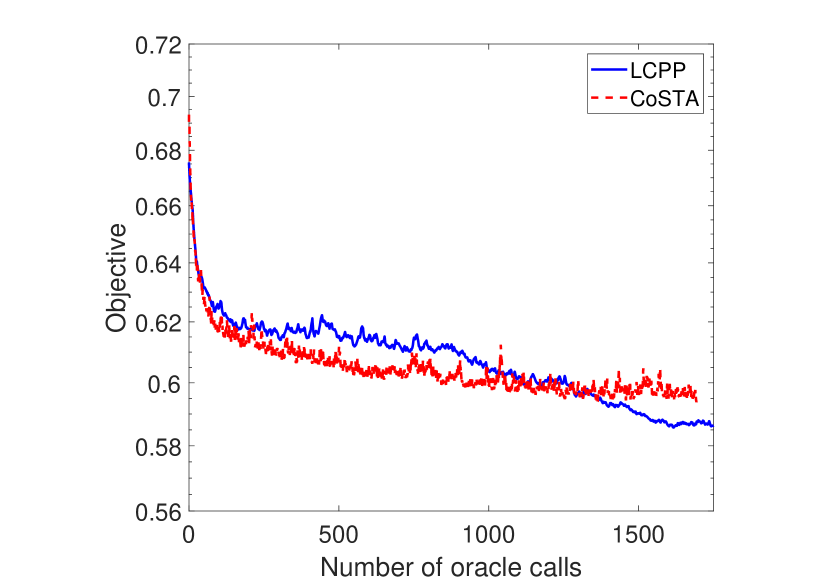
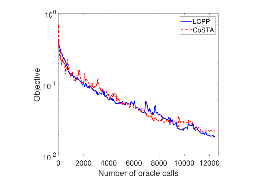
Refer to caption
(a) MNIST
Refer to caption
(b) gisette
Figure 2: Evolution of the objective function value across the number of calls to the oracle.
Refer to caption
Refer to caption
Refer to caption
Refer to caption
(a) Environment 1
Refer to caption
(b) Environment 2
Refer to caption
(c) Environment 3
Figure 3: Trajectory, energy, and mean constraint violation plots for N=60𝑁60N=60, T=15𝑇15T=15, and σ=0.2𝜎0.2\sigma=0.2, and environmental configurations 1, 2, and 3.
TABLE III: Classification accuracy of different algorithms for sparse logistic regression (where the entries are train accuracy/ test accuracy)
Dataset Accuracy LCPP CoSTA
MNIST train 90.5±1.4plus-or-minus90.51.490.5\pm 1.4 94±0.56plus-or-minus940.5694\pm 0.56
test 90.54±1.51plus-or-minus90.541.5190.54\pm 1.51 94.1±0.74plus-or-minus94.10.7494.1\pm 0.74
gisette train 99.7±.05plus-or-minus99.7.0599.7\pm.05 99.44±0.11plus-or-minus99.440.1199.44\pm 0.11
test 97.36±0.5plus-or-minus97.360.597.36\pm 0.5 97.72±0.32plus-or-minus97.720.3297.72\pm 0.32
Refer to caption
Refer to caption
Refer to caption
Refer to caption
(a) T=10𝑇10T=10
Refer to caption
(b) T=15𝑇15T=15
Refer to caption
(c) T=20𝑇20T=20
Figure 4: Trajectory, energy, and mean constraint violation plots for N=30𝑁30N=30, σ=0.2𝜎0.2\sigma=0.2, environmental configuration 4, and different values of T𝑇T.

V-B Energy-Optimal Trajectory Planning

Continuing the problem discussed in Sec. II, we apply CoSTA and CSSCA [13] to solve the energy-efficient trajectory planning problem (1)-(3) in a simulated 2D ocean environment. The ocean currents at a point 𝐱=[x1x2]𝖳𝐱superscriptdelimited-[]subscript𝑥1subscript𝑥2𝖳{\mathbf{x}}=[x_{1}~{}x_{2}]^{\mathsf{T}} are simulated using the following equations

ϑ(𝐱)=ω[12x122x1x2]exp{(x12+x22)}.italic-ϑ𝐱𝜔matrix12superscriptsubscript𝑥122subscript𝑥1subscript𝑥2superscriptsubscript𝑥12superscriptsubscript𝑥22\displaystyle\vartheta({\mathbf{x}})=\omega\begin{bmatrix}1-2x_{1}^{2}\\ -2x_{1}x_{2}\end{bmatrix}\exp\{-(x_{1}^{2}+x_{2}^{2})\}. (59)

We generate current predictions by adding biased noise as follows:

ϑ(𝐱,𝝃)=ϑ(𝐱)(𝐈+diag(𝐞(𝝃))),italic-ϑ𝐱𝝃italic-ϑ𝐱𝐈𝑑𝑖𝑎𝑔𝐞𝝃\displaystyle\vartheta({\mathbf{x}},{\boldsymbol{\xi}})=\vartheta({\mathbf{x}})(\mathbf{I}+diag(\mathbf{e}({\boldsymbol{\xi}}))), (60)

where 𝐞(𝝃)𝒩(𝟎,σ2𝐈)similar-to𝐞𝝃𝒩0superscript𝜎2𝐈\mathbf{e({\boldsymbol{\xi}})}\sim\mathcal{N}(\mathbf{0},\sigma^{2}\mathbf{I}). As stated earlier, neither the true ocean currents nor the noise model is known to the vehicle, which can only query the predictor for noisy realizations ϑ(𝐱,𝝃)italic-ϑ𝐱𝝃\vartheta({\mathbf{x}},{\boldsymbol{\xi}}) of the currents.

We carry out Monte Carlo simulations for multiple environments consisting of two agents and an obstacle. Each environment has a different starting, goal, and obstacle locations. Of these, the third environment, shown in Fig. 3(c) is particularly challenging, as the ocean currents tend to push one of the agents into the obstacle, requiring more precise navigation. We also vary the values of number of way points N𝑁N, mission time T𝑇T, and the noise parameter σ𝜎\sigma, so as to compare the performance of the proposed CoSTA algorithm with that of CSSCA across diverse settings.

The parameters of CSSCA (μ𝜇\mu, ρ𝜌\rho, and γ𝛾\gamma [13]) and CoSTA (μ𝜇\mu, k¯¯𝑘{\bar{k}}, c𝑐c, and w𝑤w) were tuned for best possible performance after running the algorithms for initial 100 iterations. The results are averaged over 10 Monte Carlo runs for the following values of problem parameters: ω=0.8𝜔0.8\omega=0.8, r0=0.7superscript𝑟00.7r^{0}=0.7m, r=0.1𝑟0.1r=0.1m, and vimax=1superscriptsubscript𝑣𝑖1v_{i}^{\max}=1m/s for i{1,2}𝑖12i\in\{1,2\}.

Fig. 3 shows the optimized trajectory of the agents along with energy and constraint violations for various environments and configurations. For each of the three environments depicted, both algorithms ultimately generate similar trajectories. However, CoSTA always converges faster, achieving the optimal energy and almost zero constraint violation in at most 30 iterations for environments 1 and 2. The convergence of both algorithms is slower on environment 3 as it is a more challenging one. For this environment CoSTA generates feasible trajectories for both the agents whereas CSSCA has non-zero constraint violation. These may be attributed to the adaptive step sizes in (11) of CoSTA unlike that of CSSCA, which allows our algorithm achieve a better progress towards an optimum.

Finally we plot trajectories and convergence plots for different mission times T𝑇T in Fig. 4. When the mission times are larger, both the algorithms generate longer paths so as to leverage the additional time and obtain trajectories with lower energy. On the other hand, it can be observed in Fig. 4 that for T=10𝑇10T=10, both the algorithms are unable to generate feasible trajectories within the stipulated 100 iterations. Hence, we conclude that higher mission times provide more flexibility to the algorithms so that they can generate feasible trajectories with zero constraint violation in fewer iterations. Finally, we observe the in all these cases, the proposed CoSTA algorithm converges faster than CSSCA.

VI Conclusion

We have considered the problem of minimizing a stochastic non-convex optimization problem with non-convex constraints. While the problem has been well-studied, the state-of-the-art algorithms have suboptimal oracle complexity of 𝒪(ϵ2)𝒪superscriptitalic-ϵ2{\mathcal{O}}(\epsilon^{-2}). We have proposed the CoSTA algorithm that introduces recursive momentum updates, thereby achieving the unimprovable oracle complexity of 𝒪(ϵ3/2)𝒪superscriptitalic-ϵ32{\mathcal{O}}(\epsilon^{-3/2}). The proposed algorithm is developed within the SCA framework, and requires convex surrogates of the objective and constraint functions at every iteration. We also introduced a parameterized version of the Mangasarian-Fromovitz constraint qualification that allows us to ensure that the intermediate subproblems are strictly feasible and the intermediate dual variable stay bounded, resulting in an oracle complexity bound that depends only on the problem parameters. Finally, the empirical performance of the proposed CoSTA algorithm is compared with the other state-of-the-art algorithms across two different applications: energy optimal trajectory design and sparse binary classification. The proposed algorithm outperforms the state-of-the-art algorithms on the energy optimal trajectory design problem and performs at par with the LCPP algorithm on the sparse binary classification problem.

Appendix A Proof of Lemma 1

Proof:

The proof follows along the lines of [31, Lemma 2]. Expanding 𝐳t+1U(𝐱t)subscript𝐳𝑡1𝑈subscript𝐱𝑡{\mathbf{z}}_{t+1}-\nabla U({\mathbf{x}}_{t}) from (7) and introducing (1βt+1)U(𝐱t)1subscript𝛽𝑡1𝑈subscript𝐱𝑡(1-\beta_{t+1})\nabla U({\mathbf{x}}_{t}), we obtain

𝐳t+2U(𝐱t+1)=subscript𝐳𝑡2𝑈subscript𝐱𝑡1absent\displaystyle{\mathbf{z}}_{t+2}-\nabla U({\mathbf{x}}_{t+1})= (1βt+1)(𝐳t+1U(𝐱t))(1βt+1)(f(𝐱t,𝝃t+1)U(𝐱t))1subscript𝛽𝑡1subscript𝐳𝑡1𝑈subscript𝐱𝑡1subscript𝛽𝑡1𝑓subscript𝐱𝑡subscript𝝃𝑡1𝑈subscript𝐱𝑡\displaystyle(1-\beta_{t+1})({\mathbf{z}}_{t+1}-\nabla U({\mathbf{x}}_{t}))-(1-\beta_{t+1})(\nabla f({\mathbf{x}}_{t},{\boldsymbol{\xi}}_{t+1})-\nabla U({\mathbf{x}}_{t}))
+f(𝐱t+1,𝝃t+1)U(𝐱t+1)𝑓subscript𝐱𝑡1subscript𝝃𝑡1𝑈subscript𝐱𝑡1\displaystyle+\nabla f({\mathbf{x}}_{t+1},{\boldsymbol{\xi}}_{t+1})-\nabla U({\mathbf{x}}_{t+1}) (61)

where observe that 𝔼𝝃t[U(𝐱t)f(𝐱t,𝝃t+1)]=𝔼𝝃t[f(𝐱t+1,𝝃t+1)U(𝐱t+1)]=0subscript𝔼subscript𝝃𝑡delimited-[]𝑈subscript𝐱𝑡𝑓subscript𝐱𝑡subscript𝝃𝑡1subscript𝔼subscript𝝃𝑡delimited-[]𝑓subscript𝐱𝑡1subscript𝝃𝑡1𝑈subscript𝐱𝑡10{\mathbb{E}}_{{\boldsymbol{\xi}}_{t}}[\nabla U({\mathbf{x}}_{t})-\nabla f({\mathbf{x}}_{t},{\boldsymbol{\xi}}_{t+1})]={\mathbb{E}}_{{\boldsymbol{\xi}}_{t}}[\nabla f({\mathbf{x}}_{t+1},{\boldsymbol{\xi}}_{t+1})-\nabla U({\mathbf{x}}_{t+1})]=0. Therefore, we have that

𝔼𝝃t+1[𝐳t+2U(𝐱t+1)2ηt(12βt+1)]=𝔼𝝃t+1[(1βt+1)2𝐳t+1U(𝐱t)2ηt(12βt+1)]subscript𝔼subscript𝝃𝑡1delimited-[]superscriptnormsubscript𝐳𝑡2𝑈subscript𝐱𝑡12subscript𝜂𝑡12subscript𝛽𝑡1subscript𝔼subscript𝝃𝑡1delimited-[]superscript1subscript𝛽𝑡12superscriptnormsubscript𝐳𝑡1𝑈subscript𝐱𝑡2subscript𝜂𝑡12subscript𝛽𝑡1\displaystyle{\mathbb{E}}_{{\boldsymbol{\xi}}_{t+1}}\bigg{[}\frac{\left\|{\mathbf{z}}_{t+2}-\nabla U({\mathbf{x}}_{t+1})\right\|^{2}}{\eta_{t}(1-2\beta_{t+1})}\bigg{]}~{}={\mathbb{E}}_{{\boldsymbol{\xi}}_{t+1}}\bigg{[}\frac{(1-\beta_{t+1})^{2}\left\|{\mathbf{z}}_{t+1}-\nabla U({\mathbf{x}}_{t})\right\|^{2}}{\eta_{t}(1-2\beta_{t+1})}\bigg{]}
+𝔼𝝃t+1[ηt1(12βt+1)1(1βt+1)(f(𝐱t,𝝃t+1)\displaystyle~{}+{\mathbb{E}}_{{\boldsymbol{\xi}}_{t+1}}\Big{[}\eta_{t}^{-1}(1-2\beta_{t+1})^{-1}\big{\|}(1-\beta_{t+1})\big{(}\nabla f({\mathbf{x}}_{t},{\boldsymbol{\xi}}_{t+1})
U(𝐱t)+U(𝐱t+1)f(𝐱t+1,𝝃t+1))+βt+1(f(𝐱t+1,𝝃t+1)U(𝐱t+1)))2]\displaystyle~{}~{}~{}-\nabla U({\mathbf{x}}_{t})+\nabla U({\mathbf{x}}_{t+1})-\nabla f({\mathbf{x}}_{t+1},{\boldsymbol{\xi}}_{t+1})\big{)}+\beta_{t+1}\big{(}\nabla f({\mathbf{x}}_{t+1},{\boldsymbol{\xi}}_{t+1})-\nabla U({\mathbf{x}}_{t+1}))\big{)}\big{\|}^{2}\Big{]} (62)

where the cross term vanishes since 𝐳t+1U(𝐱t)subscript𝐳𝑡1𝑈subscript𝐱𝑡{\mathbf{z}}_{t+1}-\nabla U({\mathbf{x}}_{t}) is independent of 𝝃t+1subscript𝝃𝑡1{\boldsymbol{\xi}}_{t+1} and the second summand is zero mean. The second term in (62) can again be expanded as

𝔼𝝃t+1[ηt1(12βt+1)1(1βt+1)(f(𝐱t,𝝃t+1)\displaystyle{\mathbb{E}}_{{\boldsymbol{\xi}}_{t+1}}\Big{[}\eta_{t}^{-1}(1-2\beta_{t+1})^{-1}\big{\|}(1-\beta_{t+1})\big{(}\nabla f({\mathbf{x}}_{t},{\boldsymbol{\xi}}_{t+1})
U(𝐱t)+U(𝐱t+1)f(𝐱t+1,𝝃t+1))\displaystyle~{}~{}~{}~{}~{}-\nabla U({\mathbf{x}}_{t})+\nabla U({\mathbf{x}}_{t+1})-\nabla f({\mathbf{x}}_{t+1},{\boldsymbol{\xi}}_{t+1})\big{)}
+βt+1(f(𝐱t+1,𝝃t+1)U(𝐱t+1)))2]\displaystyle~{}~{}~{}~{}~{}~{}~{}~{}~{}~{}~{}+\beta_{t+1}\big{(}\nabla f({\mathbf{x}}_{t+1},{\boldsymbol{\xi}}_{t+1})-\nabla U({\mathbf{x}}_{t+1}))\big{)}\big{\|}^{2}\Big{]}
(a)2𝔼𝝃t+1[(1βt+1)2f(𝐱t+1,𝝃t+1)f(𝐱t,𝝃t+1)2ηt(12βt+1)]𝑎2subscript𝔼subscript𝝃𝑡1delimited-[]superscript1subscript𝛽𝑡12superscriptnorm𝑓subscript𝐱𝑡1subscript𝝃𝑡1𝑓subscript𝐱𝑡subscript𝝃𝑡12subscript𝜂𝑡12subscript𝛽𝑡1\displaystyle\overset{(a)}{\leq}2{\mathbb{E}}_{{\boldsymbol{\xi}}_{t+1}}\bigg{[}\frac{(1-\beta_{t+1})^{2}\left\|\nabla f({\mathbf{x}}_{t+1},{\boldsymbol{\xi}}_{t+1})-\nabla f({\mathbf{x}}_{t},{\boldsymbol{\xi}}_{t+1})\right\|^{2}}{\eta_{t}(1-2\beta_{t+1})}\bigg{]}
+2𝔼𝝃t+1[βt+12f(𝐱t+1,𝝃t+1)U(𝐱t+1)2ηt(12βt+1)]2subscript𝔼subscript𝝃𝑡1delimited-[]superscriptsubscript𝛽𝑡12superscriptnorm𝑓subscript𝐱𝑡1subscript𝝃𝑡1𝑈subscript𝐱𝑡12subscript𝜂𝑡12subscript𝛽𝑡1\displaystyle~{}~{}~{}~{}~{}~{}~{}~{}~{}~{}+2{\mathbb{E}}_{{\boldsymbol{\xi}}_{t+1}}\bigg{[}\frac{\beta_{t+1}^{2}\left\|\nabla f({\mathbf{x}}_{t+1},{\boldsymbol{\xi}}_{t+1})-\nabla U({\mathbf{x}}_{t+1})\right\|^{2}}{\eta_{t}(1-2\beta_{t+1})}\bigg{]}
(b)2𝔼𝝃t+1[(1βt+1)2f(𝐱t+1,𝝃t+1)f(𝐱t,𝝃t+1)2ηt(12βt+1)]𝑏2subscript𝔼subscript𝝃𝑡1delimited-[]superscript1subscript𝛽𝑡12superscriptnorm𝑓subscript𝐱𝑡1subscript𝝃𝑡1𝑓subscript𝐱𝑡subscript𝝃𝑡12subscript𝜂𝑡12subscript𝛽𝑡1\displaystyle\overset{(b)}{\leq}2{\mathbb{E}}_{{\boldsymbol{\xi}}_{t+1}}\bigg{[}\frac{(1-\beta_{t+1})^{2}\left\|\nabla f({\mathbf{x}}_{t+1},{\boldsymbol{\xi}}_{t+1})-\nabla f({\mathbf{x}}_{t},{\boldsymbol{\xi}}_{t+1})\right\|^{2}}{\eta_{t}(1-2\beta_{t+1})}\bigg{]}
+2𝔼𝝃t+1[βt+12f(𝐱t+1,𝝃t+1)2ηt(12βt+1)]2subscript𝔼subscript𝝃𝑡1delimited-[]superscriptsubscript𝛽𝑡12superscriptnorm𝑓subscript𝐱𝑡1subscript𝝃𝑡12subscript𝜂𝑡12subscript𝛽𝑡1\displaystyle~{}~{}~{}~{}~{}~{}~{}~{}~{}~{}+2{\mathbb{E}}_{{\boldsymbol{\xi}}_{t+1}}\bigg{[}\frac{\beta_{t+1}^{2}\left\|\nabla f({\mathbf{x}}_{t+1},{\boldsymbol{\xi}}_{t+1})\right\|^{2}}{\eta_{t}(1-2\beta_{t+1})}\bigg{]} (63)

where in (a) we have used the inequality 𝔼[𝖷𝔼[𝖷]+𝖸2]2𝔼[𝖷2]+2𝔼[𝖸2]𝔼delimited-[]superscriptnorm𝖷𝔼delimited-[]𝖷𝖸22𝔼delimited-[]superscriptnorm𝖷22𝔼delimited-[]superscriptnorm𝖸2{\mathbb{E}}[\left\|\mathsf{X}-{\mathbb{E}}[\mathsf{X}]+\mathsf{Y}\right\|^{2}]\leq 2{\mathbb{E}}[\left\|\mathsf{X}\right\|^{2}]+2{\mathbb{E}}[\left\|\mathsf{Y}\right\|^{2}] for any random variables 𝖷𝖷\mathsf{X} and 𝖸𝖸\mathsf{Y} with bounded variances. And in (b) we have used 𝔼[𝖷𝔼[𝖷]2]𝔼[𝖷2]𝔼delimited-[]superscriptnorm𝖷𝔼delimited-[]𝖷2𝔼delimited-[]superscriptnorm𝖷2{\mathbb{E}}[\left\|\mathsf{X}-{\mathbb{E}}\left[\mathsf{X}\right]\right\|^{2}]\leq{\mathbb{E}}[\left\|\mathsf{X}\right\|^{2}]. Dividing both sides by 116L2116superscript𝐿2\tfrac{1}{16L^{2}}, taking full expectation in (62) and using βt+11subscript𝛽𝑡11\beta_{t+1}\leq 1 (23) can be rewritten as,

116L2𝔼[𝜺t+12ηt(12βt+1)]116superscript𝐿2𝔼delimited-[]superscriptnormsubscript𝜺𝑡12subscript𝜂𝑡12subscript𝛽𝑡1absent\displaystyle\frac{1}{16L^{2}}{\mathbb{E}}\left[\frac{\left\|{{\boldsymbol{\varepsilon}}}_{t+1}\right\|^{2}}{\eta_{t}(1-2\beta_{t+1})}\right]\leq 116L2𝔼[𝜺t2ηt]+18L2𝔼[f(𝐱t+1,𝝃t+1)f(𝐱t,𝝃t+1)2ηt]116superscript𝐿2𝔼delimited-[]superscriptnormsubscript𝜺𝑡2subscript𝜂𝑡18superscript𝐿2𝔼delimited-[]superscriptnorm𝑓subscript𝐱𝑡1subscript𝝃𝑡1𝑓subscript𝐱𝑡subscript𝝃𝑡12subscript𝜂𝑡\displaystyle\frac{1}{16L^{2}}{\mathbb{E}}\left[\frac{\left\|{{\boldsymbol{\varepsilon}}}_{t}\right\|^{2}}{\eta_{t}}\right]+\frac{1}{8L^{2}}{\mathbb{E}}\left[\frac{\left\|\nabla f({\mathbf{x}}_{t+1},{\boldsymbol{\xi}}_{t+1})-\nabla f({\mathbf{x}}_{t},{\boldsymbol{\xi}}_{t+1})\right\|^{2}}{\eta_{t}}\right]
+18L2𝔼[βt+12Gt+12ηt(12βt+1)]18superscript𝐿2𝔼delimited-[]superscriptsubscript𝛽𝑡12superscriptsubscript𝐺𝑡12subscript𝜂𝑡12subscript𝛽𝑡1\displaystyle~{}~{}~{}~{}+\frac{1}{8L^{2}}{\mathbb{E}}\left[\frac{\beta_{t+1}^{2}G_{t+1}^{2}}{\eta_{t}(1-2\beta_{t+1})}\right] (64)

Using L𝐿L-smoothness, and the update equation (10), we obtain

116L2𝔼[𝜺t+12ηt(12βt+1)]116superscript𝐿2𝔼delimited-[]superscriptnormsubscript𝜺𝑡12subscript𝜂𝑡12subscript𝛽𝑡1\displaystyle\frac{1}{16L^{2}}{\mathbb{E}}\left[\frac{\left\|{{\boldsymbol{\varepsilon}}}_{t+1}\right\|^{2}}{\eta_{t}(1-2\beta_{t+1})}\right] 116L2𝔼[𝜺t2ηt]+18𝔼[𝐱t+1𝐱t2ηt]+18L2𝔼[βt+12Gt+12ηt(12βt+1)]absent116superscript𝐿2𝔼delimited-[]superscriptnormsubscript𝜺𝑡2subscript𝜂𝑡18𝔼delimited-[]superscriptnormsubscript𝐱𝑡1subscript𝐱𝑡2subscript𝜂𝑡18superscript𝐿2𝔼delimited-[]superscriptsubscript𝛽𝑡12superscriptsubscript𝐺𝑡12subscript𝜂𝑡12subscript𝛽𝑡1\displaystyle\leq\frac{1}{16L^{2}}{\mathbb{E}}\left[\frac{\left\|{{\boldsymbol{\varepsilon}}}_{t}\right\|^{2}}{\eta_{t}}\right]+\frac{1}{8}{\mathbb{E}}\left[\frac{\left\|{\mathbf{x}}_{t+1}-{\mathbf{x}}_{t}\right\|^{2}}{\eta_{t}}\right]+\frac{1}{8L^{2}}{\mathbb{E}}\left[\frac{\beta_{t+1}^{2}G_{t+1}^{2}}{\eta_{t}(1-2\beta_{t+1})}\right]
116L2𝔼[𝜺t2ηt]+18𝔼[ηt𝜹t2]+18L2𝔼[βt+12Gt+12ηt(12βt+1)].absent116superscript𝐿2𝔼delimited-[]superscriptnormsubscript𝜺𝑡2subscript𝜂𝑡18𝔼delimited-[]subscript𝜂𝑡superscriptnormsubscript𝜹𝑡218superscript𝐿2𝔼delimited-[]superscriptsubscript𝛽𝑡12superscriptsubscript𝐺𝑡12subscript𝜂𝑡12subscript𝛽𝑡1\displaystyle\leq\frac{1}{16L^{2}}{\mathbb{E}}\left[\frac{\left\|{{\boldsymbol{\varepsilon}}}_{t}\right\|^{2}}{\eta_{t}}\right]+\frac{1}{8}{\mathbb{E}}\left[\eta_{t}\left\|{\boldsymbol{\delta}}_{t}\right\|^{2}\right]+\frac{1}{8L^{2}}{\mathbb{E}}\left[\frac{\beta_{t+1}^{2}G_{t+1}^{2}}{\eta_{t}(1-2\beta_{t+1})}\right]. (65)

Appendix B Proof of Lemma 2

Proof:

We first obtain a fundamental inequality. The optimality condition of (𝒫tsubscript𝒫𝑡\mathcal{P}_{t}) implies that

𝐲𝐱^t,f~(𝐱^t,𝐱t,𝐳t,𝝃t)+𝐯𝐱^t0𝐲subscript^𝐱𝑡~𝑓subscript^𝐱𝑡subscript𝐱𝑡subscript𝐳𝑡subscript𝝃𝑡subscript𝐯subscript^𝐱𝑡0\displaystyle\big{\langle}{\mathbf{y}}-{{\hat{{\mathbf{x}}}}_{t}},\nabla{\tilde{f}}({{\hat{{\mathbf{x}}}}_{t}},{\mathbf{x}}_{t},{\mathbf{z}}_{t},{\boldsymbol{\xi}}_{t})+{\mathbf{v}}_{{\hat{{\mathbf{x}}}}_{t}}\big{\rangle}\geq 0 (66)

for all 𝐲𝒳(𝐱t)𝐲𝒳subscript𝐱𝑡{\mathbf{y}}\in{\mathcal{X}}({\mathbf{x}}_{t}), where 𝐯𝐱^tu(𝐱^t)subscript𝐯subscript^𝐱𝑡𝑢subscript^𝐱𝑡{\mathbf{v}}_{{\hat{{\mathbf{x}}}}_{t}}\in\partial u({{\hat{{\mathbf{x}}}}_{t}}). Choosing 𝐲=𝐱t𝐲subscript𝐱𝑡{\mathbf{y}}={\mathbf{x}}_{t},

𝐱t𝐱^t,f~(𝐱^t,𝐱t,𝐳t,𝝃t)+𝐯𝐱^t0.subscript𝐱𝑡subscript^𝐱𝑡~𝑓subscript^𝐱𝑡subscript𝐱𝑡subscript𝐳𝑡subscript𝝃𝑡subscript𝐯subscript^𝐱𝑡0\displaystyle\big{\langle}{\mathbf{x}}_{t}-{{\hat{{\mathbf{x}}}}_{t}},\nabla{\tilde{f}}({{\hat{{\mathbf{x}}}}_{t}},{\mathbf{x}}_{t},{\mathbf{z}}_{t},{\boldsymbol{\xi}}_{t})+{\mathbf{v}}_{{\hat{{\mathbf{x}}}}_{t}}\big{\rangle}\geq 0. (67)

Adding and subtracting f~(𝐱t,𝐱t,𝐳t,𝝃t)=𝐳t+1~𝑓subscript𝐱𝑡subscript𝐱𝑡subscript𝐳𝑡subscript𝝃𝑡subscript𝐳𝑡1\nabla{\tilde{f}}({\mathbf{x}}_{t},{\mathbf{x}}_{t},{\mathbf{z}}_{t},{\boldsymbol{\xi}}_{t})={\mathbf{z}}_{t+1}, we obtain

𝐱^t𝐱t,𝐳t+1+𝐯𝐱^t+𝐱^t𝐱t,f~(𝐱^t,𝐱t,𝐳t,𝝃t)f~(𝐱t,𝐱t,𝐳t,𝝃t)0.subscript^𝐱𝑡subscript𝐱𝑡subscript𝐳𝑡1subscript𝐯subscript^𝐱𝑡subscript^𝐱𝑡subscript𝐱𝑡~𝑓subscript^𝐱𝑡subscript𝐱𝑡subscript𝐳𝑡subscript𝝃𝑡~𝑓subscript𝐱𝑡subscript𝐱𝑡subscript𝐳𝑡subscript𝝃𝑡0\displaystyle\langle{{\hat{{\mathbf{x}}}}_{t}}-{\mathbf{x}}_{t},{\mathbf{z}}_{t+1}+{\mathbf{v}}_{{\hat{{\mathbf{x}}}}_{t}}\rangle+\langle{{\hat{{\mathbf{x}}}}_{t}}-{\mathbf{x}}_{t},\nabla{\tilde{f}}({{\hat{{\mathbf{x}}}}_{t}},{\mathbf{x}}_{t},{\mathbf{z}}_{t},{\boldsymbol{\xi}}_{t})-\nabla{\tilde{f}}({\mathbf{x}}_{t},{\mathbf{x}}_{t},{\mathbf{z}}_{t},{\boldsymbol{\xi}}_{t})\rangle\leq 0. (68)
𝐳t+1+𝐯𝐱^t,𝐱^t𝐱t+μ𝐱^t𝐱t20.absentsubscript𝐳𝑡1subscript𝐯subscript^𝐱𝑡subscript^𝐱𝑡subscript𝐱𝑡𝜇superscriptnormsubscript^𝐱𝑡subscript𝐱𝑡20\displaystyle\Rightarrow\langle{\mathbf{z}}_{t+1}+{\mathbf{v}}_{{\hat{{\mathbf{x}}}}_{t}},{{\hat{{\mathbf{x}}}}_{t}}-{\mathbf{x}}_{t}\rangle+\mu\left\|{{\hat{{\mathbf{x}}}}_{t}}-{\mathbf{x}}_{t}\right\|^{2}\leq 0. (69)

where we have used the strong monotonicity property of the gradient of the strongly convex function f~(,𝐱t,𝐳t,𝝃t)~𝑓subscript𝐱𝑡subscript𝐳𝑡subscript𝝃𝑡{\tilde{f}}(\cdot,{\mathbf{x}}_{t},{\mathbf{z}}_{t},{\boldsymbol{\xi}}_{t}). From the convexity of u𝑢u and the update rule (10), we obtain

u(𝐱t+1)u(𝐱t)𝑢subscript𝐱𝑡1𝑢subscript𝐱𝑡\displaystyle u{({\mathbf{x}}_{t+1})}-u({\mathbf{x}}_{t}) ηt𝐯𝐱^t,𝐱^t𝐱tabsentsubscript𝜂𝑡subscript𝐯subscript^𝐱𝑡subscript^𝐱𝑡subscript𝐱𝑡\displaystyle\leq\eta_{t}\langle{\mathbf{v}}_{{\hat{{\mathbf{x}}}}_{t}},{{\hat{{\mathbf{x}}}}_{t}}-{\mathbf{x}}_{t}\rangle (70)

Multiplying (69) by ηtsubscript𝜂𝑡\eta_{t} and adding, we obtain

ηt𝐳t+1,𝐱^t𝐱tμηt𝐱^t𝐱t2+u(𝐱t)u(𝐱t+1).subscript𝜂𝑡subscript𝐳𝑡1subscript^𝐱𝑡subscript𝐱𝑡𝜇subscript𝜂𝑡superscriptnormsubscript^𝐱𝑡subscript𝐱𝑡2𝑢subscript𝐱𝑡𝑢subscript𝐱𝑡1\displaystyle\eta_{t}\langle{\mathbf{z}}_{t+1},{{\hat{{\mathbf{x}}}}_{t}}-{\mathbf{x}}_{t}\rangle\leq-\mu\eta_{t}\left\|{{\hat{{\mathbf{x}}}}_{t}}-{\mathbf{x}}_{t}\right\|^{2}+u({\mathbf{x}}_{t})-u({\mathbf{x}}_{t+1}). (71)

Adding and subtracting U(𝐱t)𝑈subscript𝐱𝑡\nabla U({\mathbf{x}}_{t}), we obtain

ηt𝐳t+1U(𝐱t),𝐱^t𝐱t+ηtU(𝐱t),𝐱^t𝐱tsubscript𝜂𝑡subscript𝐳𝑡1𝑈subscript𝐱𝑡subscript^𝐱𝑡subscript𝐱𝑡subscript𝜂𝑡𝑈subscript𝐱𝑡subscript^𝐱𝑡subscript𝐱𝑡\displaystyle\eta_{t}\langle{\mathbf{z}}_{t+1}-\nabla U({\mathbf{x}}_{t}),{{\hat{{\mathbf{x}}}}_{t}}-{\mathbf{x}}_{t}\rangle+\eta_{t}\langle\nabla U({\mathbf{x}}_{t}),{{\hat{{\mathbf{x}}}}_{t}}-{\mathbf{x}}_{t}\rangle
μηt𝐱^t𝐱t2+u(𝐱t)u(𝐱t+1)absent𝜇subscript𝜂𝑡superscriptnormsubscript^𝐱𝑡subscript𝐱𝑡2𝑢subscript𝐱𝑡𝑢subscript𝐱𝑡1\displaystyle~{}~{}~{}\leq-\mu\eta_{t}\left\|{{\hat{{\mathbf{x}}}}_{t}}-{\mathbf{x}}_{t}\right\|^{2}+u({\mathbf{x}}_{t})-u({\mathbf{x}}_{t+1}) (72)

We now proceed to bound U(𝐱t+1)𝑈subscript𝐱𝑡1U({\mathbf{x}}_{t+1}) in terms of U(𝐱t)𝑈subscript𝐱𝑡U({\mathbf{x}}_{t}). Since U𝑈U is smooth, we have that:

U(𝐱t+1)U(𝐱t)+U(𝐱t),𝐱t+1𝐱t+L2𝐱t+1𝐱t2𝑈subscript𝐱𝑡1𝑈subscript𝐱𝑡𝑈subscript𝐱𝑡subscript𝐱𝑡1subscript𝐱𝑡𝐿2superscriptnormsubscript𝐱𝑡1subscript𝐱𝑡2\displaystyle U({\mathbf{x}}_{t+1})\leq U({\mathbf{x}}_{t})+\langle\nabla U({\mathbf{x}}_{t}),{\mathbf{x}}_{t+1}-{\mathbf{x}}_{t}\rangle+\frac{L}{2}\left\|{\mathbf{x}}_{t+1}-{\mathbf{x}}_{t}\right\|^{2} (73)
U(𝐱t)+ηtU(𝐱t),𝐱^t𝐱t+Lηt22𝐱^t𝐱t2absent𝑈subscript𝐱𝑡subscript𝜂𝑡𝑈subscript𝐱𝑡subscript^𝐱𝑡subscript𝐱𝑡𝐿superscriptsubscript𝜂𝑡22superscriptnormsubscript^𝐱𝑡subscript𝐱𝑡2\displaystyle\leq U({\mathbf{x}}_{t})+\eta_{t}\langle\nabla U({\mathbf{x}}_{t}),{{\hat{{\mathbf{x}}}}_{t}}-{\mathbf{x}}_{t}\rangle+\frac{L\eta_{t}^{2}}{2}\left\|{{\hat{{\mathbf{x}}}}_{t}}-{\mathbf{x}}_{t}\right\|^{2} (74)
U(𝐱t)+u(𝐱t)u(𝐱t+1)ηt𝐳t+1U(𝐱t),𝐱^t𝐱t+(L2ηt2μηt)𝐱^t𝐱t2absent𝑈subscript𝐱𝑡𝑢subscript𝐱𝑡𝑢subscript𝐱𝑡1subscript𝜂𝑡subscript𝐳𝑡1𝑈subscript𝐱𝑡subscript^𝐱𝑡subscript𝐱𝑡𝐿2superscriptsubscript𝜂𝑡2𝜇subscript𝜂𝑡superscriptnormsubscript^𝐱𝑡subscript𝐱𝑡2\displaystyle\leq U({\mathbf{x}}_{t})+u({\mathbf{x}}_{t})-u({\mathbf{x}}_{t+1})-\eta_{t}\langle{\mathbf{z}}_{t+1}-\nabla U({\mathbf{x}}_{t}),{{\hat{{\mathbf{x}}}}_{t}}-{\mathbf{x}}_{t}\rangle+\bigg{(}\frac{L}{2}\eta_{t}^{2}-\mu\eta_{t}\bigg{)}\left\|{{\hat{{\mathbf{x}}}}_{t}}-{\mathbf{x}}_{t}\right\|^{2} (75)

where the last inequality follows from substituting (72). Using Young’s inequality, rearranging, and taking expectation on both sides, we obtain

𝔼[F(𝐱t+1)F(𝐱t)]𝔼delimited-[]𝐹subscript𝐱𝑡1𝐹subscript𝐱𝑡\displaystyle{\mathbb{E}}\left[F({\mathbf{x}}_{t+1})-F({\mathbf{x}}_{t})\right] 12𝔼[ηtU(𝐱t)𝐳t+12]absent12𝔼delimited-[]subscript𝜂𝑡superscriptnorm𝑈subscript𝐱𝑡subscript𝐳𝑡12\displaystyle\leq\frac{1}{2}{\mathbb{E}}\left[\eta_{t}\left\|\nabla U({\mathbf{x}}_{t})-{\mathbf{z}}_{t+1}\right\|^{2}\right]
+L2𝔼[ηt2𝐱^t𝐱t2]+(12μ)ηt𝔼[𝐱^t𝐱t2]𝐿2𝔼delimited-[]superscriptsubscript𝜂𝑡2superscriptnormsubscript^𝐱𝑡subscript𝐱𝑡212𝜇subscript𝜂𝑡𝔼delimited-[]superscriptnormsubscript^𝐱𝑡subscript𝐱𝑡2\displaystyle~{}~{}~{}+\frac{L}{2}{\mathbb{E}}\left[\eta_{t}^{2}\left\|{{\hat{{\mathbf{x}}}}_{t}}-{\mathbf{x}}_{t}\right\|^{2}\right]+\bigg{(}\frac{1}{2}-\mu\bigg{)}\eta_{t}{\mathbb{E}}\left[\left\|{{\hat{{\mathbf{x}}}}_{t}}-{\mathbf{x}}_{t}\right\|^{2}\right]
12𝔼[ηt𝜺t2]14𝔼[(4μ2Lηt2)ηt𝜹t2]absent12𝔼delimited-[]subscript𝜂𝑡superscriptnormsubscript𝜺𝑡214𝔼delimited-[]4𝜇2𝐿subscript𝜂𝑡2subscript𝜂𝑡superscriptnormsubscript𝜹𝑡2\displaystyle\leq\frac{1}{2}{\mathbb{E}}\left[\eta_{t}\left\|{{\boldsymbol{\varepsilon}}}_{t}\right\|^{2}\right]-\frac{1}{4}{\mathbb{E}}\left[(4\mu-2L\eta_{t}-2)\eta_{t}\left\|{\boldsymbol{\delta}}_{t}\right\|^{2}\right] (76)

Finally, using μ>Lηt2+34𝜇𝐿subscript𝜂𝑡234\mu>\frac{L\eta_{t}}{2}+\frac{3}{4}, we get the desired result. ∎

Appendix C Proof of Lemma 4

Proof:

Since 𝐱t𝒳subscript𝐱𝑡𝒳{\mathbf{x}}_{t}\in{\mathcal{X}}, strong MFCQ holds at 𝐱tsubscript𝐱𝑡{\mathbf{x}}_{t}, implying the existence of 𝐝tsubscript𝐝𝑡{\mathbf{d}}_{t} as specified in Assumption (A5). Consider the point 𝐱~(𝐱t)=𝐱t+γ𝐝t~𝐱subscript𝐱𝑡subscript𝐱𝑡𝛾subscript𝐝𝑡{\tilde{\mathbf{x}}}({\mathbf{x}}_{t})={\mathbf{x}}_{t}+\gamma{\mathbf{d}}_{t} for γ>0𝛾0\gamma>0 and let ¯¯{\bar{\mathcal{I}}} and 𝒥¯¯𝒥{\bar{\mathcal{J}}} be defined as the sets of indices corresponding to the near-active constraints at 𝐱tsubscript𝐱𝑡{\mathbf{x}}_{t} for the convex and general constraints, respectively.

First consider the near-active constraints at the feasible point 𝐱tsubscript𝐱𝑡{\mathbf{x}}_{t}. From the smoothness of g~j(,𝐱t)subscript~𝑔𝑗subscript𝐱𝑡{\tilde{g}}_{j}(\cdot,{\mathbf{x}}_{t}), we have that

g~j(𝐱~(𝐱t),𝐱t)subscript~𝑔𝑗~𝐱subscript𝐱𝑡subscript𝐱𝑡\displaystyle{\tilde{g}}_{j}({\tilde{\mathbf{x}}}({\mathbf{x}}_{t}),{\mathbf{x}}_{t}) g~j(𝐱t,𝐱t)+g~j(𝐱t,𝐱t),𝐱~(𝐱t)𝐱t+L2𝐱~(𝐱t)𝐱t2absentsubscript~𝑔𝑗subscript𝐱𝑡subscript𝐱𝑡subscript~𝑔𝑗subscript𝐱𝑡subscript𝐱𝑡~𝐱subscript𝐱𝑡subscript𝐱𝑡𝐿2superscriptnorm~𝐱subscript𝐱𝑡subscript𝐱𝑡2\displaystyle\leq{\tilde{g}}_{j}({\mathbf{x}}_{t},{\mathbf{x}}_{t})+\langle\nabla{\tilde{g}}_{j}({\mathbf{x}}_{t},{\mathbf{x}}_{t}),{\tilde{\mathbf{x}}}({\mathbf{x}}_{t})-{\mathbf{x}}_{t}\rangle+\frac{L}{2}\left\|{\tilde{\mathbf{x}}}({\mathbf{x}}_{t})-{\mathbf{x}}_{t}\right\|^{2} (77)
=g~j(𝐱t)+γg~j(𝐱t),𝐝t+γ2L2ργ+γ2L2absentsubscript~𝑔𝑗subscript𝐱𝑡𝛾subscript~𝑔𝑗subscript𝐱𝑡subscript𝐝𝑡superscript𝛾2𝐿2𝜌𝛾superscript𝛾2𝐿2\displaystyle={\tilde{g}}_{j}({\mathbf{x}}_{t})+\gamma\langle\nabla{\tilde{g}}_{j}({\mathbf{x}}_{t}),{\mathbf{d}}_{t}\rangle+\frac{\gamma^{2}L}{2}\leq-\rho\gamma+\frac{\gamma^{2}L}{2} (78)

for all j𝒥¯𝑗¯𝒥j\in{\bar{\mathcal{J}}}. Likewise, from the smoothness of hisubscript𝑖h_{i}, we have that

hi(𝐱~(𝐱t))subscript𝑖~𝐱subscript𝐱𝑡\displaystyle h_{i}({\tilde{\mathbf{x}}}({\mathbf{x}}_{t})) ργ+γ2L2absent𝜌𝛾superscript𝛾2𝐿2\displaystyle\leq-\rho\gamma+\frac{\gamma^{2}L}{2} (79)

for all i¯𝑖¯i\in{\bar{\mathcal{I}}}. Therefore, if we set γ=ρL𝛾𝜌𝐿\gamma=\frac{\rho}{L}, it can be seen that g~j(𝐱~(𝐱t),𝐱t)ρ22Lsubscript~𝑔𝑗~𝐱subscript𝐱𝑡subscript𝐱𝑡superscript𝜌22𝐿{\tilde{g}}_{j}({\tilde{\mathbf{x}}}({\mathbf{x}}_{t}),{\mathbf{x}}_{t})\leq-\frac{\rho^{2}}{2L} and hi(𝐱~(𝐱t))ρ22Lsubscript𝑖~𝐱subscript𝐱𝑡superscript𝜌22𝐿h_{i}({\tilde{\mathbf{x}}}({\mathbf{x}}_{t}))\leq-\frac{\rho^{2}}{2L} as required. Since 𝐱~(𝐱t)𝒳~𝐱subscript𝐱𝑡𝒳{\tilde{\mathbf{x}}}({\mathbf{x}}_{t})\in{\mathcal{X}}, it follows from Assumption A1 that 𝐱~(𝐱t)𝒟~𝐱subscript𝐱𝑡𝒟{\tilde{\mathbf{x}}}({\mathbf{x}}_{t})\in{\mathcal{D}} and both the constraint functions are well-defined at 𝐱~(𝐱t)~𝐱subscript𝐱𝑡{\tilde{\mathbf{x}}}({\mathbf{x}}_{t}).

Next, let us consider the strongly inactive constraints, where we have that

g~j(𝐱~(𝐱t),𝐱t)subscript~𝑔𝑗~𝐱subscript𝐱𝑡subscript𝐱𝑡\displaystyle{\tilde{g}}_{j}({\tilde{\mathbf{x}}}({\mathbf{x}}_{t}),{\mathbf{x}}_{t}) =g~j(𝐱~(𝐱t),𝐱t)g~j(𝐱t,𝐱t)+gj(𝐱t)absentsubscript~𝑔𝑗~𝐱subscript𝐱𝑡subscript𝐱𝑡subscript~𝑔𝑗subscript𝐱𝑡subscript𝐱𝑡subscript𝑔𝑗subscript𝐱𝑡\displaystyle={\tilde{g}}_{j}({\tilde{\mathbf{x}}}({\mathbf{x}}_{t}),{\mathbf{x}}_{t})-{\tilde{g}}_{j}({\mathbf{x}}_{t},{\mathbf{x}}_{t})+g_{j}({\mathbf{x}}_{t}) (80)
G𝐱~(𝐱t)𝐱tω=GρLωabsent𝐺norm~𝐱subscript𝐱𝑡subscript𝐱𝑡𝜔𝐺𝜌𝐿𝜔\displaystyle\leq G\left\|{\tilde{\mathbf{x}}}({\mathbf{x}}_{t})-{\mathbf{x}}_{t}\right\|-\omega=\frac{G\rho}{L}-\omega (81)

for all j𝒥¯𝑗¯𝒥j\notin{\bar{\mathcal{J}}}, and likewise, from the Lipschitz continuity of hisubscript𝑖h_{i}, we have that

hi(𝐱~(𝐱t))GρLωsubscript𝑖~𝐱subscript𝐱𝑡𝐺𝜌𝐿𝜔\displaystyle h_{i}({\tilde{\mathbf{x}}}({\mathbf{x}}_{t}))\leq\frac{G\rho}{L}-\omega (82)

for all i¯𝑖¯i\notin{\bar{\mathcal{I}}}. Therefore, the required condition is satisfied if we have ωρL(G+ρ/2)𝜔𝜌𝐿𝐺𝜌2\omega\geq\frac{\rho}{L}\left(G+\rho/2\right). ∎

Appendix D Proof of Lemma 5

Proof:

Since f~(,𝐱t,𝐳t,𝝃t)~𝑓subscript𝐱𝑡subscript𝐳𝑡subscript𝝃𝑡{\tilde{f}}(\cdot,{\mathbf{x}}_{t},{\mathbf{z}}_{t},{\boldsymbol{\xi}}_{t}), g~(,𝐱t)~𝑔subscript𝐱𝑡{\tilde{g}}(\cdot,{\mathbf{x}}_{t}), and h()h(\cdot) are convex functions, we have that for any 𝐱𝒳𝐱𝒳{\mathbf{x}}\in{\mathcal{X}},

f~(𝐱,𝐱t,𝐳t,𝝃t)+u(𝐱)~𝑓𝐱subscript𝐱𝑡subscript𝐳𝑡subscript𝝃𝑡𝑢𝐱\displaystyle{\tilde{f}}({\mathbf{x}},{\mathbf{x}}_{t},{\mathbf{z}}_{t},{\boldsymbol{\xi}}_{t})+u({\mathbf{x}}) f~(𝐱^t,𝐱t,𝐳t,𝝃t)+u(𝐱^t)+f~(𝐱^t,𝐱t,𝐳t,𝝃t)+𝐯𝐱^t,𝐱𝐱^tabsent~𝑓subscript^𝐱𝑡subscript𝐱𝑡subscript𝐳𝑡subscript𝝃𝑡𝑢subscript^𝐱𝑡~𝑓subscript^𝐱𝑡subscript𝐱𝑡subscript𝐳𝑡subscript𝝃𝑡subscript𝐯subscript^𝐱𝑡𝐱subscript^𝐱𝑡\displaystyle\geq{\tilde{f}}({{\hat{{\mathbf{x}}}}_{t}},{\mathbf{x}}_{t},{\mathbf{z}}_{t},{\boldsymbol{\xi}}_{t})+u({{\hat{{\mathbf{x}}}}_{t}})+\langle\nabla{\tilde{f}}({{\hat{{\mathbf{x}}}}_{t}},{\mathbf{x}}_{t},{\mathbf{z}}_{t},{\boldsymbol{\xi}}_{t})+{\mathbf{v}}_{{{\hat{{\mathbf{x}}}}_{t}}},{\mathbf{x}}-{{\hat{{\mathbf{x}}}}_{t}}\rangle (83)
g~j(𝐱,𝐱t)subscript~𝑔𝑗𝐱subscript𝐱𝑡\displaystyle{\tilde{g}}_{j}({\mathbf{x}},{\mathbf{x}}_{t}) g~j(𝐱^t,𝐱t)+g~j(𝐱^t,𝐱t),𝐱𝐱^tabsentsubscript~𝑔𝑗subscript^𝐱𝑡subscript𝐱𝑡subscript~𝑔𝑗subscript^𝐱𝑡subscript𝐱𝑡𝐱subscript^𝐱𝑡\displaystyle\geq{\tilde{g}}_{j}({{\hat{{\mathbf{x}}}}_{t}},{\mathbf{x}}_{t})+\langle\nabla{\tilde{g}}_{j}({{\hat{{\mathbf{x}}}}_{t}},{\mathbf{x}}_{t}),{\mathbf{x}}-{{\hat{{\mathbf{x}}}}_{t}}\rangle (84)
hi(𝐱)subscript𝑖𝐱\displaystyle h_{i}({\mathbf{x}}) hi(𝐱^t)+hi(𝐱^t),𝐱𝐱^tabsentsubscript𝑖subscript^𝐱𝑡subscript𝑖subscript^𝐱𝑡𝐱subscript^𝐱𝑡\displaystyle\geq h_{i}({{\hat{{\mathbf{x}}}}_{t}})+\langle\nabla h_{i}({{\hat{{\mathbf{x}}}}_{t}}),{\mathbf{x}}-{{\hat{{\mathbf{x}}}}_{t}}\rangle (85)

for all 1jJ1𝑗𝐽1\leq j\leq J and 1iI1𝑖𝐼1\leq i\leq I. Setting 𝐱=𝐱~(𝐱t)𝐱~𝐱subscript𝐱𝑡{\mathbf{x}}={\tilde{\mathbf{x}}}({\mathbf{x}}_{t}), multiplying (84)italic-(84italic-)\eqref{gjconv} by [𝝀^t]j0subscriptdelimited-[]subscript^𝝀𝑡𝑗0[{\hat{{\boldsymbol{\lambda}}}}_{t}]_{j}\geq 0, multiplying (85) by νi(𝐱^t)subscript𝜈𝑖subscript^𝐱𝑡\nu_{i}({{\hat{{\mathbf{x}}}}_{t}}), and adding with (83), we obtain

f~(𝐱~(𝐱t),𝐱t,𝐳t,𝝃t)+u(𝐱~(𝐱t))+j=1J[𝝀^t]jg~j(𝐱~(𝐱t),𝐱t)+i=1Iνi(𝐱^t)hi(𝐱~(𝐱t))~𝑓~𝐱subscript𝐱𝑡subscript𝐱𝑡subscript𝐳𝑡subscript𝝃𝑡𝑢~𝐱subscript𝐱𝑡superscriptsubscript𝑗1𝐽subscriptdelimited-[]subscript^𝝀𝑡𝑗subscript~𝑔𝑗~𝐱subscript𝐱𝑡subscript𝐱𝑡superscriptsubscript𝑖1𝐼subscript𝜈𝑖subscript^𝐱𝑡subscript𝑖~𝐱subscript𝐱𝑡\displaystyle{\tilde{f}}({\tilde{\mathbf{x}}}({\mathbf{x}}_{t}),{\mathbf{x}}_{t},{\mathbf{z}}_{t},{\boldsymbol{\xi}}_{t})+u({\tilde{\mathbf{x}}}({\mathbf{x}}_{t}))+\sum\nolimits_{j=1}^{J}[{\hat{{\boldsymbol{\lambda}}}}_{t}]_{j}{\tilde{g}}_{j}({\tilde{\mathbf{x}}}({\mathbf{x}}_{t}),{\mathbf{x}}_{t})+\sum\nolimits_{i=1}^{I}\nu_{i}({{\hat{{\mathbf{x}}}}_{t}})h_{i}({\tilde{\mathbf{x}}}({\mathbf{x}}_{t}))
f~(𝐱^t,𝐱t,𝐳t,𝝃t)+u(𝐱^t)+j=1J[𝝀^t]jg~j(𝐱^t,𝐱t)+i=1Iνi(𝐱^t)hi(𝐱^t)absent~𝑓subscript^𝐱𝑡subscript𝐱𝑡subscript𝐳𝑡subscript𝝃𝑡𝑢subscript^𝐱𝑡superscriptsubscript𝑗1𝐽subscriptdelimited-[]subscript^𝝀𝑡𝑗subscript~𝑔𝑗subscript^𝐱𝑡subscript𝐱𝑡superscriptsubscript𝑖1𝐼subscript𝜈𝑖subscript^𝐱𝑡subscript𝑖subscript^𝐱𝑡\displaystyle\geq{\tilde{f}}({{\hat{{\mathbf{x}}}}_{t}},{\mathbf{x}}_{t},{\mathbf{z}}_{t},{\boldsymbol{\xi}}_{t})+u({{\hat{{\mathbf{x}}}}_{t}})+\sum\nolimits_{j=1}^{J}[{\hat{{\boldsymbol{\lambda}}}}_{t}]_{j}{\tilde{g}}_{j}({{\hat{{\mathbf{x}}}}_{t}},{\mathbf{x}}_{t})+\sum\nolimits_{i=1}^{I}\nu_{i}({{\hat{{\mathbf{x}}}}_{t}})h_{i}({{\hat{{\mathbf{x}}}}_{t}})
+j=1J[𝝀^t]jg~j(𝐱^t,𝐱t)+i=1Iνi(𝐱^t)hi(𝐱^t)+f~(𝐱^t,𝐱t,𝐳t,𝝃t)+𝐯𝐱^t,𝐱^t𝐱~(𝐱t)superscriptsubscript𝑗1𝐽subscriptdelimited-[]subscript^𝝀𝑡𝑗subscript~𝑔𝑗subscript^𝐱𝑡subscript𝐱𝑡superscriptsubscript𝑖1𝐼subscript𝜈𝑖subscript^𝐱𝑡subscript𝑖subscript^𝐱𝑡~𝑓subscript^𝐱𝑡subscript𝐱𝑡subscript𝐳𝑡subscript𝝃𝑡subscript𝐯subscript^𝐱𝑡subscript^𝐱𝑡~𝐱subscript𝐱𝑡\displaystyle+\Big{\langle}\sum\nolimits_{j=1}^{J}[{\hat{{\boldsymbol{\lambda}}}}_{t}]_{j}\nabla{\tilde{g}}_{j}({{\hat{{\mathbf{x}}}}_{t}},{\mathbf{x}}_{t})+\sum\nolimits_{i=1}^{I}\nu_{i}({{\hat{{\mathbf{x}}}}_{t}})\nabla h_{i}({{\hat{{\mathbf{x}}}}_{t}})+\nabla{\tilde{f}}({{\hat{{\mathbf{x}}}}_{t}},{\mathbf{x}}_{t},{\mathbf{z}}_{t},{\boldsymbol{\xi}}_{t})+{\mathbf{v}}_{{{\hat{{\mathbf{x}}}}_{t}}},{{\hat{{\mathbf{x}}}}_{t}}-{\tilde{\mathbf{x}}}({\mathbf{x}}_{t})\Big{\rangle} (86)

The last three terms on the right vanish from (40c) and (40d). So using Lemma 4, we have that

f~(𝐱~(𝐱t),𝐱t,𝐳t,𝝃t)+u(𝐱~(𝐱t))~𝑓~𝐱subscript𝐱𝑡subscript𝐱𝑡subscript𝐳𝑡subscript𝝃𝑡𝑢~𝐱subscript𝐱𝑡\displaystyle{\tilde{f}}({\tilde{\mathbf{x}}}({\mathbf{x}}_{t}),{\mathbf{x}}_{t},{\mathbf{z}}_{t},{\boldsymbol{\xi}}_{t})+u({\tilde{\mathbf{x}}}({\mathbf{x}}_{t})) f~(𝐱^t,𝐱t,𝐳t,𝝃t)u(𝐱^t)~𝑓subscript^𝐱𝑡subscript𝐱𝑡subscript𝐳𝑡subscript𝝃𝑡𝑢subscript^𝐱𝑡\displaystyle-{\tilde{f}}({{\hat{{\mathbf{x}}}}_{t}},{\mathbf{x}}_{t},{\mathbf{z}}_{t},{\boldsymbol{\xi}}_{t})-u({{\hat{{\mathbf{x}}}}_{t}})
j=1J[𝝀^t]jg~j(𝐱~(𝐱t),𝐱t)i=1Iνi(𝐱^t)hi(𝐱~(𝐱t))absentsuperscriptsubscript𝑗1𝐽subscriptdelimited-[]subscript^𝝀𝑡𝑗subscript~𝑔𝑗~𝐱subscript𝐱𝑡subscript𝐱𝑡superscriptsubscript𝑖1𝐼subscript𝜈𝑖subscript^𝐱𝑡subscript𝑖~𝐱subscript𝐱𝑡\displaystyle\geq-\sum\nolimits_{j=1}^{J}[{\hat{{\boldsymbol{\lambda}}}}_{t}]_{j}{\tilde{g}}_{j}({\tilde{\mathbf{x}}}({\mathbf{x}}_{t}),{\mathbf{x}}_{t})-\sum\nolimits_{i=1}^{I}\nu_{i}({{\hat{{\mathbf{x}}}}_{t}})h_{i}({\tilde{\mathbf{x}}}({\mathbf{x}}_{t})) (87)
ρ22L(j=1J[𝝀^t]j+i=1Iνi(𝐱^t)).absentsuperscript𝜌22𝐿superscriptsubscript𝑗1𝐽subscriptdelimited-[]subscript^𝝀𝑡𝑗superscriptsubscript𝑖1𝐼subscript𝜈𝑖subscript^𝐱𝑡\displaystyle\geq\frac{\rho^{2}}{2L}\bigg{(}\sum_{j=1}^{J}[{\hat{{\boldsymbol{\lambda}}}}_{t}]_{j}+\sum_{i=1}^{I}\nu_{i}({{\hat{{\mathbf{x}}}}_{t}})\bigg{)}. (88)

Finally, using Assumption (A8) to upper bound the terms on the left, we obtain the desired result. ∎

References

  • [1] J. Schulman, Y. Duan, J. Ho, A. Lee, I. Awwal, H. Bradlow, J. Pan, S. Patil, K. Goldberg, and P. Abbeel, “Motion planning with sequential convex optimization and convex collision checking,” The International Journal of Robotics Research, vol. 33, no. 9, pp. 1251–1270, 2014.
  • [2] D. Malyuta, T. P. Reynolds, M. Szmuk, T. Lew, R. Bonalli, M. Pavone, and B. Acikmese, “Convex optimization for trajectory generation: A tutorial on generating dynamically feasible trajectories reliably and efficiently,” IEEE Control Syst. Mag., vol. 42, no. 5, pp. 40–113, 2022.
  • [3] T. A. Howell, B. E. Jackson, and Z. Manchester, “Altro: A fast solver for constrained trajectory optimization,” in 2019 IEEE/RSJ International Conference on Intelligent Robots and Systems (IROS).   IEEE, 2019, pp. 7674–7679.
  • [4] O. Bounou, J. Ponce, and J. Carpentier, “Leveraging proximal optimization for differentiating optimal control solvers,” in 2023 62nd IEEE Conference on Decision and Control (CDC).   IEEE, 2023, pp. 6313–6320.
  • [5] W. Jallet, A. Bambade, N. Mansard, and J. Carpentier, “Constrained differential dynamic programming: A primal-dual augmented lagrangian approach,” in 2022 IEEE/RSJ International Conference on Intelligent Robots and Systems (IROS).   IEEE, 2022, pp. 13 371–13 378.
  • [6] S. T. Thomdapu, H. Vardhan, and K. Rajawat, “Stochastic compositional gradient descent under compositional constraints,” IEEE Trans. Signal Process., vol. 71, pp. 1115–1127, 2023.
  • [7] T. Chen, S. Barbarossa, X. Wang, G. B. Giannakis, and Z.-L. Zhang, “Learning and management for internet of things: Accounting for adaptivity and scalability,” Proceedings of the IEEE, vol. 107, no. 4, pp. 778–796, 2019.
  • [8] D. Boob, Q. Deng, G. Lan, and Y. Wang, “A feasible level proximal point method for nonconvex sparse constrained optimization,” Advances in Neural Information Processing Systems, vol. 33, pp. 16 773–16 784, 2020.
  • [9] L. Jin and X. Wang, “A stochastic primal-dual method for a class of nonconvex constrained optimization,” Computational Optimization and Applications, pp. 1–38, 2022.
  • [10] X. Wang, S. Ma, and Y.-x. Yuan, “Penalty methods with stochastic approximation for stochastic nonlinear programming,” Mathematics of computation, vol. 86, no. 306, pp. 1793–1820, 2017.
  • [11] D. Boob, Q. Deng, and G. Lan, “Level constrained first order methods for function constrained optimization,” Mathematical Programming, pp. 1–61, 2024.
  • [12] ——, “Stochastic first-order methods for convex and nonconvex functional constrained optimization,” Mathematical Programming, vol. 197, no. 1, pp. 215–279, 2023.
  • [13] A. Liu, V. K. Lau, and B. Kananian, “Stochastic successive convex approximation for non-convex constrained stochastic optimization,” IEEE Trans. Signal Process., vol. 67, no. 16, pp. 4189–4203, 2019.
  • [14] A. Liu, V. K. Lau, and M.-J. Zhao, “Online successive convex approximation for two-stage stochastic nonconvex optimization,” IEEE Trans. Signal Process., vol. 66, no. 22, pp. 5941–5955, 2018.
  • [15] C. Ye and Y. Cui, “Stochastic successive convex approximation for general stochastic optimization problems,” IEEE Wireless Commun. Lett., vol. 9, no. 6, pp. 755–759, 2019.
  • [16] A. Liu, X. Chen, W. Yu, V. K. Lau, and M.-J. Zhao, “Two-timescale hybrid compression and forward for massive MIMO aided C-RAN,” IEEE Trans. Signal Process., vol. 67, no. 9, pp. 2484–2498, 2019.
  • [17] A. Liu, R. Yang, T. Q. Quek, and M.-J. Zhao, “Two-stage stochastic optimization via primal-dual decomposition and deep unrolling,” IEEE Trans. Signal Process., vol. 69, pp. 3000–3015, 2021.
  • [18] G. Scutari, F. Facchinei, and L. Lampariello, “Parallel and distributed methods for constrained nonconvex optimization—part I: Theory,” IEEE Trans. Signal Process., vol. 65, no. 8, pp. 1929–1944, 2016.
  • [19] G. Scutari, F. Facchinei, L. Lampariello, S. Sardellitti, and P. Song, “Parallel and distributed methods for constrained nonconvex optimization-part II: Applications in communications and machine learning,” IEEE Trans. Signal Process., vol. 65, no. 8, pp. 1945–1960, 2016.
  • [20] Y. Yang, G. Scutari, D. P. Palomar, and M. Pesavento, “A parallel decomposition method for nonconvex stochastic multi-agent optimization problems,” IEEE Trans. Signal Process., vol. 64, no. 11, pp. 2949–2964, 2016.
  • [21] A. Mokhtari, A. Koppel, G. Scutari, and A. Ribeiro, “Large-scale nonconvex stochastic optimization by doubly stochastic successive convex approximation,” in IEEE ICASSP, 2017, pp. 4701–4705.
  • [22] A. Koppel, A. Mokhtari, and A. Ribeiro, “Parallel stochastic successive convex approximation method for large-scale dictionary learning,” in IEEE ICASSP, 2018, pp. 2771–2775.
  • [23] A. Mokhtari and A. Koppel, “High-dimensional nonconvex stochastic optimization by doubly stochastic successive convex approximation,” IEEE Trans. Signal Process., vol. 68, pp. 6287–6302, 2020.
  • [24] B. M. Idrees, J. Akhtar, and K. Rajawat, “Practical precoding via asynchronous stochastic successive convex approximation,” IEEE Trans. Signal Process., vol. 69, pp. 4177–4191, 2021.
  • [25] Y. Arjevani, Y. Carmon, J. C. Duchi, D. J. Foster, N. Srebro, and B. Woodworth, “Lower bounds for non-convex stochastic optimization,” Mathematical Programming, vol. 199, no. 1, pp. 165–214, 2023.
  • [26] K. Levy, A. Kavis, and V. Cevher, “Storm+: Fully adaptive sgd with momentum for nonconvex optimization,” in 35th Conference on Neural Information Processing Systems (NeurIPS 2021), no. CONF, 2021.
  • [27] Q. Tran-Dinh, N. H. Pham, D. T. Phan, and L. M. Nguyen, “Hybrid stochastic gradient descent algorithms for stochastic nonconvex optimization,” arXiv preprint arXiv:1905.05920, 2019.
  • [28] Z. Wang, K. Ji, Y. Zhou, Y. Liang, and V. Tarokh, “Spiderboost and momentum: Faster variance reduction algorithms,” Advances in Neural Information Processing Systems, vol. 32, 2019.
  • [29] Y. Xu and Y. Xu, “Momentum-based variance-reduced proximal stochastic gradient method for composite nonconvex stochastic optimization,” Journal of Optimization Theory and Applications, vol. 196, no. 1, pp. 266–297, 2023.
  • [30] N. H. Pham, L. M. Nguyen, D. T. Phan, and Q. Tran-Dinh, “ProxSARAH: An efficient algorithmic framework for stochastic composite nonconvex optimization,” Journal of Machine Learning Research, vol. 21, no. 110, pp. 1–48, 2020.
  • [31] A. Cutkosky and F. Orabona, “Momentum-based variance reduction in non-convex SGD,” in Advances in Neural Information Processing Systems, 2019, pp. 15 236–15 245.
  • [32] Q. Lin, R. Ma, and Y. Xu, “Complexity of an inexact proximal-point penalty method for constrained smooth non-convex optimization,” Computational Optimization and Applications, vol. 82, no. 1, pp. 175–224, 2022.
  • [33] E. F. F. Zermelo, “Über das navigationsproblem bei ruhender oder veränderlicher windverteilung,” Zamm-zeitschrift Fur Angewandte Mathematik Und Mechanik, vol. 11, pp. 114–124, 1931. [Online]. Available: https://api.semanticscholar.org/CorpusID:122686006
  • [34] “Ocean prediction - modelling for the future — world meteorological organization,” online, (Accessed on 12/04/2024). [Online]. Available: https://public.wmo.int/en/resources/bulletin/ocean-prediction-modelling-future
  • [35] “Mercator ocean international,” online, (Accessed on 12/04/2024). [Online]. Available: https://www.mercator-ocean.eu/en/
  • [36] “Copernicus marine service,” online, (Accessed on 12/04/2024). [Online]. Available: https://marine.copernicus.eu/
  • [37] “Noaa tides & currents,” online, (Accessed on 12/04/2024). [Online]. Available: https://tidesandcurrents.noaa.gov/ncop.html
  • [38] “A better way to study ocean currents — mit news — massachusetts institute of technology,” online, (Accessed on 12/04/2024). [Online]. Available: https://news.mit.edu/2023/new-machine-learning-model-ocean-currents-0517
  • [39] T. Gneiting and A. E. Raftery, “Weather forecasting with ensemble methods,” Science, vol. 310, no. 5746, pp. 248–249, 2005.
  • [40] C. Yoo, J. J. H. Lee, S. Anstee, and R. Fitch, “Path planning in uncertain ocean currents using ensemble forecasts,” in 2021 IEEE International Conference on Robotics and Automation (ICRA).   IEEE, 2021, pp. 8323–8329.
  • [41] L. M. Nguyen, J. Liu, K. Scheinberg, and M. Tak’avc, “Sarah a novel method for machine learning problems using stochastic recursive gradient,” in International Conference on Machine Learning.   PMLR, 2017, pp. 2613–2621.
  • [42] A. Mokhtari, H. Hassani, and A. Karbasi, “Stochastic conditional gradient methods: From convex minimization to submodular maximization,” The Journal of Machine Learning Research, vol. 21, no. 1, pp. 4232–4280, 2020.
  • [43] A. Khaled, O. Sebbouh, N. Loizou, R. M. Gower, and P. Richtárik, “Unified analysis of stochastic gradient methods for composite convex and smooth optimization,” Journal of Optimization Theory and Applications, vol. 199, no. 2, pp. 499–540, 2023.
  • [44] Y. Sun, P. Babu, and D. P. Palomar, “Majorization-minimization algorithms in signal processing, communications, and machine learning,” IEEE Trans. Signal Process., vol. 65, no. 3, pp. 794–816, 2016.
  • [45] J. Dutta, K. Deb, R. Tulshyan, and R. Arora, “Approximate KKT points and a proximity measure for termination,” Journal of Global Optimization, vol. 56, no. 4, pp. 1463–1499, 2013.