Regret Analysis in Threshold Policy Design

Threshold policies are targeting mechanisms that assign treatments based on whether an observable characteristic exceeds a certain threshold. They are widespread across multiple domains, such as welfare programs, taxation, and clinical medicine. This paper addresses the problem of designing threshold policies using experimental data, when the goal is to maximize the population welfare. First, I characterize the regret—a measure of policy optimality—of the Empirical Welfare Maximizer (EWM) policy, popular in the literature. Next, I introduce the Smoothed Welfare Maximizer (SWM) policy, which improves the EWM’s regret convergence rate under an additional smoothness condition. The two policies are compared studying how differently their regrets depend on the population distribution, and investigating their finite sample performances through Monte Carlo simulations. In many contexts, the welfare guaranteed by the novel SWM policy is larger than with the EWM. An empirical illustration demonstrates how the treatment recommendation of the two policies may in practice notably differ.

Keywords: Threshold policies, heterogeneous treatment effects, statistical decision theory, randomized experiments.

JEL classification codes: C14, C44

1 Introduction

Treatments are rarely universally assigned. When their effects are heterogeneous across individuals, policymakers aim to target those who would benefit the most from specific interventions. Scholarships, for example, are awarded to students with high academic performance or financial need; tax credits are provided to companies engaged in research and development activities; medical treatments are prescribed to sick patients. Despite the potential complexity and multidimensionality of heterogeneous treatment effects, treatment eligibility criteria are often kept quite simple. This paper studies one of the most common of these simple assignment mechanisms: threshold policies, where the decision to assign the treatment is based on whether a scalar observable characteristic — referred to as the index — exceeds a specified threshold.

Threshold policies are ubiquitous, ranging across multiple domains. In welfare policies, they regulate the qualification for public health insurance programs through age (Card et al., 2008; Shigeoka, 2014) and anti-poverty programs through income (Crost et al., 2014). In taxation, they determine marginal rates through income brackets (Taylor, 2003). In clinical medicine, the referral for liver transplantation depends on whether a composite of laboratory values obtained from blood tests is beyond a certain threshold (Kamath and Kim, 2007). Even criminal offenses are defined through threshold policies: sanctions for Driving Under the Influence are based on whether the Blood Alcohol Content exceeds specific values.

The regression discontinuity design has been developed to study the treatment effect at the point of discontinuity of threshold policies: its popularity in econometrics and applied economics is a further indication of how widespread threshold policies are. Regression discontinuity design focuses on an ex-post evaluation. In this paper, my perspective is different: I consider the ex-ante problem faced by a policymaker wanting to implement a threshold policy and interested in maximizing the average social welfare, targeting individuals who would benefit from the treatment. Experimental data are available: how should they be used to implement the threshold policy in the population?

Answering this question requires defining a criterion by which policies are evaluated. Since the performance of a policy depends on the unknown data distribution, the policy maker searches for a policy that behaves uniformly well across a specified family of data distribution (the state space). The regret of a policy is the (possibly) random difference between the maximum achievable welfare and the welfare it generates in the population. Policies can be evaluated considering their maximum expected regret (Manski, 2004; Hirano and Porter, 2009; Kitagawa and Tetenov, 2018; Athey and Wager, 2021; Mbakop and Tabord-Meehan, 2021; Manski, 2023), or other worst-case statistics of the regret distribution (Manski and Tetenov, 2023; Kitagawa et al., 2022). Once the criterion has been established, optimal policy learning aims to pinpoint the policy that minimizes it. Rather than directly tackling the functional minimization problem, following the literature, I consider candidate threshold policy functions and characterize some properties of their regret.

The first contribution of this paper is to show how to derive the asymptotic distribution of the regret for a given threshold policy. The underlying intuition is simple: threshold policies use sample data to choose the threshold, which is hence a random variable with a certain asymptotic behavior. A Taylor expansion establishes a map between the regret of a policy and its threshold, allowing one to characterize the asymptotic distribution of the regret through the asymptotic behavior of the threshold. This shifts the problem to characterizing the asymptotic of the threshold estimator, simplifying the analysis as threshold estimators can be studied with common econometric tools.

I start considering the Empirical Welfare Maximizer (EWM) policy studied by kitagawa2018should. They derive uniform bounds for the expected regret of the policy for various policy classes, where the policy class impacts the findings only in terms of its VC dimensionality. My approach is more specific, considering only threshold policies, but also more informative: leveraging the knowledge of the policy class, I characterize the entire asymptotic distribution of the regret. As mentioned above, this requires the derivation of the asymptotic distribution of the threshold for the EWM policy, which is non-standard: it exhibits the “cube root asymptotics” behavior studied in kim1990cube. The convergence rate is $n^{1/3}$, and the asymptotic distribution is of chernoff1964estimation type. The non-standard behavior and the unusual convergence rate are due to the discontinuity in the objective function and are reflected in the asymptotic distribution of the regret, and in its $n^{2/3}$ convergence rate.

My second contribution is hence to propose a novel threshold policy, the Smoothed Welfare Maximizer (SWM) policy. This policy replaces the indicator function in the EWM policy’s objective function with a smooth kernel. Under certain regularity assumptions, the threshold estimator for the SWM policy is asymptotically normal and its regret achieves a $n^{4/5}$ convergence rate. This implies that the regret’s convergence rate with the SWM is faster than with the EWM policy.

Building on these asymptotic results, I extend the comparison of the regrets with the EWM and the SWM policies beyond their convergence rates. My findings allow to compare the asymptotic distributions and investigate how differently they depend on the data distribution; theoretical results are helpful to inform and guide the Monte Carlo simulations, which confirm that the asymptotic results approximate the actual finite sample behaviors. Notably, the simulations confirm that the SWM policy may guarantee lower expected regret in finite samples.

To demonstrate the practical differences between the two policies, I present an empirical illustration considering a job-training treatment. In that context, the SWM threshold policy would recommend treating 79% of unemployed workers, as opposed to 83% with the EWM policy. This difference of 4 percentage points is economically non-negligible.

1.1 Related Literature

This paper relates to the statistical decision theory literature studying the problem of policy assignment with covariates (manski2004statistical; stoye2012minimax; kitagawa2018should; athey2021policy; mbakop2021model; sun2021treatment; sun2021empirical; viviano2023fair). My setting is mainly related to kitagawa2018should and athey2021policy, with some notable differences. kitagawa2018should study the EWM policy for policy classes with finite VC dimension. They derive finite sample bounds for regret without relying on smoothness assumptions. athey2021policy consider a double robust version of the EWM and allow for observational data. Under smoothness assumptions analogous to mine, they derive asymptotic bounds for the expected regret for policy classes with finite VC dimensions. Conversely, results in this paper apply exclusively to threshold policies, relying on a combination of the assumptions in kitagawa2018should and athey2021policy. The narrower focus allows for more comprehensive results: the entire asymptotic distribution of the regret is derived rather than providing some bounds for the expected regret.

Another critical distinction lies in the different nature of the uniform convergence rates: my state space is a subset of theirs, which is why the rates I derive for the EWM and the SWM policies are faster than the $\sqrt{n}$ rate reported as the optimal by kitagawa2018should and athey2021policy. Their $\sqrt{n}$ rate is, in fact, uniformly valid for a family of data distributions that, at least for threshold policies, include extreme cases (e.g. discontinuous conditional ATE), which determine the slower rate of convergence. Their uniform results may be viewed as a benchmark: when more structure is added to the problem and some distribution in the family excluded, they can be improved.

Optimal policy learning finds its empirical counterpart in the literature dealing with targeting, especially common in development economics. Recent studies rely on experimental evidence to decide who to treat in a data-driven way (hussam2022targeting; aiken2022machine), even if haushofer2022targeting pointed out the need for a more formalized approach to the targeting decision problem. The availability for the policy maker of appropriate tools to use the data in the decision process is probably necessary to guarantee a broader adoption of data-driven targeting strategies. Focusing on threshold policies, this paper explicitly formulates the decision problem, introduces implementable policies (the EWM and the SWM policy), and compares their asymptotic properties.

Turning to the threshold estimators, I already mentioned that the EWM policy exhibits the cube root of $n$ asymptotics studied by kim1990cube, distinctive of several estimators in different contexts. Noteworthy examples are the maximum score estimator in choice models (manski1975maximum), the split point estimator in decision trees (banerjee2007confidence), and the risk minimizer in classification problems (mohammadi2005asymptotics), among others. Specific to my analysis is the emergence of the cube root asymptotic within a causal inference problem relying on the potential outcomes model, which is then mirrored in the regret’s asymptotic distribution.

Addressing the cube root problem by smoothing the indicator in the objective function aligns closely with the strategy proposed by horowitz1992smoothed for studying the asymptotic behavior of the maximum score estimator. Objective functions are nonetheless different, and in my context, I derive the asymptotic distribution for both the unsmoothed (EWM) and the smoothed (SWM) policies. This is convenient, as it allows me to compare not only the convergence rates but also the entire asymptotic distributions of the estimators and their regrets and study the asymptotic approximations in Monte Carlo simulations.

The rest of the paper is structured as follows. Section 2 introduces the problem and outlines my analytical approach. Section 3 derives formal results for the asymptotic of the EWM and SWM policies and their regrets. In Section 4, I investigate finite sample performance of the EWM and SWM policies through Monte Carlo simulations, while in Section 5 I consider the analysis of experimental data from the National Job Training Partnership Act (JTPA) Study to compare the practical implications of the policies. Section 6 concludes.

2 Overview of the Problem

I consider the problem of a policymaker who wants to implement a binary treatment in a population of interest. Individuals are characterized by a vector of observable characteristics $\textbf{X}\in\mathbb{R}^{d}$, on which the policy maker bases the treatment assignment choice. A policy is hence a map $\pi(\textbf{x}):\mathbb{R}^{d}\rightarrow\{0,1\}$, from observable characteristics to the binary treatment status. The policy maker is utilitarian: its goal is to maximize the average welfare in the population. Indicating by $Y_{1}$ and $Y_{0}$ the potential outcomes with and without the treatment, population average welfare generated by a policy $\pi$ can be written as

$$W(\pi)=\mathbb{E}[Y_{1}\pi(X)+Y_{0}(1-\pi(X))].$$ (1)

When treatment effects are heterogeneous, the same treatment can have opposite average effects across individuals with different X. For this reason, the policy assignment may vary with X: the policymaker wants to target only those who benefit from being treated, to maximize the average welfare.

The policy learning literature has considered several classes $\Pi$ of policy functions, such for example linear eligibility indexes, decision trees, or monotone rules, discussed in kitagawa2018should; athey2021policy; mbakop2021model. This paper focuses on threshold policies, a specific class of policy functions that can be represented as

$$\pi(\textbf{X})=\pi(X,t)=\mathbf{1}\{X>t\}.$$ (2)

Treatment is assigned whenever the scalar observable index $X\in\mathbb{R}$ exceeds threshold $t$, a parameter that must be chosen. These threshold policies are widespread: they regulate, beyond others, organ transplants kamath2007model, taxation (taylor2003corporation), and access to social welfare programs (card2008impact; crost2014aid). This paper aims not to justify or advocate for the use of threshold policies, and the restriction to this policy class is taken as exogenous.

I will focus on the case when the index $X$ is chosen before the experiment. Population welfare depends only on threshold $t$, and can be written as

$$W(\pi)=W(t)=\mathbb{E}[Y_{1}\mathbf{1}\{X>t\}+Y_{0}\mathbf{1}\{X\leq t\}].$$ (3)

Choosing the policy is equivalent to choosing the threshold. If the joint distribution of $Y_{1}$, $Y_{0}$, and $X$ were known, the policy maker would implement the policy with threshold $t^{*}$ defined as:

$$t^{*}\in\mathop{\rm arg~{}max}\limits_{t}\mathbb{E}[Y_{1}\mathbf{1}\{X>t\}+Y_{0}\mathbf{1}\{X\leq t\}]$$ (4)

which would guarantee the maximum achievable welfare $W(t^{*})$.

The problem described in equation (4) is unfeasible since the joint distribution of $Y_{1}$, $Y_{0}$, and $X$ is unknown. The policy maker observes an experimental sample $Z=\{Z_{i}\}_{i=1}^{n}=\{Y_{i},D_{i},X_{i}\}$, where $Y$ is the outcome of interest, $D$ the randomly assigned treatment status, and $X$ the policy index. Experimental data, which allows to identify the conditional average treatment effect, are used to learn the threshold policy $\hat{t}_{n}=\hat{t}_{n}(Z)$, function of the observed sample.

Statistical decision theory deals with the problem of choosing the map $\hat{t}_{n}$. First, it is necessary to specify the decision problem the policymaker faces. For any threshold policy $\hat{t}_{n}$, define the regret $\mathcal{R}(\hat{t}_{n})$:

$$\mathcal{R}(\hat{t}_{n})=W(t^{*})-W(\hat{t}_{n}),$$ (5)

a measure of welfare loss indicating the suboptimality of policy $\hat{t}_{n}$. The regret depends on the unknown data distribution: the policymaker specifies a state space, and searches for a policy that does well uniformly for all the data distributions in the state space. Following manski2004statistical, statistical decision theory has mainly focused on the problem of minimizing the maximum expected regret, looking for a policy $\hat{t}_{n}$ that does uniformly well on average across repeated samples.

Directly solving the constrained minimization problem of the functional $\sup\mathbb{E}[\mathcal{R}(\hat{t}_{n})]$ is impractical: the literature instead focuses on considering a specific policy map and studying its properties, for example showing its rate optimality, through finite sample valid (kitagawa2018should) or asymptotic (athey2021policy) arguments. Following this approach, I characterize and compare some properties for the regret of two different threshold policies, the Empirical Welfare Maximizer (EWM) policy, commonly studied in the literature, and the novel Smoothed Welfare Maximizer (SWM) policy.

kitagawa2018should derive bounds for the expected regret of the EWM policy for a wide range of policy function classes. In their results, the policy class $\Pi$ affects the bounds only through its VC dimension, and the knowledge of $\Pi$ is not further exploited. Conversely, I leverage the additional structure from the knowledge of the policy class and characterize the entire asymptotic distribution of the regret for the EWM and the SWM threshold policies, comparing how their regrets depend on the data distribution. My results could hence be of interest also when decision problems not involving the expected regret are considered, as in manski2023statistical and kitagawa2022treatment: I characterize the asymptotic behavior of regret quantiles, and the asymptotic distributions can be used to simulate expectations of their non-linear functions.

To derive my results, I take advantage of the link between a threshold policy function $\hat{t}_{n}$ and its regret $\mathcal{R}(\hat{t}_{n})$. Let $\{r_{n}\}$ be a sequence such that $r_{n}\rightarrow\infty$ for $n\rightarrow\infty$, and suppose that $r_{n}(\hat{t}_{n}-t^{*})$ converges to a non degenerate limiting distribution, i.e $(\hat{t}_{n}-t^{*})=O_{p}(r_{n}^{-1})$.

Assume function $W(t)$ to be twice continuously differentiable, and consider its second-order Taylor expansion around $t^{*}$:

$$W(\hat{t}_{n})=W(t^{*})+\underbrace{W^{\prime}(t^{*})}_{=0}\left(\hat{t}_{n}-t^{*}\right)+\frac{1}{2}W^{\prime\prime}(\tilde{t})\left(\hat{t}_{n}-t^{*}\right)^{2}$$

where $|\tilde{t}-t^{*}|\leq|\hat{t}_{n}-t^{*}|$, and $W^{\prime}(t^{*})=0$ by optimality of $t^{*}$. The previous equation can be written as

$$r_{n}^{2}\mathcal{R}(\hat{t}_{n})=\frac{1}{2}W^{\prime\prime}(\tilde{t})\left[r_{n}\left(\hat{t}_{n}-t^{*}\right)\right]^{2},$$ (6)

establishing a relationship between the convergence rates of $\hat{t}_{n}$ and $\mathcal{R}(\hat{t}_{n})$, and between their asymptotic distributions. Equation (6) therefore shows how the rate of convergence and the asymptotic distribution of regret $\mathcal{R}(\hat{t}_{n})$ can be studied through the rate of convergence and the asymptotic distribution of policy $\hat{t}_{n}$. In the next section, I consider the EWM policy $\hat{t}^{e}_{n}$ and the SWM policy $\hat{t}^{s}_{n}$: through their asymptotic behaviors, I characterize the asymptotic distributions of their regrets $\mathcal{R}(\hat{t}^{e}_{n})$ and $\mathcal{R}(\hat{t}^{s}_{n})$.

3 Formal Results

Let $Y_{0}$ and $Y_{1}$ be scalar potential outcomes, $D$ the binary treatment assignment in the experiment, $\textbf{X}\in\mathbb{R}^{d}$ a vector of $d$ observable characteristics, and $X$ the observable index. $\{Y_{0},Y_{1},D,\textbf{X}\}$ are random variables distributed according to the distribution $P$. They satisfy the following assumptions, which guarantee the identification of the optimal threshold:

Assumption 1.

(Identification)

1. (No interference) Observed outcome $Y$ is related with potential outcomes by the expression $Y=DY_{1}+(1-D)Y_{0}$.

2. (Unconfoundedness) Distribution $P$ satisfies $D\perp\!\!\!\perp(Y_{0},Y_{1})|\textbf{X}$.

3. (Overlap) Propensity score $p(\textbf{x})=\mathbb{E}[D|\textbf{X}=\textbf{x}]$ is assumed to be known and such that $p(\textbf{x})\in(\eta,1-\eta)$, for some $\eta\in(0,0.5)$.

4. (Joint distribution) Potential outcomes $(Y_{0},Y_{1})$ and index $X$ are continuous random variables with joint probability density function $\varphi(y_{0},y_{1},x)$, and marginal densities $\varphi_{0}$, $\varphi_{1}$, and $f_{x}$ respectively. Expectations $\mathbb{E}[Y_{0}|x]$ and $\mathbb{E}[Y_{1}|x]$, for $x$ in the support of $X$, exist.

Assumptions 1.1, 1.2, and 1.3 are standard assumptions in many causal models. Assumption 1.1 requires the outcome of each unit to depend only on their treatment status, excluding spillover effects. Assumption 1.2 requires random assignment of the treatment, conditionally on X. Assumption 1.3 requires that, for any value of X, there is a positive probability of observing both treated and untreated units. Probabilities of being assigned to the treatment may vary with X, allowing for stratified experiments.

Assumption 1.4 specifies the focus on continuous outcome and index. While it would be possible to accommodate discrete $Y_{0}$ and $Y_{1}$, maintaining the continuity of $X$ remains essential. The arguments developed in this paper, in fact, are not valid for a discrete index: my focus is on studying optimal threshold policies in contexts where the probability of observing any value on the support of the index $X$ is zero, and the threshold must be chosen from a continuum of possibilities.

Under Assumption 1, optimal policy $t^{*}$ defined in (4) can be written as

$$t^{*}\in \mathop{\rm arg~{}max}\limits_{t}\mathbb{E}_{P}[Y_{1}\mathbf{1}\{X>t\}+Y_{0}\mathbf{1}\{X\leq t\}]$$ (7)

$$= \mathop{\rm arg~{}max}\limits_{t}\mathbb{E}_{P}\left[\left(\frac{DY}{p(\textbf{X})}-\frac{(1-D)Y}{(1-p(\textbf{X}))}\right)\mathbf{1}\{X>t\}\right]$$ (8)

and is hence identified. This standard result specifies under which conditions an experiment allows to identify $t^{*}$.

3.1 Empirical Welfare Maximizer Policy

Policymaker observes an i.i.d. random sample $Z=\{Y_{i},D_{i},X_{i}\}$ of size $n$ from $P$, and considers the Empirical Welfare Maximizer policy $\hat{t}^{e}_{n}$, the sample analog of $t^{*}$ in equation (4):

$$\hat{t}^{e}_{n}=\mathop{\rm arg~{}max}\limits_{t}\frac{1}{n}\sum_{i=1}^{n}\left(\frac{D_{i}Y_{i}}{p(\textbf{X}_{i})}\mathbf{1}\{X_{i}>t\}+\frac{(1-D_{i})Y_{i}}{(1-p(\textbf{X}_{i}))}\mathbf{1}\{X_{i}\leq t\}\right).$$ (9)

Policy $\hat{t}^{e}_{n}$ can be seen as an extremum estimator, maximizer of a function not continuous in $t$.

3.1.1 Consistency of $\hat{t}^{e}_{n}$

First, I will prove that $\hat{t}^{e}_{n}$ consistently estimates the optimal threshold $t^{*}$, implying that $\mathcal{R}(\hat{t}^{e}_{n})\rightarrow^{p}0$. To prove this result, I need the following assumptions on the data distribution.

Assumption 2.

(Consistency)

1. (Maximizer $t^{*}$) Maximizer $t^{*}\in\mathcal{T}$ of $\mathbb{E}[(Y_{1}-Y_{0})\mathbf{1}\{X>t\}]$ exists and is unique. It is an interior point of the compact parameter space $\mathcal{T}\subseteq\mathbb{R}$.

2. (Square integrability) Conditional expectations $\mathbb{E}[Y_{0}^{2}|X]$ and $\mathbb{E}[Y_{1}^{2}|X]$ exist.

3. (Smoothness) In a neighbourhood of $t^{*}$, density $f_{x}(x)$ is positive, and function $\mathbb{E}[(Y_{1}-Y_{0})\mathbf{1}\{X>t\}]$ is at least $s$-times continuously differentiable in $t$.

By requiring the existence of the optimal threshold in the interior of the parameter space, Assumption 2.1 is assuming heterogeneity in the sign of the conditional average treatment effect $\mathbb{E}[Y_{1}-Y_{0}|X]$. It is because of this heterogeneity that the policymaker implements the threshold policy, targeting groups that would benefit from being treated. The assumption neither excludes the multiplicity of local maxima, as long as the global one is unique, nor excludes unbounded support for $X$, but requires the parameter space to be compact. A sufficient condition for Assumption 2.1, easy to interpret and plausible in many applications, is that the conditional average treatment effect has negative and positive values, and crosses zero exactly once.

Assumption 2.2 requires that the conditional potential outcomes have finite second moments and is satisfied when $Y$ is assumed to be bounded (as in kitagawa2018should).

Assumption 2.3 will be used with increasing values of $s$ to prove different results. To prove consistency, it needs to hold for $s=0$, requiring the continuity of the objective function $W(t)$ in a neighborhood of $t^{*}$. The derivative of $\mathbb{E}[(Y_{1}-Y_{0})\mathbf{1}\{X>t\}]$ with respect to $t$ is equal to $f_{x}(t)\tau(t)$, where $\tau(x)=\mathbb{E}[Y_{1}-Y_{0}|X=x]$ is the conditional average treatment effect. Assumption 2.3 with $s\geq 1$ hence requires smoothness of $f_{x}(x)$ and $\tau(x)$, in a neighborhood of $t^{*}$.

The following theorem proves the consistency of $\hat{t}^{e}_{n}$ for $t^{*}$.

Theorem 1.

Consider the EWM policy $\hat{t}^{e}_{n}$ defined in equation (9) and the optimal policy $t^{*}$ defined in equation (4). Under Assumptions 1 and 2 with $s=0$,

$$\hat{t}^{e}_{n}\rightarrow^{a.s.}t^{*}$$

i.e. $\hat{t}^{e}_{n}$ is a consistent estimator for $t^{*}$.

Note that, since $\hat{t}^{e}_{n}$ is not continuous in $t$, the proof of Theorem 1 does not resort to the standard arguments for consistency of extremum estimators. Conversely, it relies on the approach used to prove consistency for estimators exhibiting the “cube root asymptotics” behavior, discussed in the next section.

3.1.2 Asymptotic Distribution for $\hat{t}^{e}_{n}$

The fact that $\hat{t}^{e}_{n}$ is not continuous in $t$ directly affects the convergence rate and the asymptotic distribution. The EWM policy $\hat{t}^{e}_{n}$ exhibits the “cube root asymptotics” behavior studied in kim1990cube, the same as, beyond others, the maximum score estimator (manski1975maximum), and the split point estimator in decision trees (banerjee2007confidence).

The limiting distribution is not Gaussian, and its derivation requires an additional regularity condition on the tails of the probability density distribution of $Y_{1}$ and $Y_{0}$:

Assumption 3.

(Tail condition) Let $\varphi_{1}$ and $\varphi_{0}$ be the probability density functions of $Y_{1}$ and $Y_{0}$. Assume that, as $|y|\rightarrow\infty$, $\varphi_{1}(y)=o(|y|^{-(4+\delta)})$ and $\varphi_{0}(y)=o(|y|^{-(4+\delta)})$, for $\delta>0$.

The following theorem gives the asymptotic distribution of $\hat{t}^{e}_{n}$.

Theorem 2.

Consider the EWM policy $\hat{t}^{e}_{n}$ defined in equation (9) and the optimal policy $t^{*}$ defined in equation (4). Under Assumptions 1, 2 with $s=2$ and 3, as $n\rightarrow\infty$,

$$n^{1/3}\left(\hat{t}^{e}_{n}-t^{*}\right)\rightarrow^{d}(2\sqrt{K}/H)^{2/3}\mathop{\rm arg~{}max}\limits_{r}\left(B(r)-r^{2}\right)$$ (10)

where $B(r)$ is the two-sided standard Brownian motion process, and $K$ and $H$ are

$$K= f_{x}(t^{*})\left(\frac{1}{p(\textbf{X})}\mathbb{E}[Y_{1}^{2}|X=t^{*}]+\frac{1}{1-p(\textbf{X})}\mathbb{E}[Y_{0}^{2}|X=t^{*}]\right)$$

$$H= f_{x}(t^{*})\left(\frac{\partial\mathbb{E}\left[Y_{1}-Y_{0}|X=t^{*}\right]}{\partial X}\right).$$

The limiting distribution of $n^{1/3}\left(\hat{t}^{e}_{n}-t^{*}\right)$ is a of Chernoff type (chernoff1964estimation). The Chernoff’s distribution is the probability distribution of the random variable $\mathop{\rm arg~{}max}\limits_{r}B(r)-r^{2}$, where $B(r)$ is the two-sided standard Brownian motion process. The process $B(r)-r^{2}$ can be simulated, and the distribution of $\mathop{\rm arg~{}max}\limits_{r}B(r)-r^{2}$ numerically studied. groeneboom2001computing report values for selected quantiles.

It’s worth noticing how the variance of $\hat{t}^{e}_{n}$ depends on the data distribution. $K$ and $H$ are functions of the density of $X$, the variance of the Conditional Average Treatment Effect, and the derivative of the CATE at $t^{*}$. The optimal threshold is estimated with more precision when more data around the optimal threshold are available (larger density), when the treatment effect changes more rapidly (larger derivative of CATE), and when the outcomes have less variability (smaller variance of CATE). Exponents on $K$ and $H$, determined by the cube root behavior, will be crucial for comparing $\hat{t}^{e}_{n}$ and $\hat{t}^{s}_{n}$.

Results in Theorem 2 can be used to derive asymptotic valid confidence intervals for $\hat{t}^{e}_{n}$, as discussed in appendix A. More interestingly, they can be combined with equation 6 to characterize the asymptotic distribution of the regret $\mathcal{R}(\hat{t}^{e}_{n})$, as derived in the following corollary.

Corollary 2.1.

The asymptotic distribution of regret $\mathcal{R}(\hat{t}^{e}_{n})$ is:

$$n^{\frac{2}{3}}\mathcal{R}(\hat{t}^{e}_{n})\rightarrow^{d}\left(\frac{2K^{2}}{H}\right)^{\frac{1}{3}}\left(\mathop{\rm arg~{}max}\limits_{r}B(r)-r^{2}\right)^{2}.$$

The expected value of the asymptotic distribution is $K^{\frac{2}{3}}H^{-\frac{1}{3}}C^{e}$, where

$$C^{e}=\sqrt[3]{2}\mathbb{E}\left[\left(\mathop{\rm arg~{}max}\limits_{r}B(r)-r^{2}\right)^{2}\right]$$

is a constant not dependent on $P$.

For the regret of the EWM policy, Corollary 2.1 establishes a $n^{\frac{2}{3}}$ rate, faster than the $\sqrt{n}$ rate found to be the optimal for the EWM expected regret (kitagawa2018should). It is essential to highlight how the two results are different: the rate derived by kitagawa2018should for the expected regret is valid uniformly over a family of distributions that may violate the assumptions in Theorem 4, for example including distributions where the CATE is discontinuous at the threshold. On the other hand, Corollary 2.1 is derived for distributions satisfying Assumptions 1, 2 and 3. They imply that $K$ is bounded and $H$ is bounded away from zero: the state space can be further characterized setting an upper bound $\overline{K}<\infty$ for $K$ and a lower bound $\underline{H}>0$ for $H$, implying a maximum for the expectation of the asymptotic regret equal to $\overline{K}^{\frac{2}{3}}\underline{H}^{-\frac{1}{3}}C^{e}$.

3.2 Smoothed Welfare Maximizer Policy

Corollary 2.1 shows how the cube root of $n$ convergence rate of the EWM policy directly impacts the convergence rate of its regret. In this section, I propose an alternative threshold policy, the Smoothed Welfare Maximizer policy, that achieves a faster rate of convergence and hence guarantees a faster rate of convergence for its regret. My approach exploits some additional smoothness assumptions on the distribution $P$: Corollary 2.1 holds when $f_{x}(x)$ and $\tau(x)$ are assumed to be at least once differentiable; if they are at least twice differentiable, the SWM policy guarantees a $n^{\frac{4}{5}}$ convergence rate for the regret. Note that asking the density of the index and the conditional average treatment effect to be twice differentiable seems plausible for many applications. In the context of policy learning, it is, for example, assumed by athey2021policy to derive their results.

My approach involves smoothing the objective function in (9), in the same spirit as the smoothed maximum score estimator proposed by horowitz1992smoothed to deal with inference for the maximum score estimator (manski1975maximum). The Smoothed Welfare Maximizer (SWM) policy $\hat{t}^{s}_{n}$ is defined as:

$$\hat{t}^{s}_{n}=\mathop{\rm arg~{}max}\limits_{t}\frac{1}{n}\sum_{i=1}^{n}\left[\left(\frac{D_{i}Y_{i}}{p(\textbf{X}_{i})}-\frac{(1-D_{i})Y_{i}}{(1-p(\textbf{X}_{i}))}\right)k\left(\frac{X_{i}-t}{\sigma_{n}}\right)\right]$$ (11)

where $\sigma_{n}$ is a sequence of positive real numbers such that $\lim_{n\rightarrow\infty}\sigma_{n}=0$, and the function $k(\cdot)$ satisfies:

Assumption 4.

(Kernel function) Kernel function $k(\cdot):\mathbb{R}\rightarrow\mathbb{R}$ is continuous, bounded, and with limits $\lim_{x\rightarrow-\infty}k(x)=0$ and $\lim_{x\rightarrow\infty}k(x)=1$.

In practice, the indicator function found in $\hat{t}^{e}_{n}$ is here substituted by a smooth function $k(\cdot)$ with the same limiting behavior, which guarantees the differentiability of the expression in the argmax. The bandwidth $\sigma_{n}$, decreasing with the sample size, ensures that when $n\to\infty$ the policy converges to the optimal one, as proved in the next section.

3.2.1 Consistency of $\hat{t}^{s}_{n}$

I start showing consistency of $\hat{t}^{s}_{n}$ for $t^{*}$, which implies $\mathcal{R}(\hat{t}^{s}_{n})\rightarrow^{p}0$.

Theorem 3.

Consider the SWM policy $\hat{t}^{s}_{n}$ defined in equation (11) and the optimal policy $t^{*}$ defined in equation (4). Under Assumptions 1, 2 with $s=0$ and 4, as $n\rightarrow\infty$,

$$\hat{t}^{s}_{n}\rightarrow^{a.s.}t^{*}$$

i.e. $\hat{t}^{s}_{n}$ is a consistent estimator for $t^{*}$.

Theorems 3 and 1 are analogous: they rely on the same assumptions on the data (Assumptions 1, 2) to prove the consistency of $\hat{t}^{e}_{n}$ and $\hat{t}^{s}_{n}$. Where the two policies differ is in the asymptotic distributions: smoothness in the objective function for $\hat{t}^{s}_{n}$ guarantees asymptotic normality, but also introduces a bias, since the bandwidth $\sigma_{n}$ equals zero only in the limit, which pops up in the limiting distribution.

3.2.2 Asymptotic Distribution for $\hat{t}^{s}_{n}$

Deriving this asymptotic behavior of $\hat{t}^{s}_{n}$ requires an additional assumption on the rate of bandwidth $\sigma_{n}$ and the kernel function $k$. Since both are chosen by the policy maker, the assumption is not a restriction on unobservables but a condition on properly picking $\sigma_{n}$ and $k$.

Assumption 5.

(Bandwidth and kernel)

1. (Rate of $\sigma_{n}$) $\frac{\log n}{n\sigma_{n}^{4}}\rightarrow 0$ as $n\rightarrow\infty$.

2. (Kernel function) Kernel function $k(\cdot):\mathbb{R}\rightarrow\mathbb{R}$ satisfies Assumption 4 and the following:

   • $k(\cdot)$ is continuous, bounded, and with limits $\lim_{x\rightarrow-\infty}k(x)=0$ and $\lim_{x\rightarrow\infty}k(x)=1$.

   • $k(\cdot)$ is twice differentiable, with uniformly bounded derivatives $k^{\prime}$ and $k^{\prime\prime}$.

   • $\int k^{\prime}(x)^{4}dx$, $\int k^{\prime\prime}(x)^{2}dx$, and $\int|x^{2}k^{\prime\prime}(x)|dx$ are finite.

   • For some integer $h\geq 2$ and each integer $i\in[1,h]$, $\int|x^{i}k^{\prime}(x)|dx=0$ for
     $i<h$ and $\int|x^{h}k^{\prime}(x)|dx=d\neq 0$, with $d$ finite.

   • For any integer $i\in[0,h]$, any $\eta>0$, and any sequence $\sigma_{n}\rightarrow 0$,
     $\lim_{n\rightarrow\infty}\sigma_{n}^{i-h}\int_{|\sigma_{n}x|>\eta}|x^{i}k^{\prime}(x)|dx=0$, and $\lim_{n\rightarrow\infty}\sigma_{n}^{-1}\int_{|\sigma_{n}x|>\eta}|k^{\prime\prime}(x)|dx=0$.

   • $\int xk^{\prime\prime}(x)dx=1$, $\lim_{n\rightarrow\infty}\int_{|\sigma_{n}x|>\eta}|xk^{\prime\prime}(x)|dx=0$.

An example of a function $k$ satisfying Assumption 5.2 with $h=2$ is the cumulative distribution function of the standard normal distribution.

I can now derive the asymptotic distribution of $\hat{t}^{s}_{n}$.

Theorem 4.

Consider the SWM policy $\hat{t}^{s}_{n}$ defined in equation (11) and the optimal policy $t^{*}$ defined in equation (4). Under Assumptions 1, 2 with $s=h+1$ for some $h\geq 2$, and 5, as $n\rightarrow\infty$:

1. if $n\sigma_{n}^{2h+1}\rightarrow\infty$,

   $$\sigma_{n}^{-h}(\hat{t}^{s}_{n}-t^{*})\rightarrow^{p}H^{-1}A;$$

2. if $n\sigma_{n}^{2h+1}\rightarrow\lambda<\infty$,

   $$(n\sigma_{n})^{1/2}(\hat{t}^{s}_{n}-t^{*})\rightarrow^{d}\mathcal{N}(\lambda^{1/2}H^{-1}A,H^{-2}\alpha_{2}K);$$

where $A$, $\alpha_{1}$, and $\alpha_{2}$ are:

$$A= -\frac{1}{h!}\alpha_{1}\int_{y}\left(Y_{1}-Y_{0}\right)\varphi^{h}_{x}(y,t^{*})dy$$ (12)

$$\alpha_{1}= \int_{\zeta}\zeta^{h}k^{\prime}\left(\zeta\right)d\zeta$$ (13)

$$\alpha_{2}= \int_{\zeta}k^{\prime}\left(\zeta\right)^{2}d\zeta.$$ (14)

The asymptotic distribution of $(n\sigma_{n})^{1/2}(\hat{t}^{s}_{n}-t^{*})$ is normal, centered at the asymptotic bias $\lambda^{1/2}H^{-1}A$ introduced by the smoothing function, which exploits local information giving non-zero weights to treated units in the untreated region and vice versa. The bias and the variance of the distribution depend on the population distribution through $K$ and $H$, as for the EWM policy, and also through $A$, a new term that determines the bias. In the definition of $A$, $\varphi^{h}_{x}$ is the $h$ derivative with respect to $x$ of $\varphi(y_{0},y_{1},x)$, the joint density distribution of $Y_{0}$, $Y_{1}$, and $X$: the integral in the expression for $A$ is the expectation of the $h$-derivative of $f_{x}(X)\tau(X)$ computed in $X=t^{*}$, whose existence is guaranteed by Assumption 2.3 with $s=h+1$. $\alpha_{1}$ and $\alpha_{2}$ depends only on kernel function $k$, and are hence known.

The difference between Theorems 4 and 2 is the degree of smoothness required by Assumption 2.3. In Theorem 2, the objective function $W(t)$ is required to be twice differentiable, while Theorem 4 requires $h+1$ continuous derivatives, where $h$ directly impacts rate of convergence of the policy: to achieve a rate faster than the EWM policy, $\hat{t}^{s}_{n}$ requires $W(t)$ to be three times differentiable.

As for the EWM policy, results in Theorem 4 can be used to derive asymptotic valid confidence intervals for $\hat{t}^{s}_{n}$ (see appendix A), and, combined with equation 6, to characterize the asymptotic distribution of the regret $\mathcal{R}(\hat{t}^{s}_{n})$, as derived in the next corollary.

Corollary 4.1.

Asymptotic distribution of regret $\mathcal{R}(\hat{t}^{s}_{n})$ is:

$$n\sigma_{n}\mathcal{R}(\hat{t}^{s}_{n})\rightarrow^{d}\frac{1}{2}\frac{\alpha_{2}K}{H}\chi^{2}\left(1,\frac{\lambda A^{2}}{\alpha_{2}K}\right)$$

where $\chi^{2}\left(1,\frac{\lambda A^{2}}{\alpha_{2}K}\right)$ is a non-centered chi-squared distribution with 1 degree of freedom and non-central parameter $\frac{\lambda A^{2}}{\alpha_{2}K}$. The expected value of the asymptotic distribution is:

$$\frac{1}{2}\frac{\alpha_{2}K}{H}\left(1+\frac{\lambda A^{2}}{\alpha_{2}K}\right)=\frac{\alpha_{2}}{2}\frac{K}{H}+\frac{1}{2}\frac{\lambda A^{2}}{H}.$$ (15)

Let $\sigma_{n}=(\lambda/n)^{1/(2h+1)}$ with $\lambda\in(0,\infty)$. The expectation of the asymptotic regret is minimized by setting $\lambda=\lambda^{*}=\frac{\alpha_{2}K}{2hA^{2}}$: in this case, the expectation of the asymptotic distribution scaled by $n^{\frac{2h}{2h+1}}$ is $A^{\frac{2}{2h+1}}K^{\frac{2h}{2h+1}}H^{-1}C^{s}$, where $C^{s}=\frac{2h+1}{2}\left(\frac{\alpha_{2}}{2h}\right)^{\frac{2h}{2h+1}}$ is a constant not dependent on $P$.

With the optimal bandwidth $\sigma_{n}=O_{p}(n^{-\frac{1}{2h+1}})$, the regret converges at $n^{\frac{2h}{2h+1}}$ rate. For $h\geq 2$, this implies that the regret converges faster with the SWM than with the EWM policy: the extra smoothness assumption has been exploited to achieve a better rate for the asymptotic regret. The corollary is valid for distributions satisfying Assumptions 1, 2 and 3, which imply a bounded $A$: the state space can be characterized setting $\overline{A}<\infty$ as the upper bound for $|A|$, implying a maximum for the expectation of the asymptotic regret equal to $\overline{A}^{\frac{2}{2h+1}}\overline{K}^{\frac{2h}{2h+1}}\underline{H}^{-1}C^{s}$.

3.3 Comparison of Regrets $\mathcal{R}(\hat{t}^{e}_{n})$ and $\mathcal{R}(\hat{t}^{s}_{n})$

Corollaries 2.1 and 4.1 showed that the regret with the SWM policy has a faster convergence rate than with the EWM policy. Assuming the accuracy of the asymptotic approximations, the comparison can extend beyond the rates to investigate how differently the asymptotic distributions depend on $P$, through $H$, $K$, and $A$. Since it is more intuitive to compare expectations than entire distributions, I will focus on this comparison, with the understanding that similar reasoning also applies to alternative statistics of the asymptotic distributions, such as medians or different quantiles.

The findings in the corollaries suggest that, for any sample size, one can select distributions $P$ in a manner that makes each expectation of both the asymptotic regrets smaller. Hence, both the EWM and the SWM can be the better policy. If the asymptotic behavior is reflected in finite sample, this implies that in a given application where $P$ is unknown it is impossible to determine which policy would guarantee a smaller expected regret.

In statistical decision theory, this ambiguity is recognized: focusing on the worst case scenario, the policy maker should choose the policy that guarantees the smaller regret when the expectation of the asymptotic regret is maximized. In this case, for any sample size, it means to compare $n^{-\frac{2}{3}}\overline{K}^{\frac{2}{3}}\underline{H}^{-\frac{1}{3}}C^{e}$ and $n^{-\frac{2h}{2h+1}}\overline{A}^{\frac{2}{2h+1}}\overline{K}^{\frac{2h}{2h+1}}\underline{H}^{-1}C^{s}$, and choose the policy accordingly. Which policy is uniformly better does hence depends on the application, and specifically on values of parameters $\overline{K}$, $\underline{H}$, and $\overline{A}$, which the policy maker must set in advance.

It is interesting to investigate for which distributions $P$ one policy is expected to do relatively better than the other, in a pointwise sense. It’s clear that the SWM policy does relatively better with increasing sample size due to its faster convergence rate, for any $P$. Conversely, for any sample size, when $h=2$, the ratio of the expectations of asymptotic regrets is $\frac{H^{\frac{2}{3}}}{A^{\frac{2}{5}}K^{\frac{2}{15}}}\frac{C^{e}}{C^{s}}$: the SWM policy does relatively better for larger $H$ and smaller $K$ and $A$. The negative impact of $A$ is straightforward, since it only affects the bias for the SWM policy, without influencing the distribution of the EWM. The role of $H$ and $K$ is less intuitive, since they appear in both distributions but with different exponents. It’s worth noting that the SWM policy holds a relative advantage when the derivative of the CATE is higher, and its variance is lower- scenarios where the benefits of selecting a threshold closer to the optimal are larger. Further comparisons of the regrets could explore the interplay between sample size and the distribution $P$, focusing on sequences $P_{n}$ that change with sample size. Appendix B delves into this investigation.

It is important to acknowledge that the relevance of these discussions on asymptotic results relies on their ability to approximate behaviors in finite samples, as, after all, the policymaker has only access to a finite sample of experimental data. Guided by the theoretical results just derived, Monte Carlo simulations in the next section allow to analyze the finite sample regrets associated with the EWM and the SWM policies.

4 Monte Carlo Simulations

I examine the finite sample properties of the EWM and SWM policies using Monte Carlo simulations. The scope of this section is twofold: first, I will provide examples of data generating processes which lead different rankings for the two policies in terms of asymptotic regret. Then, I will verify how the asymptotic results approximate the finite sample distributions, and compare the finite sample regrets of the two policies.

As data generating process, consider the following distribution $P$ of $(Y_{0},Y_{1},D,X)$:

$$X \sim\mathcal{N}(0,1)$$

$$\epsilon_{1} \sim\mathcal{N}(0,\gamma)$$

$$Y_{1} =X^{3}+\beta_{2}X^{2}+\beta_{1}X+\epsilon_{1}$$

$$Y_{0} \sim\mathcal{N}(0,\gamma)$$

$$D \sim\text{Bern}(p).$$

Under $P$, the potential outcome $Y_{0}$ does not depend on the index $X$, and the treatment is randomly assigned with constant probability $p$. Parameter values are chosen such that $\mathbb{E}[Y_{1}|X=x]$ and hence $\mathbb{E}[Y_{1}-Y_{0}|X=x]$ are increasing function of $x$, and the optimal threshold $t^{*}$ is 0. It can be verified that such $P$ implies the following:

$$K= \phi(0)\left(\frac{\gamma^{2}}{p}+\frac{\gamma^{2}}{1-p}\right)$$

$$H= \phi(0)\beta_{1}$$

$$A= -\phi(0)\beta_{2}$$

$$W(t)= \beta_{2}\left(1-\Phi(t)+t\phi(t)\right)+\beta_{1}\phi(t)+\left(t^{2}\phi(t)+2\phi(t)\right)$$

where $\phi(t)$ and $\Phi(t)$ are the pdf and the cdf of the standard normal distribution, respectively.

I consider two models characterized by different parameter values:

Model	$\gamma$	$\beta_{1}$	$\beta_{2}$	$p$
1	1	1	-0.5	0.5
2	3	0.5	-1	0.5

Table 1 reports values for $K$, $H$, and $A$, and asymptotic expected regrets for both policies for sample of size $n\in\{500,1000,2000,3000\}$. For the SWM policy, asymptotic regrets are computed using the infeasible optimal bandwidth $\sigma_{n}^{*}$. Compared to Model 1, Model 2 entails larger $K$ and $A$, and smaller $H$. Results from the previous section hence imply the regret with the EWM policy being relatively lower in Model 2. Consider the case with $n=500$. In model 1, the asymptotic expected regret is higher with the EWM policy, whereas in model 2, it’s higher with the SWM policy: this confirms that the ranking of asymptotic expected regrets depends on the unknown data distribution $P$. Because of the fastest rate, though, as $n$ increases the SWM policy exhibits relatively better performance. Regardless of the specific distribution $P$, there exists a certain sample size beyond which the asymptotic expected regret with the SWM policy becomes smaller. In model 2, when $n=1,000$, the inversion of ranking already occurs.

Table 1: Values of $K$, $H$, and $A$, and asymptotic expected regret using both EWM and SWM policies across different models, are presented. The regret for the SWM policy is computed using the optimal bandwidth $\sigma_{n}^{*}$. To facilitate the reading, asymptotic expected regrets have been scaled by a factor of 10,000.

Model	n	EWM	SWM	K	H	A
1	$500$	$96.190$	$39.714$	$1.596$	$0.399$	$0.199$
	$1,000$	$60.596$	$22.809$	$1.596$	$0.399$	$0.199$
	$2,000$	$38.173$	$13.101$	$1.596$	$0.399$	$0.199$
	$3,000$	$29.131$	$9.471$	$1.596$	$0.399$	$0.199$
2	$500$	$400.166$	$439.442$	$9.575$	$0.199$	$0.399$
	$1,000$	$252.089$	$252.393$	$9.575$	$0.199$	$0.399$
	$2,000$	$158.806$	$144.962$	$9.575$	$0.199$	$0.399$
	$3,000$	$121.192$	$104.805$	$9.575$	$0.199$	$0.399$

To investigate the finite sample distributions of regret, I draw samples of size $n$ from $P$ 5,000 times for each model. Each sample is used to estimate the thresholds $\hat{t}^{e}_{n}$ and $\hat{t}^{s}_{n}$. Estimating $\hat{t}^{s}_{n}$ requires specifying a bandwidth $\sigma_{n}$, for which I adopt the following method: I use the estimated policy $\hat{t}^{e}_{n}$ to compute $\hat{A}_{n}$ and $\hat{K}_{n}$, which are then used to compute the optimal $\hat{\lambda}_{n}^{*}$, and the optimal bandwidth $\hat{\sigma}_{n}^{*}$. The SWM policy $\hat{t}^{s}_{n}$ is hence estimated with this bandwidth $\hat{\sigma}_{n}^{*}$, which consistently estimates the optimal one if $\hat{A}_{n}$ and $\hat{K}_{n}$ consistently estimate $A$ and $K$. I also consider $\hat{t}^{s}_{n}$ with the infeasible optimal $\sigma_{n}^{*}$ computed from the data generating process.

Estimates for $\hat{t}^{e}_{n}$ and $\hat{t}^{s}_{n}$ are used to compute regrets $\mathcal{R}(\hat{t}^{e}_{n})$ and $\mathcal{R}(\hat{t}^{s}_{n})$. I thus obtain the finite sample distributions of the regret, which can be compared with the asymptotic distributions derived in Corollaries 2.1 and 4.1. Table 2 presents the mean of these finite sample and asymptotic distributions, also depicted in Figures 1 and 2. Corresponding tables and figures for the median regret are provided in Appendix C.

The last column of each table reports the ratio between the finite sample mean regrets for the EWM and SWM policy, facilitating the comparison: a ratio larger than one indicates that the SWM policy outperforms the EWM policy. These ratios increase with the sample size, reflecting the faster asymptotic convergence rate of the SWM policy. Similar to the asymptotic results, in finite sample the SWM policy does relatively better as the sample size increases.

Table 2: Finite sample and asymptotic expected regrets with the EWM and SWM policies across different models are presented. Finite sample (empirical) values are computed through 5,000 Monte Carlo simulations. The last column displays the ratio between finite sample expected regrets with the EWM and SWM policies.

Model	n	EWM		SWM			Ratio
		empirical	asymptotic	empirical $\sigma_{n}^{*}$	empirical $\hat{\sigma}_{n}^{*}$	asymptotic
1	$500$	$89.635$	$96.190$	$31.492$	$77.747$	$39.714$	$1.153$
	$1,000$	$58.799$	$60.596$	$18.248$	$44.240$	$22.809$	$1.329$
	$2,000$	$37.297$	$38.173$	$10.887$	$29.176$	$13.101$	$1.278$
	$3,000$	$28.615$	$29.131$	$7.872$	$16.189$	$9.471$	$1.768$
2	$500$	$276.867$	$400.166$	$215.876$	$291.654$	$439.442$	$0.949$
	$1,000$	$201.182$	$252.089$	$151.181$	$209.069$	$252.393$	$0.962$
	$2,000$	$149.572$	$158.806$	$107.733$	$151.069$	$144.962$	$0.990$
	$3,000$	$124.168$	$121.192$	$90.251$	$125.565$	$104.805$	$0.989$

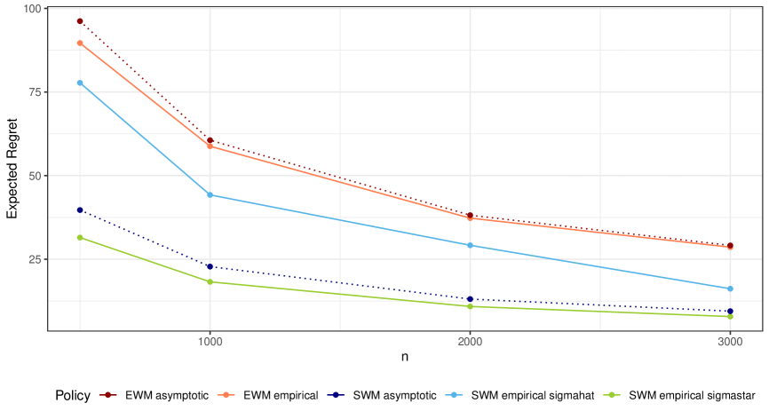
Figure 1: The figure illustrates asymptotic and finite sample expected regrets for the EWM and SWM policies in Model 1, corresponding to the values reported in Table 2.

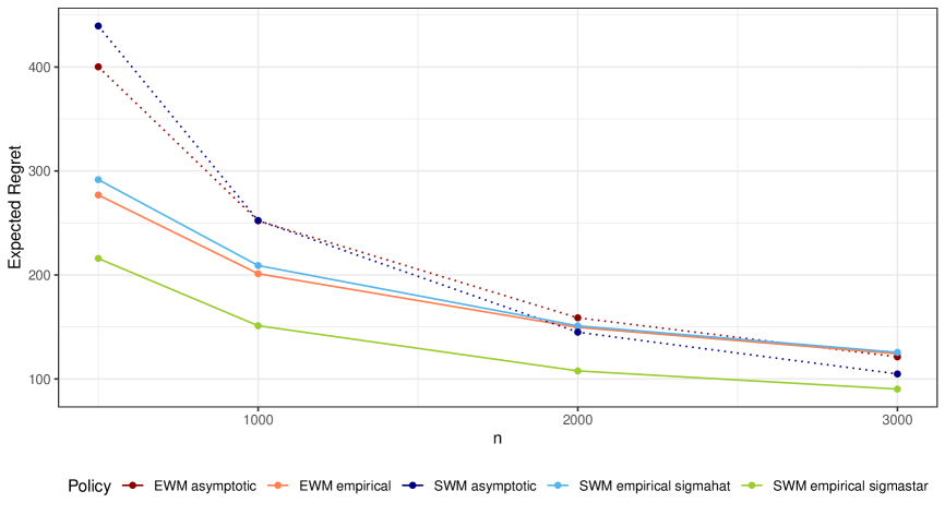
Figure 2: The figure illustrates asymptotic and finite sample expected regrets for the EWM and SWM policies in Model 2, corresponding to the values reported in Table 2.

Simulations enable comparison between finite sample regrets and their asymptotic counterparts. Across all models and sample sizes, the asymptotic approximation for the feasible SWM policy (with the estimated bandwidth $\hat{\sigma}_{n}^{*}$) is relatively less accurate. Simulations suggest that this is partly attributable to the need for estimating an additional tuning parameter, the bandwidth $\sigma_{n}$. When the SWM policy is estimated using the infeasible optimal bandwidth $\sigma^{*}_{n}$, in fact, the asymptotic approximation is more accurate and the regret is smaller.

In Model 1, as illustrated in Figure 1, both the finite sample and the asymptotic expected regrets are lower for the SWM policy. Conversely, in Model 2 (illustrated in Figure 2), the finite sample expected regret is lower with the EWM policy. This confirms the impossibility of ranking the policies in a pointwise sense: different distributions $P$ result in different rankings for the finite sample expected regrets.

It is important to note that the ranking of the EWM and the SWM policies indicated by the asymptotic results may differ from the actual finite sample comparison. Consider, for example, Model 2 with $n=2,000$: despite the asymptotic analysis suggesting a smaller expected regret with the SWM policy, the EWM actually guarantees a smaller regret. In this scenario, even if $P$ were known in advance, choosing according to the asymptotic approximation would not have been optimal. As $n$ increases, the approximation improves, and the rankings based on asymptotic analysis and finite sample comparisons coincide.

Monte Carlo simulations have confirmed that the asymptotic results can approximate some finite sample behavior of the regrets, highlighting some caveats to consider when applying conclusions from asymptotic analysis to finite sample regrets with the EWM and SWM policies. However, they have not yet provided insight into the practical significance of the differences between the two policies, whether these differences are relevant or negligible in real-world scenarios. An empirical illustration is useful to answer these questions, illustrating the different implications that the policies may have.

5 Empirical Illustration

I consider the same empirical setting as kitagawa2018should: experimental data from the National Job Training Partnership Act (JTPA) Study. bloom1997benefits describes the experiment in detail. The study randomized whether applicants would be eligible to receive a mix of training, job-search assistance, and other services provided by the JTPA for a period of 18 months. Background information on the applicants was collected before treatment assignment, alongside administrative and survey data on the applicants’ earnings over the subsequent 30 months.

I consider the same sample of 9,223 observations as in kitagawa2018should. The outcome variable $Y$ represents the total individual earnings during the 30 months following program assignment, and the treatment variable $D$ is a binary indicator denoting whether the individual was assigned to the program (intention-to-treat). The threshold policy is implemented by considering the individual’s earnings in the year preceding the assignment as the index $X$. Treatment is exclusively assigned to workers with prior earnings below the threshold, based on the expectation that program services yield a more substantial positive effect for individuals who previously experienced lower earnings. Experimental data are employed to determine the threshold beyond which the treatment, on average, harms the recipients.

The bandwidth to estimate the SWM policy is chosen as in the Monte Carlo simulation, using the EWM policy $\hat{t}^{e}_{n}$ to compute $\hat{A}_{n}$, $\hat{K}_{n}$, the optimal $\hat{\lambda}_{n}^{*}$, and then the optimal bandwidth $\hat{\sigma}_{n}^{*}$. Table 3 reports the threshold estimates, including the confidence intervals constructed as discussed in Appendix A. The threshold with the SWM policy is 700 dollars lower than with the EWM (5,924 vs 6,614 dollars), a drop of $10.5\%$. The lower threshold implies that the treatment would target fewer workers: if the EWM policy were implemented, $82.9\%$ of the workers in the sample would receive the program services, compared to the $78.9\%$ with the SWM policy, resulting in a $4$ percentage point decrease.

Table 3: Summary of the Empirical Welfare Maximizer (EWM) and Smoothed Welfare Maximizer (SWM) policies.

	EWM	SWM
Optimal threshold	6614	5924
Confidence interval	(4880.6, 8347.4)	(5832.7, 6411.3)
Bootstrapped confidence interval	(4748.5, 8060)
Expected asymptotic $\mathcal{R}$	41.299	5.296
Median asymptotic $\mathcal{R}$	19.47	2.597
% of workers treated	82.912	78.911

Results in corollaries 2.1 and 4.1 allow to estimate the expected and the median regret with the two policies: the asymptotic approximation suggests that the average regret drops from $42$ to $5.5$ dollars per worker, when comparing the EWM and SWM. In this context, the SWM would guarantee an average gain of $37.6$ dollars per worker over the 30-month period under study, equating to $909$ dollars on average for the workers who would change their treatment assignment under the two policies.

The numbers in the table should be considered with care, and clearly, the intention of this empirical illustration was not to advocate for a specific new job-training policy. Rather, the application aimed to assess if the EWM and SWM policies may have implications with relevant economic differences. Results suggest this is the case: together with theoretical and simulation findings, this implies that the choice between the EWM and the SWM policy should be thoughtfully considered, as it may determine relevant improvement in population welfare.

6 Conclusion

In this paper, I addressed the problem of using experimental data to estimate optimal threshold policies when the policymaker seeks to minimize the regret associated with implementing the policy in the population. I first examined the Empirical Welfare Maximizer threshold policy, deriving its asymptotic distribution, and showing how it links to the asymptotic distribution of its regret. I then introduced the Smoothed Welfare Maximizer policy, replacing the indicator function in the EWM policy with a smooth kernel function. Under the assumptions commonly made in the policy learning literature, the convergence rate for the worst-case regret of the SWM is faster than with the EWM policy. A comparative analysis of the asymptotic distributions of the two policies was conducted, to investigate how differently their regrets depend on the data distribution $P$. Monte Carlo simulations corroborated the asymptotic finding that the SWM policy may perform better than the commonly studied EWM policy also in finite sample. An empirical illustration displayed that the implications of the two policies can remarkably differ in real-world application.

Three sets of problems remain open for future research, to extend the results of this paper in diverse directions. While this study compared the EWM policy with its smoothed counterpart SWM, the literature in statistical decision theory has also examined alternative policy functions. Consider, for example, the Augmented Inverse Propensity Weighted policy proposed by athey2021policy: what is the asymptotic distribution of the AIPW policy’s regret in the context of threshold policies? How differently does it depend on $P$? Is it possible, analogously to what I did in this paper for the EWM policy, to modify the AIPW policy by smoothing the indicator function in its definition?

Second, it would be interesting to extend the smoothing approach from the EWM policy to other policy classes. Threshold policies are convenient as they depend on only one parameter. Still, besides more convoluted derivations, the same intuition of smoothing the indicator function also seems valid for the linear index or the multiple indices policy. The questions to explore include adapting the theory developed in this paper to these policy classes and whether this approach could be generalized even to all cases where the EWM policy is applied.

Lastly, the framework developed in this paper for using experimental data to estimate optimal policies could inform experimental design. While the existing literature mainly focuses on optimal design for estimating the average treatment effect, it could be valuable to consider scenarios when estimating the threshold policy is the goal: how should the experimental design be adapted? How the allocation of units to treatment and control groups would change? The results presented in this paper, elucidating the connection between the distribution $P$ and the regret of the policy, provide a natural foundation for exploring experimental designs optimal for threshold policy estimation.

Appendix A Confidence Intervals for Threshold Policies

Results derived in Section 3 can be used to construct confidence intervals that asymptotically cover the optimal threshold policy with a given probability, and to conduct hypotheses tests. It is important to remark that, in a decision problem setting, hypotheses testing does not have a clearly motivated justification, and indeed, statistical decision theory is the alternative approach to deal with decisions under uncertainty, as pointed out in manski2021econometrics. Rather than advocating for confidence intervals and hypothesis tests for threshold policies, this appendix aims to provide a procedure agnostic on why one may be interested in it.

For the EWM policy, rai2018statistical proposes some confidence intervals uniformly valid for several policy classes. They rely on test inversion of a certain bootstrap procedure, which compares the welfare generated by all the policies in the class. My procedure is much simpler for the EWM threshold policies, and I directly construct confidence intervals from the asymptotic distributions derived in Theorem 2. An analogous approach, built over results in Theorem 4, is then used to construct confidence intervals for the SWM policy.

A.1 Empirical Welfare Maximizer Policy

Consider the asymptotic distribution for the EWM threshold policy derived in Theorem 2:

$$n^{1/3}\left(\hat{t}^{e}_{n}-t^{*}\right)\rightarrow^{d}(2\sqrt{K}/H)^{2/3}\mathop{\rm arg~{}max}\limits_{r}\left(B(r)-r^{2}\right).$$ (16)

If $H$ and $K$ were known, confidence intervals for the optimal policy $t^{*}$ with asymptotic coverage $1-\alpha$ could be constructed as $(\hat{t}^{e}_{n}-w^{e}_{n},\hat{t}^{e}_{n}+w^{e}_{n})$, where

$$w^{e}_{n}=n^{-1/3}(2\sqrt{K}/H)^{2/3}c_{\alpha/2}$$ (17)

and $c_{\alpha/2}$ is the critical value, the upper $\alpha/2$ quantile of the distribution of $\max_{r}B(r)-r^{2}$.

In practice, $H$ and $K$ are unknown and should be estimated. They are defined as:

$$K= f_{x}(t^{*})\left(\frac{1}{p(\textbf{X})}\mathbb{E}[Y_{1}^{2}|X=t^{*}]+\frac{1}{1-p(\textbf{X})}\mathbb{E}[Y_{0}^{2}|X=t^{*}]\right)$$

$$H= f_{x}(t^{*})\left(\frac{\partial\mathbb{E}\left[Y_{1}-Y_{0}|X=t^{*}\right]}{\partial X}\right).$$

and can be estimated by a plug-in method: consider kernel density estimator $\hat{f}_{x}(x)$ for $f_{x}(x)$, and local linear estimators $\hat{\kappa}_{j}(x)$ and $\hat{\nu}_{j}^{\prime}(x)$ for $\kappa_{j}(x)=\mathbb{E}\left[Y_{j}^{2}|X=x,D=j\right]$ and $\nu_{j}^{\prime}(x)=\frac{\partial\nu_{j}(x)}{\partial x}=\frac{\partial\mathbb{E}\left[Y_{j}|X=x,D=j\right]}{\partial x}$. Define estimators $\hat{K}_{n}$ and $\hat{H}_{n}$ by:

$$\hat{K}_{n}=\hat{f}_{x}(\hat{t}^{e}_{n})\left(\frac{1}{p(\textbf{X})}\hat{\kappa}_{1}(\hat{t}^{e}_{n})+\frac{1}{1-p(\textbf{X})}\hat{\kappa}_{0}(\hat{t}^{e}_{n})\right)$$ (18)

and

$$\hat{H}_{n}=\hat{f}_{x}(\hat{t}^{e}_{n})(\hat{\nu}_{1}^{\prime}(\hat{t}^{e}_{n})-\hat{\nu}_{0}^{\prime}(\hat{t}^{e}_{n})).$$ (19)

Under the additional assumption that the second derivatives of $f_{x}$, $\nu_{1}$ and $\nu_{0}$ are continuous and bounded in a neighborhood of $t^{*}$, and with the proper choice of bandwidth sequences, $\hat{K}_{n}$ and $\hat{H}_{n}$ are consistent estimators for $K$ and $H$.

Feasible confidence intervals with asymptotic coverage $1-\alpha$ can hence be constructed as $(\hat{t}^{e}_{n}-\hat{w}^{e}_{n},\hat{t}^{e}_{n}+\hat{w}^{e}_{n})$, where

$$\hat{w}^{e}_{n}=n^{-1/3}(2\sqrt{\hat{K}_{n}}/\hat{H}_{n})^{2/3}c_{\alpha/2}.$$ (20)

A.1.1 Bootstrap

To avoid relying on tabulated values for $c_{\alpha/2}$ and on estimation of $K$, an alternative approach to inference for the EWM policy is the bootstrap. Nonparametric bootstrap is not valid for $\hat{t}^{e}_{n}$ and, more generally, for “cube root asymptotics” estimators (abrevaya2005bootstrap; leger2006bootstrap). Nonetheless, cattaneo2020bootstrap provide a consistent bootstrap procedure for estimators of this type. Consistency is achieved by altering the shape of the criterion function defining the estimator whose distribution must be approximated. The standard nonparametric bootstrap is inconsistent for $Q_{0}(r)=-\frac{1}{2}Hr$ as defined in the proof of Theorem 2, and hence the procedure in cattaneo2020bootstrap directly estimates this non-random part.

Let $\{Z_{i}^{b}\}$ be a random sample from the empirical distribution $P_{n}$, and define the estimator $\hat{t}^{b}_{n}$ as:

$$\hat{t}^{b}_{n}=\mathop{\rm arg~{}max}\limits_{t}\frac{1}{n}\sum_{i=1}^{n}\left[\left(\frac{D_{i}^{b}Y_{i}^{b}}{p(\textbf{X}_{i}^{b})}-\frac{(1-D_{i}^{b})Y_{i}^{b}}{(1-p(\textbf{X}_{i}^{b}))}\right)\mathbf{1}\{X_{i}^{b}>t\}\right]-$$ (21)

$$\frac{1}{n}\sum_{i=1}^{n}\left[\left(\frac{D_{i}Y_{i}}{p(\textbf{X}_{i})}-\frac{(1-D_{i})Y_{i}}{(1-p(\textbf{X}_{i}))}\right)\mathbf{1}\{X_{i}>t\}\right]-\frac{1}{2}(t-\hat{t}_{n})^{2}\hat{H}_{n}.$$ (22)

The bootstrap procedure proposed by cattaneo2020bootstrap is the following:

1. Compute $\hat{t}^{e}_{n}$ as described in equation (9).

2. Using $\hat{t}^{e}_{n}$, compute $\hat{H}_{n}$ as described in equation (19).

3. Using $\hat{t}^{e}_{n}$, $\hat{H}_{n}$, and the bootstrap sample $\{Z_{i}^{b}\}$, compute $\hat{t}^{b}_{n}$ as described in equation (21).

4. Iterate step 3 to obtain the distribution of $n^{1/3}\left(\hat{t}^{b}_{n}-\hat{t}^{e}_{n}\right)$, and use it as an estimate for the distribution of $n^{1/3}\left(\hat{t}^{e}_{n}-t^{*}\right)$.

To be valid, the procedure needs an additional assumption.

Assumption 6.

(Bounded 4th moment) Potential outcomes distribution are such that $\frac{1}{n^{2/3}}\mathbb{E}[Y_{1}^{4}|X=t^{*}]=o(1)$ and $\frac{1}{n^{2/3}}\mathbb{E}[Y_{0}^{4}|X=t^{*}]=o(1)$.

Assumption 6 guarantees that the envelope $G_{R}$ is such that $PG_{R}^{4}=o(R^{-1})$. Theorem 5 proves that the distribution of $n^{1/3}\left(\hat{t}^{b}_{n}-\hat{t}^{e}_{n}\right)$ consistently estimates the distribution of $n^{1/3}\left(\hat{t}^{e}_{n}-t^{*}\right)$, and validate the bootstrap procedure.

Theorem 5.

Consider estimators $\hat{t}^{e}_{n}$ defined in equation (9) and $\hat{t}^{b}_{n}$ defined in equation (21) and the estimand $t^{*}$ defined in equation (4). Under Assumptions 1, 2 with $s=2$, 3, and 6, as $\hat{H}_{n}\rightarrow^{p}H$ and $n\rightarrow\infty$,

$$n^{1/3}\left(\hat{t}^{b}_{n}-\hat{t}_{n}\right)\rightarrow^{d}(2\sqrt{K}/H)^{2/3}\mathop{\rm arg~{}max}\limits_{r}\left(B(r)-r^{2}\right)$$ (23)

where the limiting distribution is the same as in Theorem 2.

Distribution of $n^{1/3}\left(\hat{t}^{b}_{n}-\hat{t}^{e}_{n}\right)$ can hence be used to construct asymptotic valid confidence intervals and run hypothesis tests for $\hat{t}^{e}_{n}$.

A.2 Smoothed Welfare Maximizer Policy

Consider the asymptotic distribution for the SWM threshold policy derived in Theorem 4, for $n\sigma_{n}^{2h+1}\rightarrow\lambda<\infty$:

$$(n\sigma_{n})^{1/2}(\hat{t}^{s}_{n}-t^{*})\rightarrow^{d}\mathcal{N}(\lambda^{1/2}H^{-1}A,H^{-2}\alpha_{2}K).$$ (24)

$\lambda$, $\sigma_{n}$, and $\alpha_{2}$ are known. If also $K$, $H$, and $A$ were known, confidence intervals for the optimal policy $t^{*}$ with asymptotic coverage $1-\alpha$ could be constructed as $(\hat{t}^{s}_{n}-b_{n}-w^{s}_{n},\hat{t}^{s}_{n}-b_{n}+w^{s}_{n})$, where

$$b_{n}=(n\sigma_{n})^{-1/2}\lambda^{1/2}\frac{A}{H}$$ (25)

$$w^{s}_{n}=(n\sigma_{n})^{-1/2}(\sqrt{\alpha_{2}K}/H)c_{\alpha/2}$$ (26)

and $c_{\alpha/2}$ the upper $\alpha/2$ quantile of the standard normal distribution.

In practice, $K$, $H$, and $A$ are unknown and should be estimated. As usual with inference involving bandwidths and kernels, two approaches are available: estimate and remove the asymptotic bias, or undersmooth.

For the first approach, consider estimators in equation (18) for $\hat{K}_{n}$ and in equation (19) for $\hat{H}_{n}$, substituting $\hat{t}^{e}_{n}$ with $\hat{t}^{s}_{n}$. For $A$, recall that

$$A= -\frac{1}{h!}\alpha_{1}\int_{y}\left(Y_{1}-Y_{0}\right)\varphi^{h}_{x}(y,t^{*})dy$$ (27)

$$= -\frac{1}{h!}\alpha_{1}\left[2f^{\prime}_{x}(t^{*})[\lambda^{\prime}_{1}(t^{*})-\lambda^{\prime}_{0}(t^{*})]+f_{x}(t^{*})[\lambda^{\prime\prime}_{1}(t^{*})-\lambda^{\prime\prime}_{0}(t^{*})]\right]$$ (28)

where $f_{x}(x)$ is the probability density function of $X$ and $\nu_{j}(x)=\mathbb{E}[Y_{j}|X=x,D=j]$. Consider kernel density estimator $\hat{f}_{x}(x)$ and $\hat{f}^{\prime}_{x}(x)$ for $f_{x}(x)$ and $f^{\prime}_{x}(x)$, and local linear estimators $\hat{\nu}_{j}^{\prime}(x)$ and $\hat{\nu}_{j}^{\prime\prime}(x)$ for $\nu_{j}^{\prime}(x)=\frac{\partial\nu_{j}(x)}{\partial x}$ and $\nu_{j}^{\prime\prime}(x)=\frac{\partial^{2}\nu_{j}(x)}{\partial^{2}x}$. Define estimator $\hat{A}_{n}$ by:

$$\hat{A}_{n}=-\frac{1}{h!}\alpha_{1}\left[2\hat{f}^{\prime}_{x}(\hat{t}^{s}_{n})[\hat{\lambda}^{\prime}_{1}(\hat{t}^{s}_{n})-\hat{\lambda}^{\prime}_{0}(\hat{t}^{s}_{n})]+\hat{f}_{x}(\hat{t}^{s}_{n})[\hat{\lambda}^{\prime\prime}_{1}(\hat{t}^{s}_{n})-\hat{\lambda}^{\prime\prime}_{0}(\hat{t}^{s}_{n})]\right]$$ (29)

which consistently estimate $A$ the additional assumption that the third derivatives of $f_{x}$, $\nu_{1}$ and $\nu_{0}$ are continuous and bounded in a neighborhood of $t^{*}$, and with the proper choice of bandwidth sequences.

Confidence intervals with asymptotic coverage $1-\alpha$ can hence be constructed as $(\hat{t}^{s}_{n}-\hat{b}_{n}-\hat{w}^{s}_{n},\hat{t}^{s}_{n}-\hat{b}_{n}+\hat{w}^{s}_{n})$, where

$$\hat{b}_{n}=(n\sigma_{n})^{-1/2}\lambda^{1/2}\frac{\hat{A}_{n}}{\hat{H}_{n}}$$ (30)

$$\hat{w}^{s}_{n}=(n\sigma_{n})^{-1/2}(\sqrt{\alpha_{2}\hat{K}_{n}}/\hat{H}_{n})c_{\alpha/2}$$ (31)

The second approach relies on undersmoothing, and chooses a suboptimally small $\sigma_{n}$ to eliminate the asymptotic bias, with no need to estimate $A$. Instead of a bandwidth sequence $\sigma_{n}=O_{p}(n^{-\frac{1}{2h+1}})$, it considers a sequence $\sigma_{n}=o_{p}(n^{-\frac{1}{2h+1}})$ such that $n\sigma_{n}^{2h+1}\rightarrow\lambda=0$, and ensures $b_{n}\to 0$. Confidence intervals with asymptotic coverage $1-\alpha$ can hence be constructed as $(\hat{t}^{s}_{n}-\hat{w}^{s}_{n},\hat{t}^{s}_{n}+\hat{w}^{s}_{n})$, with $\hat{w}^{s}_{n}$ defined as above.

Appendix B Local Asymptotics

The interplay between the population distribution $P$ and the sample size can be studied considering a local asymptotic framework, considering a sequence of population distributions $\{P_{n}\}$ that varies with $n$. I focus on the following two sequences.

Definition 1.

(Sequence $\{P^{1}_{n}\}$) The sequence of distributions $\{P^{1}_{n}\}$ is such that $\frac{\sqrt{K_{n}}}{H_{n}}=n^{\gamma}$, with $\gamma\in[0,\frac{h}{2h+1})$, and $\frac{A_{n}}{H_{n}}=1$.

Definition 2.

(Sequence $\{P^{2}_{n}\}$) The sequence of distributions $\{P^{2}_{n}\}$ is such that $\frac{\sqrt{K_{n}}}{H_{n}}=1$, and $\frac{A_{n}}{H_{n}}=n^{\gamma}$, with $\gamma\in[0,\frac{h}{2h+1})$.

Sequence $\{P^{1}_{n}\}$ mimics a scenario where $\sqrt{K}$ is large compared to $H$. This occurs when the variance of the conditional treatment effect, $\operatorname{\mathrm{Var}}(Y_{1}-Y_{0}|X=t^{*})$, is large compared to the derivative of the conditional ATE, $\frac{\partial\mathbb{E}_{P}\left[Y_{1}-Y_{0}|X=t^{*}\right]}{\partial X}$, or compared to the density of the index, $f_{x}(t^{*})$. In these situations, the population welfare remains relatively stable for thresholds in the neighborhood of the optimal one. The limit case with $\gamma=\frac{1}{2}$ coincides with the local asymptotic framework proposed by hirano2009asymptotics and studied by athey2021policy.

Sequence $\{P^{2}_{n}\}$, instead, mimics a situation where $A$ is large compared to $H$. When $h=2$, this happens when the second derivative of the conditional ATE, $\frac{\partial^{2}\mathbb{E}_{P}\left[Y_{1}-Y_{0}|X=t^{*}\right]}{\partial^{2}X}$, is large compared to the first derivative, $\frac{\partial\mathbb{E}_{P}\left[Y_{1}-Y_{0}|X=t^{*}\right]}{\partial X}$. Since the asymptotic bias of $\hat{t}^{s}_{n}$ is $\lambda\frac{A_{n}}{H_{n}}$, sequence $\{P^{2}_{n}\}$ represents situation where this bias is large relatively to the sample size.

Let $r_{n}^{e}$ and $r_{n}^{s}$ denote the rates of convergence of $\mathcal{R}(\hat{t}^{e}_{n})$ and $\mathcal{R}(\hat{t}^{s}_{n})$, i.e. let $r_{n}^{e}$ and $r_{n}^{s}$ be sequences such that $\mathcal{R}(\hat{t}^{e}_{n})=O_{p}(r_{n}^{e})$ and $\mathcal{R}(\hat{t}^{s}_{n})=O_{p}(r_{n}^{s})$. The following theorem establishes a relationship between $r_{n}^{e}$ and $r_{n}^{s}$ under $\{P^{1}_{n}\}$ and $\{P^{2}_{n}\}$.

Theorem 6.

Let Assumptions 1, 2 with $s=h+1$ for some $h\geq 2$, 3, and 5 hold. Consider sequences $\{P^{1}_{n}\}$ and $\{P^{2}_{n}\}$ of data generating processes. The limit of the ratio $\frac{r_{n}^{e}}{r_{n}^{s}}$ depends on $\gamma$ as follows:

• $\frac{r_{n}^{e}}{r_{n}^{s}}\to\infty$ if $\gamma\in(\bar{\gamma},\frac{h}{2h+1})$

• $\frac{r_{n}^{e}}{r_{n}^{s}}=O_{p}(1)$ if $\gamma=\bar{\gamma}$

• $\frac{r_{n}^{e}}{r_{n}^{s}}\to 0$ if $\gamma\in[0,\bar{\gamma})$.

where $\bar{\gamma}=\frac{h-1}{2h+1}$ under $\{P^{1}_{n}\}$, and $\bar{\gamma}=\frac{1}{3}\frac{h-1}{2h+1}$ under $\{P^{2}_{n}\}$.

Theorem 6 shows how, under sequences $\{P^{1}_{n}\}$ and $\{P^{2}_{n}\}$, the EWM policy guarantees a regret convergence rate faster than the SWM policy whenever the parameter $\gamma$ exceeds a certain value $\bar{\gamma}$. For sequence $\{P^{1}_{n}\}$, the result depends on the fact that the term $\frac{\sqrt{K_{n}}}{H_{n}}$ enters the asymptotic distributions of $\hat{t}^{e}_{n}$ and $\hat{t}^{s}_{n}$ with different powers ($\frac{2}{3}$ and 1, respectively): if $\frac{\sqrt{K_{n}}}{H_{n}}$ is large enough relatively to the sample size, the exponent lower than one makes $r^{e}_{n}$ faster (and hence in the limit $\hat{t}^{e}_{n}$ preferable). For sequence $\{P^{2}_{n}\}$, the result is due to the asymptotic bias of the SWM policy, proportional to $\frac{A_{n}}{H_{n}}$. Since the asymptotic distribution of the regret of the EWM policy remains constant in $\{P^{2}_{n}\}$, when the bias of $\hat{t}^{s}_{n}$ is large enough compared to sample size, $\hat{t}^{e}_{n}$ becomes preferable. The value of $\bar{\gamma}$ is increasing in $h$, the order of the kernel $k$: a smoother objective function $\mathbb{E}[(Y_{1}-Y_{0})\mathbf{1}\{X>t\}]$ amplifies the benefit of using the SWM policy, expanding the region of values of $\gamma$ where the SWM policy has a faster rate compared to the EWM.

Considering the sequence $\{P^{1}_{n}\}$ with $\gamma=\frac{1}{2}$, athey2021policy show that their AIPW policy achieves the uniform fastest asymptotic convergence rate. Results in Theorem 6 are different: without focusing on a single specific sequence, their goal is to shed light on how the asymptotic behavior of the EWM and the SWM policies depends on $P$ and sample size.

Appendix C Monte Carlo Simulation

I report the analogous of Table 2 and Figures 1 and 2 for the median regret. Comments made for the mean also extend to the median regret.

Table 4: Finite sample and asymptotic median regret with the EWM and SWM policies across different models. Finite sample (empirical) values are computed through 5,000 Monte Carlo simulations. The last column reports the ratio between finite sample median regrets with the EWM and SWM policies.

Model	n	EWM		SWM			Ratio
		empirical	asymptotic	empirical $\sigma_{n}^{*}$	empirical $\hat{\sigma}_{n}^{*}$	asymptotic
1	$500$	$39.809$	$45.347$	$15.113$	$24.169$	$18.459$	$1.647$
	$1,000$	$27.547$	$28.567$	$8.692$	$14.145$	$10.602$	$1.948$
	$2,000$	$18.816$	$17.996$	$5.073$	$8.507$	$6.089$	$2.212$
	$3,000$	$14.043$	$13.733$	$3.471$	$5.491$	$4.402$	$2.558$
2	$500$	$147.029$	$188.651$	$116.784$	$159.876$	$204.255$	$0.920$
	$1,000$	$110.372$	$118.843$	$82.473$	$118.695$	$117.314$	$0.930$
	$2,000$	$87.325$	$74.866$	$55.731$	$79.436$	$67.379$	$1.099$
	$3,000$	$72.122$	$57.134$	$46.007$	$68.656$	$48.714$	$1.050$

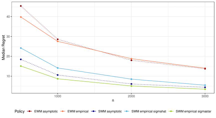
Figure 3: Figure reports asymptotic and finite sample median regrets for the EWM and SWM policies, illustrating the values reported in Table 4.

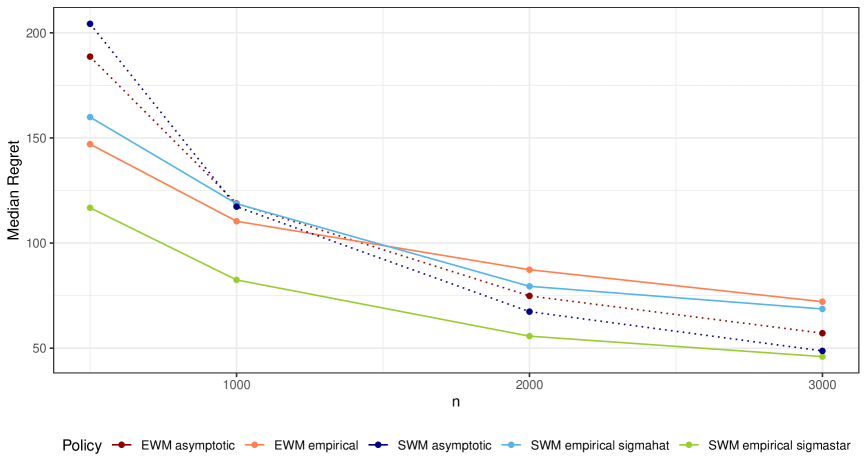
Figure 4: Figure reports asymptotic and finite sample median regrets for the EWM and SWM policies, illustrating the values reported in Table 4.

Appendix D Proofs

Theorem 1

Theorem 1.

Consider the EWM policy $\hat{t}^{e}_{n}$ defined in equation (9) and the optimal policy $t^{*}$ defined in equation (4). Under Assumptions 1 and 2 with $s=0$,

$$\hat{t}^{e}_{n}\rightarrow^{a.s.}t^{*}$$

i.e. $\hat{t}^{e}_{n}$ is a consistent estimator for $t^{*}$.

Proof.

Estimator $\hat{t}^{e}_{n}$ in (9) can be written as

$$\hat{t}^{e}_{n}= \mathop{\rm arg~{}max}\limits_{t}\frac{1}{n}\sum_{i=1}^{n}\left[\left(\frac{D_{i}Y_{i}}{p(\textbf{X}_{i})}-\frac{(1-D_{i})Y_{i}}{(1-p(\textbf{X}_{i}))}\right)(\mathbf{1}\{X_{i}>t\}-\mathbf{1}\{X_{i}>t^{*}\})\right]$$ (32)

$$= \mathop{\rm arg~{}max}\limits_{t}\frac{1}{n}\sum_{i=1}^{n}m\left(Z_{i},t\right)$$ (33)

where

$$m\left(Z,t\right)=\left(\frac{DY}{p(\textbf{X})}-\frac{(1-D)Y}{(1-p(\textbf{X}))}\right)\left(\mathbf{1}\{X>t\}-\mathbf{1}\{X>t^{*}\}\right)$$ (34)

and $\{Z_{i}\}$ is a sample of $n$ observation from distribution $P$.

Define $P_{n}m\left(\cdot,t\right)=\sum_{i=1}^{n}m\left(Z_{i},t\right)$ and $Pm\left(Z,t\right)=\mathbb{E}_{P}[m\left(Z,t\right)]$. With this notation, equation (4) and (9) can be written as

$$t^{*}=\mathop{\rm arg~{}max}\limits_{t}Pm\left(Z,t\right)$$ (35)

$$\hat{t}^{e}_{n}=\mathop{\rm arg~{}max}\limits_{t}P_{n}m\left(\cdot,t\right).$$ (36)

Threshold policies I am considering can be seen as a tree partition of depth 1. Tree partitions of finite depth are a VC class (leboeuf2020decision), and hence $m\left(\cdot,t\right)$ is a manageable class of functions. Consider the envelope function $F=2\left|\frac{DY}{p(\textbf{X})}-\frac{(1-D)Y}{(1-p(\textbf{X}))}\right|$. Note that $\mathbb{E}\left[\left|\frac{DY}{p(\textbf{X})}-\frac{(1-D)Y}{(1-p(\textbf{X}))}\right|^{2}\right]=\frac{1}{p(\textbf{X})}\mathbb{E}[Y_{1}^{2}]+\frac{1}{1-p(\textbf{X})}\mathbb{E}[Y_{0}^{2}]$: Assumption 2.2 guarantees the existence of $\mathbb{E}\left[\left|\frac{DY}{p(\textbf{X})}-\frac{(1-D)Y}{(1-p(\textbf{X}))}\right|^{2}\right]$.

It follows from corollary 3.2 in kim1990cube that

$$\sup_{t}\left|P_{n}m(\cdot,t)-Pm(Z,t)\right|\rightarrow^{a.s.}0.$$ (37)

Under Assumptions 2.1 and 2.3, $Pm(Z,t)$ is continuous in $t$, and $t^{*}$ is the unique maximizer. Hence,

$$\sup_{t}\left|P_{n}m(\cdot,t)-Pm(Z,t)\right|+Pm(Z,t^{*})\geq$$ (38)

$$\left|P_{n}m(\cdot,\hat{t}^{e}_{n})-Pm(Z,\hat{t}^{e}_{n})\right|+Pm(Z,t^{*})\geq$$ (39)

$$\left|P_{n}m(\cdot,\hat{t}^{e}_{n})-Pm(Z,\hat{t}^{e}_{n})\right|+Pm(Z,\hat{t}^{e}_{n})\geq$$ (40)

$$P_{n}m(\cdot,\hat{t}^{e}_{n})\geq P_{n}m(\cdot,t^{*})\rightarrow Pm(Z,t^{*})$$ (41)

where the second inequality is due to the fact that $t^{*}$ is the maximizer of $Pm(Z,t)$, the third comes from the triangular inequality, the fourth from $\hat{t}^{e}_{n}$ being the maximizer of $P_{n}m(\cdot,t)$, and the last limit comes from LLN. This prove that $P_{n}m(\cdot,\hat{t}^{e}_{n})\rightarrow^{a.s.}Pm(Z,t^{*})$, and hence $Pm(Z,\hat{t}^{e}_{n})\rightarrow^{a.s.}Pm(Z,t^{*})$. Since $t^{*}$ is the unique maximizer of $Pm(Z,t)$ and $Pm(Z,t)$ is continuous, $\hat{t}^{e}_{n}\rightarrow^{a.s.}t^{*}$. It means that $\hat{t}^{e}_{n}$ is a consistent estimator for $t^{*}$. ∎

Theorem 2

Theorem 2.

Consider the EWM policy $\hat{t}^{e}_{n}$ defined in equation (9) and the optimal policy $t^{*}$ defined in equation (4). Under Assumptions 1, 2 with $s=2$ and 3, as $n\rightarrow\infty$,

$$n^{1/3}\left(\hat{t}^{e}_{n}-t^{*}\right)\rightarrow^{d}(2\sqrt{K}/H)^{2/3}\mathop{\rm arg~{}max}\limits_{r}\left(B(r)-r^{2}\right)$$ (42)

where $B(r)$ is the two-sided Brownian motion process, and $K$ and $H$ are

$$K= f_{x}(t^{*})\left(\frac{1}{p(\textbf{X})}\mathbb{E}[Y_{1}^{2}|X=t^{*}]+\frac{1}{1-p(\textbf{X})}\mathbb{E}[Y_{0}^{2}|X=t^{*}]\right)$$

$$H= f_{x}(t^{*})\left(\frac{\partial\mathbb{E}_{P}\left[Y_{1}-Y_{0}|X=t^{*}\right]}{\partial X}\right).$$

Proof.

The proof shows that conditions for the main theorem in kim1990cube hold; hence, their result is valid for $\hat{t}^{e}_{n}$. For completeness, I report the theorem.

Theorem Kim and Pollard.

Consider estimators defined by maximization of processes

$$P_{n}g(\cdot,\theta)=\frac{1}{n}\sum_{i=1}^{n}g\left(\xi_{i},\theta\right)$$ (43)

where $\left\{\xi_{i}\right\}_{i}$ is a sequence of i.i.d. observations from a distribution $P$ and $\{g(\cdot,\theta):\theta\in\Theta\}$ is a class of functions indexed by a subset $\Theta$ in $\mathbb{R}^{k}$. The envelope $G_{R}(\cdot)$ is defined as the supremum of $g(\cdot,\theta)$ over the class

$$\mathcal{G}_{R}=\left\{|g(\cdot,\theta)|:\left|\theta-\theta_{0}\right|\leq R\right\},\quad R>0.$$ (44)

Let $\left\{\theta_{n}\right\}$ be a sequence of estimators for which

1. $P_{n}g\left(\cdot,\theta_{n}\right)\geq\sup_{\theta\in\Theta}P_{n}g(\cdot,\theta)-o_{P}\left(n^{-2/3}\right)$.

2. $\theta_{n}$ converges in probability to the unique $\theta_{0}$ that maximizes $Pg(\cdot,\theta)$.

3. $\theta_{0}$ is an interior point of $\Theta$.

Let the functions be standardized so that $g\left(\cdot,\theta_{0}\right)\equiv 0$. If the classes $\mathcal{G}_{R}$ for $R$ near 0 are uniformly manageable for the envelopes $G_{R}$ and satisfy:

1. $Pg(\cdot,\theta)$ is twice differentiable with second derivative matrix $-H$ at $\theta_{0}$.

2. $K(s,r)=\lim_{\alpha\rightarrow\infty}\alpha Pg\left(\cdot,\theta_{0}+r/\alpha\right)g\left(\cdot,\theta_{0}+s/\alpha\right)$ exists for each $s,r$ in $\mathbb{R}^{k}$ and $\lim_{\alpha\rightarrow\infty}\alpha Pg\left(\cdot,\theta_{0}+r/\alpha\right)^{2}\left\{\left|g\left(\cdot,\theta_{0}+r/\alpha\right)\right|>\varepsilon\alpha\right\}=0$ for each $\varepsilon>0$ and $r$ in $\mathbb{R}^{k}$.

3. $PG_{R}^{2}=O(R)$ as $R\rightarrow 0$ and for each $\varepsilon>0$ there is a constant C such that $PG_{R}^{2}\mathbf{1}\{G_{R}>C\}\leq\varepsilon R$ for $R$ near 0.

4. $P\left|g\left(\cdot,\theta_{1}\right)-g\left(\cdot,\theta_{2}\right)\right|=O\left(\left|\theta_{1}-\theta_{2}\right|\right)$ near $\theta_{0}$.

Then, the process $n^{2/3}P_{n}g\left(\cdot,\theta_{0}+rn^{-1/3}\right)$ converges in distribution to a Gaussian process $Q(r)$ with continuous sample paths, expected value $-\frac{1}{2}r^{\prime}Hr$ and covariance kernel $K$. If $H$ is positive definite and if $Q$ has nondegenerate increments, then $n^{1/3}\left(\theta_{n}-\theta_{0}\right)$ converges in distribution to the (almost surely unique) random vector that maximizes $Q$.

I apply Theorem Theorem Kim and Pollard by taking $\xi_{i}=Z_{i},\theta=t,\theta_{n}=\hat{t}^{e}_{n},\theta_{0}=t^{*}$, $g(\cdot,\theta)=m(\cdot,t)$, where $m(\cdot,t)$ is standardized:

$$m\left(Z_{i},t\right)=\left(\frac{D_{i}Y_{i}}{p(\textbf{X}_{i})}-\frac{(1-D_{i})Y_{i}}{(1-p(\textbf{X}_{i}))}\right)\left(\mathbf{1}\{X_{i}>t\}-\mathbf{1}\{X_{i}>t^{*}\}\right).$$ (45)

First, I will verify that conditions 1-7 apply to my setting:

1. $P_{n}m(\cdot,t)$ takes only finite ($n+1$) values; hence, condition 1 is satisfied with the equality.

2. In Theorem 1, I proved that $\hat{t}^{e}_{n}$ is a consistent estimator for $t^{*}$.

3. $t^{*}$ is an interior point of $\mathcal{T}$ by Assumption 2.1.

I need to prove that the classes $\mathcal{G}_{R}$ for $R$ near 0 are uniformly manageable for the envelopes $G_{R}$. The envelope function $G_{R}(\cdot)$ is defined as

$$G_{R}(z) =\sup\left\{m(z,t):\left|t-t^{*}\right|\leq R\right\}$$ (46)

$$=\sup_{\left|t-t^{*}\right|\leq R}\left[\left(\frac{dy}{p(\textbf{x})}-\frac{(1-d)y}{(1-p(\textbf{x}))}\right)\left(\mathbf{1}\{x>t\}-\mathbf{1}\{x>t^{*}\}\right)\right]$$ (47)

$$=\left|\frac{dy}{p(\textbf{x})}-\frac{(1-d)y}{(1-p(\textbf{x}))}\right|\mathbf{1}\{\left|x-t^{*}\right|<R\}$$ (48)

and I have:

$$PG_{R}^{2} =\mathbb{E}\left[\left(\frac{DY}{p(\textbf{X})}-\frac{(1-D)Y}{(1-p(\textbf{X}))}\right)^{2}\mathbf{1}\{\left|X-t^{*}\right|<R\}\right]$$ (49)

$$=\mathbb{E}\left[\left(\frac{DY}{p(\textbf{X})}-\frac{(1-D)Y}{(1-p(\textbf{X}))}\right)^{2}\Bigg{|}X\in(t^{*}-R,t^{*}+R)\right]$$ (50)

$$=2R\mathbb{E}\left[\left(\frac{DY}{p(\textbf{X})}-\frac{(1-D)Y}{(1-p(\textbf{X}))}\right)^{2}\Bigg{|}X=t^{*}\right]+o(1)=O(R)$$ (51)

where the second to last equality comes from Assumption 2.2. The envelope function is uniformly square-integrable for $R$ near 0, and therefore, the classes $\mathcal{G}_{R}$ are uniformly manageable.

1. Define $h(t)=Pm(Z,t)$ and consider derivatives:

   $$h(t)= \mathbb{E}_{P}\left[\left(\frac{DY}{p(\textbf{X})}-\frac{(1-D)Y}{(1-p(\textbf{X}))}\right)(\mathbf{1}\{X>t\}-\mathbf{1}\{X>t^{*}\})\right]=$$ (52)

   $$\mathbb{E}_{P}\left[\left(Y_{1}-Y_{0}\right)(\mathbf{1}\{X>t\}-\mathbf{1}\{X>t^{*}\})\right]$$ (53)

   $$h^{\prime}(t)= -f_{x}(t)\mathbb{E}_{P}\left[Y_{1}-Y_{0}\Big{|}X=t\right]$$ (54)

   $$h^{\prime\prime}(t)= -f^{\prime}_{x}(t)\mathbb{E}_{P}\left[Y_{1}-Y_{0}\Big{|}X=t\right]-f_{x}(t)\left(\frac{\partial\mathbb{E}_{P}\left[Y_{1}-Y_{0}|X=t\right]}{\partial X}\right).$$ (55)

   Assumption 2.3 with $s=2$ guarantees the existence of $h^{\prime}$ and $h^{\prime\prime}$. Since $\mathbb{E}_{P}\left[Y_{1}-Y_{0}\Big{|}X=t^{*}\right]=0$, $H$ is given by

   $$H=-h^{\prime\prime}(t^{*})=f_{x}(t^{*})\left(\frac{\partial\mathbb{E}_{P}\left[Y_{1}-Y_{0}|X=t^{*}\right]}{\partial X}\right).$$ (56)

2. This condition is divided into two parts. First, I prove the existence of $K(s,r)=\lim_{\alpha\rightarrow\infty}\alpha Pm\left(\cdot,t^{*}+r/\alpha\right)m\left(\cdot,t^{*}+s/\alpha\right)$ for each $s,r$ in $\mathbb{R}$. Covariance $K$ is:

   $$Pm \left(\cdot,t^{*}+r/\alpha\right)m\left(\cdot,t^{*}+s/\alpha\right)=\mathbb{E}\left[\left(\frac{DY}{p(\textbf{X})}-\frac{(1-D)Y}{(1-p(\textbf{X}))}\right)^{2}\right.$$ (57)

   $$(\mathbf{1}\{X>t^{*}+r/\alpha\}-\mathbf{1}\{X>t^{*}\})(\mathbf{1}\{X>t^{*}+s/\alpha\}-\mathbf{1}\{X>t^{*}\})\Big{]}.$$ (58)

   If $rs<0$, covariance and $K(s,r)$ are 0. If $rs>0$, and suppose $r>0$:

   $$Pm\left(\cdot,t^{*}+r/\alpha\right)m\left(\cdot,t^{*}+s/\alpha\right)=$$ (59)

   $$\mathbb{E}\left[\left(\frac{DY}{p(\textbf{X})}-\frac{(1-D)Y}{(1-p(\textbf{X}))}\right)^{2}\Big{|}X\in(t^{*},t^{*}+\min\{r,s\}/\alpha)\right]$$ (60)

   and hence

   $$K(s,r) =\lim_{\alpha\rightarrow\infty}\alpha\mathbb{E}\left[\left(\frac{DY}{p(\textbf{X})}-\frac{(1-D)Y}{(1-p(\textbf{X}))}\right)^{2}\Big{|}X\in(t^{*},t^{*}+\min\{r,s\}/\alpha)\right]$$ (61)

   $$=\min\{r,s\}f_{x}(t^{*})\mathbb{E}\left[\left(\frac{DY}{p(\textbf{X})}-\frac{(1-D)Y}{(1-p(\textbf{X}))}\right)^{2}\Big{|}X=t^{*}\right].$$ (62)

   where the equality is due to continuity of $f_{x}$ (Assumption 2.3 with $s=2$). Boundedness of the quantity follows from Assumptions 2.2 and 2.3.

   Now, I will prove that $\lim_{\alpha\rightarrow\infty}\alpha Pm\left(\cdot,t^{*}+r/\alpha\right)^{2}\mathbf{1}\left\{\left|m\left(\cdot,t^{*}+r/\alpha\right)\right|>\varepsilon\alpha\right\}=0$ for each $\varepsilon>0$ and $r$ in $\mathbb{R}$. I have:

   $$\alpha Pm\left(\cdot,t^{*}+r/\alpha\right)^{2}\mathbf{1}\left\{\left|m\left(\cdot,t^{*}+r/\alpha\right)\right|>\varepsilon\alpha\right\}=$$ (63)

   $$\alpha\mathbb{E}\left[\left(\frac{DY}{p(\textbf{X})}-\frac{(1-D)Y}{(1-p(\textbf{X}))}\right)^{2}\right.$$ (64)

   $$(\mathbf{1}\{X>t^{*}+r/\alpha\}-\mathbf{1}\{X>t^{*}\})^{2}\mathbf{1}\left\{\left|m\left(\cdot,t^{*}+r/\alpha\right)\right|>\varepsilon\alpha\right\}\Big{]}=$$ (65)

   $$\alpha\mathbb{E}\left[\left(\frac{DY}{p(\textbf{X})}-\frac{(1-D)Y}{(1-p(\textbf{X}))}\right)^{2}\right.$$ (66)

   $$(\mathbf{1}\{X>t^{*}+r/\alpha\}-\mathbf{1}\{X>t^{*}\})^{2}\mathbf{1}\left\{\left|\frac{DY}{p(\textbf{X})}-\frac{(1-D)Y}{(1-p(\textbf{X}))}\right|>\varepsilon\alpha\right\}\Big{]}\leq$$ (67)

   $$\alpha\mathbb{E}\left[\left(\frac{DY}{p(\textbf{X})}-\frac{(1-D)Y}{(1-p(\textbf{X}))}\right)^{2}\mathbf{1}\left\{\left|\frac{DY}{p(\textbf{X})}-\frac{(1-D)Y}{(1-p(\textbf{X}))}\right|>\varepsilon\alpha\right\}\right].$$ (68)

   Some algebra gives

   $$\mathbb{E}\left[\left(\frac{DY}{p(\textbf{X})}-\frac{(1-D)Y}{(1-p(\textbf{X}))}\right)^{2}\mathbf{1}\left\{\left|\frac{DY}{p(\textbf{X})}-\frac{(1-D)Y}{(1-p(\textbf{X}))}\right|>\epsilon\right\}\right]=$$ (69)

   $$\mathbb{E}\left[\left(\frac{DY_{1}^{2}}{p(\textbf{X})^{2}}+\frac{(1-D)Y_{0}^{2}}{(1-p(\textbf{X}))^{2}}\right)\mathbf{1}\left\{\left|\frac{DY}{p(\textbf{X})}-\frac{(1-D)Y}{(1-p(\textbf{X}))}\right|>\epsilon\right\}\right]=$$ (70)

   $$\mathbb{E}\left[\frac{Y_{1}^{2}}{p(\textbf{X})}\mathbf{1}\left\{\left|\frac{Y_{1}}{p(\textbf{X})}\right|>\epsilon\right\}\right]+\mathbb{E}\left[\frac{Y_{0}^{2}}{(1-p(\textbf{X}))}\mathbf{1}\left\{\left|\frac{Y_{0}}{(1-p(\textbf{X}))}\right|>\epsilon\right\}\right]=$$ (71)

   $$\frac{1}{p(\textbf{X})}\mathbb{E}\left[Y_{1}^{2}\mathbf{1}\left\{\left|Y_{1}\right|>\epsilon_{1}\right\}\right]+\frac{1}{(1-p(\textbf{X}))}\mathbb{E}\left[Y_{0}^{2}\mathbf{1}\left\{\left|Y_{0}\right|>\epsilon_{0}\right\}\right]$$ (72)

   and hence the condition is satisfied if

   $$\lim_{\alpha\rightarrow\infty}\alpha\mathbb{E}\left[Y_{1}^{2}\mathbf{1}\left\{\left|Y_{1}\right|>\epsilon\alpha\right\}\right]=0$$ (73)

   $$\lim_{\alpha\rightarrow\infty}\alpha\mathbb{E}\left[Y_{0}^{2}\mathbf{1}\left\{\left|Y_{0}\right|>\epsilon\alpha\right\}\right]=0.$$ (74)

   Consider the limit for $Y_{1}$:

   $$\lim_{\alpha\rightarrow\infty}\alpha\mathbb{E}\left[Y_{1}^{2}\mathbf{1}\left\{\left|Y_{1}\right|>\epsilon\alpha\right\}\right]=\lim_{\alpha\rightarrow\infty}\frac{\int_{\epsilon\alpha}Y_{1}^{2}\varphi_{1}(y_{1})dy_{1}}{\alpha^{-1}}=\lim_{\alpha\rightarrow\infty}\frac{\epsilon^{3}\alpha^{2}\varphi_{1}(\epsilon\alpha)}{\alpha^{-2}}=$$ (75)

   $$\lim_{\alpha\rightarrow\infty}\epsilon^{3}\alpha^{4}\varphi_{1}(\epsilon\alpha)=\lim_{\alpha\rightarrow\infty}\epsilon^{3}\alpha^{4}|\epsilon\alpha|^{-(4+\delta)}o(1)=0$$ (76)

   where the second to last equality follows from Assumption 3.

3. I showed that $PG_{R}^{2}=O(R)$ as $R\rightarrow 0$ in equation (49). I need to prove that for each $\varepsilon>0$ there is a constant C such that $PG_{R}^{2}\mathbf{1}\{G_{R}>C\}\leq\varepsilon R$ for $R$ near 0. For any $\varepsilon>0$ and $C>0$:

   $$PG_{R}^{2} \mathbf{1}\{G_{R}>C\}=\mathbb{E}\left[\left(\frac{DY}{p(\textbf{X})}-\frac{(1-D)Y}{(1-p(\textbf{X}))}\right)^{2}\mathbf{1}\{\left|X-t^{*}\right|<R\}\mathbf{1}\{G_{R}>C\}\right]\leq$$ (77)

   $$\mathbb{E}\left[\left(\frac{DY}{p(\textbf{X})}-\frac{(1-D)Y}{(1-p(\textbf{X}))}\right)^{2}\mathbf{1}\{\left|X-t^{*}\right|<R\}\mathbf{1}\left\{\left|\frac{DY}{p(\textbf{X})}-\frac{(1-D)Y}{(1-p(\textbf{X}))}\right|>C\right\}\right]\leq$$ (78)

   $$\mathbb{E}\left[\left(\frac{DY}{p(\textbf{X})}-\frac{(1-D)Y}{(1-p(\textbf{X}))}\right)^{2}\mathbf{1}\left\{\left|\frac{DY}{p(\textbf{X})}-\frac{(1-D)Y}{(1-p(\textbf{X}))}\right|>C\right\}\right]\rightarrow 0$$ (79)

   where the last limit is taken for $C\rightarrow\infty$, and follows from Assumption 3.

4. I need to show that $P\left|m\left(\cdot,t_{1}\right)-m\left(\cdot,t_{2}\right)\right|=O\left(\left|t_{1}-t_{2}\right|\right)$ near $t^{*}$. Consider $t_{2}>t_{1}$:

   $$P\left|m\left(\cdot,t_{1}\right)-m\left(\cdot,t_{2}\right)\right|=\mathbb{E}\left[\left|\left(\frac{DY}{p(\textbf{X})}-\frac{(1-D)Y}{(1-p(\textbf{X}))}\right)(\mathbf{1}\{X>t_{1}\}-\mathbf{1}\{X>t_{2}\})\right|\right]\leq$$ (80)

   $$M_{x}\mathbb{E}\left[\left|\left(\frac{DY}{p(\textbf{X})}-\frac{(1-D)Y}{(1-p(\textbf{X}))}\right)\right|\Big{|}X\in(t_{1},t_{2})\right]\leq M_{x}M_{y}|t_{2}-t_{1}|$$ (81)

   where $M_{x}=\max_{x\in(t_{1},t_{2})}f_{x}(x)$ and $M_{y}=\max_{x\in(t_{1},t_{2})}\mathbb{E}\left[\left|\left(\frac{DY}{p(\textbf{X})}-\frac{(1-D)Y}{(1-p(\textbf{X}))}\right)\right|\Big{|}X\right]$. $M_{x}<\infty$ and $M_{y}<\infty$ because of Assumption 2.3.

Assumptions 1-7 of Theorem Theorem Kim and Pollard by kim1990cube are hence satisfied. It follows that, for $n\rightarrow\infty$,

$$n^{1/3}\left(\hat{t}^{e}_{n}-t^{*}\right)\rightarrow^{d}\mathop{\rm arg~{}max}\limits_{r}Q(r)$$ (82)

where $Q(r)=Q_{1}(r)+Q_{0}(r)$, and $Q_{1}$ is a non degenerate zero-mean Gaussian process with covariance $K$, while $Q_{0}(r)$ is non-random and $Q_{0}(r)=-\frac{1}{2}r^{2}H$.

Limiting distribution $\mathop{\rm arg~{}max}\limits_{r}Q(r)$ is of chernoff1964estimation type. It can be shown (banerjee2001likelihood) that

$$\mathop{\rm arg~{}max}\limits_{r}Q(r)=^{d}(2\sqrt{K}/H)^{2/3}\mathop{\rm arg~{}max}\limits_{r}B(r)-r^{2}$$ (83)

where $B(r)$ is the two-sided Brownian motion process, $K$ is:

$$K= f_{x}(t^{*})\mathbb{E}\left[\left(\frac{DY}{p(\textbf{X})}-\frac{(1-D)Y}{(1-p(\textbf{X}))}\right)^{2}\Big{|}X=t^{*}\right]$$ (84)

$$= f_{x}(t^{*})\left(\frac{1}{p(\textbf{X})}\mathbb{E}[Y_{1}^{2}|X=t^{*}]+\frac{1}{1-p(\textbf{X})}\mathbb{E}[Y_{0}^{2}|X=t^{*}]\right)$$ (85)

and $H$ is:

$$H=f_{x}(t^{*})\left(\frac{\partial\mathbb{E}_{P}\left[Y_{1}-Y_{0}|X=t^{*}\right]}{\partial X}\right).$$ (86)

This completes the proof of the theorem. ∎

Corollary 2.1

Corollary 2.1.

The asymptotic distribution of regret $\mathcal{R}(\hat{t}^{e}_{n})$ is:

$$n^{\frac{2}{3}}\mathcal{R}(\hat{t}^{e}_{n})\rightarrow^{d}\left(\frac{2K^{2}}{H}\right)^{\frac{1}{3}}\left(\mathop{\rm arg~{}max}\limits_{r}B(r)-r^{2}\right)^{2}.$$

The expected value of the asymptotic distribution is $K^{\frac{2}{3}}H^{-\frac{1}{3}}C^{e}$, where

$$C^{e}=\sqrt[3]{2}\mathbb{E}\left[\left(\mathop{\rm arg~{}max}\limits_{r}B(r)-r^{2}\right)^{2}\right]$$

is a constant not dependent on $P$.

Proof.

Result in equation (6) for $\hat{t}^{e}_{n}$ implies

$$n^{\frac{2}{3}}\mathcal{R}(\hat{t}^{e}_{n})=\frac{1}{2}W^{\prime\prime}(\tilde{t})\left(n^{\frac{1}{3}}\left(\hat{t}^{e}_{n}-t^{*}\right)\right)^{2},$$

where $|\tilde{t}-t^{*}|\leq|\hat{t}_{n}-t^{*}|$. By continuous mapping theorem

$$W^{\prime\prime}(\tilde{t})\rightarrow^{p}W^{\prime\prime}(t^{*})=H$$

and hence by Slutsky’s theorem

$$n^{\frac{2}{3}}\left(W(\hat{t}_{n})-W(t^{*})\right)\rightarrow^{d}\left(\frac{2K^{2}}{H}\right)^{\frac{1}{3}}\left(\mathop{\rm arg~{}max}\limits_{r}B(r)-r^{2}\right)^{2}.$$

∎

Theorem 3

Theorem 3.

Consider the SWM policy $\hat{t}^{s}_{n}$ defined in equation (11) and the optimal policy $t^{*}$ defined in equation (4). Under Assumptions 1, 2 with $s=0$ and 4,

$$\hat{t}^{s}_{n}\rightarrow^{a.s.}t^{*}$$

i.e. $\hat{t}^{s}_{n}$ is a consistent estimator for $t^{*}$.

Proof.

To prove the result, I show that conditions for Theorem 4.1.1 in amemiya1985advanced hold, and hence $\hat{t}^{s}_{n}$ is consistent for $t^{*}$.

First, define function $m^{s}(Z,t)$:

$$m^{s}\left(Z,t\right)=\left(\frac{DY}{p(\textbf{X})}-\frac{(1-D)Y}{(1-p(\textbf{X}))}\right)\left(k\left(\frac{X-t}{\sigma_{n}}\right)-k\left(\frac{X-t^{*}}{\sigma_{n}}\right)\right)$$

and recall definitions of $m(Z,t)$, $P_{n}$, and $P$ introduced in the proof of Theorem 2:

$$m\left(Z,t\right) =\left(\frac{DY}{p(\textbf{X})}-\frac{(1-D)Y}{(1-p(\textbf{X}))}\right)\left(\mathbf{1}\{X>t\}-\mathbf{1}\{X>t^{*}\}\right)$$ (87)

$$P_{n}m\left(\cdot,t\right) =\sum_{i=1}^{n}m\left(Z_{i},t\right)$$ (88)

$$Pm\left(Z,t\right) =\mathbb{E}_{P}[m\left(Z,t\right)].$$ (89)

In this notation, $\hat{t}^{s}_{n}=\mathop{\rm arg~{}max}\limits_{t}P_{n}m^{s}(.,t)$ and $t^{*}=\mathop{\rm arg~{}max}\limits_{t}Pm(Z,t)$. I can now show that conditions $A$, $B$, and $C$ for Theorem 4.1.1 in amemiya1985advanced hold:

• Parameter space $\mathcal{T}$ is compact by Assumption 2.1.

• Function $P_{n}m^{s}\left(Z_{i},t\right)$ is continuous in $t$ for all $Z$ and is a measurable function of $Z$ for all $t\in\mathcal{T}$, as $k(\cdot)$ is continuous by Assumption 4.

• I need to prove that $P_{n}m^{s}\left(Z_{i},t\right)$ converges a.s. to $Pm(Z,t)$ uniformly in $t\in\mathcal{T}$ as $n\rightarrow\infty$, i.e. $\sup_{t}\left|P_{n}m^{s}(\cdot,t)-Pm(Z,t)\right|\rightarrow^{a.s.}0$. Note that:

  $$\sup_{t}\left|P_{n}m^{s}(\cdot,t)-Pm(Z,t)\right|\leq$$ (90)

  $$\sup_{t}\left|P_{n}m^{s}(\cdot,t)-Pm^{s}(Z,t)\right|+\sup_{t}\left|Pm^{s}(\cdot,t)-Pm(Z,t)\right|.$$ (91)

  I need to show that the two addends on the right-hand side converge to zero.

  To show uniform convergence of $P_{n}m^{s}(\cdot,t)$ to $Pm^{s}(Z,t)$, I consider sufficient conditions provided by Theorem 4.2.1 in amemiya1985advanced. $m^{s}(Z,t)$ is continuous in $t\in\mathcal{T}$ with $\mathcal{T}$ compact, and measurable in $Z$. I only need to show that $\mathbb{E}[\sup_{t\in\mathcal{T}}|m^{s}(Z,t)|]<\infty$. By Assumption 4, $k(\cdot)$ is a bounded function, i.e. it exists an $M$ such that $|k(x)|<M$ for all $x$. Hence $\mathbb{E}[\sup_{t\in\mathcal{T}}|m^{s}(Z,t)|]\leq M\mathbb{E}\left[\left|\frac{DY}{p(\textbf{X})}-\frac{(1-D)Y}{(1-p(\textbf{X}))}\right|\right]$, and $\mathbb{E}\left[\left|\frac{DY}{p(\textbf{X})}-\frac{(1-D)Y}{(1-p(\textbf{X}))}\right|\right]<\infty$ by Assumption 2.2.

  To show uniform convergence of $Pm^{s}(\cdot,t)$ to $Pm(Z,t)$, note that $t\in\mathcal{T}$, where $\mathcal{T}$ is bounded, and hence the result holds for $\sigma_{n}\rightarrow 0$.

• By Assumption 2.1, $t^{*}$ is the unique global maximum of $Pm(Z,t)$.

Assumptions $A$, $B$, $C$ of Theorem 4.1.1 in amemiya1985advanced are satisfied, and hence $\hat{t}^{s}_{n}\rightarrow^{a.s.}t^{*}$. ∎

Lemmas

Proof of Theorem 4 requires some intermediate lemmas, stated and proved below. Arguments follows the ideas in horowitz1992smoothed, but are adapted to my context. I report the entire proof for completeness, even when it overlaps with the original in horowitz1992smoothed.

To make the notation simpler, define:

$$\hat{S}_{n}(t,\sigma_{n})=\frac{1}{n}\sum_{i=1}^{n}\left[\left(\frac{D_{i}Y_{i}}{p(\textbf{X}_{i})}-\frac{(1-D_{i})Y_{i}}{(1-p(\textbf{X}_{i}))}\right)k\left(\frac{X_{i}-t}{\sigma_{n}}\right)\right]$$

and note that $\hat{t}^{s}_{n}=\mathop{\rm arg~{}max}\limits_{t}\hat{S}_{n}(t,\sigma_{n})$. Then define:

$$\hat{S}_{n}^{1}(t,\sigma_{n})=\frac{\partial\hat{S}_{n}(t,\sigma_{n})}{\partial t}=-\frac{1}{\sigma_{n}}\frac{1}{n}\sum_{i=1}^{n}\left[\left(\frac{D_{i}Y_{i}}{p(\textbf{X}_{i})}-\frac{(1-D_{i})Y_{i}}{(1-p(\textbf{X}_{i}))}\right)k^{\prime}\left(\frac{X_{i}-t}{\sigma_{n}}\right)\right]$$

$$\hat{S}_{n}^{2}(t,\sigma_{n})=\frac{\partial\hat{S}_{n}(t,\sigma_{n})}{\partial^{2}t}=\frac{1}{\sigma_{n}^{2}}\frac{1}{n}\sum_{i=1}^{n}\left[\left(\frac{D_{i}Y_{i}}{p(\textbf{X}_{i})}-\frac{(1-D_{i})Y_{i}}{(1-p(\textbf{X}_{i}))}\right)k^{\prime\prime}\left(\frac{X_{i}-t}{\sigma_{n}}\right)\right].$$

Indicate with $\varphi_{y,x}(y,x)$ the joint distribution of $Y_{1}$, $Y_{0}$, and $X$, and with $\varphi_{y|x}(y|x)$ the conditional distribution, where $\varphi_{y,x}(y,x)=\varphi_{y|x}(y|x)f_{x}(x)$.

Lemma 1

Lemma 1.

Let Assumptions 1, 2 with $s=h+1$ for some $h\geq 2$, and 5 hold. Then

$$\lim_{n\rightarrow\infty}\mathbb{E}\left[\sigma_{n}^{-h}\hat{S}_{n}^{1}(t^{*},\sigma_{n})\right]=A$$ (92)

$$\lim_{n\rightarrow\infty}\operatorname{\mathrm{Var}}\left[(n\sigma_{n})^{1/2}\hat{S}_{n}^{1}(t^{*},\sigma_{n})\right]=\alpha_{2}K.$$ (93)

Proof.

First, I will prove that $\lim_{n\rightarrow\infty}\mathbb{E}\left[\sigma_{n}^{-h}\hat{S}_{n}^{1}(t^{*},\sigma_{n})\right]=A$:

$$\mathbb{E}\left[\sigma_{n}^{-h}\hat{S}_{n}^{1}(t^{*},\sigma_{n})\right] =-\frac{\sigma_{n}^{-h}}{\sigma_{n}}\mathbb{E}\left[\left(\frac{DY}{p(\textbf{X})}-\frac{(1-D)Y}{(1-p(\textbf{X}))}\right)k^{\prime}\left(\frac{X_{i}-t^{*}}{\sigma_{n}}\right)\right]=$$ (94)

$$=-\frac{\sigma_{n}^{-h}}{\sigma_{n}}\mathbb{E}\left[\left(Y_{1}-Y_{0}\right)k^{\prime}\left(\frac{X_{i}-t^{*}}{\sigma_{n}}\right)\right]=$$ (95)

$$=-\sigma_{n}^{-h}\int_{x}\int_{y}\left(Y_{1}-Y_{0}\right)\frac{1}{\sigma_{n}}k^{\prime}\left(\frac{X_{i}-t^{*}}{\sigma_{n}}\right)\varphi_{y,x}(y,x)dydx=$$ (96)

$$=-\sigma_{n}^{-h}\int_{\zeta}\int_{y}\left(Y_{1}-Y_{0}\right)k^{\prime}\left(\zeta\right)\varphi_{y,x}(y,t^{*}+\zeta\sigma_{n})dyd\zeta$$ (97)

where in the last line I made the substitution $\zeta=\frac{X_{i}-t^{*}}{\sigma_{n}}$. Consider the Taylor expansion of $\varphi$ around $\varphi(y,t^{*})$:

$$\varphi(y,t^{*}+\zeta\sigma_{n}) =\varphi(y,t^{*})+\zeta\sigma_{n}\varphi^{1}_{2}(y,t^{*})+\frac{1}{2}(\zeta\sigma_{n})^{2}\varphi^{2}_{2}(y,t^{*})+\dots$$ (98)

$$=\varphi(y,t^{*})+\left(\sum_{i=1}^{h-1}\frac{1}{i!}\varphi^{i}_{2}(y,x=t^{*})\zeta^{i}\sigma_{n}^{i}\right)+\frac{1}{h!}\varphi^{h}_{2}(y,\tilde{t})\zeta^{h}\sigma_{n}^{h}$$ (99)

with $|\tilde{t}-t^{*}|\leq|t^{*}+\zeta\sigma_{n}-t^{*}|$. Existence of $\varphi^{m}_{2}(y,x)$, the $m$-derivatives of $\varphi(y,x)$ with respect to its second argument, is guaranteed by Assumption 2.3 with $s=h+1$.

Write $\mathbb{E}\left[\sigma_{n}^{-h}\hat{S}_{n}^{1}(t^{*},\sigma_{n})\right]$ as $I_{n1}+I_{n2}+I_{n3}$, where:

$$I_{n1}= -\sigma_{n}^{-h}\int_{\zeta}\int_{y}\left(Y_{1}-Y_{0}\right)k^{\prime}\left(\zeta\right)\varphi(y,t^{*})dyd\zeta$$ (100)

$$= -\sigma_{n}^{-h}\int_{\zeta}k^{\prime}\left(\zeta\right)d\zeta\underbrace{\int_{y}\left(Y_{1}-Y_{0}\right)dy}_{=\mathbb{E}[Y_{1}-Y_{0}|X=t^{*}]=0}=0$$ (101)

$$I_{n2}= -\sigma_{n}^{-h}\int_{\zeta}\int_{y}\left(Y_{1}-Y_{0}\right)k^{\prime}\left(\zeta\right)\left(\sum_{i=1}^{h-1}\frac{1}{i!}\varphi^{i}_{2}(y,x=t^{*})\zeta^{i}\sigma_{n}^{i}\right)dyd\zeta$$ (102)

$$= \sigma_{n}^{-h}\int_{y}\left(Y_{1}-Y_{0}\right)\left(\sum_{i=1}^{h-1}\frac{1}{i!}\varphi^{i}_{2}(y,x=t^{*})\sigma_{n}^{i}\underbrace{\int_{\zeta}k^{\prime}\left(\zeta\right)\zeta^{i}d\zeta}_{=0}\right)dy=0.$$ (103)

Result on $I_{n1}$ follows from definition of $t^{*}$, while Assumption 5.2 guarantees result on $I_{n2}$. Finally, consider $I_{n3}$:

$$I_{n3}= -\sigma_{n}^{-h}\int_{\zeta}\int_{y}\left(Y_{1}-Y_{0}\right)k^{\prime}\left(\zeta\right)\frac{1}{h!}\varphi^{h}_{2}(y,\tilde{t})\zeta^{h}\sigma_{n}^{h}dyd\zeta$$ (104)

$$= -\frac{1}{h!}\int_{\zeta}k^{\prime}\left(\zeta\right)\zeta^{h}d\zeta\int_{y}\left(Y_{1}-Y_{0}\right)\varphi^{h}_{2}(y,\tilde{t})dy$$ (105)

and conclude that:

$$\lim_{n\rightarrow\infty}\mathbb{E}\left[\sigma_{n}^{-h}\hat{S}_{n}^{1}(t^{*},\sigma_{n})\right]=-\frac{1}{h!}\int_{\zeta}\zeta^{h}k^{\prime}\left(\zeta\right)d\zeta\int_{y}\left(Y_{1}-Y_{0}\right)\varphi^{h}_{2}(y,t^{*})dy=A.$$ (106)

Now I will prove that $\lim_{n\rightarrow\infty}\operatorname{\mathrm{Var}}\left[(n\sigma_{n})^{1/2}\hat{S}_{n}^{1}(t^{*},\sigma_{n})\right]=\alpha_{2}K$. Note that:

$$\operatorname{\mathrm{Var}}\left[(n\sigma_{n})^{1/2}\hat{S}_{n}^{1}(t^{*},\sigma_{n})\right]= \operatorname{\mathrm{Var}}\left[(n\sigma_{n})^{-1/2}\sum_{i=1}^{n}\left[\left(\frac{D_{i}Y_{i}}{p(\textbf{X}_{i})}-\frac{(1-D_{i})Y_{i}}{(1-p(\textbf{X}_{i}))}\right)k^{\prime}\left(\frac{X_{i}-t^{*}}{\sigma_{n}}\right)\right]\right]=$$ (107)

$$= \sigma_{n}\operatorname{\mathrm{Var}}\left[\frac{1}{\sigma_{n}}\left(\frac{DY}{p(\textbf{X})}-\frac{(1-D)Y}{(1-p(\textbf{X}))}\right)k^{\prime}\left(\frac{X-t^{*}}{\sigma_{n}}\right)\right]=$$ (108)

$$= \sigma_{n}\mathbb{E}\left[\frac{1}{\sigma_{n}^{2}}\left(\frac{DY}{p(\textbf{X})}-\frac{(1-D)Y}{(1-p(\textbf{X}))}\right)^{2}k^{\prime}\left(\frac{X-t^{*}}{\sigma_{n}}\right)^{2}\right]-$$ (109)

$$\sigma_{n}\mathbb{E}\left[\frac{1}{\sigma_{n}}\left(\frac{DY}{p(\textbf{X})}-\frac{(1-D)Y}{(1-p(\textbf{X}))}\right)k^{\prime}\left(\frac{X-t^{*}}{\sigma_{n}}\right)\right]^{2}.$$ (110)

Second term in the last expression goes to 0 as $n\rightarrow\infty$. For the first term, observe that:

$$\sigma_{n}\mathbb{E}\left[\frac{1}{\sigma_{n}}\left(\frac{DY}{p(\textbf{X})}-\frac{(1-D)Y}{(1-p(\textbf{X}))}\right)^{2}k^{\prime}\left(\frac{X-t^{*}}{\sigma_{n}}\right)^{2}\right]=$$ (111)

$$\int_{x}\int_{y}\left(\frac{DY}{p(\textbf{X})}-\frac{(1-D)Y}{(1-p(\textbf{X}))}\right)^{2}k^{\prime}\left(\frac{X-t^{*}}{\sigma_{n}}\right)^{2}\frac{1}{\sigma_{n}}\varphi_{y,x}(y,x)dydx=$$ (112)

$$\int_{\zeta}\int_{y}\left(\frac{DY}{p(\textbf{X})}-\frac{(1-D)Y}{(1-p(\textbf{X}))}\right)^{2}k^{\prime}\left(\zeta\right)^{2}\varphi_{y,x}(y,t^{*}+\zeta\sigma_{n})dyd\zeta$$ (113)

where in the last line I made the substitution $\zeta=\frac{X_{i}-t^{*}}{\sigma_{n}}$. Conclude that

$$\operatorname{\mathrm{Var}}\left[(n\sigma_{n})^{1/2}\hat{S}_{n}^{1}(t^{*},\sigma_{n})\right]= \int_{\zeta}k^{\prime}\left(\zeta\right)^{2}d\zeta f_{x}(t^{*})\mathbb{E}\left[\left(\frac{DY}{p(\textbf{X})}-\frac{(1-D)Y}{(1-p(\textbf{X}))}\right)^{2}|X=t^{*}\right]$$ (114)

$$= \alpha_{2}K.$$ (115)

Note that $\alpha_{2}K$ is bounded by Assumptions 2.2, 2.3, and 5.2. ∎

Lemma 2

Lemma 2.

Let Assumptions 1, 2 with $s=h+1$ for some $h\geq 2$, and 5 hold. If $n\sigma_{n}^{2h+1}\rightarrow\infty$, $\sigma_{n}^{-h}\hat{S}_{n}^{1}(t^{*},\sigma_{n})$ converges in probability to A. If $n\sigma_{n}^{2h+1}$ has a finite limit $\lambda$, $(n\sigma_{n})^{1/2}\hat{S}_{n}^{1}(t^{*},\sigma_{n})$ converges in distribution to $\mathcal{N}(\lambda^{1/2}A,\alpha_{2}K)$.

Proof.

Note that

$$\operatorname{\mathrm{Var}}\left[(\sigma_{n})^{-h}\hat{S}_{n}^{1}(t^{*},\sigma_{n})\right]=\underbrace{(n\sigma_{n}^{2h+1})^{-1}}_{\rightarrow 0}\underbrace{\operatorname{\mathrm{Var}}\left[(n\sigma_{n})^{1/2}\hat{S}_{n}^{1}(t^{*},\sigma_{n})\right]}_{\rightarrow\alpha_{2}K}.$$

So the first result follows from lemma 1 and Chebyshev’s inequality.

For the second result, first note that under the stated assumptions and from lemma 1,

$$\mathbb{E}\left[(n\sigma_{n})^{1/2}\hat{S}_{n}^{1}(t^{*},\sigma_{n})\right]=\underbrace{(n\sigma_{n}^{2h+1})^{1/2}}_{\rightarrow\lambda^{1/2}}\underbrace{\mathbb{E}\left[\sigma_{n}^{-h}\hat{S}_{n}^{1}(t^{*},\sigma_{n})\right]}_{A}$$

and so the result follows if I show that

$$U_{n}=(n\sigma_{n})^{1/2}\left(\hat{S}_{n}^{1}(t^{*},\sigma_{n})-\mathbb{E}\left[\hat{S}_{n}^{1}(t^{*},\sigma_{n})\right]\right)\rightarrow^{d}\mathcal{N}(0,\alpha_{2}K).$$

Note that

$$U_{n}= (n\sigma_{n})^{1/2}\frac{1}{n}\sum_{i=1}^{n}\left[\underbrace{\left(\frac{D_{i}Y_{i}}{p(\textbf{X}_{i})}-\frac{(1-D_{i})Y_{i}}{(1-p(\textbf{X}_{i}))}\right)k^{\prime}\left(\frac{X_{i}-t}{\sigma_{n}}\right)\frac{1}{\sigma_{n}}}_{=B}-\mathbb{E}[B]\right]=$$ (116)

$$= \sum_{i=1}^{n}\left(\frac{\sigma_{n}}{n}\right)^{1/2}(B-\mathbb{E}[B])$$ (117)

and hence $U_{n}$ has characteristic function $\psi(\tau)^{n}$, where

$$\psi(\tau)=\mathbb{E}\left[\exp\left(i\tau\left(\frac{\sigma_{n}}{n}\right)^{1/2}(B-\mathbb{E}[B])\right)\right]$$

and

$$\psi^{{}^{\prime}}(\tau)=\mathbb{E}\left[i\left(\frac{\sigma_{n}}{n}\right)^{1/2}(B-\mathbb{E}[B])\exp\left(i\tau\left(\frac{\sigma_{n}}{n}\right)^{1/2}(B-\mathbb{E}[B])\right)\right]$$ (118)

$$\psi^{{}^{\prime\prime}}(\tau)=\mathbb{E}\left[-\frac{\sigma_{n}}{n}(B-\mathbb{E}[B])\exp\left(i\tau\left(\frac{\sigma_{n}}{n}\right)^{1/2}(B-\mathbb{E}[B])\right)\right].$$ (119)

Note that $\psi^{{}^{\prime}}(0)=0$ and $\psi^{{}^{\prime\prime}}(0)=-\frac{\sigma_{n}}{n}\operatorname{\mathrm{Var}}(B)=-\frac{1}{n}(\alpha_{2}K+o(1))$, since lemma 1 proved that $\lim_{n\rightarrow\infty}\sigma_{n}\operatorname{\mathrm{Var}}(B)=\alpha_{2}K$.

A Taylor series expansion of $\psi(\tau)$ about $\tau=0$ yields:

$$\psi(\tau)=\underbrace{\psi(0)}_{=1}+\underbrace{\psi^{{}^{\prime}}(0)}_{=0}\tau+\frac{1}{2}\underbrace{\psi^{{}^{\prime\prime}}(0)}_{=-\frac{\alpha_{2}K}{n}}\tau^{2}+o\left(\frac{\tau^{2}}{n}\right)=1-\frac{1}{2n}\alpha_{2}K\tau^{2}+o\left(\frac{\tau^{2}}{n}\right)$$

and hence the characteristic function of $U_{n}$ has limit:

$$\lim_{n\rightarrow\infty}\left[1-\frac{1}{2n}\alpha_{2}K\tau^{2}+o\left(\frac{\tau^{2}}{n}\right)\right]^{n}=\exp\left(-\alpha_{2}K\frac{\tau^{2}}{2}\right).$$ (120)

Since $\exp\left(-\alpha_{2}K\frac{\tau^{2}}{2}\right)$ is the characteristic function of $\mathcal{N}(0,\alpha_{2}K)$, the second result of the lemma holds. ∎

Lemma 3

Lemma 3.

Let Assumptions 1, 2 with $s=h+1$ for some $h\geq 2$, and 5 hold. Let $\eta>0$ be such that $\varphi_{y,x}(y,x)$ has second derivative uniformly bounded for almost every $X$ if $|X-t^{*}|<\eta$. For $\theta\in\mathbb{R}$, define $\hat{S}^{\theta}_{n}(\theta)$ by

$$\hat{S}^{\theta}_{n}(\theta)=-(n\sigma_{n}^{2})^{-1}\sum_{i=1}^{n}\left[\left(\frac{D_{i}Y_{i}}{p(\textbf{X}_{i})}-\frac{(1-D_{i})Y_{i}}{(1-p(\textbf{X}_{i}))}\right)k^{\prime}\left(\frac{X_{i}-t^{*}}{\sigma_{n}}+\theta\right)\right].$$ (121)

Define the sets $\Theta_{n}(n=1,2,\dots)$ by $\Theta_{n}=\{\theta:\theta\in\mathbb{R},\sigma_{n}|\theta|\leq\frac{\eta}{2}\}$. Then

$$\operatorname{\mathrm{plim}}_{n\rightarrow\infty}\sup_{\theta\in\Theta_{n}}|\hat{S}^{\theta}_{n}(\theta)-\mathbb{E}[\hat{S}^{\theta}_{n}(\theta)]|=0.$$ (122)

In addition, there are finite numbers $\alpha_{1}$ and $\alpha_{2}$ such that for all $\theta\in\Theta_{n}$

$$|\mathbb{E}[\hat{S}^{\theta}_{n}(\theta)]-H\theta|\leq o(1)+\alpha_{1}\sigma_{n}|\theta|+\alpha_{2}\sigma_{n}\theta^{2}$$

uniformly over $\theta\in\Theta_{n}$.

Proof.

To prove the first result, first define

$$-g_{i}(\theta)= \left(\frac{D_{i}Y_{i}}{p(\textbf{X}_{i})}-\frac{(1-D_{i})Y_{i}}{(1-p(\textbf{X}_{i}))}\right)k^{\prime}\left(\frac{X_{i}-t^{*}}{\sigma_{n}}+\theta\right)-$$ (123)

$$\mathbb{E}\left[\left(\frac{D_{i}Y_{i}}{p(\textbf{X}_{i})}-\frac{(1-D_{i})Y_{i}}{(1-p(\textbf{X}_{i}))}\right)k^{\prime}\left(\frac{X_{i}-t^{*}}{\sigma_{n}}+\theta\right)\right].$$ (124)

It is necessary to prove that for any $\varepsilon>0$

$$\lim_{n\rightarrow\infty}\operatorname{Pr}\left[\sup_{\theta\in\Theta_{n}}\left(n\sigma_{n}^{2}\right)^{-1}\left|\sum_{n=1}^{N}g_{i}(\theta)\right|>\varepsilon\right]=0.$$

Given any $\delta>0$, divide each set $\Theta_{n}$ into nonoverlapping subsets $\Theta_{nj}(j=1,2,\ldots)$ such that the distance between any two points in the same subset does not exceed $\delta\sigma_{n}^{2}$ and the number $\Gamma_{n}$ of subsets does not exceed $C\sigma_{n}^{-3(q-1)}$ for some $C>0$. Let $\left\{\theta_{Ni}\right\}$ be a set of vectors such that $\theta_{nj}\in\Theta_{nj}$. Then

$$\operatorname{Pr}\left[\sup_{\theta\in\Theta_{n}}\left(n\sigma_{n}^{2}\right)^{-1}\right. \left.\left|\sum_{n=1}^{n}g_{i}(\theta)\right|>\varepsilon\right]=$$ (125)

$$= \operatorname{Pr}\left[\bigcup_{j=1}^{\Gamma_{n}}\sup_{\theta\in\Theta_{nj}}\left(n\sigma_{n}^{2}\right)^{-1}\left|\sum_{i=1}^{n}g_{i}(\theta)\right|>\varepsilon\right]$$ (126)

$$\leqslant \sum_{j=1}^{\Gamma_{n}}\operatorname{Pr}\left[\sup_{\theta\in\Theta_{nj}}\left(n\sigma_{n}^{2}\right)^{-1}\left|\sum_{i=1}^{n}g_{i}(\theta)\right|>\varepsilon\right]$$ (127)

$$\leqslant \underbrace{\sum_{j=1}^{\Gamma_{n}}\operatorname{Pr}\left[\left(n\sigma_{n}^{2}\right)^{-1}\left|\sum_{i=1}^{n}g_{i}\left(\theta_{nj}\right)\right|>\varepsilon/2\right]}_{=B_{1}}$$ (128)

$$+\underbrace{\sum_{j=1}^{\Gamma_{n}}\operatorname{Pr}\left[\left(n\sigma_{n}^{2}\right)^{-1}\sum_{i=1}^{n}\sup_{\theta\in\Theta_{nj}}\left|g_{i}(\theta)-g_{i}\left(\theta_{nj}\right)\right|>\varepsilon/2\right]}_{=B_{2}},$$ (129)

where the last two lines follow from the triangle inequality. By Hoeffding’s inequality, there are finite numbers $c_{1}>0$ and $c_{2}>0$ such that

$$\operatorname{Pr}\left[\left(n\sigma_{n}^{2}\right)^{-1}\left|\sum_{i=1}^{n}g_{i}\left(\theta_{nj}\right)\right|>\varepsilon/2\right]\leqslant c_{1}\exp\left(-c_{2}n\sigma_{n}^{4}\right).$$

Therefore, $B_{1}$ is bounded by $Cc_{1}\sigma_{n}^{-3(q-1)}\exp\left(-c_{2}n\sigma_{n}^{4}\right)$, which converges to 0 as $n\rightarrow\infty$ by Assumption 5.1. In addition, by Assumption 4 there is a finite $c_{3}>0$ such that if $\theta\in\Theta_{nj}$,

$$\left|-\left(\frac{D_{i}Y_{i}}{p(\textbf{X}_{i})}-\frac{(1-D_{i})Y_{i}}{(1-p(\textbf{X}_{i}))}\right)\left[k^{\prime}\left(\frac{X_{i}-t^{*}}{\sigma_{n}}+\theta\right)-k^{\prime}\left(\frac{X_{i}-t^{*}}{\sigma_{n}}+\theta_{nj}\right)\right]\right|$$ (130)

$$\leqslant c_{3}\left|\theta-\theta_{nj}\right|\leqslant c_{3}\delta\sigma_{n}^{2}.$$ (131)

So

$$\left(n\sigma_{n}^{2}\right)^{-1}\sum_{i=1}^{n}\sup_{\theta\in\Theta_{nj}}\left|g_{i}(\theta)-g_{i}\left(\theta_{nj}\right)\right|\leqslant 2c_{3}\delta.$$

Choose $\delta<\varepsilon/4c_{3}$. Then $B_{2}$ is 0. This establishes $\operatorname{\mathrm{plim}}_{n\rightarrow\infty}\sup_{\theta\in\Theta_{n}}|\hat{S}^{\theta}_{n}(\theta)-\mathbb{E}[\hat{S}^{\theta}_{n}(\theta)]|=0$.

To prove the second result, start noting that

$$\mathbb{E}[\hat{S}^{\theta}_{n}(\theta)]=-\sigma_{n}^{-2}\mathbb{E}\left[\left(\frac{DY}{p(\textbf{X})}-\frac{(1-D)Y}{(1-p(\textbf{X}))}\right)k^{\prime}\left(\frac{X-t^{*}}{\sigma_{n}}+\theta\right)\right]=I_{n1}+I_{n2}$$ (132)

where

$$I_{n1}=-\sigma_{n}^{-2}\int_{|X-t^{*}|\leq\eta}\int_{y}\left(\frac{DY}{p(\textbf{X})}-\frac{(1-D)Y}{(1-p(\textbf{X}))}\right)k^{\prime}\left(\frac{X-t^{*}}{\sigma_{n}}+\theta\right)\varphi(y,x)dydx$$ (133)

$$I_{n2}=-\sigma_{n}^{-2}\int_{|X-t^{*}|>\eta}\int_{y}\left(\frac{DY}{p(\textbf{X})}-\frac{(1-D)Y}{(1-p(\textbf{X}))}\right)k^{\prime}\left(\frac{X-t^{*}}{\sigma_{n}}+\theta\right)\varphi(y,x)dydx.$$ (134)

First, consider $I_{n2}$ and observe that

$$I_{n2}=-\sigma_{n}^{-2}\int_{|X-t^{*}|>\eta}k^{\prime}\left(\frac{X-t^{*}}{\sigma_{n}}+\theta\right)\underbrace{\int_{y}\left(\frac{DY}{p(\textbf{X})}-\frac{(1-D)Y}{(1-p(\textbf{X}))}\right)\varphi(y|x)dy}_{=\mathbb{E}[Y_{1}-Y_{0}|X]}f_{x}(x)dx$$ (135)

and since $\mathbb{E}[Y_{1}-Y_{0}|X]$ is bounded by Assumption 2.2,

$$|I_{n2}|\leq\left|C\sigma_{n}^{-2}\int_{|X-t^{*}|>\eta}k^{\prime}\left(\frac{X-t^{*}}{\sigma_{n}}+\theta\right)f_{x}(x)dx\right|.$$

Define $\zeta=\frac{X-t^{*}}{\sigma_{n}}+\theta$. Since $\sigma_{n}|\theta|\leq\frac{\eta}{2}$, when $|X-t^{*}|>\eta$

$$|\zeta|= \left|\frac{X-t^{*}}{\sigma_{n}}+\theta\right|=\pm\left(\frac{X-t^{*}}{\sigma_{n}}+\theta\right)\geq\pm\left(\frac{X-t^{*}}{\sigma_{n}}\right)-|\theta|=\left|\frac{X-t^{*}}{\sigma_{n}}\right|-|\theta|$$ (136)

$$\geq \left|\frac{X-t^{*}}{\sigma_{n}}\right|-\frac{\eta}{2\sigma_{n}}>\frac{\eta}{\sigma_{n}}-\frac{\eta}{2\sigma_{n}}=\frac{\eta}{2\sigma_{n}}.$$ (137)

and so the event $|X-t^{*}|>\eta$ implies $|\zeta|>\frac{\eta}{2\sigma_{n}}$. Then

$$|I_{n2}|\leq \left|C\sigma_{n}^{-2}\int_{|X-t^{*}|>\eta}k^{\prime}\left(\frac{X-t^{*}}{\sigma_{n}}+\theta\right)f_{x}(x)dx\right|$$ (138)

$$= \left|C\sigma_{n}^{-1}\int_{|X-t^{*}|>\eta}k^{\prime}\left(\zeta\right)f_{x}(t^{*}-\theta\sigma_{n})d\zeta\right|$$ (139)

$$\leq \left|C\underbrace{f_{x}(t^{*}-\theta\sigma_{n})}_{\rightarrow f_{x}(t^{*})}\underbrace{\sigma_{n}^{-1}\int_{|\zeta|>\eta/\sigma_{n}}k^{\prime}\left(\zeta\right)d\zeta}_{\rightarrow 0}\right|.$$ (140)

The fact that $f_{x}(t^{*}-\theta\sigma_{n})\rightarrow f_{x}(t^{*})$ bounded by Assumption 2.3 with $s=h+1$ and $\sigma_{n}^{-1}\int_{|\zeta|>\eta/\sigma_{n}}k^{\prime}\left(\zeta\right)d\zeta\rightarrow 0$ by Assumption 5.2 implies

$$\operatorname{\mathrm{plim}}_{n\rightarrow\infty}\sup_{\theta\in\Theta_{n}}|I_{n2}|=0.$$

Recall that $I_{n1}$ is defined as

$$I_{n1}=-\sigma_{n}^{-2}\int_{|X-t^{*}|\leq\eta}\int_{y}\left(\frac{DY}{p(\textbf{X})}-\frac{(1-D)Y}{(1-p(\textbf{X}))}\right)k^{\prime}\left(\frac{X-t^{*}}{\sigma_{n}}+\theta\right)\varphi(y,x)dydx.$$

Consider a Taylor expansion of $\varphi(y,x)$ about $x=t^{*}$:

$$\varphi(y,x)=\varphi(y,t^{*})+\varphi^{\prime}(y,t^{*})(x-t^{*})+\frac{1}{2}\varphi^{\prime\prime}(y,\tilde{t})(x-t^{*})^{2}$$

with $|\tilde{t}-t^{*}|\leq|x-t^{*}|$. Write $I_{n1}$ as $J_{n1}+J_{n2}+J_{n3}$ where

$$J_{n1}= -\sigma_{n}^{-2}\int_{|X-t^{*}|\leq\eta}\int_{y}\left(\frac{DY}{p(\textbf{X})}-\frac{(1-D)Y}{(1-p(\textbf{X}))}\right)k^{\prime}\left(\frac{X-t^{*}}{\sigma_{n}}+\theta\right)\varphi(y,t^{*})dydx$$ (141)

$$= -\sigma_{n}^{-2}\underbrace{\mathbb{E}[Y_{1}-Y_{0}|X=t^{*}]}_{=0}\int_{|X-t^{*}|\leq\eta}k^{\prime}\left(\frac{X-t^{*}}{\sigma_{n}}+\theta\right)f_{x}(t^{*})dx=0$$ (142)

$$J_{n2}= -\sigma_{n}^{-2}\int_{|X-t^{*}|\leq\eta}\int_{y}\left(\frac{DY}{p(\textbf{X})}-\frac{(1-D)Y}{(1-p(\textbf{X}))}\right)k^{\prime}\left(\frac{X-t^{*}}{\sigma_{n}}+\theta\right)\varphi^{\prime}(y,t^{*})(x-t^{*})dydx$$ (143)

$$J_{n3}= -\sigma_{n}^{-2}\int_{|X-t^{*}|\leq\eta}\int_{y}\left(\frac{DY}{p(\textbf{X})}-\frac{(1-D)Y}{(1-p(\textbf{X}))}\right)k^{\prime}\left(\frac{X-t^{*}}{\sigma_{n}}+\theta\right)\frac{1}{2}\varphi^{\prime\prime}(y,\tilde{t})(x-t^{*})^{2}dydx.$$ (144)

Consider $J_{n2}$ and the substitution $\zeta=\frac{X-t^{*}}{\sigma_{n}}+\theta$:

$$J_{n2}= -\int_{|\zeta-\theta|\leq\eta/\sigma_{n}}\int_{y}\left(\frac{DY}{p(\textbf{X})}-\frac{(1-D)Y}{(1-p(\textbf{X}))}\right)k^{\prime}\left(\zeta\right)(\zeta-\theta)\varphi^{\prime}(y,t^{*})dyd\zeta$$ (145)

$$= -\int_{|\zeta-\theta|\leq\eta/\sigma_{n}}\int_{y}\left(\frac{DY}{p(\textbf{X})}-\frac{(1-D)Y}{(1-p(\textbf{X}))}\right)k^{\prime}\left(\zeta\right)\zeta\varphi^{\prime}(y,t^{*})dyd\zeta+$$ (146)

$$\int_{|\zeta-\theta|\leq\eta/\sigma_{n}}\int_{y}\left(\frac{DY}{p(\textbf{X})}-\frac{(1-D)Y}{(1-p(\textbf{X}))}\right)k^{\prime}\left(\zeta\right)\theta\varphi^{\prime}(y,t^{*})dyd\zeta$$ (147)

$$= -\int_{|\zeta-\theta|\leq\eta/\sigma_{n}}\zeta k^{\prime}\left(\zeta\right)d\zeta\underbrace{\int_{y}\left(\frac{DY}{p(\textbf{X})}-\frac{(1-D)Y}{(1-p(\textbf{X}))}\right)\varphi^{\prime}(y,t^{*})dy}_{=H}+$$ (148)

$$\theta\int_{|\zeta-\theta|\leq\eta/\sigma_{n}}k^{\prime}\left(\zeta\right)d\zeta\underbrace{\int_{y}\left(\frac{DY}{p(\textbf{X})}-\frac{(1-D)Y}{(1-p(\textbf{X}))}\right)\varphi^{\prime}(y,t^{*})dy}_{=H}$$ (149)

where $H=f_{x}(t^{*})\left(\frac{\partial\mathbb{E}_{P}\left[Y_{1}-Y_{0}|X=t^{*}\right]}{\partial X}\right)$ is bounded by Assumption 2.3. Since $\int\zeta k^{\prime}\left(\zeta\right)d\zeta=0$ and $\sigma_{n}|\theta|\leq\frac{\eta}{2}$:

$$\left|\int_{|\zeta-\theta|\leq\eta/\sigma_{n}}\zeta k^{\prime}\left(\zeta\right)d\zeta\right|=\left|\int_{|\zeta-\theta|>\eta/\sigma_{n}}\zeta k^{\prime}\left(\zeta\right)d\zeta\right|\leq\left|\int_{|\zeta|>\eta/2\sigma_{n}}\zeta k^{\prime}\left(\zeta\right)d\zeta\right|.$$ (150)

By Assumption 5.2, $\left|\int_{|\zeta|>\eta/2\sigma_{n}}\zeta k^{\prime}\left(\zeta\right)d\zeta\right|$ converges to 0 uniformly over $\theta\in\Theta_{n}$. It means that $\int_{|\zeta-\theta|\leq\eta/\sigma_{n}}\zeta k^{\prime}\left(\zeta\right)d\zeta$ converges uniformly to 0.

Consider $\theta H\int_{|\zeta-\theta|\leq\eta/\sigma_{n}}k^{\prime}\left(\zeta\right)d\zeta$, and note that, since $\int k^{\prime}\left(\zeta\right)d\zeta=1$,

$$\left|\theta H-\theta H\int_{|\zeta-\theta|\leq\eta/\sigma_{n}}k^{\prime}\left(\zeta\right)d\zeta\right|=\left|\theta H\int_{|\zeta-\theta|>\eta/\sigma_{n}}k^{\prime}\left(\zeta\right)d\zeta\right|\leq$$ (151)

$$|\sigma_{n}\theta H|\sigma_{n}^{-1}\int_{|\zeta-\theta|>\eta/\sigma_{n}}k^{\prime}\left(\zeta\right)d\zeta\leq\frac{\eta}{2}\sigma_{n}^{-1}\int_{|\zeta-\theta|>\eta/\sigma_{n}}k^{\prime}\left(\zeta\right)d\zeta.$$ (152)

The last term is bounded uniformly over $n$ and $\theta\in\Theta_{n}$ and converges to 0 by Assumption 5.2. It means that

$$\lim_{n\rightarrow\infty}\left|\sup_{\theta\in\Theta_{n}}J_{n2}-\theta H\right|=0.$$ (153)

Finally, consider $J_{n3}$:

$$|J_{n3}|= \left|\frac{1}{2}\sigma_{n}^{-2}\int_{|X-t^{*}|\leq\eta}\int_{y}\left(\frac{DY}{p(\textbf{X})}-\frac{(1-D)Y}{(1-p(\textbf{X}))}\right)k^{\prime}\left(\frac{X-t^{*}}{\sigma_{n}}+\theta\right)\varphi^{\prime\prime}(y,\tilde{t})(x-t^{*})^{2}dydx\right|$$ (154)

$$= \left|\frac{1}{2}\sigma_{n}\int_{|\zeta-\theta|\leq\eta/\sigma_{n}}\int_{y}\left(\frac{DY}{p(\textbf{X})}-\frac{(1-D)Y}{(1-p(\textbf{X}))}\right)k^{\prime}\left(\zeta\right)\varphi^{\prime\prime}(y,\tilde{t})(\zeta-\theta)^{2}dydx\right|$$ (155)

$$\leq \underbrace{\left|\frac{1}{2}\sigma_{n}\int_{|\zeta-\theta|\leq\eta/\sigma_{n}}\int_{y}\left(\frac{DY}{p(\textbf{X})}-\frac{(1-D)Y}{(1-p(\textbf{X}))}\right)k^{\prime}\left(\zeta\right)\zeta^{2}\varphi^{\prime\prime}(y,\tilde{t})dydx\right|}_{=o(1)}+$$ (156)

$$\sigma_{n}|\theta|\underbrace{\left|\int_{|\zeta-\theta|\leq\eta/\sigma_{n}}\int_{y}\left(\frac{DY}{p(\textbf{X})}-\frac{(1-D)Y}{(1-p(\textbf{X}))}\right)k^{\prime}\left(\zeta\right)\zeta\varphi^{\prime\prime}(y,\tilde{t})dydx\right|}_{=\alpha_{1}}+$$ (157)

$$\sigma_{n}|\theta|^{2}\underbrace{\left|\int_{|\zeta-\theta|\leq\eta/\sigma_{n}}\int_{y}\left(\frac{DY}{p(\textbf{X})}-\frac{(1-D)Y}{(1-p(\textbf{X}))}\right)k^{\prime}\left(\zeta\right)\varphi^{\prime\prime}(y,\tilde{t})dydx\right|}_{=\alpha_{2}}.$$ (158)

Combine results on $I_{n2}$ and $J_{n1}$, $J_{n2}$, and $J_{n3}$ to get

$$|\mathbb{E}[\hat{S}^{\theta}_{n}(\theta)]-H\theta|=|J_{n1}+J_{n2}+J_{n3}+I_{n2}-H\theta|\leq o(1)+\alpha_{1}\sigma_{n}|\theta|+\alpha_{2}\sigma_{n}\theta^{2}$$

uniformly over $\theta\in\Theta_{n}$, which proves the second part of the lemma. ∎

Lemma 4

Lemma 4.

Let Assumptions 1, 2 with $s=h+1$ for some $h\geq 2$, and 5 hold. Define $\hat{\theta}_{n}=\frac{t^{*}-\hat{t}^{s}_{n}}{\sigma_{n}}$. Then $\operatorname{\mathrm{plim}}_{n\rightarrow\infty}\hat{\theta}_{n}=0$.

Proof.

Consider $\hat{S}^{\theta}_{n}(\theta_{n})$:

$$\hat{S}^{\theta}_{n}(\theta_{n})= -(n\sigma_{n}^{2})^{-1}\sum_{i=1}^{n}\left[\left(\frac{D_{i}Y_{i}}{p(\textbf{X}_{i})}-\frac{(1-D_{i})Y_{i}}{(1-p(\textbf{X}_{i}))}\right)k^{\prime}\left(\frac{X_{i}-t^{*}}{\sigma_{n}}+\theta_{n}\right)\right]$$ (159)

$$= -(n\sigma_{n}^{2})^{-1}\sum_{i=1}^{n}\left[\left(\frac{D_{i}Y_{i}}{p(\textbf{X}_{i})}-\frac{(1-D_{i})Y_{i}}{(1-p(\textbf{X}_{i}))}\right)k^{\prime}\left(\frac{X_{i}-\hat{t}^{s}_{n}}{\sigma_{n}}\right)\right].$$ (160)

By Theorem 3, $\hat{t}^{s}_{n}\rightarrow^{a.s.}t^{*}$. With probability approaching 1, then, $\hat{t}^{s}_{n}$ is an interior point of $\mathcal{T}$. It means that, with probability approaching 1, $\hat{S}^{\theta}_{n}(\theta_{n})=\hat{S}^{1}_{n}(\hat{t}^{s}_{n},\sigma_{n})=0$. Hence lemma 3 gives

$$|H\theta_{n}|\leq o(1)+\alpha_{1}\sigma_{n}|\theta_{n}|+\alpha_{2}\sigma_{n}\theta_{n}^{2}$$ (161)

with $H\neq 0$ by Assumptions 2.1 and 2.3.

I will hence prove $\operatorname{\mathrm{plim}}_{n\rightarrow\infty}\hat{\theta}_{n}=0$ by contradiction. First, assume that $\hat{\theta}_{n}$ has finite limit different from 0. The left-hand side of the previous inequality would be positive, while the right-hand side converges to 0. This contradicts the inequality. Then assume the limit is unbounded. By Theorem 3, $\operatorname{\mathrm{plim}}_{n\rightarrow\infty}\sigma_{n}\hat{\theta}_{n}=0$. This gives the contradiction

$$\underbrace{\frac{|H\hat{\theta}_{n}|}{|\hat{\theta}_{n}|}}_{=|H|>0}\leq\underbrace{\frac{o(1)}{|\hat{\theta}_{n}|}}_{\rightarrow 0}+\underbrace{\frac{\alpha_{1}\sigma_{n}|\hat{\theta}_{n}|}{|\hat{\theta}_{n}|}}_{=\alpha_{1}\sigma_{n}\rightarrow 0}+\underbrace{\frac{\alpha_{2}\sigma_{n}\hat{\theta}_{n}^{2}}{|\hat{\theta}_{n}|}}_{=\alpha_{2}\sigma_{n}|\hat{\theta}_{n}|\rightarrow 0}$$ (162)

and proves that $\operatorname{\mathrm{plim}}_{n\rightarrow\infty}\hat{\theta}_{n}=0$. ∎

Lemma 5

Lemma 5.

Let Assumptions 1, 2 with $s=h+1$ for some $h\geq 2$, and 5 hold. Consider a sequence $t_{n}$ such that $\frac{t_{n}-t^{*}}{\sigma_{n}}\rightarrow 0$. Then

$$\operatorname{\mathrm{plim}}_{n\rightarrow\infty}\hat{S}^{2}_{n}(t_{n},\sigma_{n})=-H.$$ (163)

Proof.

To prove the lemma it is sufficient to show that $\mathbb{E}[\hat{S}^{2}_{n}(t_{n},\sigma_{n})]\rightarrow H$ and $\operatorname{\mathrm{Var}}(\hat{S}^{2}_{n}(t_{n},\sigma_{n}))\rightarrow 0$. Recall that

$$\hat{S}_{n}^{2}(t,\sigma_{n})=\frac{1}{\sigma_{n}^{2}}\frac{1}{n}\sum_{i=1}^{n}\left[\left(\frac{D_{i}Y_{i}}{p(\textbf{X}_{i})}-\frac{(1-D_{i})Y_{i}}{(1-p(\textbf{X}_{i}))}\right)k^{\prime\prime}\left(\frac{X_{i}-t}{\sigma_{n}}\right)\right]$$

and hence

$$\mathbb{E}[\hat{S}^{2}_{n}(t_{n},\sigma_{n})]= \frac{1}{\sigma_{n}^{2}}\mathbb{E}\left[\left(\frac{DY}{p(\textbf{X})}-\frac{(1-D)Y}{1-p(\textbf{X})}\right)k^{\prime\prime}\left(\frac{X-t_{n}}{\sigma_{n}}\right)\right]$$ (164)

$$= \frac{1}{\sigma_{n}^{2}}\int_{x}\int_{y}\left(\frac{DY}{p(\textbf{X})}-\frac{(1-D)Y}{1-p(\textbf{X})}\right)k^{\prime\prime}\left(\frac{X-t_{n}}{\sigma_{n}}\right)\varphi(y,x)dydx.$$ (165)

Consider a Taylor expansion of $\varphi(y,x)$ about $x=t^{*}$:

$$\varphi(y,x)=\varphi(y,t^{*})+\varphi^{\prime}(y,t^{*})(x-t^{*})+\frac{1}{2}\varphi^{\prime\prime}(y,\tilde{t})(x-t^{*})^{2}$$

with $|\tilde{t}-t^{*}|\leq|x-t^{*}|$. Let $\eta>0$ be such that $\varphi_{y,x}(y,x)$ has second derivative uniformly bounded for almost every $X$ if $|X-t^{*}|<\eta$, and write $\mathbb{E}[\hat{S}^{2}_{n}(t_{n},\sigma_{n})]$ as $I_{n1}+I_{n2}+I_{n3}+I_{n4}$, where:

$$I_{n1}= \sigma_{n}^{-2}\int_{|X-t^{*}|\leq\eta}\int_{y}\left(\frac{DY}{p(\textbf{X})}-\frac{(1-D)Y}{(1-p(\textbf{X}))}\right)k^{\prime\prime}\left(\frac{X-t_{n}}{\sigma_{n}}\right)\varphi(y,t^{*})dydx$$ (166)

$$= \sigma_{n}^{-2}\underbrace{\mathbb{E}[Y_{1}-Y_{0}|X=t^{*}]}_{=0}\int_{|X-t^{*}|\leq\eta}k^{\prime\prime}\left(\frac{X-t_{n}}{\sigma_{n}}\right)f_{x}(t^{*})dx=0$$ (167)

$$I_{n2}= \sigma_{n}^{-2}\int_{|X-t^{*}|\leq\eta}\int_{y}\left(\frac{DY}{p(\textbf{X})}-\frac{(1-D)Y}{(1-p(\textbf{X}))}\right)k^{\prime\prime}\left(\frac{X-t_{n}}{\sigma_{n}}\right)\varphi^{\prime}(y,t^{*})(x-t^{*})dydx$$ (168)

$$I_{n3}= \sigma_{n}^{-2}\int_{|X-t^{*}|\leq\eta}\int_{y}\left(\frac{DY}{p(\textbf{X})}-\frac{(1-D)Y}{(1-p(\textbf{X}))}\right)k^{\prime\prime}\left(\frac{X-t_{n}}{\sigma_{n}}\right)\frac{1}{2}\varphi^{\prime\prime}(y,\tilde{t})(x-t^{*})^{2}dydx$$ (169)

$$I_{n4}= \frac{1}{\sigma_{n}^{2}}\int_{|X-t^{*}|>\eta}\int_{y}\left(\frac{DY}{p(\textbf{X})}-\frac{(1-D)Y}{1-p(\textbf{X})}\right)k^{\prime\prime}\left(\frac{X-t_{n}}{\sigma_{n}}\right)\varphi(y,x)dydx.$$ (170)

Consider the substitution $\zeta=\frac{X-t^{*}}{\sigma_{n}}+\theta_{n}=\frac{X-t_{n}}{\sigma_{n}}$:

$$I_{n2}= \int_{|\zeta-\theta_{n}|\leq\eta/\sigma_{n}}\int_{y}\left(\frac{DY}{p(\textbf{X})}-\frac{(1-D)Y}{(1-p(\textbf{X}))}\right)k^{\prime\prime}\left(\zeta\right)\varphi^{\prime}(y,t^{*})(\zeta-\theta_{n})dyd\zeta$$ (171)

$$= \int_{|\zeta-\theta_{n}|\leq\eta/\sigma_{n}}k^{\prime\prime}\left(\zeta\right)(\zeta-\theta_{n})d\zeta\underbrace{\int_{y}\left(\frac{DY}{p(\textbf{X})}-\frac{(1-D)Y}{(1-p(\textbf{X}))}\right)\varphi^{\prime}(y,t^{*})dy}_{=H}$$ (172)

$$= H\int_{|\zeta-\theta_{n}|\leq\eta/\sigma_{n}}\zeta k^{\prime\prime}\left(\zeta\right)d\zeta-\theta_{n}H\int_{|\zeta-\theta_{n}|\leq\eta/\sigma_{n}}k^{\prime\prime}\left(\zeta\right)d\zeta$$ (173)

$$= H\left(\int\zeta k^{\prime\prime}\left(\zeta\right)d\zeta-\int_{|\zeta-\theta_{n}|>\eta/\sigma_{n}}\zeta k^{\prime\prime}\left(\zeta\right)d\zeta\right)-\theta_{n}H\int_{|\zeta-\theta_{n}|\leq\eta/\sigma_{n}}k^{\prime\prime}\left(\zeta\right)d\zeta$$ (174)

Under Assumption 5.2, $\int\zeta k^{\prime\prime}\left(\zeta\right)d\zeta=-1$, $\int_{|\zeta-\theta_{n}|>\eta/\sigma_{n}}\zeta k^{\prime\prime}\left(\zeta\right)d\zeta\rightarrow^{p}0$ and $\int_{|\zeta-\theta_{n}|\leq\eta/\sigma_{n}}k^{\prime\prime}\left(\zeta\right)d\zeta$ is bounded. Since $\theta_{n}\rightarrow^{p}0$, $I_{n2}\rightarrow^{p}-H$.

Consider $I_{n3}$ and the substitution $\zeta=\frac{X-t^{*}}{\sigma_{n}}+\theta_{n}=\frac{X-t_{n}}{\sigma_{n}}$:

$$I_{n3}= \frac{1}{2}\sigma_{n}\int_{y}\left(\frac{DY}{p(\textbf{X})}-\frac{(1-D)Y}{(1-p(\textbf{X}))}\right)\varphi^{\prime\prime}(y,\tilde{t})dy\int_{|\zeta-\theta_{n}|\leq\eta/\sigma_{n}}k^{\prime\prime}\left(\zeta\right)(\zeta-\theta_{n})d\zeta.$$ (175)

Integrals are bounded by Assumptions 2.3 with $s=h+1$ and 5.2, and hence $I_{n3}\rightarrow 0$.

Finally, consider $I_{n4}$ and the substitution $\zeta=\frac{X-t^{*}}{\sigma_{n}}+\theta_{n}=\frac{X-t_{n}}{\sigma_{n}}$:

$$I_{n4}= \frac{1}{\sigma_{n}}\int_{|\zeta-\theta_{n}|>\eta/\sigma_{n}}\int_{y}\left(\frac{DY}{p(\textbf{X})}-\frac{(1-D)Y}{1-p(\textbf{X})}\right)k^{\prime\prime}\left(\zeta\right)\varphi(y,t^{*}+\sigma_{n}(\zeta-\theta_{n}))dyd\zeta$$ (176)

$$\rightarrow^{p} \int_{y}\left(\frac{DY}{p(\textbf{X})}-\frac{(1-D)Y}{1-p(\textbf{X})}\right)\varphi(y,t^{*})dy\frac{1}{\sigma_{n}}\int_{|\zeta-\theta_{n}|>\eta/\sigma_{n}}k^{\prime\prime}\left(\zeta\right)d\zeta.$$ (177)

$\int_{y}\left(\frac{DY}{p(\textbf{X})}-\frac{(1-D)Y}{1-p(\textbf{X})}\right)\varphi(y,t^{*})dy$ is bounded by Assumptions 2.2 and $\frac{1}{\sigma_{n}}\int_{|\zeta-\theta_{n}|>\eta/\sigma_{n}}k^{\prime\prime}\left(\zeta\right)d\zeta\rightarrow^{p}0$ by Assumptions 5.2, and hence $I_{n4}\rightarrow^{p}0$.

Combine results on $I_{n1}$, $I_{n2}$, $I_{n3}$, and $I_{n4}$ to conclude $\mathbb{E}[\hat{S}^{2}_{n}(t_{n},\sigma_{n})]\rightarrow H$. Consider now the variance:

$$\operatorname{\mathrm{Var}}(\hat{S}^{2}_{n}(t_{n},\sigma_{n}))= \operatorname{\mathrm{Var}}\left(\frac{1}{\sigma_{n}^{2}}\frac{1}{n}\sum_{i=1}^{n}\left[\left(\frac{D_{i}Y_{i}}{p(\textbf{X}_{i})}-\frac{(1-D_{i})Y_{i}}{(1-p(\textbf{X}_{i}))}\right)k^{\prime\prime}\left(\frac{X_{i}-t_{n}}{\sigma_{n}}\right)\right]\right)$$ (178)

$$= \frac{1}{n\sigma_{n}^{4}}\operatorname{\mathrm{Var}}\left(\left(\frac{DY}{p(\textbf{X})}-\frac{(1-D)Y}{(1-p(\textbf{X}))}\right)k^{\prime\prime}\left(\frac{X-t_{n}}{\sigma_{n}}\right)\right)$$ (179)

$$= \frac{1}{n\sigma_{n}^{4}}\mathbb{E}\left[\left(\frac{DY}{p(\textbf{X})}-\frac{(1-D)Y}{(1-p(\textbf{X}))}\right)^{2}k^{\prime\prime}\left(\frac{X-t_{n}}{\sigma_{n}}\right)^{2}\right]-$$ (180)

$$\frac{1}{n}\left(\underbrace{\frac{1}{\sigma_{n}}\mathbb{E}\left[\left(\frac{DY}{p(\textbf{X})}-\frac{(1-D)Y}{(1-p(\textbf{X}))}\right)k^{\prime\prime}\left(\frac{X-t_{n}}{\sigma_{n}}\right)\right]}_{\rightarrow^{p}0}\right)^{2}$$ (181)

and the substitution $\zeta=\frac{X-t^{*}}{\sigma_{n}}+\theta_{n}=\frac{X-t_{n}}{\sigma_{n}}$:

$$\frac{1}{n\sigma_{n}^{4}}\mathbb{E}\left[\left(\frac{DY}{p(\textbf{X})}-\frac{(1-D)Y}{(1-p(\textbf{X}))}\right)^{2}k^{\prime\prime}\left(\frac{X-t_{n}}{\sigma_{n}}\right)^{2}\right]=$$ (182)

$$\frac{1}{n\sigma_{n}^{3}}\int_{\zeta}\int_{y}\left(\frac{DY}{p(\textbf{X})}-\frac{(1-D)Y}{(1-p(\textbf{X}))}\right)^{2}k^{\prime\prime}\left(\zeta\right)^{2}\varphi(y,t^{*}+\sigma_{n}(\zeta-\theta_{n}))dyd\zeta\rightarrow^{p}$$ (183)

$$\frac{1}{n\sigma_{n}^{3}}\int_{y}\left(\frac{DY}{p(\textbf{X})}-\frac{(1-D)Y}{(1-p(\textbf{X}))}\right)^{2}\varphi(y,t^{*})dy\int_{\zeta}k^{\prime\prime}\left(\zeta\right)^{2}d\zeta.$$ (184)

$\int_{y}\left(\frac{DY}{p(\textbf{X})}-\frac{(1-D)Y}{1-p(\textbf{X})}\right)\varphi(y,t^{*})dy$ and $\int_{\zeta}k^{\prime\prime}\left(\zeta\right)^{2}d\zeta$ are bounded by Assumptions 2.2 and 5.2. Since by Assumption 5.1 $n\sigma_{n}^{3}\rightarrow\infty$, conclude that $\operatorname{\mathrm{Var}}(\hat{S}^{2}_{n}(t_{n},\sigma_{n}))\rightarrow 0$. ∎

Theorem 4

Theorem 4.

Consider the SWM policy $\hat{t}^{s}_{n}$ defined in equation (11) and the optimal policy $t^{*}$ defined in equation (4). Under Assumptions 1, 2 with $s=h+1$ for some $h\geq 2$, and 5, as $n\rightarrow\infty$:

1. if $n\sigma_{n}^{2h+1}\rightarrow\infty$,

   $$\sigma_{n}^{-h}(\hat{t}^{s}_{n}-t^{*})\rightarrow^{p}H^{-1}A;$$

2. if $n\sigma_{n}^{2h+1}\rightarrow\lambda<\infty$,

   $$(n\sigma_{n})^{1/2}(\hat{t}^{s}_{n}-t^{*})\rightarrow^{d}\mathcal{N}(\lambda^{1/2}H^{-1}A,H^{-2}\alpha_{2}K);$$

where $A$, $\alpha_{1}$, and $\alpha_{2}$ are:

$$A= -\frac{1}{h!}\alpha_{1}\int_{y}\left(Y_{1}-Y_{0}\right)\varphi^{h}_{x}(y,t^{*})dy$$ (185)

$$\alpha_{1}= \int_{\zeta}\zeta^{h}k^{\prime}\left(\zeta\right)d\zeta$$ (186)

$$\alpha_{2}= \int_{\zeta}k^{\prime}\left(\zeta\right)^{2}d\zeta.$$ (187)

Proof.

Consider a Taylor expansion of $\hat{S}^{1}_{n}(t,\sigma_{n})$ about $t=t^{*}$:

$$\hat{S}^{1}_{n}(\hat{t}^{s}_{n},\sigma_{n})=\hat{S}^{1}_{n}(t^{*},\sigma_{n})+\hat{S}^{2}_{n}(\tilde{t},\sigma_{n})(\hat{t}^{s}_{n}-t^{*})$$ (188)

with $|\tilde{t}-t^{*}|\leq|\hat{t}^{s}_{n}-t^{*}|$. By Theorem 3, $\hat{t}^{s}_{n}\rightarrow^{a.s.}t^{*}$, and hence with probability approaching 1 $\hat{t}^{s}_{n}$ is an interior point of $\mathcal{T}$. It means that, with probability approaching 1, $\hat{S}^{1}_{n}(\hat{t}^{s}_{n},\sigma_{n})=0$.

To prove the first result of the theorem, note that with probability approaching one as $n\rightarrow\infty$

$$\sigma_{n}^{-h}\hat{S}^{1}_{n}(t^{*},\sigma_{n})+\sigma_{n}^{-h}\hat{S}^{2}_{n}(\tilde{t},\sigma_{n})(\hat{t}^{s}_{n}-t^{*})=0.$$ (189)

By lemmas 4 and 5, $\operatorname{\mathrm{plim}}_{n\rightarrow\infty}\hat{S}^{2}_{n}(t_{n},\sigma_{n})=-H$, and $H\neq 0$ by Assumptions 2.1 and 2.3. Hence

$$\sigma_{n}^{-h}(\hat{t}^{s}_{n}-t^{*})=H^{-1}\sigma_{n}^{-h}\hat{S}^{1}_{n}(t^{*},\sigma_{n})+o_{p}(1)$$ (190)

and since $\sigma_{n}^{-h}\hat{S}^{1}_{n}(t^{*},\sigma_{n})\rightarrow^{p}A$ by lemma 2,

$$\sigma_{n}^{-h}(\hat{t}^{s}_{n}-t^{*})\rightarrow^{p}H^{-1}A.$$

Analogously, to prove the second result note that

$$(n\sigma_{n})^{1/2}\hat{S}^{1}_{n}(t^{*},\sigma_{n})+(n\sigma_{n})^{1/2}\hat{S}^{2}_{n}(\tilde{t},\sigma_{n})(\hat{t}^{s}_{n}-t^{*})=0.$$ (191)

with probability approaching 1, and hence

$$(n\sigma_{n})^{1/2}(\hat{t}^{s}_{n}-t^{*})=H^{-1}(n\sigma_{n})^{1/2}\hat{S}^{1}_{n}(t^{*},\sigma_{n}).$$ (192)

Since $(n\sigma_{n})^{1/2}\hat{S}^{1}_{n}(t^{*},\sigma_{n})\rightarrow^{d}\mathcal{N}(\lambda^{1/2}A,\alpha_{2}K)$ by lemma 2,

$$(n\sigma_{n})^{1/2}(\hat{t}^{s}_{n}-t^{*})\rightarrow^{d}\mathcal{N}(\lambda^{1/2}H^{-1}A,H^{-2}\alpha_{2}K).$$

For the third result, first compute the asymptotic bias and the asymptotic variance of $\hat{t}^{s}_{n}-t^{*}$:

$$\mathbb{E}[\hat{t}^{s}_{n}-t^{*}]= -\lambda^{1/2}\frac{A}{H}(n\sigma_{n})^{-1/2}=-\lambda^{1/2}\frac{A}{H}\lambda^{-\frac{1}{2(2h+1)}}n^{-\frac{h}{2h+1}}$$ (193)

$$\operatorname{\mathrm{Var}}(\hat{t}^{s}_{n}-t^{*})= \frac{\alpha_{2}K}{H^{2}}\lambda^{-\frac{1}{2h+1}}n^{-\frac{2h}{2h+1}}$$ (194)

and then the MSE:

$$MSE=\frac{1}{H^{2}}n^{-\frac{2h}{2h+1}}\left[\alpha_{2}K\lambda^{-\frac{1}{2h+1}}+A^{2}\lambda^{\frac{2h}{2h+1}}\right]$$ (195)

which is minimize setting

$$\lambda=\lambda^{*}=\frac{\alpha_{2}K}{2hA^{2}}.$$

∎

Corollary 4.1

Corollary 4.1.

Asymptotic distribution of regret $\mathcal{R}(\hat{t}^{s}_{n})$ is:

$$n\sigma_{n}\mathcal{R}(\hat{t}^{s}_{n})\rightarrow^{d}\frac{1}{2}\frac{\alpha_{2}K}{H}\chi^{2}\left(1,\frac{\lambda A^{2}}{\alpha_{2}K}\right)$$

where $\chi^{2}\left(1,\frac{\lambda A^{2}}{\alpha_{2}K}\right)$ is a non-centered chi-squared distribution with 1 degree of freedom and non-central parameter $\frac{\lambda A^{2}}{\alpha_{2}K}$. The expected value of the asymptotic distribution is:

$$\frac{1}{2}\frac{\alpha_{2}K}{H}\left(1+\frac{\lambda A^{2}}{\alpha_{2}K}\right)=\frac{\alpha_{2}}{2}\frac{K}{H}+\frac{1}{2}\frac{\lambda A^{2}}{H}.$$ (196)

Let $\sigma_{n}=(\lambda/n)^{1/(2h+1)}$ with $\lambda\in(0,\infty)$. The expectation of the asymptotic regret is minimized by setting $\lambda=\lambda^{*}=\frac{\alpha_{2}K}{2hA^{2}}$: in this case the expectation of the asymptotic distribution scaled by $n^{\frac{2h}{2h+1}}$ is $A^{\frac{2}{2h+1}}K^{\frac{2h}{2h+1}}H^{-1}C^{s}$, where $C^{s}=\frac{2h+1}{2}\left(\frac{\alpha_{2}}{2h}\right)^{\frac{2h}{2h+1}}$ is a constant not dependent on $P$.

Proof.

Result in equation (6) for $\hat{t}^{s}_{n}$ implies

$$n\sigma_{n}\mathcal{R}(\hat{t}^{s}_{n})\rightarrow^{d}\frac{1}{2}W^{\prime\prime}(\tilde{t})\left((n\sigma_{n})^{1/2}\left(\hat{t}^{s}_{n}-t^{*}\right)\right)^{2}.$$

where $|\tilde{t}-t^{*}|\leq|\hat{t}^{s}_{n}-t^{*}|$. By continuous mapping theorem

$$W^{\prime\prime}(\tilde{t})\rightarrow^{p}W^{\prime\prime}(t^{*})=H$$

and hence by Slutsky’s theorem

$$n\sigma_{n}\mathcal{R}(\hat{t}^{s}_{n})\rightarrow^{d}\frac{1}{2}H\left(\mathcal{N}(\lambda^{1/2}H^{-1}A,H^{-2}\alpha_{2}K)\right)^{2}=^{d}\frac{1}{2}\frac{\alpha_{2}K}{H}\left(\mathcal{N}(\lambda^{1/2}A/\sqrt{D},1)\right)^{2}.$$

By definition, $\chi^{2}\left(1,\frac{\lambda A^{2}}{\alpha_{2}K}\right)=^{d}\left(\mathcal{N}(\lambda^{1/2}A/\sqrt{D},1)\right)^{2}$, and $\mathbb{E}\left[\chi^{2}\left(1,\frac{\lambda A^{2}}{\alpha_{2}K}\right)\right]=\left(1+\frac{\lambda A^{2}}{\alpha_{2}K}\right)$.

When $\sigma_{n}=(\lambda/n)^{1/(2h+1)}$, the expectation of asymptotic regret is minimized by

$$\lambda^{*}=\mathop{\rm arg~{}min}\limits_{\lambda}(n\sigma_{n})^{-1}\left(\frac{\alpha_{2}}{2}\frac{K}{H}+\frac{1}{2}\frac{\lambda A^{2}}{H}\right)=\mathop{\rm arg~{}min}\limits_{\lambda}\alpha_{2}K\lambda^{-\frac{1}{2h+1}}+A^{2}\lambda^{\frac{2h}{2h+1}}$$

which is solved by $\lambda^{*}=\frac{\alpha_{2}K}{2hA^{2}}$.

By substituting $\sigma_{n}$ by $(\lambda/n)^{1/(2h+1)}$, and $\lambda$ by $\frac{\alpha_{2}K}{2hA^{2}}$, the expectation of the asymptotic regret multiplied by $(n\sigma_{n})^{-1}$ is

$$(n\sigma_{n})^{-1}\left(\frac{\alpha_{2}}{2}\frac{K}{H}+\frac{1}{2}\frac{\lambda A^{2}}{H}\right)=n^{-\frac{2h}{2h+1}}A^{\frac{2}{2h+1}}K^{\frac{2h}{2h+1}}H^{-1}\frac{2h+1}{2}\left(\frac{\alpha_{2}}{2h}\right)^{\frac{2h}{2h+1}}$$

and the expectation of the asymptotic distribution scaled by $n^{\frac{2h}{2h+1}}$ is $A^{\frac{2}{2h+1}}K^{\frac{2h}{2h+1}}H^{-1}C^{s}$, where $C^{s}=\frac{2h+1}{2}\left(\frac{\alpha_{2}}{2h}\right)^{\frac{2h}{2h+1}}$ is a constant not dependent on $P$. ∎

Theorem 6

Theorem 5.

Let Assumptions 1, 2 with $s=h+1$ for some $h\geq 2$, 3, and 5 hold. Consider sequences $\{P^{1}_{n}\}$ and $\{P^{2}_{n}\}$ of data generating processes. The rank of $r_{n}^{e}$ and $r_{n}^{s}$ depends on $\gamma$ as follows:

• $r_{n}^{e}>r_{n}^{s}$ if $\gamma\in(\bar{\gamma},\frac{h}{2h+1})$

• $r_{n}^{e}=r_{n}^{s}$ if $\gamma=\bar{\gamma}$

• $r_{n}^{e}<r_{n}^{s}$ if $\gamma\in[0,\bar{\gamma})$.

where $\bar{\gamma}=\frac{h-1}{2h+1}$ under $\{P^{1}_{n}\}$, and $\bar{\gamma}=\frac{1}{3}\frac{h-1}{2h+1}$ under $\{P^{2}_{n}\}$.

Proof.

Under Assumptions 1, 2 with $s=h+1$ for some $h\geq 2$, 3, and 5, Theorems 2 and 4, for a fixed population distribution $P$ and with $\sigma_{n}=(\lambda/n)^{1/(2h+1)}$, imply

$$n^{1/3}\left(\hat{t}^{e}_{n}-t^{*}\right)\rightarrow^{d} \left(\frac{\sqrt{K}}{H}\right)^{2/3}D^{e}$$ (197)

$$n^{\frac{h}{2h+1}}(\hat{t}^{s}_{n}-t^{*})\rightarrow^{d} \frac{\sqrt{K}}{H}D^{s}+\frac{A}{H}$$ (198)

where $D^{e}$ and $D^{s}$ are known distributions which do not depend on population parameters.

Results in equation (197) are valid for any distribution $P^{1}_{n}$ belonging to the sequence $\{P^{1}_{n}\}$, and hence along the sequence imply:

$$n^{\frac{1}{3}-\frac{2}{3}\gamma}\left(\hat{t}^{e}_{n}-t^{*}\right)\rightarrow^{d} D^{e}$$

$$n^{\frac{h}{2h+1}-\gamma}(\hat{t}^{s}_{n}-t^{*})\rightarrow^{d} D^{s}+O_{p}(n^{-\gamma}).$$

The comparison of the rate of convergence of $\hat{t}^{e}_{n}$ and $\hat{t}^{s}_{n}$ when data are distributed according to $\{P^{1}_{n}\}$ depends hence on $\gamma$, in the following way:

• $\gamma\in(\frac{h-1}{2h+1},\frac{h}{2h+1})$: $\frac{1}{3}-\frac{2}{3}\gamma>\frac{h}{2h+1}-\gamma$, and hence the rate of convergence of $\hat{t}^{e}_{n}$ is faster.

• $\gamma=\frac{h-1}{2h+1}$: $\frac{1}{3}-\frac{2}{3}\gamma=\frac{h}{2h+1}-\gamma$, and hence the rate of convergence of $\hat{t}^{e}_{n}$ and $\hat{t}^{s}_{n}$ is the same rate.

• $\gamma\in[0,\frac{h-1}{2h+1})$: $\frac{1}{3}-\frac{2}{3}\gamma<\frac{h}{2h+1}-\gamma$, a and hence the rate of convergence of $\hat{t}^{s}_{n}$ is faster.

Result in equation (6) for $\hat{t}^{s}_{n}$ implies

$$r_{n}^{e}\mathcal{R}(\hat{t}^{e}_{n})\rightarrow^{d}\frac{1}{2}W^{\prime\prime}(\tilde{t})\left((r_{n}^{e})^{1/2}\left(\hat{t}^{e}_{n}-t^{*}\right)\right)^{2}.$$

where $|\tilde{t}-t^{*}|\leq|\hat{t}^{e}_{n}-t^{*}|$ and $(r_{n}^{e})^{1/2}$ is the rate of convergence of $\hat{t}^{e}_{n}$. Since $\hat{t}^{e}_{n}$ is consistent for $t^{*}$, by continuous mapping theorem $W^{\prime\prime}(\tilde{t})\rightarrow^{p}W^{\prime\prime}(t^{*})=H$, and hence

$$r_{n}^{e}\mathcal{R}(\hat{t}^{e}_{n})\rightarrow^{d}\frac{1}{2}H\left((r_{n}^{e})^{1/2}\left(\hat{t}^{e}_{n}-t^{*}\right)\right)^{2}.$$

An analogous result can be proved for $\mathcal{R}(\hat{t}^{s}_{n})$. The order relationship between $r_{n}^{e}$ and $r_{n}^{s}$ is then the same as the order relationship between $(r_{n}^{e})^{1/2}$ and $(r_{n}^{s})^{1/2}$. Specifically, it depends on $\gamma$ in the same way, and then the result of the theorem for $\{P^{1}_{n}\}$ follows.

An analogous argument proves the result for a sequence $\{P^{2}_{n}\}$. Along this sequence, results in equation (197) imply:

$$n^{\frac{1}{3}}\left(\hat{t}^{e}_{n}-t^{*}\right)\rightarrow^{d} D^{e}$$

$$n^{\frac{h}{2h+1}-\gamma}(\hat{t}^{s}_{n}-t^{*})\rightarrow^{d} 1+O_{p}(n^{-\gamma}).$$

The comparison of the rate of convergence of $\hat{t}^{e}_{n}$ and $\hat{t}^{s}_{n}$ when data are distributed according to $\{P^{2}_{n}\}$ depends hence on $\gamma$, in the following way:

• $\gamma\in(\frac{1}{3}\frac{h-1}{2h+1},\frac{h}{2h+1})$: the rate of convergence of $\hat{t}^{e}_{n}$ is faster.

• $\gamma=\frac{1}{3}\frac{h-1}{2h+1}$: the rate of $\hat{t}^{e}_{n}$ and $\hat{t}^{s}_{n}$ is the same.

• $\gamma\in[0,\frac{1}{3}\frac{h-1}{2h+1})$: the rate of convergence of $\hat{t}^{s}_{n}$ is faster.

As for $\{P^{1}_{n}\}$, under $\{P^{2}_{n}\}$ the order relationship between $r_{n}^{e}$ and $r_{n}^{s}$ is the same as the order relationship between rates of convergence of $\hat{t}^{e}_{n}$ and $\hat{t}^{s}_{n}$. It depends on $\gamma$ in the same way, and hence the result of the theorem for $\{P^{2}_{n}\}$ follows.

∎

Theorem 5

Theorem 6.

Consider estimators $\hat{t}^{e}_{n}$ defined in equation (9) and $\hat{t}^{b}_{n}$ defined in equation (21) and the estimand $t^{*}$ defined in equation (4). Under Assumptions 1, 2 with $s=2$, 3, and 6, as $\hat{H}_{n}\rightarrow^{p}H$ and $n\rightarrow\infty$,

$$n^{1/3}\left(\hat{t}^{b}_{n}-\hat{t}_{n}\right)\rightarrow^{d}(2\sqrt{K}/H)^{2/3}\mathop{\rm arg~{}max}\limits_{r}\left(B(r)-r^{2}\right)$$ (199)

where the limiting distribution is the same as in Theorem 2.

Proof.

The result follows from the main theorem in cattaneo2020bootstrap. I will show that the assumptions for their results hold. My case is the benchmark case with $m_{n}=m_{0}$ (in my notation, $m$), $M_{n}=M_{0}$ (in my notation, $Pm$) and $q_{n}=1$. Hence, in my case, class $\mathcal{M}_{n}$ coincides with $m$. I will verify the five conditions CRA:

1. Consider envelope $F=2\left|\frac{DY}{p(\textbf{X})}-\frac{(1-D)Y}{(1-p(\textbf{X}))}\right|$: Assumption 2.2 guarantees it is square integrable.
   Since $M_{n}=M_{0}$, $\sup_{t}|M_{n}(t)-M_{0}(t)|=0$. Under Assumption 2.1, $t^{*}$ is the unique maximizer of $m$, and hence $\sup_{t\neq t^{*}}m(t)<m(t^{*})$.

2. $t^{*}$ is an interior point of $\mathcal{T}$ by Assumption 2.1. Assumption 2.3 with $s=2$ guarantees that $Pm$ is twice continuously differentiable in a neighborhood of $t^{*}$.

3. I proved that this condition is satisfied in the proof of Theorem 2, under Assumption 2.2. In my notation, $\delta=R$, $\mathcal{D}_{n}^{\delta^{\prime}}=\mathcal{G}_{R}$, $\bar{d}_{n}^{\delta^{\prime}}=G_{R}$.

4. Note that:

   $$\mathbb{E}[G_{R}^{4}] =\mathbb{E}\left[\left(\frac{DY}{p(\textbf{X})}-\frac{(1-D)Y}{(1-p(\textbf{X}))}\right)^{4}\mathbf{1}\{\left|X-t^{*}\right|<R\}\right]$$ (200)

   $$=2R\mathbb{E}\left[\left(\frac{DY}{p(\textbf{X})}-\frac{(1-D)Y}{(1-p(\textbf{X}))}\right)^{4}\Bigg{|}X=t^{*}\right]+o(1).$$ (201)

   and that

   $$\mathbb{E}\left[\left(\frac{DY}{p(\textbf{X})}-\frac{(1-D)Y}{(1-p(\textbf{X}))}\right)^{4}\right]=\frac{1}{p(\textbf{X})^{3}}\mathbb{E}\left[Y_{1}^{4}\right]+\frac{1}{(1-p(\textbf{X}))^{3}}\mathbb{E}\left[Y_{0}^{4}\right].$$ (202)

   Let $R=O(n^{-1/3})$. It follows from Assumption 6 that

   $$n^{-1/3}\mathbb{E}[G_{R}^{4}]= 2n^{-1/3}R\left(\frac{1}{p(\textbf{X})^{3}}\mathbb{E}\left[Y_{1}^{4}\right]+\frac{1}{(1-p(\textbf{X}))^{3}}\mathbb{E}\left[Y_{0}^{4}\right]\right)+o(1)$$ (203)

   $$= o(1).$$ (204)

   The second part of assumption 4 is the same as the first part of assumption 5 in Theorem Theorem Kim and Pollard by kim1990cube. The only difference is that it must be valid for $t=t^{*}$ and $t$ in a neighborhood of $t^{*}$. Since Assumptions 2.2 and 2.3 with $s=2$ are valid also in a neighborhood of $t^{*}$, the argument provided before holds also here.

5. The first part of this assumption is the same as assumption 6 in kim1990cube, and the second part is the same as assumption 7 in kim1990cube. Under Assumptions 2.3 with $s=2$, and 3, arguments provided before hold.

CRA assumptions 1-5 by cattaneo2020bootstrap are satisfied; hence, their results in Theorem 1 hold. It implies

$$n^{1/3}\left(\hat{t}^{b}_{n}-\hat{t}_{n}\right)\rightarrow^{d}Q(r)$$

where $Q(r)=Q_{1}(r)+Q_{0}(r)$, and $Q_{1}$ is a non degenerate zero-mean Gaussian process, while $Q_{0}(r)=-\frac{1}{2}r^{2}H$. Process $Q(r)$ is the same as in Theorem 2. ∎

References

- Abrevaya and Huang (2005) Abrevaya, J. and J. Huang (2005). On the bootstrap of the maximum score estimator. Econometrica 73(4), 1175–1204.
- Aiken et al. (2022) Aiken, E., S. Bellue, D. Karlan, C. Udry, and J. E. Blumenstock (2022). Machine learning and phone data can improve targeting of humanitarian aid. Nature 603(7903), 864–870.
- Amemiya (1985) Amemiya, T. (1985). Advanced econometrics. Harvard university press.
- Athey and Wager (2021) Athey, S. and S. Wager (2021). Policy learning with observational data. Econometrica 89(1), 133–161.
- Banerjee and McKeague (2007) Banerjee, M. and I. W. McKeague (2007). Confidence sets for split points in decision trees. The Annals of Statistics 35(2), 543–574.
- Banerjee and Wellner (2001) Banerjee, M. and J. A. Wellner (2001). Likelihood ratio tests for monotone functions. Annals of Statistics, 1699–1731.
- Bloom et al. (1997) Bloom, H. S., L. L. Orr, S. H. Bell, G. Cave, F. Doolittle, W. Lin, and J. M. Bos (1997). The benefits and costs of jtpa title ii-a programs: Key findings from the national job training partnership act study. Journal of human resources, 549–576.
- Card et al. (2008) Card, D., C. Dobkin, and N. Maestas (2008). The impact of nearly universal insurance coverage on health care utilization: evidence from medicare. American Economic Review 98(5), 2242–2258.
- Cattaneo et al. (2020) Cattaneo, M. D., M. Jansson, and K. Nagasawa (2020). Bootstrap-based inference for cube root asymptotics. Econometrica 88(5), 2203–2219.
- Chernoff (1964) Chernoff, H. (1964). Estimation of the mode. Annals of the Institute of Statistical Mathematics 16(1), 31–41.
- Crost et al. (2014) Crost, B., J. Felter, and P. Johnston (2014). Aid under fire: Development projects and civil conflict. American Economic Review 104(6), 1833–1856.
- Groeneboom and Wellner (2001) Groeneboom, P. and J. A. Wellner (2001). Computing chernoff’s distribution. Journal of Computational and Graphical Statistics 10(2), 388–400.
- Haushofer et al. (2022) Haushofer, J., P. Niehaus, C. Paramo, E. Miguel, and M. W. Walker (2022). Targeting impact versus deprivation. Technical report, National Bureau of Economic Research.
- Hirano and Porter (2009) Hirano, K. and J. R. Porter (2009). Asymptotics for statistical treatment rules. Econometrica 77(5), 1683–1701.
- Horowitz (1992) Horowitz, J. L. (1992). A smoothed maximum score estimator for the binary response model. Econometrica: journal of the Econometric Society, 505–531.
- Hussam et al. (2022) Hussam, R., N. Rigol, and B. N. Roth (2022). Targeting high ability entrepreneurs using community information: Mechanism design in the field. American Economic Review 112(3), 861–98.
- Kamath and Kim (2007) Kamath, P. S. and W. R. Kim (2007). The model for end-stage liver disease (meld). Hepatology 45(3), 797–805.
- Kim and Pollard (1990) Kim, J. and D. Pollard (1990). Cube root asymptotics. The Annals of Statistics, 191–219.
- Kitagawa et al. (2022) Kitagawa, T., S. Lee, and C. Qiu (2022). Treatment choice with nonlinear regret. arXiv preprint arXiv:2205.08586.
- Kitagawa and Tetenov (2018) Kitagawa, T. and A. Tetenov (2018). Who should be treated? empirical welfare maximization methods for treatment choice. Econometrica 86(2), 591–616.
- Leboeuf et al. (2020) Leboeuf, J.-S., F. LeBlanc, and M. Marchand (2020). Decision trees as partitioning machines to characterize their generalization properties. Advances in Neural Information Processing Systems 33, 18135–18145.
- Léger and MacGibbon (2006) Léger, C. and B. MacGibbon (2006). On the bootstrap in cube root asymptotics. Canadian Journal of Statistics 34(1), 29–44.
- Manski (1975) Manski, C. F. (1975). Maximum score estimation of the stochastic utility model of choice. Journal of econometrics 3(3), 205–228.
- Manski (2004) Manski, C. F. (2004). Statistical treatment rules for heterogeneous populations. Econometrica 72(4), 1221–1246.
- Manski (2021) Manski, C. F. (2021). Econometrics for decision making: Building foundations sketched by haavelmo and wald. Econometrica 89(6), 2827–2853.
- Manski (2023) Manski, C. F. (2023). Probabilistic prediction for binary treatment choice: with focus on personalized medicine. Journal of Econometrics 234(2), 647–663.
- Manski and Tetenov (2023) Manski, C. F. and A. Tetenov (2023). Statistical decision theory respecting stochastic dominance. The Japanese Economic Review 74(4), 447–469.
- Mbakop and Tabord-Meehan (2021) Mbakop, E. and M. Tabord-Meehan (2021). Model selection for treatment choice: Penalized welfare maximization. Econometrica 89(2), 825–848.
- Mohammadi et al. (2005) Mohammadi, L., S. Van De Geer, and J. Shawe-Taylor (2005). Asymptotics in empirical risk minimization. Journal of Machine Learning Research 6(12).
- Rai (2018) Rai, Y. (2018). Statistical inference for treatment assignment policies. Unpublished Manuscript.
- Shigeoka (2014) Shigeoka, H. (2014). The effect of patient cost sharing on utilization, health, and risk protection. American Economic Review 104(7), 2152–2184.
- Stoye (2012) Stoye, J. (2012). Minimax regret treatment choice with covariates or with limited validity of experiments. Journal of Econometrics 166(1), 138–156.
- Sun et al. (2021) Sun, H., E. Munro, G. Kalashnov, S. Du, and S. Wager (2021). Treatment allocation under uncertain costs. arXiv preprint arXiv:2103.11066.
- Sun (2021) Sun, L. (2021). Empirical welfare maximization with constraints. arXiv preprint arXiv:2103.15298.
- Taylor (2003) Taylor, J. (2003). Corporation income tax brackets and rates, 1909-2002. Statistics of Income. SOI Bulletin 23(2), 284–291.
- Viviano and Bradic (2023) Viviano, D. and J. Bradic (2023). Fair policy targeting. Journal of the American Statistical Association, 1–14.