Piercing the Veil of TVL: DeFi Reappraised

Abstract.

tvl is widely used to measure the size and popularity of protocols and the broader ecosystem in defi. However, the prevalent tvl calculation framework suffers from a “double counting” issue that results in an inflated metric. We find existing methodologies addressing double counting either inconsistent or flawed. To mitigate the double counting issue, we formalize the tvl framework and propose a new framework, tvr, designed to accurately assess the true value within individual defi protocol and defi systems. The formalization of tvl indicates that decentralized financial contagion propagates through derivative tokens across the complex network of defi protocols and escalates liquidations and stablecoin depegging during market turmoils. By mirroring the concept of money multiplier in trafi, we construct the defi multiplier to quantify the double counting in tvl. Our empirical analysis demonstrates a notable enhancement in the performance of tvr relative to tvl. Specifically, during the peak of DeFi activity on December 2, 2021, the discrepancy between tvl and tvr widened to $139.87 billion, resulting in a TVL-to-TVR ratio of approximately 2. We further show that tvr is a more stable metric than tvl, especially during market turmoils. For instance, a 25% decrease in the price of eth results in an overestimation of the defi market value by more than $1 billion when measuring using tvl as opposed to tvr. Overall, our findings suggest that tvr provides a more reliable and stable metric compared to the traditional tvl calculation.

1. Introduction

An important notion within the emerging defi sector is the tvl, which refers to the cumulative value of crypto assets deposited by users in a defi protocol or a defi ecosystem (Gogol et al., 2023). Analogous to the concept of aum in trafi (Werner et al., 2022), TVL represents a similar measure of assets pooled for investment. However, unlike trafi, where assets are managed by financial advisors or wealth managers, defi operates through a network of interconnected smart contracts, enabling investors to directly engage with these contracts to achieve their investment objectives. tvl stands as a crucial metric for gauging both the size and popularity of the defi ecosystem. Moreover, it provides insights into the confidence investors have in various defi protocols, acting as a comprehensive indicator of market activity. This metric effectively captures the evolving dynamics within the defi landscape, serving as a vital barometer for understanding shifts in investor behavior and protocol performance. According to DeFiLlama (DefiLlama, 2023), the tvl stands at approximately $175.39 bn on March 19, 2024. This represents an impressive 211-fold increase compared to the tvl four years prior, illustrating the rapid growth and escalating popularity of the defi sector.

However, the present methodologies of computing tvl in the DeFi domain grapple with a challenge known as “double counting” (Chandler, 2020). Double counting is the problem whereby the value of (certain) underlying cumulative crypto assets locked in defi products is counted more than once. Double counting occurs as a result of the rapid increase in derivative tokens and complex financial instruments, obscuring the true value held within the defi ecosystem and potentially leading to confusion among investors. Additionally, the approaches to calculating tvl in the defi arena are not only non-uniform but also frequently lack clarity. This results in various platforms providing tvl statistics for distinct defi protocols, each using their own specific calculation methods (DefiLlama, 2023; Token Terminal, 2023; Purdy, 2020; L2BEAT, 2023). The calculation methods employed by these platforms, along with any potential biases in their data, are often not transparently disclosed. This absence of standardization and transparency impedes the accurate determination of a defi system’s actual usage and value contained. Consequently, the financial metrics and figures reported up to this point lack the ability to convey an unequivocal and objective truth about the underlying value or performance. This ambiguity underscores the need for more reliable and transparent measurement methods in the field.

The problem of double counting poses a significant financial risk. For example, this issue exacerbates the potential for exaggerated declines in the inflated tvl during market downturns. This is primarily manifested via a downward spiral in the endogenous prices and quantities of derivative tokens within plf, ultimately leading to increased liquidation events. Such distortions can lead to unwarranted panic among investors, as the perceived value may decrease more dramatically than actual market conditions warrant. This phenomenon not only undermines the financial stability of the defi ecosystem but also introduces significant risks. These include the potential for rapid capital withdrawal and loss of confidence by investors, which could further affect the overall cryptocurrency and trafi markets.

To overcome these challenges, we propose a novel metric termed tvr, designed to eliminate double counting. Establishing such a metric is vital for accurately assessing the true underlying crypto asset value locked in DeFi products.

In addition, our research quantifies risk within the traditional tvl framework and introduces indicators for DeFi risk monitoring. This includes metrics akin to the money multiplier used in monetary economics. Our formalization of tvl demonstrates that financial instability in the sector can spread through the defi network via derivative tokens. This process exacerbates liquidations and causes stablecoins to deviate from their pegs during periods of market turmoil. Our balance sheet approach applied to the inter-defi network provides evidence of the complex interconnections between instruments and their contributions to the emergence of financial contagion. We finally extend our debate by linking our analysis in defi to the the causes and mechanisms of traditional financial contagion in the inter-bank network such as the propagation of subprime mortgage crisis.

In this work, we: (1) provide in-depth anatomy of the double counting problem under the tvl framework, (2) identify drawback in existing methodologies addressing double counting, (3) propose TVR: an enhanced measurement framework to address the double counting problem, (4) conduct an empirical analysis to accurately assess the total value locked in the DeFi system and evaluate the magnitude of double counting involved, (5) measure the risk of financial contagion under the traditional tvl framework, (6) propose a metric to quantify the double counting.

Overall, our contribution to the current literature on tvl can be summarized as follows:

1. tvl formalization and defi accounting framework establishment: We employ accounting concepts to model operations in defi and formalize the tvl, quantifying the extent of double counting.

2. Revealing the origin of double counting: Based on the defi accounting framework and tvl formalization, we heuristically explain the mechanism of double counting under the tvl framework.

3. Identifying drawback in existing methodologies addressing double counting: We find existing methodologies addressing double counting either inconsistent or flawed.

4. Establishing a double-counting-free measurement framework: We introduce an enhanced measurement framework, the tvr, to evaluate the actual value locked within a defi system and avoid double counting. We present the algorithm for tvr, a more efficient and user-friendly framework to address the double counting problem compared to the input-output framework in economics. By decomposing tvl of all defi protocols and calculating tvr, we find a substantial amount of double counting within the defi system, with a maximum of $139.87 billion with a tvl-tvr ratio around 2. We track the evolution of token composition in tvr over time.

5. Quantifying financial contagion risk comparatively under the traditional tvl and the new tvr frameworks: Based on the system of six representative defi protocols, we uncover the financial contagion risk stemming from double counting within the traditional tvl framework. Our findings reveal that tvl exhibits greater sensitivity to market downturns in comparison to tvr, highlighting tvr as a more stable metric. A 25% drop in eth price leads to a significant divergence, resulting in approximately a $1 billion greater decrease in tvl compared to tvr.

6. Quantifying double counting and documenting its correlation with macroeconomy and crypto market: We are also the first to build the defi money multiplier based on tvr and tvl in parallel to the trafi macroeconomic money multiplier to quantify the double counting. We document that the defi money multiplier is positively correlated with crypto market indicators and negatively correlated with macroeconomic indicators.

2. Background and Terminologies

2.1. Ethereum and pos

Ethereum is the blockchain powering thousands of decentralized applications. pos is Ethereum’s current consensus mechanism (ethereum.org, 2024). Under the pos mechanism, a holder of eth (Ethereum’s native currency) can lock 32 eth into a deposit contract and participate as a validator in block attestation. While keeping online and utilizing blockchain knowledge, a validator receives a reward for successful attestation; conversely, unsuccessful attestation results in a penalty for the validator, as shown in the pos part in Figure 1.

2.2. Decentralized Finance (DeFi) and DeFi Protocols

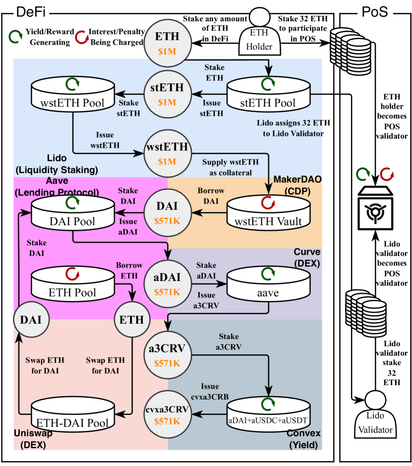
Figure 1. Ether staking and defi composability. The amounts in orange represent the value of tokens deposited or issued. This figure compares the pos staking versus complicated defi staking operations for optimizing rewards with $1 million worth of ETH.

defi is an ecosystem of (defi) protocols operating autonomously through smart contracts run on blockchains. defi protocols are decentralized applications with financial utilities. Many defi protocols, such as asset exchanges and lending platforms, draw inspiration from and mirror traditional centralized finance systems (Xu et al., 2023; Werner et al., 2022; Qin et al., 2021). For our study, we select Lido, MakerDAO, Aave V2, Uniswap V2, Curve, and Convex (see Figure 1). These protocols have the highest tvl and, as of today, represent approximately the 68% of the total tvl  (DefiLlama, 2023). These six protocols can be classified into plf and non-plf.

2.2.1. plf

Protocols for Loanable Funds (plf) are defi protocol that allow users to supply and borrow cryptocurrency under overcollaterization mechanism. The overcollaterization mechanism in PLF necessitates users to pledge increased collateral to borrow a reduced amount of debt, capped at a maximum dollar value equal to the ltv times the debt value. This mechanism ensures the overall solvency of the platform. If a user’s account collateral-to-debt ratio falls below one, the liquidation may be triggered, resulting in a fixed portion of the collateral being wiped out (Qin et al., 2021; MakerDAO, 2022a; Aave, 2022, 2023). In certain plf, as the health ratio drops to various thresholds, the proportion of liquidated collateral varies. In the case of Aave V3, there are two thresholds for liquidation. If the account’s collateral-to-debt ratio is below 1, half of the collateral can be liquidated in a single liquidation. If the ratio drops below 0.95, the entire collateral can be liquidated in a single process (Aave, 2023). plf includes cdp such as MakerDAO (orange block in Figure 1) and lending protocols (purple block). Unlike lending protocols, which allow borrowing of any cryptocurrency, users in cdp can only generate noncustodial stablecoins (CoinMarketCap, 2024). The collateralization model in DeFi’s CDP mirrors a tranche system, where stablecoins represent senior debt and users resemble buyers of the junior tranche in a CDO, as seen in TraFi (Klages-Mundt and Minca, 2022). Stablecoins are a cryptocurrency designed to offer the stability of money to function effectively, aiming to provide price stability relative to a specific reference point, often the USD (Moin et al., 2020).

2.2.2. Non-plf

Applying the method of exclusion, liquidity staking, dex, and yield aggregator fall into the category of non-PLF. Liquidity staking protocols allow users to earn rewards by staking any amount of tokens, while also offering a tradable and liquid receipt for their staked position. The liquidity staking protocol Lido (blue block in Figure 1) accepts any amount of ETH from ETH holders, and in exchange issues liquid receipt tokens (stETH and wstETH) that can be further used in other defi protocol. At the same time, Lido allocates ETH to selected knowledgeable Lido validators in order for them to participate in block attestation in the Ethereum blockchain. Rewards and penalties for block attestation are distributed among staking users, the Lido protocol, and Lido validators. dex such as Uniswap (purple block) and Curve (dark blue) are the defi protocol that allows users to provide liquidity and swap assets (Xu et al., 2023). Yield platforms such as Convex (grey block) are protocols that reward users for staking or providing liquidity on their platform.

2.2.3. defi token, liquidity pool, and defi composability

defi tokens are cryptocurrencies that provide users access to the defi system. The liquidity pool operates as the functional unit within the defi protocol, operating as a smart contract to facilitate users in supplying, borrowing, or swapping defi tokens. defi composability refers to the capability of multiple defi protocols to seamlessly communicate with each other, enabling defi tokens to be chained and integrated to create new defi tokens and financial services. Incentivizing users to contribute liquidity to defi protocols and sustain the functionality of liquidity pools, many protocols provide interest rewards to users staking tokens in these pools. In contrast to pos mentioned in §2.1 where validators cannot utilize locked eth, several defi protocols allow lp to get receipt tokens (e.g. wstETH from Lido in Figure 1) which holds the same notional value of the locked tokens (e.g. stETH staked in Lido). To increase liquidity and achieve other functionality, users can take these new tokens and stake them into other protocols (e.g. MakerDAO). Given the additivity of interest and composability across different protocols, defi users commonly repeat this process multiple times among several protocols to maximize rewards, as depicted in Figure 1. Additionally, defi staking has the advantage of not demanding a minimum deposit or block attestation knowledge compared to pos, making it more appealing for user participation.

2.2.4. defi protocol metrics, double counting, and defi tracing website

To assess the size and popularity of defi protocols, metrics such as tvl, protocol revenue, and protocol users are utilized, with tvl being the most influential and widely used. However, the tvl calculation method faces the known problem of double counting (Chandler, 2020). DeFiLlama (one the few tracing services which aggregates tokens breakdown of almost all defi protocols to compute the tvl) tries to accounts for double counting by excluding protocols categorized under liquidity staking or those feeding tokens into other protocols. DeFiLlama has the “double count” toggle in its tvl dashboard to let users decide whether to filter out the double counting by removing the tvl of protocols that deposit into another protocol from the total tvl of single chain or all chains, as shown in Figure 2. As we will show in §3.3, this approach is both rudimentary and imprecise.

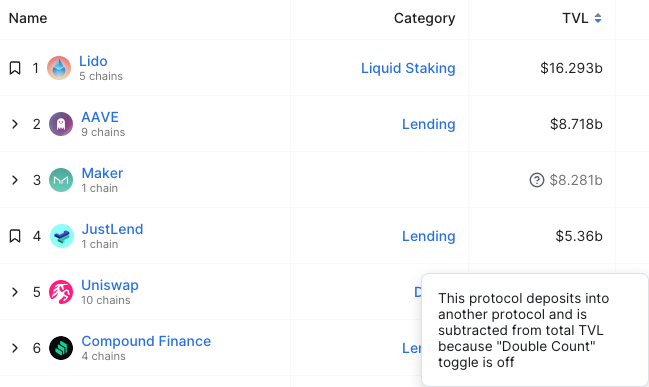
Figure 2. DeFiLlama’s tvl dashboard after activating the double count toggle. When a user activates the double count toggle, protocols that deposit into another protocol will be excluded from the total tvl calculation, and their tvl numbers will be displayed in grey.

2.3. Total Value Locked (TVL)

According to (Binance Academy, 2023; Gogol et al., 2023), we offer the following definition along with a mathematical expression (cf. Equation 1) for the term tvl.

Definition 0 (Total Value Locked).

Total Value Locked is defined as the total value of assets staked by users in a defi protocol or defi ecosystem at a specific moment.

(1) $$TVL_{t}=\sum_{i\in\mathcal{I}_{t}}TVL_{i,t}=\sum_{i\in\mathcal{I}_{t}}\sum_{c\in\mathcal{T}^{i}_{t}}p_{c,t}q^{i}_{c,t}$$

where: $TVL_{t}$ is the total tvl of the defi ecosystem at time $t$; $\mathcal{I}_{t}$ and $\mathcal{T}^{i}_{t}$ are respectively the set of all defi protocols at time $t$ and the set of all tokens in protocol $i$ at time $t$; $TVL_{i,t}$ is the tvl of protocol $i$ at time $t$; $p_{c,t}$ is the dollar price of token $c$ at time $t$; and $q^{i}_{c,t}$ is the quantity of the token $c$ locked in the protocol $i$ at time $t$.

As shown in Table 1, the disclosure of tvl counting methodologies is currently inconsistent across the defi data providers. Each of them offers varying levels of disclosure about their methodologies, with often inconsistent practices among them. Furthermore, only two of them attempt to tackle the issue of double counting. In Figure 1, the TVL is the sum of all orange numbers, totaling 4.7474 million—4.7474 times the initial ETH value deposited.

Table 1. Survey of defi tracing websites with a focus on protocols coverage and tvl-related information disclosure as of 1 March 2024. (●: disclosure, ○: no disclosure)

defi Tracing Website	Protocols Coverage	TVL-related Information
	Number	tvl Presented	Overall Methodology	Protocol-specific Methodology	Toke Price Sources	Constituent Protocols	Code	Double Counting Solution
(DeFiLlama, 2023)	3,570	●	●	●	●	●	●	●
(L2BEAT, 2023)	47	●	●	○	○	●	●	○
(DappRadar, 2022)	4,126	●	○	○	○	●	○	○
(Stelareum, 2023)	309	●	○	○	○	●	○	○
(DeFi Pulse, 2022)	N/A	○	●	○	○	○	○	●

3. TVL Double Counting Analysis

In this section, we explain the double counting problem using a balance-sheet approach. A balance sheet provides a concise overview of an entity’s assets, liabilities, and equities. We apply this traditional accounting framework to defi platforms.

3.1. Balance Sheet of DeFi Protocols

For each specific protocol, we use a balance-sheet approach to consolidate double-entry bookkeeping and describe its financial condition. The aggregate value locked can be regarded as a significant element on the asset side of a defi protocol’s balance sheet (Deloitte, 2023a). In the context of a defi system, we apply the principles of consolidated balance sheets to depict its financial status on an aggregated basis. By leveraging the principle of non-duplication used in consolidated balance sheet accounting (whereby, accounting entries that are recorded as assets in one company and as liabilities in another are eliminated, before aggregating all remaining items) (Deloitte, 2023b), we can effectively eliminate instances of double counting within a defi system.

3.2. The Anatomy of Double Counting Problem

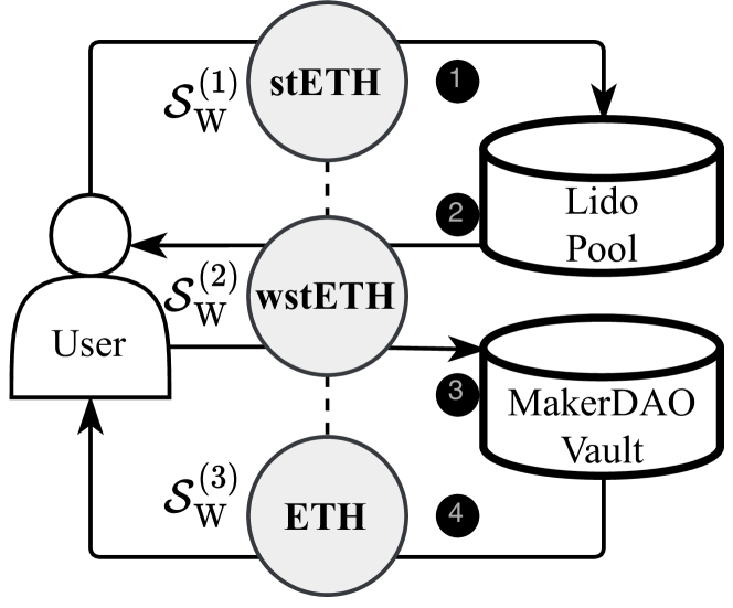
(a) Wrapping in defi.

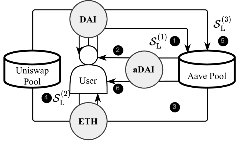
(b) Leveraging in defi.

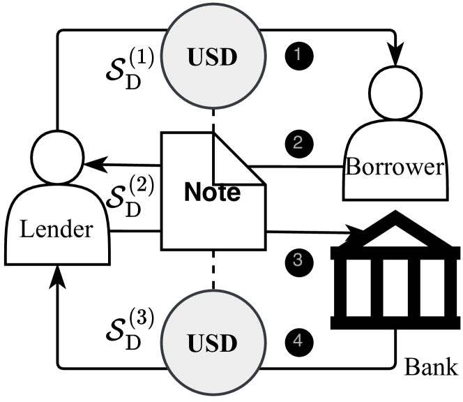
(c) Hypothecation in TradFi.

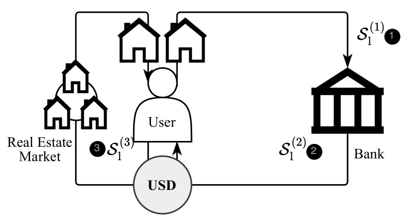
(d) Leveraging in TradFi.

Figure 3. Two common operations of DeFi composability and their corresponding trafi analogies. The process of wrapping in defi, as illustrated in 3(a), mirrors the hypothecation process in trafi, as shown in 3(c). Both defi and trafi involve leveraging processes, depicted in 3(b) and 3(d), respectively. The black circle (●) with a white number indicates the step.

Table 2. Protocol-perspective balance sheets and dynamics of TVL of the wrapping scenario. We highlight the tvl and value locked in red.

(a) Balance sheet of Lido.

	$\mathcal{S}^{(1)}_{\textnormal{W}}$	$\mathcal{S}^{(2)}_{\textnormal{W}}$
Assets	$000	$000
Value Locked - stETH	1,000	1,000
Total Assets	1,000	1,000
Liabilities	$000	$000
Payables - wstETH	1,000	1,000
Total Liabilities	1,000	1,000

(b) Balance sheet of MakerDAO.

	$\mathcal{S}^{(1)}_{\textnormal{W}}$	$\mathcal{S}^{(2)}_{\textnormal{W}}$
Assets	$000	$000
Value Locked - wstETH	-	1,000
Receivables - DAI	-	571
Total Assets	-	$1,571
Liabilities	$000	$000
Payables - wstETH	-	1,000
New Money - DAI	-	571
Total Liabilities	-	1,571

(c) Dynamics of TVL.

	$\mathcal{S}^{(1)}_{\textnormal{W}}$	$\mathcal{S}^{(2)}_{\textnormal{W}}$
	$000	$000
Total Value Locked	1,000	2,000

(d) Consolidated balance sheet of Lido and MakerDAO.

	$\mathcal{S}^{(1)}_{\textnormal{W}}$	$\mathcal{S}^{(2)}_{\textnormal{W}}$
Assets	$000	$000
Value Locked	1,000	1,000
Receivables	-	571
Total Assets	1,000	1,571
Liabilities	$000	$000
Payables	1,000	1,571
Total Liabilities	1,000	1,571

Double counting problem occurs when the value locked in multiple protocols within a defi system is double-counted in the tvl calculation due to composability. The composability enables defi users to achieve sophisticated operations within the defi system (c.f. Figure 1), making the double counting problem non-trivial. For illustration purpose, we describe two common operations that lead to double counting.

3.2.1. Wrapping

3(a) depicts a scenario where an investor initially supplies $1m in stETH to Lido (step 1), which is then converted into $1m of wstETH (step 2). Subsequently, the investor deposits this wstETH into MakerDAO (step 3) and borrows up to $571k in DAI (step 4), based on the tvl of the wstETH low fee vault at the time of this paper. The financial flows generated by the wrapping in defi can be related to the rehypothecation process in trafi, illustrated in 3(c). The promissory hypothecation enables lenders who provide loans to borrowers (step 1) and issue a promissory note (step 2) to pledge the promissory note (step 3) and borrow money from the bank (step 4) (Andolfatto et al., 2017).

Table 2 shows the balance sheets of Lido and MakerDAO, and the consolidated balance sheet of the defi system consists of Lido and MakerDAO. In $\mathcal{S}^{(1)}_{\textnormal{{W}}}$, the value of the DeFi system is $1m, where $\mathcal{S}$ represents a NCB stablecoin (see See Table 4 for a comprehensive list of notations). However, if we deposit the receipt token wstETH from Lido into MakerDAO to issue another receipt token DAI, the tvl will be $2m under the traditional TVL measurement. The balance sheets are expanded and the tvl is double-counted due to the existence of wstETH. In the consolidated balance sheet, the tvl is adjusted to $1m after eliminating the value associated with the wstETH.

3.2.2. Leveraging

Table 3. Protocol-perspective balance sheets and dynamics of TVL of the leveraging scenario. We highlight the tvl in red.

(a) Balance sheet of Aave.

	$\mathcal{S}^{(1)}_{\textnormal{L}}$	$\mathcal{S}^{(3)}_{\textnormal{L}}$
Assets	$000	$000
Value Locked - DAI	2,000	2,900
Receivables - dETH	900	900
Total Assets	2,900	3,800
Liabilities	$000	$000
Payables - aDAI	2,000	2,900
Payables - aETH	900	900
Total Liabilities	2,000	3,800

(b) Balance sheet of Uniswap.

	$\mathcal{S}^{(1)}_{\textnormal{L}}$	$\mathcal{S}^{(3)}_{\textnormal{L}}$
Assets	$000	$000
Value Locked - ETH	1,800	900
Value Locked - DAI	1,800	2,700
Total Assets	3,600	3,600
Liabilities	$000	$000
Payables - ETH-DAI-LP	3,600	3,600
Total Liabilities	3,600	3,600

(c) Dynamics of TVL.

	$\mathcal{S}^{(1)}_{\textnormal{L}}$	$\mathcal{S}^{(3)}_{\textnormal{L}}$
	$000	$000
Total Value Locked	5,600	6,500

(d) Consolidated balance sheet of Aave and Uniswap.

	$\mathcal{S}^{(1)}_{\textnormal{L}}$	$\mathcal{S}^{(3)}_{\textnormal{L}}$
Assets	$000	$000
Value Locked	5,600	5,600
Total Assets	5,600	5,600
Liabilities	$000	$000
Payables	5,600	5,600
Total Liabilities	5,600	5,600

As illustrated in 3(d), the leveraging operation in defi can be related to the leveraging process in trafi. In trafi, the investor can use her house as collateral (step 1) to borrow cash (step 2) and then use cash to buy another house (step 3). In the scenario of 3(b), we assume that liquidity providers have already supplied $900k ETH to Aave and $1.8m ETH along with $1.8m DAI to Uniswap to facilitate swaps and borrowing. Initially, Aave has $900k ETH in assets and $900k worth of aETH in liabilities, while Uniswap holds $1.8m ETH and $1.8m DAI in assets and $1.8m worth of ETH-DAI LP tokens in liabilities. An investor provides $2m DAI (step 1) as collateral to borrow $900k eth (step 3) in Aave, swaps the borrowed $900k eth to $900k DAI (step 4) in Uniswap, and then deposits $900k DAI (step 5) from Uniswap in the Aave to issue the receipt token aDAI (step 6).

Table 3 shows the balance sheets of Aave and Uniswap, and the consolidated balance sheet of the defi system consisting of Aave and Uniswap. In $\mathcal{S}^{(1)}_{\textnormal{L}}$, the value of the DeFi system is $5.6m. However, if the user borrows $900k eth, swaps the eth into DAI, and deposits the DAI into Aave, the tvl will be $6.5m under the traditional tvl measurement. This tvl is also double-counted because it includes DAI. In the consolidated balance sheet, the tvl is adjusted to $5.6m after eliminating the value associated with DAI.

3.3. Limitations in Existing Methodologies Addressing Double Counting

Some defi tracking websites strive to mitigate the issue of double counting, yet they may not be able to eradicate it entirely. The methodology put forward by DeFiLlama, as elaborated in §2.2.4, encounters limitations due to the varying degrees of double counting across different protocols. Thus, simply excluding a particular category of protocols does not suffice to address the problem of double counting comprehensively. This is further illustrated through the example of 3(a), highlighting MakerDAO and Aave, where double counting is evidenced through a balance-sheet analysis, as shown in Table 2. Despite we show the occurrence of double counting within Aave, DeFiLlama accounts for Aave’s tvl (see Figure 2).

4. Enhanced measurement framework

In the following section, we formalize the tvl to show the risk under the traditional tvl framework and introduce our new measurement framework called tvr to accurately assess the value within the defi ecosystem.

4.1. defi Token Classification

To formalize tvl and derive tvr, we initially classify defi tokens $\mathcal{U}$ into plain tokens $\mathcal{F}$ and derivative tokens $\mathcal{F}^{\complement}$, which can be represented as $\mathcal{U}=\mathcal{F}\cup\mathcal{F}^{\complement}$. See Table 4 for a comprehensive list of notations. We provide the following definitions for the plain and underlying tokens:

Table 4. Mathematical notations in formalization.

Notation	Definition
defi token classification
$\mathcal{U}$	Set of staked defi tokens.
$\mathcal{F}$	Set of plain tokens
$\mathcal{F}^{\complement}$	Set of derivative tokens
$\mathcal{G}$	Set of governance tokens such as MKR
$\mathcal{N}$	Set of native tokens such as eth
$\mathcal{S}$	Set of ncb stablecoins such as USDT
$\mathcal{C}$	Set of crypto-backed stablecoins
tvl formalization
$TVL_{t}$	tvl of a defi system at time $t$
$TVL_{i,t}$	tvl of a defi protocol $i$ at time $t$
$\mathcal{I}_{t}$	Set of defi protocols at time $t$
$\mathcal{P}_{t}$	Set of plf at time $t$
$\mathcal{P}^{\complement}_{t}$	Set of non-plf at time $t$
$\mathcal{T}_{i,t}$	Set of token staked in protocol $i$ at time $t$
$p_{i,t}$	Price of token $i$ at time $t$
$q_{i,t}$	Quantity of token $i$ staked in the defi system at time $t$
Endogenous derivative token price formalization
$d$	Derivative token $d$; $d\in\mathcal{F}^{\complement}$
$u$	Underlying token $u$ of derivative token $d$
$\bar{u}$	Ultimate underlying token $\bar{u}$ of derivative token $d$
$\mathcal{L}_{d}$	Set of the underlying tokens of derivative token $d$
$\beta_{u,t}$	The ratio between underlying token $u$ quantity and derivative token $d$ quantity
$\epsilon_{d,t}$	Short-term depegging of derivative token $d$ price due to secondary market’s demand and supply dynamics at time $t$
$\rho_{d,t}$	The pegged value of crypto-backed stablecoin $d$ at time $t$ set by the cdp
$\Gamma_{t}$	The ratio of total collateral value to total debt value in a cdp at time $t$
Endogenous token quantity in plf formalization
$\delta$	Close factor for a specific threshold in a plf, the proportion of collateral wiped out in the liquidation
$\psi$	Threshold for the health factor subjected to different close factors
$\alpha$	The liquidation threshold for a collateral, a percentage at which a position is defined as undercollateralized
$h$	The health ratio computed from the plf user’s collateral value in USD multiplied by the current liquidation threshold $\alpha_{c,t}$ for each of the user’s outstanding assets $c$ at time $t$, divided by the user’s borrow value in USD
$H$	The profitability ratio of an account in a liquidation, computed from the total collateral value in USD divided by the total debt value in USD
$\mathcal{D}$	Set of token borrowed
tvr formalization
$P_{a,t}$	Total payables in the balance sheet of account $a$ at time $t$
$R_{a,t}$	Total receivables in the balance sheet of account $a$ at time $t$
Money multiplier
$M_{t}^{DeFi}$	defi money multiplier computed from tvl divided by tvr
$M_{t}^{TradFi}$	trafi money multiplier computed from M2 divided by M0
$CPI_{t}$	Sticky price consumer price index less food and energy at time $t$
$FFER_{t}$	Federal fund effective rate at time $t$
$S\&P_{t}$	S&P Cryptocurrency Broad Digital Market Index at time $t$
$Gas_{t}$	Ethereum gas price at time $t$
$ETH_{t}$	Ether price at time $t$

Definition 0 (Plain Token).

A defi token without underlying tokens.

Definition 0 (Derivative Token).

A defi receipt token or iou token generated in a given ratio by locking a designated quantity of its underlying tokens into the smart contract of the protocol to represent the ownership of underlying tokens for future redemption.

In the example used in Figure 1, eth is a plain token that is initially deposited in the system and has no underlying token. Instead, other tokens (stETH, wstETH, DAI, aDAI, a3CRV, and cvxa3CRV) are derivative tokens with underlying tokens.

According to Definition 4.1, we can further classify plain tokens into governance tokens $\mathcal{G}$, native tokens $\mathcal{N}$, and ncb tokens $\mathcal{S}$, which can be expressed as $\mathcal{F}=\mathcal{G}\cup\mathcal{N}\cup\mathcal{S}$. Native tokens, encompassing both layer 1 and layer 2 tokens, along with governance tokens, serve as representative units of value within the blockchain and defi projects and have no underlying token, respectively (CoinMarketCap, 2023a, b, c). ncb stablecoins refer to stablecoins that are not backed by other cryptocurrencies.

4.2. Formalizing TVL

4.2.1. tvl formula from the classification

Based on the classification of derivative tokens and plain tokens in §4.1, we can compute the tvl by summing the total value of plain tokens and derivative tokens locked in the system:

(2) $$TVL_{t}=\sum_{i\in\mathcal{I}_{t}}(\underbrace{\sum_{f\in\mathcal{F}_{t}\cap\mathcal{T}_{i,t}}p_{f,t}\cdot q_{f,t}}_{\textnormal{Plain Tokens}}+\underbrace{\sum_{f^{\prime}\in\mathcal{F}^{\complement}_{t}\cap\mathcal{T}_{i,t}}p_{f^{\prime},t}\cdot q_{f^{\prime},t}}_{\textnormal{Derivative Tokens}})$$

4.2.2. Endogenous derivative token price

Derivative tokens have endogenous prices determined by the underlying token prices. According to Definition 4.2, the relationship between the quantity of issued derivative tokens and their locked underlying tokens is defined by a specific ratio. The price of the derivative token is also pegged in a specified ratio, with fluctuations influenced by the secondary market’s demand and supply dynamics.

For derivative tokens that are not crypto-backed stablecoins generated by the cdp, the following relationship exists between the price of the derivative token and the price of all its underlying tokens:

(3) $$p_{d,t}(p_{1,t},p_{2,t},\ldots,p_{\bar{u},t})=\sum_{u\in\mathcal{L}_{d}}\beta_{u,t}\cdot p_{u,t}+\epsilon_{d,t}$$

where $d\in\{x|x\in\mathcal{F}^{\complement},x\notin\mathcal{C}\}$. The temporary depegging $\epsilon_{d,t}$ is exogenous, being associated with the token’s supply and demand dynamics as well as liquidity factors. For example, stETH depegged in 2022 due to the selling pressure from Celsius and market illiquidity (Medium, 2022). For crypto-backed stablecoins generated by the cdp, the relationship is different due to the overcollaterization mechanism. The overcollaterization mechanism requires that cdp users should keep the collateral value higher than the debt value to a certain extent, ensuring the overall solvency of the system. Otherwise, the liquidation of the user account will be triggered, wiping out the user’s collateral. The relationship between the crypto-backed stablecoin and its underlying tokens is as follows:

(4) $$\begin{split}p_{d,t}(p_{1,t},p_{2,t},\ldots,p_{\bar{u},t})&=\begin{cases}\rho_{d,t}+\epsilon_{d,t}&\Gamma_{t}\geq 1\\ &\\ \frac{\displaystyle\sum_{a\in\mathcal{A}}\sum_{u\in\mathcal{T}_{a}}p_{u,t}q_{u,t}}{\displaystyle\sum_{a\in\mathcal{A}}q_{d,t}}+\epsilon_{s,t}&\Gamma_{t}<1\\ \end{cases}\\ &\\ \Gamma_{t}&=\frac{\displaystyle\sum_{a\in\mathcal{A}}\sum_{u\in\mathcal{T}_{a}}p_{u,t}q_{u,t}}{\displaystyle\sum_{a\in\mathcal{A}}\rho_{d,t}q_{d,t}}\end{split}$$

where $d\in\mathcal{C}$. Appendix C shows a detailed explanation of the derivative token pegging mechanism that supports Equation 3 and Equation 4.

defi composability allows the underlying token of a derivative token to serve as the derivative token of another token, as illustrated in Figure 1 and 3(a). We can derive the derivative token price function in terms of its ultimate underlying token, which belongs to the category of plain tokens:

(5) $$\begin{split}&p_{d,t}(p_{1,t},p_{2,t},\ldots,p_{\bar{u},t})=\\ &\left[p_{d,t}\circ p_{d_{1},t}\ldots\circ p_{d_{n},t}\right](p_{1,t},p_{2,t},\ldots,p_{\bar{u},t})\end{split}$$

where $\bar{u}\in\mathcal{F}$ and $\circ$ is the function composition operator.

4.2.3. Endogenous token quantity in plf

Tokens staked in a plf, including cdp such as MakerDAO or lending protocols such as Aave, have a token quantity determined by the token price due to the liquidation mechanism. The quantity of tokens staked in a plf is equal to the summation of the quantity of this token across all accounts. A drop in collateral price results in a reduction of the account’s health ratio, leading to different scenarios: (1) When the health ratio of an account, denoted as $h_{c,t}$, is greater than or equal to 1, the account is deemed safe, and the quantity of collateral in the account remains unchanged, represented by $q_{c,t}$. (2) When the health ratio of an account $h_{c,t}$ falls below 1, the user may face liquidation, prompting the smart contract to transfer varying proportions of collateral $q_{c,t}\delta_{n}$ and sell it off. Additionally, when the profitability ratio of an account, represented by $H_{c,t}$, is greater than or equal to 1, it indicates that the total collateral value is sufficient to cover the total debt value. In this scenario, the liquidation is deemed profitable for liquidators, leading to a successful liquidation. As stated in §2.2.1, health ratios $h_{c,t}$ falling below distinct thresholds $\psi_{n}$ will result in different proportions $\delta_{n}$ of collateral being subject to liquidation. (3) If the profitability ratio of an account, denoted as $H_{c,t}$, is less than 1, the liquidation is considered unprofitable for liquidators, rendering the liquidation unviable and the quantity of collateral in the account unchanged, represented by $q_{c,t}$. For plain tokens staked in the plf, the token quantity can be expressed in Equation 6.

(6) $$\footnotesize\begin{split}q_{c,t}(p_{c,t})&=\sum_{a\in\mathcal{A}}\begin{cases}q_{c,t}&h_{c,t}\geq 1\;\textrm{or}\;H_{c,t}<1\\ q_{c,t}\cdot\left[1-\delta_{0}\right]&\psi_{1}\leq h_{c,t}<1\;\textrm{and}\;H_{c,t}\geq 1\\ q_{c,t}\left[1-\delta_{1}\right]&\psi_{2}\leq h_{c,t}<\psi_{1}\;\textrm{and}\;H_{c,t}\geq 1\\ &\vdots\\ q_{c,t}\left[1-\delta_{n-1}\right]&\psi_{n}\leq h_{c,t}<\psi_{n-1}\;\textrm{and}\;H_{c,t}\geq 1\\ q_{c,t}\left[1-\delta_{n}\right]&h_{c,t}<\psi_{n}\;\textrm{and}\;H_{c,t}\geq 1\end{cases}\\ &\\ &h_{c,t}=\frac{\displaystyle\sum_{c\in\mathcal{F}_{t}\cap\mathcal{T}_{a}}\alpha_{c,t}p_{c,t}q_{c,t}}{\displaystyle\sum_{b\in\mathcal{D}_{a}}p_{b,t}q_{b,t}}\quad H_{c,t}=\frac{\displaystyle\sum_{c\in\mathcal{F}_{t}\cap\mathcal{T}_{a}}p_{c,t}q_{c,t}}{\displaystyle\sum_{b\in\mathcal{D}_{a}}p_{b,t}q_{b,t}}\end{split}$$

The quantity of derivative tokens locked in the plf can be influenced by the price of their ultimate underlying tokens due to the endogenous derivative price. When derivative tokens are staked in the plf account as collateral, the health factor $h_{c,t}$ of the account can be expressed as a function of their underlying token prices $h_{c,t}(p_{1,t},p_{2,t},\ldots,p_{\bar{u},t})$ according to §4.2.2. Since the health factor is the condition of Equation 6, the quantity of derivative tokens locked in the plf can also be the function of its ultimate underlying token prices $q_{c,t}(p_{1,t},p_{2,t},\ldots,p_{\bar{u},t})$.

4.2.4. tvl as a function of ultimate underlying tokens price

According to §4.2.2 and §4.2.3, we can further split the tvl into the following four categories: dollar amount of plain tokens in non-plf ($f\in\mathcal{F}_{t}\cap\mathcal{T}_{i,t}$), plain tokens in a plf ($f\in\mathcal{F}^{\complement}_{t}\cap\mathcal{T}_{i,t}$), derivative tokens in non-plf ($f^{\prime}\in\mathcal{F}^{\complement}_{t}\cap\mathcal{T}_{i,t}$), and derivative tokens in a plf ($f^{\prime}\in\mathcal{F}^{\complement}_{t}\cap\mathcal{T}_{i,t}$). Therefore, we can further derive the following function of tvl in terms of ultimate underlying tokens from Equation 2:

(7) $$\footnotesize\begin{split}&TVL_{t}(p_{1,t},p_{2,t},\ldots,p_{\bar{u},t})\\ &=\sum_{i\in\mathcal{P}_{t}^{\complement}}\left[\sum_{f\in\mathcal{F}_{t}\cap\mathcal{T}_{i,t}}p_{f,t}\cdot q_{f,t}+\sum_{f^{\prime}\in\mathcal{F}^{\complement}_{t}\cap\mathcal{T}_{i,t}}p_{f^{\prime},t}(p_{1,t},p_{2,t},\ldots,p_{\bar{u},t})\cdot q_{f^{\prime},t}\right]\\ &+\sum_{i\in\mathcal{P}_{t}}\left[\sum_{f\in\mathcal{F}^{\complement}_{t}\cap\mathcal{T}_{i,t}}p_{f,t}\cdot q_{f,t}(p_{f,t})\right.\\ &\left.+\sum_{f^{\prime}\in\mathcal{F}^{\complement}_{t}\cap\mathcal{T}_{i,t}}p_{f^{\prime},t}(p_{1,t},p_{2,t},\ldots,p_{\bar{u},t})\cdot q_{f^{\prime},t}(p_{1,t},p_{2,t},\ldots,p_{\bar{u},t})\right]\end{split}$$

4.2.5. Metrics inflation and decentralized financial contagion

The existence of derivative tokens not only inflates the actual value locked by defi users but also serves as the channel for the spread of decentralized financial contagion. The value of derivative tokens in Equation 7 represents the market worth of tokens created through the wrapping process illustrated in 3(a), leading to double counting. Furthermore, due to the endogeneity discussed in §4.2.2 and §4.2.3, the value of derivative tokens will also contribute to the tvl decrease, liquidations, and the depegging of crypto-backed stablecoins when the market experiences downturn, amplifying the impact of price declines of their underlying tokens several times over the value of plain tokens and making the tvl sensitive to the change of plain token price.

4.3. Total Value Redeemable (TVR)

To address the double counting problem discussed in §3.2 and avoid incorporating the risk of decentralized financial contagion discussed in §4.2.5, we introduce the metric tvr.

4.3.1. Definition and formalization of tvr

We offer the following definition along with mathematical expressions (cf. Equation 8) for the term tvr:

Definition 0 (Total Value Redeemable).

Total Value Redeemable is defined as the token value that can be ultimately redeemed from a defi protocol or a defi ecosystem.

We can express the tvr of the whole defi ecosystem as follows:

(8) $$\footnotesize\begin{split}TVR_{t}&=\sum_{i\in\mathcal{I}_{t}}TVR_{i,t}=\sum_{i\in\mathcal{I}_{t}}\underbrace{\sum_{f\in\mathcal{F}_{t}\cap\mathcal{T}_{i,t}}p_{f,t}\cdot q_{f,t}}_{\textnormal{Plain Tokens}}\\ &=\sum_{i\in\mathcal{I}_{t}}(\underbrace{\sum_{g\in\mathcal{G}^{i}_{t}}p_{g,t}\cdot q_{g,t}}_{\textnormal{Governance Tokens}}+\underbrace{\sum_{n\in\mathcal{N}^{i}_{t}}p_{n,t}\cdot q_{n,t}}_{\textnormal{Native Tokens}}+\underbrace{\sum_{s\in\mathcal{S}^{i}_{t}}p_{s,t}\cdot q_{s,t}}_{\textnormal{\ac{ncb} Stablecoins}})\end{split}$$

Compared to tvl, tvr removes the derivative token value and only includes the plain token value to eliminate the double counting problem. The exclusion of inflated values also decreases the complexity of the interplay within the defi system, mitigating the high sensitivity of the metric concerning the ultimate underlying tokens.

When evaluating the tvr for an individual protocol, aggregating the total value of plain tokens is not applicable anymore since there is no inter-protocol wrapping illustrated in 3(a) when focusing solely on a single protocol. However, a naive summation of the token value deposited in the protocol, as done in the traditional tvl framework, is also inappropriate. This is because leveraging (see 3(b)) and intra-protocol wrapping (a variant of 3(a)) could also lead to the double counting and inflate the protocol’s tvl as explained in §3.2.

To avoid intra-protocol double counting, we can employ the notations in the account-perspective balance sheet to accurately evaluate the redeemable value of the individual protocol. We chose Lido as the case study to illustrate intra-protocol wrapping and Aave to show leveraging because they represent the largest protocols where these instances of double counting could occur. 5(a) shows the account-perspective balance sheets of the Lido user in the intra-protocol wrapping scenario. In this scenario, a user deposits 1,000 USD eth to receive 1,000 USD in stETH in state $\mathcal{S}^{(2)}_{\textnormal{W}}$. Subsequently, the user deposits 1,000 USD in stETH to generate 1,000 wstETH in state $\mathcal{S}^{(3)}_{\textnormal{W}}$. From the user’s standpoint, irrespective of the frequency of intra-protocol token wrapping, the total value of receivables remains constant at $1 million in this scenario. 5(b) shows the account-perspective balance sheets of the Aave user in the leveraging scenario, as illustrated in 3(b). When users take leverage to expand both protocol’s (see 3(a)) and their account’s balance sheet, the total value of payables indicates the extent to which receivables are inflated, which is $900,000 in the scenario. Calculating the difference between the total value of receivables and the actual receivables helps offset this inflation. Therefore, the tvr of an individual defi protocol $i$ at time $t$ can be expressed as follows:

(9) $$TVR_{i,t}=\underbrace{\sum_{a\in\mathcal{A}}R_{a,t}}_{\textnormal{Total Receivables}}-\underbrace{\sum_{a\in\mathcal{A}}P_{a,t}}_{\textnormal{Total Payables}}$$

Table 5. Account-perspective balance sheets of the Lido user and the Aave user. In the Lido scenario, the user deposits 1,000 USD eth to receive 1,000 USD stETH and further deposits 1,000 USD stETH to generate 1,000 wstETH. The Aave scenario aligns with the process in 3(b). We highlight receivables in green and payables in red.

(a) Lido user.

	$\mathcal{S}^{(2)}_{\textnormal{W}}$	$\mathcal{S}^{(3)}_{\textnormal{W}}$
Assets	$000	$000
Receivables - stETH	1,000	0
Receivables - wstETH	-	1,000
Total Assets	1,000	1,000
Liabilities	$000	$000
Total Liabilities	0	0
Net Positions	$000	$000
Initial Deposit Value - ETH	1,000	1,000
Total Net Positions	1,000	1,000
Total Liabilities and Net Positions	1,000	1,000

(b) Aave user.

	$\mathcal{S}^{(1)}_{\textnormal{L}}$	$\mathcal{S}^{(2)}_{\textnormal{L}}$	$\mathcal{S}^{(3)}_{\textnormal{L}}$
Assets	$000	$000	$000
Cash - DAI	2,000	0	0
Cash - ETH	-	900	0
Receivables - aDAI	-	2,000	2,000
Receivables - aETH	-	-	900
Total Assets	2,000	2,900	2,900
Liabilities	$000	$000	$000
Payables - dETH	-	900	900
Total Liabilities	0	0	0
Net Positions	$000	$000	$000
Initial Deposit Value - DAI	2,000	2,000	2,000
Total Net Positions	2,000	2,000	2,000
Total Liabilities and Net Positions	2,000	2,900	2,900

4.3.2. tvr Algorithm

We propose the algorithm for the tvr measurement framework. To optimize time complexity, we integrate a hash set to filter plain token values among the breakdowns of protocol tokens for tvr calculation. First, we insert all plain tokens into the hash set. Then, we fetch on-chain token breakdowns of all protocols at this moment. Next, we check whether the token is in the hash table. If the token is in the hash table, its value will be added to the tvr.

Algorithm 1 Comparative sensitivity tests for the change in tvl and tvr in terms of the eth price decline

Input: Protocol list $I_{t}$, ETH price decline in percentage $d$, and on-chain data $D$;

Output: $\Delta TVL$, $\Delta TVR$;

1:Extract ETH and its derivative token list $M$ from $D$

2:for all protocol $i$ in protocol list $I_{t}$ do

3:    Extract token-amount $(c_{n,i,t},a_{n,i,t})$ pairs for protocol $i$ from $D$

4:    for all token-amount pair $(c_{n,i,t},a_{n,i,t})$ do

5:        if $c$ is a plain token then

6:           $\Delta TVL\leftarrow\Delta TVL-a_{n}\cdot d$

7:           $\Delta TVR\leftarrow\Delta TVL-a_{n}\cdot d$

8:        else

9:           Calculate the weight $\beta$ in the composition of $c$

10:           $\Delta TVL\leftarrow\Delta TVL-a_{n}\cdot d\cdot\beta$

11:        end if

12:        Update the token dollar amount $a_{t,n}$ after price change

13:    end for

14:    if the protocol is a PLF then

15:        Extract every account in the PLF $i$ from $D$

16:        for all account $a\in\mathcal{A}$ do

17:           if Health ratio is below the liquidation threshold then

18:               $\Delta TVL\leftarrow\Delta TVL-a_{n}\cdot d\cdot\beta$

19:           end if

20:        end for

21:        if the protocol is a CDP then

22:           if Total debt value is greater than total collateral value then

23:               Update crypto-backed stablecoin price after depegging

24:           end if

25:        end if

26:        for all token-amount pair $(c_{n,i,t},a_{n,i,t})$ do

27:           if $c$ is a depeggd crypto-back stablecoins then

28:               $\Delta TVL\leftarrow\Delta TVL-a_{n}\cdot\frac{\textnormal{CDP total collateral}}{\textnormal{CDP total debt}}$

29:           end if

30:        end for

31:    end if

32:end for

5. Data Collection

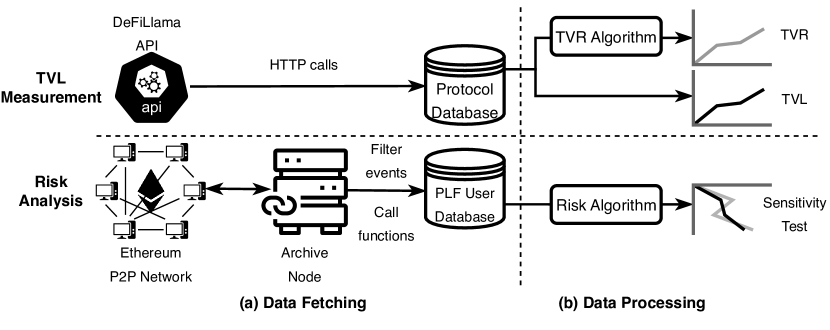
Figure 4. Data pipeline setup overview.

The data pipeline setup is outlined in Figure 4. The data pipeline constitutes two components: tvl measurement and risk analysis. We crawl the tokens breakdown data and adjust tvl ($TVL^{Adj}_{t}$) from 1st January 2021 to 1st March 2024 using DeFiLlama API. DeFiLlama offers the most comprehensive universe of DeFi protocols of all blockchains compared to all other DeFi-tracing websites, as illustrated Table 1. $TVL^{Adj}_{t}$ is DeFiLlama’s improved metric aimed at mitigating the double counting problem and is regarded as flawless in §3.3. We then aggregate the tokens breakdown of each protocol to obtain the tvl per protocol per day ($TVL_{i,t}$). Furthermore, we sum up the $TVL_{i,t}$ across all protocols over time to get the total tvl over time ($TVL_{t}$) and the total tvr ($TVR_{t}$) over time using the tvr filter.

For the risk analysis, we retrieve the data by crawling blockchain states (e.g. MakerDAO vaults data) and blockchain events (e.g. Aave deposit events) from an Ethereum archive node, on a dual AMD Epyc 7F32 with 128 GB DDR4 ECC RAM, 2 $\times$ 240G Intel SSD and 2 $\times$ 16 TB Seagate EXOS in Raid 1 configuration. An Ethereum archive node stores not only the blockchain data but also the chain state at every historical block, supporting efficient historical state query. As of the latest information available, establishing an Ethereum archive node requires disk space ranging from 3 TB to 12 TB. Our sample of risk analysis constitutes six leading defi protocols with the highest tvl within each respective defi protocol category, as shown in Figure 1. Table 6 shows the statistics of accounts in sensitivity tests in MakerDAO and Aave on three representative dates.

Table 6. Statistics of accounts in MakerDAO and Aave on three representative dates.

PLF	Maximum TVL (2021-12-02)	LUNA collapse (2022-05-09)	FTX collapse (2022-11-08)
MakerDAO	27,051	28,220	29,711
Aave	21,336	30,859	47,957

6. Empirical Measurement Results

6.1. tvl, Adjusted tvl, and tvr

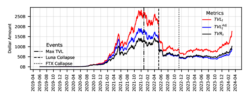
Figure 5. TVL and TVR over time, where the red, blue, and black lines represent the DeFiLlama TVL subjected to double counting, DeFillama adjusted TVL, and TVR.

To apply the tvr framework, we retrieve tvl data from DeFillama from June 1st 2019 to March 1st 2024. DeFiLlama provides raw tvl data subjected to the double counting and adjusted tvl using its methodology to address the double counting problem. We build the tvr from DeFiLlama tvl subjected to double counting using our measurement methodology.

Figure 5 shows the all-chain DeFiLlama tvl subjected to the double counting ($TVL_{t}$), DeFiLlama adjusted tvl ($TVL_{t}^{Adj}$), and tvr ($TVR_{t}$) over time. Our empirical measurement reveals the level of double counting within the DeFi ecosystem, with tvl-tvr discrepancies reaching up to $139.87 bn, and a TVL-TVR ratio of around 2 when the tvl reached its all-time high. Moreover, there is a distinction between DeFiLlama’s adjusted tvl and the tvr due to differences in methodology. Before June 2022, the tvr exceeds DeFiLlama’s adjusted tvl because the token value deposited of removed protocols under DeFiLlama’s methodology is lower than the actual value that needs to be removed within the tvr framework. Conversely, after June 2022, the tvr falls below DeFiLlama’s adjusted tvl because the token value deposited of protocols removed by DeFiLlama is higher than the actual value that needs to be removed within the tvr framework. In both scenarios, the inaccurate valuation of double-counted removals according to DeFiLlama’s methodology is highlighted, as demonstrated in §3.3. However, all three metrics follow a similar trend, encompassing the surge during the defi summer, a period marked by increased investor participation in the defi market, as well as the sharp decline in Luna collapse on May 9, 2022 and FTX collapse on November 8, 2022.

Equation 9 shows the total receivables, total payables, and tvr of Lido and Aave V2 in the Ethereum. The green area represents the value of total receivables, while the red area denotes the value of total payables. The protocol tvl is calculated according to the Equation 9.

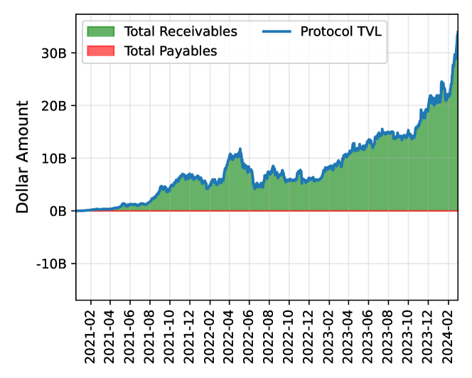
(a) Lido.

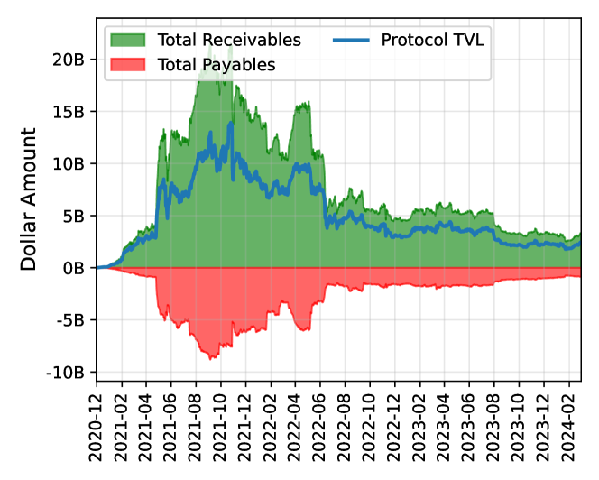
(b) Aave V2.

Figure 6. Total receivables, total payables, and tvr of Lido and Aave V2 in the Ethereum. The green area represents the value of total receivables, the red area denotes the value of total payables, and the blue line illustrates the protocol tvl.

6.2. tvr Decomposition

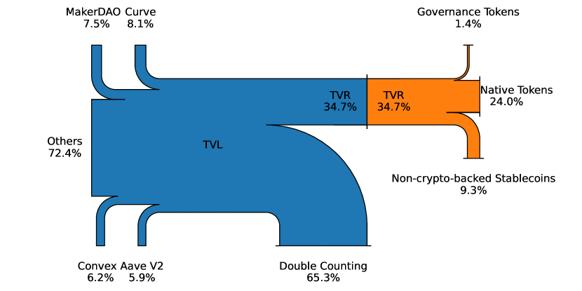
(a) Observation date: 2021-12-02, on which the TVL reaches the maximum value during the sample period.

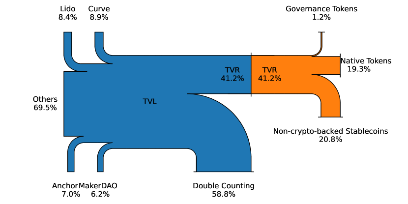
(b) Observation date: 2022-05-09, which is the end of the date of LUNA collapse.

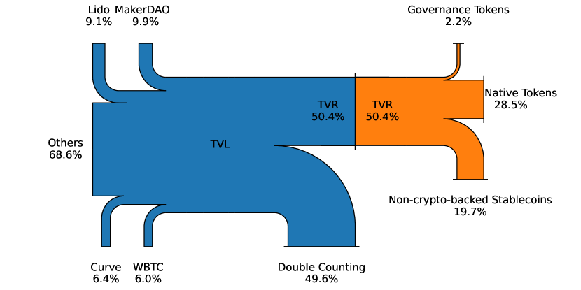
(c) Observation date: 2022-11-08, which is the end of the date of FTX collapse.

Figure 7. Decomposition of tvl. We identify four protocols with the highest tvl and group the remaining protocols under the category of ”Others”. The band width represents the dollar value of tokens. The blue band represents the tvl value, while the orange band represents the tvr value.

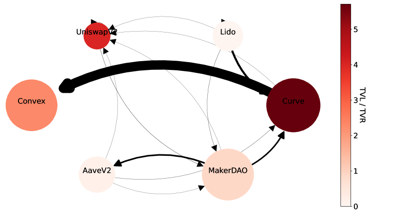
(a) Observation date: 2021-12-02, on which the tvl reaches the maximum value during the sample period.

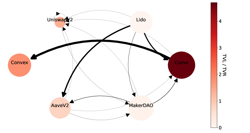
(b) Observation date: 2022-05-09, which is the end of the date of LUNA collapse.

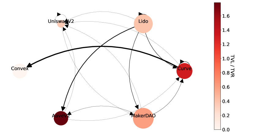
(c) Observation date: 2022-11-08, which is the end of the date of FTX collapse.

Figure 8. Token wrapping network. Node size corresponds to the tvl, edge width represents the dollar amount of tokens generated from the source protocol and staked in the target protocol, and node color reflects the ratio between tvl and tvr. A darker color indicates a higher level of double counting within the defi protocol.

Figure 9 depicts the time series plot of the decomposition of tvr across all chains. We observe that native tokens dominate across all periods, but their percentage decreases before February 2022. The ncb stablecoins surge before October 2020. The percentage of governance tokens experiences a rapid increase before January 2021 and began to decline thereafter. All three types of tokens exhibit stability after February 2022, with ncb tokens and native tokens almost equally distributed. The stability corresponds to the stable period after the LUNA crash and before the FTX collapse in tvl shown by Figure 5. After the FTX collapse, the proportion of native tokens rises, while the proportion of ncb stablecoins declines.

6.3. Risk Analysis

To examine the financial contagion risk derived from the existence of derivative tokens, as discussed in §4.2.5, we conduct comparative sensitivity tests for the change in tvl and tvr in terms of the ETH price decline according to Equation 7. For tractability, we assume that in each liquidation, only one rational liquidator will participate, liquidate the maximum amount of collateral possible, and seize borrowed assets based on their share of the user’s total debt. Leveraging on the data for the six leading defi protocols in Figure 1, these tests are conducted on three representative dates, considering different sets of parameters. In Table 7, we set the default value of certain parameters and discuss the plausibility of selected values for risk-specific parameters via the reference of documentation. We detail how we implement the sensitivity test in Algorithm 1.

Figure 8 shows the double counting that happened among the six leading protocols. We observe that from the point when tvl reaches the maximum value until the collapse of LUNA and FTX, the tvl of protocols, excluding Lido, contracts. Additionally, the overall wrapping effect diminishes. These observations align with the overall defi system dynamics illustrated in Figure 5. Since almost all lp tokens generated from the curve can be staked in convex, the wrapping effect between the Curve and the Convex is significant.

In Figure 10, we show how $\Delta_{TVL}$ and $\Delta_{TVR}$ change with $d_{ETH}$. $\Delta_{TVL}$ curves and $\Delta_{TVR}$ curves with the default parameter setting are plotted in the red lines, which are compared with $\Delta_{TVL}$ curves and $\Delta_{TVR}$ curves with different parameter. Irrespective of parameter values, the $\Delta_{TVL}$ curve is always convex due to the existence of liquidation mechanism in plf and more sensitive to $d_{ETH}$ than the $\Delta_{TVR}$ curve due to the existence of double counting, which aligns with the reasoning in §4.2.5.

Table 7. Default value of parameters.

Parameters	Reference	Value
		Maximum TVL (2021-12-02)	LUNA collapse (2022-05-09)	FTX collapse (2022-11-08)
$p_{ETH}$	CoinGecko	$4075.03	$2249.89	$1334.29
$\delta_{0,AAVE}$	(Aave, 2022)	0.5	0.5	0.5
$\delta_{0,MKR}$	(MakerDAO, 2022a)	1	1	1
$\psi_{1,AAVE}$	(Aave, 2022)	0	0	0

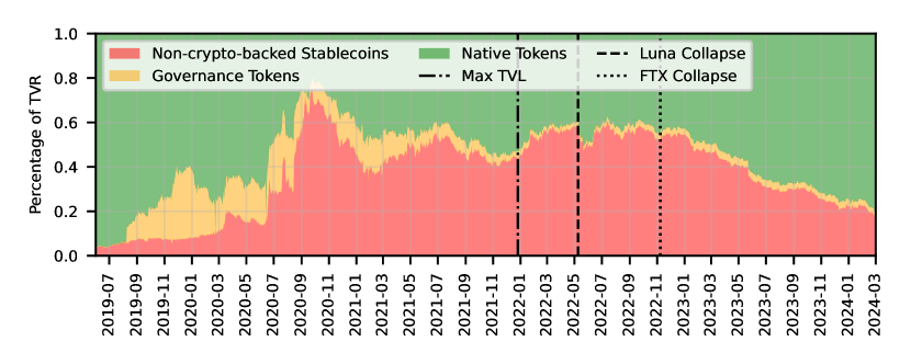
Figure 9. Non-derivative tokens locked in the DeFi before 1st June 2023. The rise of governance tokens and NCB stablecoins weakens the dominance of native tokens before October 2020. Three types of tokens remain stable after July 2022 with native tokens and ncb tokens almost equally distributed. Three vertical lines mark significant events: the peak TVL on December 2, 2021; the collapse of LUNA on May 9, 2022; and the collapse of FTX on November 8, 2022.

Next, we discuss how the value setting of other parameters in Equation 6 affects $\Delta_{TVL}$ and $\Delta_{TVR}$.

1. Close factor $\delta_{0}$: As shown in Figure 10, ceteris paribus, higher $\delta$ leads to greater drop in $\Delta_{TVL}$ and $\Delta_{TVR}$. This is true for both $\delta_{0,AAVE}$ and $\delta_{0,MKR}$. The drop in $\Delta_{TVL}$ under $\delta_{0,MKR}$ is greater than $\delta_{0,AAVE}$ since the MakerDAO’s tvl is higher than Aave V2’s tvl.

2. Liquidation threshold $\psi_{1}$. In Aave V2, $\psi_{1,AAVE}$ corresponds to the close factor $\delta_{1,AAVE}=100\%$, which means that all collateral will be wiped out during the liquidation when the health factor of an account reaches $\psi_{1,AAVE}$. As shown in Figure 10, ceteris paribus, higher $\psi_{1,AAVE}$ leads to earlier drop in $\Delta_{TVL}$ and $\Delta_{TVR}$.

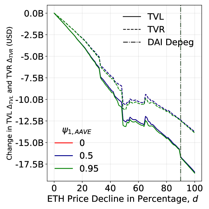
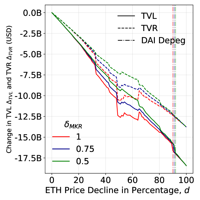
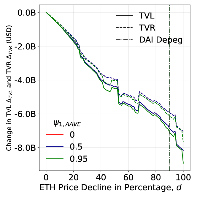
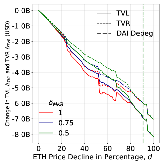
Figure 10. Change in tvl $\Delta_{TVL}$ and tvr $\Delta_{TVR}$ as a function of ETH price decline in percentage $d$ on three representative point with different parameter values. Subfigures within a row represent sensitivity tests conducted under the same snapshot, whereas subfigures within a column display sensitivity tests implemented under three different sets of values for a given parameter.

6.4. DeFi Money Multiplier

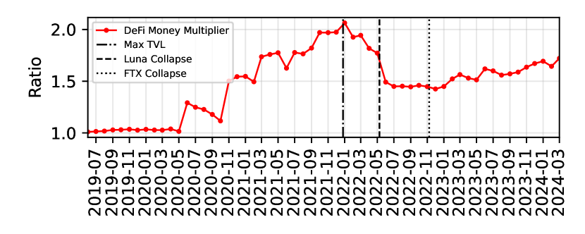
Figure 11. defi money multiplier computed from tvl divided by tvr.

Similar to traditional finance, investors can take leverage in defi. tvr shares similarities with M0, the monetary base in economics, encompassing cash and bank deposits—representing the value directly withdrawable from the system. In comparison, tvl can be likened to M2, which includes M0 plus checking deposits and other short-term deposits.

The M2 to M0 ratio, akin to the traditional “money multiplier”, characterizes the proportion of investor deposits that can be utilized by the bank (FRED, 2023). Drawing a parallel, we can divide tvl by tvr to compute the defi money multiplier:

(10) $$M_{t}^{TraFi}=\frac{TVL_{t}}{TVR_{t}}$$

This ratio mirrors the double counting and wrapping effects within the defi ecosystem, similar to the traditional finance concept of the money multiplier. Figure 11 plots the defi money multiplier.

Table 9 shows the Spearman’s rank correlation coefficients (Spearman, 1904) between the defi money multiplier ($M_{t}^{DeFi}$), key macroeconomic indicators in the US, and representative crypto market indicators. The observed positive correlation between the defi money multiplier and cryptocurrency market indicators such as S&P Cryptocurrency Broad Digital Market Index ($S\&P_{t}$), Ethereum gas price ($Gas_{t}$), and Ether price ($ETH_{t}$) is significant. During bullish periods in the cryptocurrency market, investors exhibit a propensity for increased investment in defi, concurrently opting for leveraged positions. The defi money multiplier is significantly negatively correlated with the trafi money multiplier ($M_{t}^{TradFi}$), showing the substitution effect between the trafi market and defi. As a robustness test, we also calculate Spearman’s rank correlation coefficients (Spearman, 1904) between the natural logarithmic return of these indicators to make variables stationary.

The defi money multiplier, derived from the tvr and tvl, affords a discerning perspective on the prevalence of double counting and the wrapping effect within the decentralized finance defi realm. This metric assumes significance not only for investors navigating the intricacies of defi but also for policymakers seeking to comprehend and address systemic risks within this decentralized financial ecosystem.

Table 8. Spearman’s rank correlation coefficients (Spearman, 1904) between macroeconomic indicators, cryptocurrency market indicators, and defi money multiplier computed from tvl and tvr. *, **, and *** denote the 1%, 5%, and 10% significance levels, respectively.

	Macroeconomic / TradFi indicators				Cryptocurrency / DeFi indicators
	$CPI_{t}$	$FFER_{t}$	$VIX_{t}$	$M_{t}^{TradFi}$	$Gas_{t}$	$ETH_{t}$	$S\&P_{t}$	$M_{t}^{DeFi}$
$CPI_{t}$	1.00∗∗∗	0.71∗∗∗	-0.19	0.06	-0.01	0.28∗	0.07	0.25
$FFER_{t}$	0.71∗∗∗	1.00∗∗∗	-0.43∗∗∗	0.22	-0.33∗	-0.05	-0.22	-0.05
$VIX_{t}$	-0.19	-0.43∗∗∗	1.00∗∗∗	-0.15	0.09	-0.21	-0.19	-0.18
$M_{t}^{TradFi}$	0.06	0.22	-0.15	1.00∗∗∗	-0.36∗∗	-0.66∗∗∗	-0.70∗∗∗	-0.76∗∗∗
$Gas_{t}$	-0.01	-0.33∗	0.09	-0.36∗∗	1.00∗∗∗	0.64∗∗∗	0.65∗∗∗	0.55∗∗∗
$ETH_{t}$	0.28∗	-0.05	-0.21	-0.66∗∗∗	0.64∗∗∗	1.00∗∗∗	0.95∗∗∗	0.91∗∗∗
$S\&P_{t}$	0.07	-0.22	-0.19	-0.70∗∗∗	0.65∗∗∗	0.95∗∗∗	1.00∗∗∗	0.91∗∗∗
$M_{t}^{DeFi}$	0.25	-0.05	-0.18	-0.76∗∗∗	0.55∗∗∗	0.91∗∗∗	0.91∗∗∗	1.00∗∗∗

Table 9. Spearman’s rank correlation coefficients (Spearman, 1904) between the natural logarithmic returns of macroeconomic indicators, cryptocurrency market indicators, and defi money multiplier computed from tvl and tvr. *, **, and *** denote the 1%, 5%, and 10% significance levels, respectively.

	Macroeconomic / TradFi indicators				Cryptocurrency / DeFi indicators
	$\ln\frac{CPI_{t}}{CPI_{t-1}}$	$\ln\frac{FFER_{t}}{FFER_{t-1}}$	$\ln\frac{VIX_{t}}{VIX_{t-1}}$	$\ln\frac{M_{t}^{TradFi}}{M_{t-1}^{TradFi}}$	$\ln\frac{Gas_{t}}{Gas_{t-1}}$	$\ln\frac{ETH_{t}}{ETH_{t-1}}$	$\ln\frac{S\&P_{t}}{S\&P_{t-1}}$	$\ln\frac{M_{t}^{DeFi}}{M_{t-1}^{DeFi}}$
$\ln\frac{CPI_{t}}{CPI_{t-1}}$	1.00∗∗∗	0.30∗	-0.11	0.40∗∗	-0.03	0.06	0.04	-0.01
$\ln\frac{FFER_{t}}{FFER_{t-1}}$	0.30∗	1.00∗∗∗	-0.26	0.69∗∗∗	-0.08	0.09	0.07	-0.16
$\ln\frac{VIX_{t}}{VIX_{t-1}}$	-0.11	-0.26	1.00∗∗∗	-0.25	-0.09	-0.17	-0.25	0.02
$\ln\frac{M_{t}^{TradFi}}{M_{t-1}^{TradFi}}$	0.40∗∗	0.69∗∗∗	-0.25	1.00∗∗∗	-0.04	-0.05	-0.06	-0.08
$\ln\frac{Gas_{t}}{Gas_{t-1}}$	-0.03	-0.08	-0.09	-0.04	1.00∗∗∗	0.56∗∗∗	0.49∗∗∗	0.08
$\ln\frac{ETH_{t}}{ETH_{t-1}}$	0.06	0.09	-0.17	-0.05	0.56∗∗∗	1.00∗∗∗	0.88∗∗∗	0.17
$\ln\frac{S\&P_{t}}{S\&P_{t-1}}$	0.04	0.07	-0.25	-0.06	0.49∗∗∗	0.88∗∗∗	1.00∗∗∗	0.33∗
$\ln\frac{M_{t}^{DeFi}}{M_{t-1}^{DeFi}}$	-0.01	-0.16	0.02	-0.08	0.08	0.17	0.33∗	1.00∗∗∗

7. Related Work

7.1. Total Value Locked

Chiu et al. (2023) leverage on a standard theoretical production-network model to assess the value added and service outputs across various DeFi sectors. Saengchote (2021) examines the flow of a stablecoin between protocols, offering indicative evidence of DeFi yield-chasing behavior, shedding light on the true implications of DeFi total value locked. tvl is a fundamental element in assessing the valuation of defi protocols (Kumar et al., 2022; Şoiman et al., 2023). Stepanova et al. (2021) investigate the evolution of tvl. tvl can work as a valuable tool for monitoring market dynamics and assessing the risk of bubbles in the digital financial landscape (Maouchi et al., 2022).

7.2. Double Counting

Double counting is also common in macroeconomics and the carbon market. The input-output framework that is used to avoid double-counting is well-known in economics (Koopman et al., 2008, 2013, 2014). Double counting, leading to poor emissions accounting, has the potential to undermine carbon markets. Schneider et al. (2019) emphasize the pivotal role of addressing double counting in achieving the goals of the Paris Agreement and identify key elements for a robust resolution that ensures environmental effectiveness and enables cost-effective mitigation.

7.3. Risks in defi

Many researchers study the liquidation risks, financial stability risks, and fragility in the defi lending market (Qin et al., 2021; Chiu et al., 2022; Darlin et al., 2022). Bekemeier (2021) examines the systemic risk in defi. Qin et al. (2022) quantify the on-chain leverage risk in defi. Nadler et al. (2023) introduce a fully decentralized insurance protocol based on smart contracts to allow risk transfer in defi. Tzinas and Zindros (2023) study the principal-agent problem in the context of liquid staking, which leads to unexpected risks due to delegation.

7.4. Financial Contagion

Financial contagion is the transmission of market disturbances, typically negative, across borders on an international scale or between banks domestically (Bavister and Squirrell, 2000). Debates persist regarding the underlying causes of financial contagion. (Longstaff, 2010) empirically investigate the pricing dynamics of subprime asset-backed cdo and their contagion impact on other markets. (Allen and Gale, 2000) and (Lagunoff and Schreft, 2001) investigate financial contagion arising from financial links among financial intermediaries. (Kaminsky and Reinhart, 2000) document that interconnected trade relations and shared exposure to a common creditor can explain previous clusters of crises, including not only the debt crises of the early 1980s and 1990s but also the historical trend of contagion. (Kiyotaki and Moore, 2002), (Kaminsky et al., 2003), (King and Wadhwani, 1990), (Calvo, 2004), and others, outline mechanisms where negative shocks in one market signify the arrival of economic news directly impacting collateral values or cash flows associated with securities in other markets. In this scenario, contagion can be seen as the transmission of information from more-liquid or swiftly price-discovering markets to others. (Vayanos, 2004), (Acharya and Pedersen, 2005), (Longstaff, 2010), and additional researchers suggest that a significant negative shock in one market could lead to an elevation in the risk premium in other markets. In this scenario, contagion arises as adverse returns in the distressed market influence subsequent returns in other markets through a time-varying risk premium.

8. Discussion

Despite the valuable contributions made, this paper acknowledges certain limitations.

8.1. Granularity

One notable area for potential expansion involves extending the concepts of tvr and tvl beyond the protocol level to the smart contract level. Within the defi ecosystem, there exist not only protocols built on smart contracts but also isolated token contracts that could play a role in generating derivative tokens. A direction for future studies could involve broadening the scope of tvl and tvr. Researchers might consider encompassing the aggregation of all defi smart contracts. This approach would provide a more comprehensive understanding of the total value and risk within the defi landscape, offering insights into the broader implications of these metrics.

8.2. Subjectivity

This paper acknowledges the subjective nature of tvr measurement, highlighting the absence of a clear method for automating it. Careful manual processing is essential for distinguishing between plain and derivative tokens. Variation in lists of plain tokens may result in different tvr. Due to resource constraints, this paper opts to retrieve the plain token list from CoinMarketCap rather than label it. Future research could explore automation techniques for distinguishing plain and derivative tokens.

9. Conclusion

This paper empirically analyzes how double counting arises in the traditional tvl framework. We introduce an enhanced measurement framework, the tvr, to evaluate the actual value locked within a defi system and mitigate double counting. By decomposing tvl of all defi protocols and calculating tvr, we find a substantial amount of double counting within the defi system, with a maximum of 182.15 billion with a tvl-tvr ratio around 3. We track the evolution of token composition in tvr over time. Additionally, we uncover the escalating crash risk stemming from double counting within the traditional tvl framework, employing the systems of two prominent protocols. We highlight the pronounced sensitivity of tvl to token prices when double counting exists, showing that tvr is a more stable metric when compared to tvl. We propose the defi money multiplier, drawing parallels with the trafi macroeconomic money multiplier. The defi multiplier utilizes both tvr and tvl to quantify double counting. We document that the defi money multiplier is positively correlated with crypto market indicators and negatively correlated with macroeconomic indicators.

APPENDIX

Appendix A Ethics

This work does not raise any ethical issues

Appendix B DeFi Bookkeeping

We model value transfers of common transactions in defi protocols via the double-entry bookkeeping in the traditional accounting framework. The double-entry booking keeping has two equal journal entries known as debit (Dr.) and credit (Cr.), which represent a transfer of value to and from that account, respectively (Irving, 1912). The credit side should be indented.

Table 10. Journal entries of common transactions in DeFi protocols.

Protocol	Transaction	Definition	Journal Entry	Quantity	Amount	Type	Example Transaction
MakerDAO	Borrowing.	User supplies $q_{T}$ tokens T with dollar price $p_{T}$ as collateral to mint $q_{S}$ stablecoins S with dollar price $p_{S}$.	Dr. Receivables – S Dr. Value Locked – T       Cr. New Money – S       Cr. Payables – T	$q_{S}$ $q_{T}$       $q_{S}$       $q_{T}$	$q_{S}\times p_{S}$ $q_{T}\times p_{T}$       $q_{S}\times p_{S}$       $q_{T}\times p_{T}$	Assets Assets Liabilities Liabilities	0x959…0adb
MakerDAO	Stability fee accrual.	Debt accrues $I_{S}$ when its dollar price is $p_{S}$.	Dr. Receivables – S       Cr. Unrealized Gain – S	$I_{S}$       $I_{S}$	$I_{S}\times p_{S}$       $I_{S}\times p_{S}$	Assets Equities	-
MakerDAO	Repayment and collateral withdrawal.	User repays $q_{S}$ stablecoins S with dollar price $p_{S}$ and withdraws $q_{T}$ collateral T with dollar price $p_{T}$.	Dr. New Money – S Dr. Payables – T       Cr. Receivables – S       Cr. Value Locked – T	$q_{S}$ $q_{T}$       $q_{S}$       $q_{T}$	$q_{S}\times p_{S}$ $q_{T}\times p_{T}$       $q_{S}\times p_{S}$       $q_{T}\times p_{T}$	Liabilities Liabilities Assets Assets	0x284…701e
MakerDAO	Collateral price appreciation.	$q_{T}$ collateral experiences price appreciation $\Delta_{p}$.	Dr. Value Locked – T       Cr. Payables – T	$\Delta_{p}$       $\Delta_{p}$	$q_{T}\times\Delta_{p}$       $q_{T}\times\Delta_{p}$	Assets Liabilities	-
MakerDAO	Collateral price depreciation.	$q_{T}$ collateral experiences price depreciation $\Delta_{p}$.	Dr. Payables – T       Cr. Value Locked – T	$\Delta_{p}$       $\Delta_{p}$	$q_{T}\times\Delta_{p}$       $q_{T}\times\Delta_{p}$	Liabilities Assets	-
MakerDAO	Liquidation penalty.	A liquidation penalty $\delta$ applies to the initial debt and accrual stability fee when the collateral-to-debt ratio of the user’s vault is lower than the liquidation ratio.	Dr. Receivables – $\delta(q_{S}+I_{S})$       Cr. Unrealized Gain – $\delta(q_{S}+I_{S})$	$\delta(q_{S}+I_{S})$       $\delta(q_{S}+I_{S})$	$\delta(q_{S}+I_{S})\times p_{S}$       $\delta(q_{S}+I_{S})\times p_{S}$	Assets Equities	-
MakerDAO	Liquidation settlement.	The liquidator wins in the debt auction, sells $q_{T}$ collateral with dollar price $p_{T}$, and repays debt $q_{S}$, liquidation penalty $\delta(q_{S}+I_{S})$ and stability fee $I_{S}$ with dollar price $p_{S}$ of the liquidated vault.	Dr. New Money – S Dr. Unrealized Gain – S Dr. Payables – T       Cr. Receivables – S       Cr. Value Locked – T	$q_{S}$ $I_{S}+\delta(q_{S}+I_{S})$ $q_{T}$       $(1+\delta)(q_{S}+I_{S})$       $q_{T}$	$q_{S}\times p_{S}$ $(I_{S}+\delta(q_{S}+I_{S}))\times p_{S}$ $q_{T}\times p_{T}$       $(1+\delta)(q_{S}+I_{S})\times p_{S}$       $q_{T}\times p_{T}$	Liabilities Equities Liabilities Assets Assets	0x4d0…cbb4
Aave	Supplying.	User supplies $q_{T}$ tokens T with dollar price $p_{T}$ as collateral to issue $q_{A}$ aToken A with dollar price $p_{A}$	Dr. Value Locked – T       Cr. Payables – A	$q_{T}$       $q_{A}$	$q_{T}\times p_{T}$       $q_{A}\times p_{A}$	Assets Liabilities	0xd49…8a04
Aave	Borrowing.	A user borrows $q_{B}$ tokens B with dollar price $p_{B}$ in a lending protocol to receive $q_{D}$ debt tokens D with dollar price $p_{D}$.	Dr. Receivables – D       Cr. Value Locked – B	$q_{D}$       $q_{B}$	$q_{D}\times p_{D}$       $q_{B}\times p_{B}$	Assets Assets	0xf7d…a661
Aave	Debt interest accrual.	Debt token accrues $I_{D}$ when its dollar price is $p_{D}$, representing debt accruals $I_{B}$ when its dollar price is $p_{B}$	Dr. Receivables – D       Cr. Unrealized Gain – B	$I_{D}$       $I_{B}$	$I_{D}\times p_{D}$       $I_{B}\times p_{B}$	Assets Equities	-
Aave	Repayment.	A user repays $q_{B}$ tokens B with dollar price $p_{B}$ to burn $q_{D}$ debt tokens D with dollar price $p_{D}$.	Dr. Value Locked – B       Cr. Receivables – D	$q_{T}$       $q_{D}$	$q_{T}\times p_{T}$       $q_{D}\times p_{D}$	Assets Assets	0x95e…f410
Aave	Collateral price appreciation.	$q_{T}$ collateral experiences price appreciation $\Delta_{p}$.	Dr. Value Locked – T       Cr. Payables – T	$\Delta_{p}$       $\Delta_{p}$	$q_{T}\times\Delta_{p}$       $q_{T}\times\Delta_{p}$	Assets Liabilities	-
Aave	Collateral price depreciation.	$q_{T}$ collateral experiences price depreciation $\Delta_{p}$.	Dr. Payables – T       Cr. Value Locked – T	$\Delta_{p}$       $\Delta_{p}$	$q_{T}\times\Delta_{p}$       $q_{T}\times\Delta_{p}$	Liabilities Assets	-
Aave	Liquidation settlement.	When the health factor of an Aave user is lower than one, the liquidator will trigger the liquidation. The liquidator repays $\mu(q_{D}+I_{D})$ token B with dollar price $p_{D}$ to receive $\mu(q_{D}+I_{D})(1+\delta)$ collateral token T, where $\mu$ is the close factor and $\delta$ is the liquidation bonus. The accrual interest is realized via minting atoken.	Dr. Value Locked – B Dr. Unrealized Gain – B Dr. Payables – A       Cr. Receivables – D       Cr. Realized Gain – A       Cr. Value Locked – T	$\mu(q_{B}+I_{B})$ $\mu I_{B}$ $\mu(q_{B}+I_{B})(1+\delta)$       $\mu(q_{B}+I_{B})$       $\mu I_{B}$       $\mu(q_{B}+I_{B})(1+\delta)$	$\mu(q_{B}+I_{B})\times p_{B}$ $I_{B}\times p_{B}$ $\mu(q_{B}+I_{B})(1+\delta)\times p_{A}$       $\mu(q_{B}+I_{B})\times p_{B}$       $\mu I_{B}\times p_{B}$       $\mu(q_{B}+I_{B})(1+\delta)\times p_{T}$	Assets Equities Liabilities Assets Equities Assets	0x682…7459

Appendix C Derivative Token Pegging Mechanism

For derivative tokens that are not crypto-backed stablecoins generated by the cdp, In cases where the pegged value of the derivative token deviates from the market value, it becomes subject to the arbitrage processes outlined in Arbitrager’s Strategy 1 for values above the market and Arbitrager’s Strategy 2 for values below the market.

For crypto-backed stablecoins generated by the cdp, the stablecoin value is pegged to the value of fiat currency through two mechanisms if the total debt value $\displaystyle\sum_{a\in\mathcal{A}}\rho_{d,t}q_{d,t}$ is above the total collateral value $\sum\limits_{a\in\mathcal{A}}\sum\limits_{u\in\mathcal{T}_{a}}p_{u,t}q_{u,t}$. Crypto-backed stablecoins utilize cdp User’s Strategies 3 and 4 for pegging. To enhance liquidity and pegging stability, some cdp employ a pool between crypto-backed and non-crypto-backed stablecoins (e.g., MakerDAO’s peg stability module (MakerDAO, 2022b)), which allows swapping between the two stablecoins. This setup enables Arbitrager’s Strategies 1 and 2 to facilitate the pegging. If the total debt value $L$ is below the total collateral value, the crypto-backed stablecoins will depeg, with their price equal to the pegged value times the ratio between the total collateral value and debt value.

Table 11. Derivative token pegging mechanism.

Arbitrager’s Strategy 1  $p_{d,t}^{\prime}<\displaystyle\sum_{u\in\mathcal{L}_{d}}\beta_{u,t}\cdot p_{u,t}+\epsilon_{d,t},\hskip 2.84544ptd\in\{x|x\in\mathcal{F}^{\complement},x\notin\mathcal{C}\}$    or    $p_{d,t}^{\prime}<\rho_{d,t}+\epsilon_{d,t},\hskip 2.84544ptd\in\mathcal{C}$

1: Buy $\lambda$ derivative tokens $d$ at price $p_{d,t}$ from the market using $\lambda\cdot p_{d,t}^{\prime}$ (scalar $\lambda$ depends on the budget).

2: Burn derivative tokens $d$ to redeem all underlying tokens $u\in\mathcal{L}_{d}$ in the given ratio $\beta_{u,t}$ in the liquidity pool.

3: Sell all underlying tokens $d$ to get $\lambda\cdot p_{d,t}$ dollar and increase derivative token price $p_{u,t+1}^{\prime}$.

4: Earn profit $\lambda(p_{d,t}-p_{d,t}^{\prime})$ and repeat steps 1 to 5 until $p_{d,t+1}^{\prime}=p_{d,t+1}$, i.e. $\epsilon_{d,t+1}=0$.

Arbitrager’s Strategy 2  $p_{d,t}^{\prime}>\displaystyle\sum_{u\in\mathcal{L}_{d}}\beta_{u,t}\cdot p_{u,t}+\epsilon_{d,t},\hskip 2.84544ptd\in\{x|x\in\mathcal{F}^{\complement},x\notin\mathcal{C}\}$    or    $p_{d,t}^{\prime}>\rho_{d,t}+\epsilon_{d,t},\hskip 2.84544ptd\in\mathcal{C}$

1: Buy all its underlying tokens $u\in\mathcal{L}_{d}$ in the given ratio $\beta_{u,t}$ from the market using $\lambda\cdot p_{d,t}^{\prime}$ (scalar $\lambda$ depends on the budget).

2: Lock all underlying tokens $u$ in the given ratio $\beta_{u,t}$ to issue $\lambda$ derivative token $d$ in the liquidity pool.

3: Sell $\lambda$ derivative token $d$ to get $\lambda\cdot p_{d,t}$ dollar and reduce derivative token price $p_{u,t+1}^{\prime}$.

4: Earn profit $\lambda(p_{d,t}^{\prime}-p_{d,t})$ and repeat steps 1 to 5 until $p_{d,t+1}^{\prime}=p_{d,t+1}$, i.e. $\epsilon_{d,t+1}=0$.

Vault Owner’s Strategy 1  $p_{d,t}^{\prime}<\begin{cases}\rho_{d,t}+\epsilon_{d,t}&\frac{\sum_{a\in\mathcal{A}}\sum_{u\in\mathcal{T}_{a}}p_{u,t}q_{u,t}}{\sum_{a\in\mathcal{A}}\rho_{d,t}q_{d,t}}\geq 1\\ &\\ \frac{\sum_{a\in\mathcal{A}}\sum_{u\in\mathcal{T}_{a}}p_{u,t}q_{u,t}}{\sum_{a\in\mathcal{A}}q_{d,t}}+\epsilon_{s,t}&\frac{\sum_{a\in\mathcal{A}}\sum_{u\in\mathcal{T}_{a}}p_{u,t}q_{u,t}}{\sum_{a\in\mathcal{A}}\rho_{d,t}q_{d,t}}<1\\ \end{cases}$

1: Buy $q_{d,t}$ crypto-backed stablecoin $d$ at price $p_{d,t}^{\prime}$ from the market, with the total cost being the dollar amount of debt $q_{d,t}p_{d,t}^{\prime}$.

2: Repay $L$ debt to unlock all collateral from the cdp.

3: Save a cost of $q_{d,t}(p_{d,t}-p_{d,t}^{\prime})$ to unlock all collateral and increase crypto-backed stablecoin price by decreasing its supply.

Vault Owner’s Strategy 1  $p_{d,t}^{\prime}>\begin{cases}\rho_{d,t}+\epsilon_{d,t}&\frac{\sum_{a\in\mathcal{A}}\sum_{u\in\mathcal{T}_{a}}p_{u,t}q_{u,t}}{\sum_{a\in\mathcal{A}}\rho_{d,t}q_{d,t}}\geq 1\\ &\\ \frac{\sum_{a\in\mathcal{A}}\sum_{u\in\mathcal{T}_{a}}p_{u,t}q_{u,t}}{\sum_{a\in\mathcal{A}}q_{d,t}}+\epsilon_{s,t}&\frac{\sum_{a\in\mathcal{A}}\sum_{u\in\mathcal{T}_{a}}p_{u,t}q_{u,t}}{\sum_{a\in\mathcal{A}}\rho_{d,t}q_{d,t}}<1\\ \end{cases}$

1: Observe that crypto-backed stablecoin price $p_{d,t}^{\prime}$ in the market is higher than its peg value $p_{d,t}$, i.e. $\epsilon_{d,t}>0$.

2: Supply more collateral to increase the collateral-to-debt ratio to decrease the probability of liquidation.

3: Decrease crypto-backed stablecoin price by increasing its supply.

Appendix D Esoteric Blockchain Analysis

To gain a broader understanding of the double-counting issue, we analyze two esoteric blockchains: Hedera ranked 42nd in tvl and Ultron ranked 21st in tvl. Our findings indicate that blockchains with limited infrastructure feature simpler token-wrapping networks, which leads to less double counting. Additionally, we observe that the DeFiLlama framework addressing the double counting might deflate the true value redeemable of an esoteric blockchain.

D.1. Hedera

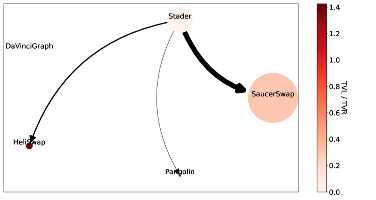
Figure 12. Token wrapping network of Hedera on the observation date: 2024-03-01, which is the end of the sample period. Node size corresponds to the tvl, edge width represents the dollar amount of tokens generated from the source protocol and staked in the target protocol, and node color reflects the ratio between tvl and tvr. A darker color indicates a higher level of double counting within the defi protocol.

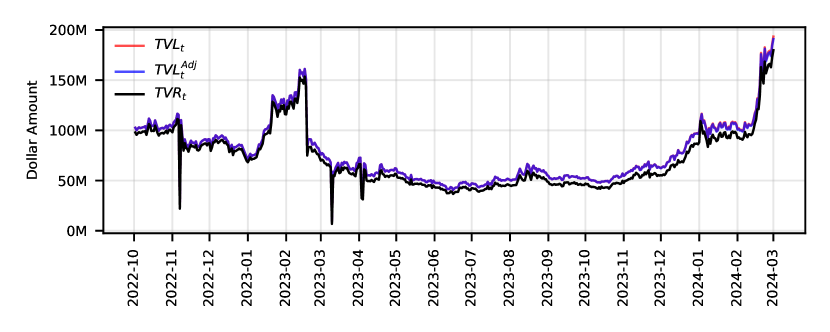
Figure 13. TVL and TVR of Hedera over time, where the red, blue, and black lines represent the DeFiLlama TVL subjected to double counting, DeFillama adjusted TVL, and TVR.

Hedera is a public hashgraph blockchain and governing body tailored to meet the requirements of mainstream markets (Baird et al., 2018). Figure 12 shows the token wrapping network of Hedera at the end of the sample period. Hedera only has eight DeFi protocols, with three projects having zero TVL and being shut down. Among the other six protocols, only one liquidity staking protocol named Stader can generate receipt tokens that can be subsequently deposited into other protocols. Compared to the networks in Ethereum mentioned in §6.3, Hedera has a simpler token-wrapping network, thus experiencing less double counting under the tvl framework. Figure 13 shows the tvl and tvr of Hedera.

D.2. Ultron

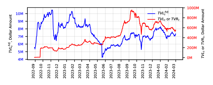
Figure 14. TVL and TVR of Ultron over time, where the red line represents the DeFiLlama TVL subjected to double counting and TVR. The blue line represents the DeFillama-adjusted TVL. The left-hand-side y-axis denotes the dollar amount of DeFillama-adjusted TVL, while the right-hand-side y-axis represents the DeFiLlama TVL subjected to double counting.

Ultron is an esoteric layer 1 blockchain (Ultron, 2023) with three defi protocols in its ecosystem. The Ultron Staking Hub NFT, created by the Ultron Foundation, serves as a digital asset growth instrument allowing users to earn daily apr returns in Ultron native tokens. Each user can mint nft and stake them on the protocol for 5 years with a vesting schedule. All liquidity is securely locked within a staking smart contract and can be claimed at specific timelines. UltronSwap and iZiSwap are two dex on Ultron.

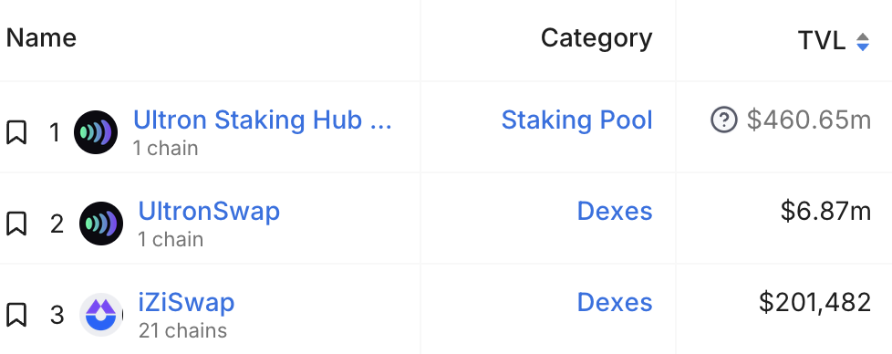
Figure 15. DeFiLlama removes the TVL of the Ultron Staking Hub NFT protocol from Ultron’s TVL excluding double counting, as this protocol falls under the category of protocols that deposit into another protocol.

Ultron does not involve wrapping or leverage. nft minted by Ultron Staking Hub NFT and lp tokens generated by two dex cannot be further deposited into other protocols. Therefore, Ultron is not subject to the double counting problem under the tvr framework. However, DeFiLlama removes the TVL of the Ultron Staking Hub NFT protocol from Ultron’s tvl excluding double counting, as this protocol falls under the category of protocols that deposit into another protocol. DeFiLlama’s methodology is inaccurate as demonstrated in §3.3, making the DeFillama-adjusted TVL of Ultron significantly lower than its tvr as shown in Figure 14.

References

- (1)
- Aave (2022) Aave. 2022. Liquidations - Aave V2. https://docs.aave.com/developers/v/2.0/guides/liquidations#calculating-profitability-vs-gas-cost
- Aave (2023) Aave. 2023. Liquidations - Aave V3. https://docs.aave.com/developers/guides/liquidations
- Acharya and Pedersen (2005) Viral V. Acharya and Lasse Heje Pedersen. 2005. Asset pricing with liquidity risk. Journal of Financial Economics 77, 2 (8 2005), 375–410. https://doi.org/10.1016/J.JFINECO.2004.06.007
- Allen and Gale (2000) Franklin Allen and Douglas Gale. 2000. Financial Contagion. https://doi.org/10.1086/262109 108, 1 (2000), 1–33. https://doi.org/10.1086/262109
- Andolfatto et al. (2017) David Andolfatto, Fernando M. Martin, and Shengxing Zhang. 2017. Rehypothecation and liquidity. European Economic Review 100 (11 2017), 488–505. https://doi.org/10.1016/J.EUROECOREV.2017.09.010
- Baird et al. (2018) Leemon Baird, Mance Harmon, and Paul Madsen. 2018. Hedera: A Public Hashgraph Network & Governing Council. (2018).
- Bavister and Squirrell (2000) Barry D. Bavister and Jayne M. Squirrell. 2000. Contagion: Understanding How It Spreads. The World Bank Research Observer 15, 2 (8 2000), 177–197. https://doi.org/10.1093/WBRO/15.2.177
- Bekemeier (2021) Felix Bekemeier. 2021. Deceptive Assurance? A onceptual View on Systemic Risk in Decentralized Finance (DeFi). ACM International Conference Proceeding Series (12 2021), 76–87. https://doi.org/10.1145/3510487.3510499
- Binance Academy (2023) Binance Academy. 2023. Total Value Locked (TVL). https://academy.binance.com/en/glossary/total-value-locked-tvl
- Calvo (2004) Guillermo A. Calvo. 2004. Contagion in Emerging Markets: When Wall Street is a Carrier. Latin American Economic Crises (2004), 81–91. https://doi.org/10.1057/9781403943859{_}5
- Chandler (2020) Simon Chandler. 2020. DeFi’s ‘Total Value Locked In’ Metric Is A Crooked Mirror. https://cryptonews.com/exclusives/defi-s-total-value-locked-in-metric-is-a-crooked-mirror-7694.htm
- Chiu et al. (2022) Jonathan Chiu, Ozdenoren Emre, Kathy Yuan, and Shengxing Zhang. 2022. On the Inherent Fragility of DeFi Lending. (2022). https://g20.org/wp-content/uploads/2022/02/FSB-Report-on-Assessment-of-Risks-to-Financial-
- Chiu et al. (2023) Jonathan Chiu, Thorsten V. Koeppl, Hanna Yu, and Shengxing Zhang. 2023. Understanding Defi Through the Lens of a Production-Network Model. SSRN Electronic Journal (6 2023). https://doi.org/10.2139/SSRN.4487615
- CoinMarketCap (2023a) CoinMarketCap. 2023a. Top Governance Tokens by Market Capitalization. https://coinmarketcap.com/view/governance/
- CoinMarketCap (2023b) CoinMarketCap. 2023b. Top Layer 1 Tokens by Market Capitalization. https://coinmarketcap.com/view/layer-1/
- CoinMarketCap (2023c) CoinMarketCap. 2023c. Top Layer 2 Tokens by Market Capitalization. https://coinmarketcap.com/view/layer-2/
- CoinMarketCap (2024) CoinMarketCap. 2024. Collateralized Debt Position (CDP) Definition. https://coinmarketcap.com/academy/glossary/collateralized-debt-position-cdp
- DappRadar (2022) DappRadar. 2022. DeFi Rankings. https://docs.dappradar.com/rankings/defi-rankings
- Darlin et al. (2022) Michael Darlin, Georgios Palaiokrassas, and Leandros Tassiulas. 2022. Debt-Financed Collateral and Stability Risks in the DeFi Ecosystem. 2022 4th Conference on Blockchain Research and Applications for Innovative Networks and Services, BRAINS 2022 (2022), 5–12. https://doi.org/10.1109/BRAINS55737.2022.9909090
- DeFi Pulse (2022) DeFi Pulse. 2022. Total Value Locked (TVL). https://docs.defipulse.com/methodology/tvl
- DefiLlama (2023) DefiLlama. 2023. DeFi Dashboard. https://defillama.com/
- DeFiLlama (2023) DeFiLlama. 2023. DefiLlama and our methodology. https://docs.llama.fi/list-your-project/readme
- Deloitte (2023a) Deloitte. 2023a. IAS 1 — Presentation of Financial Statements. https://www.iasplus.com/en/standards/ias/ias1
- Deloitte (2023b) Deloitte. 2023b. IFRS 10 — Consolidated Financial Statements. https://www.iasplus.com/en/standards/ifrs/ifrs10
- ethereum.org (2024) ethereum.org. 2024. Proof-of-stake (PoS). https://ethereum.org/developers/docs/consensus-mechanisms/pos
- FRED (2023) FRED. 2023. The monetary multiplier and bank reserves. https://fredblog.stlouisfed.org/2023/07/the-monetary-multiplier-and-bank-reserves/
- Gogol et al. (2023) Krzysztof Gogol, Christian Killer, Malte Schlosser, Thomas Bocek, and Burkhard Stiller. 2023. SoK: Decentralized Finance (DeFi)-Fundamentals, Taxonomy and Risks. Authorea Preprints (6 2023). https://doi.org/10.22541/AU.168568220.09436681/V1
- Irving (1912) Fisher Irving. 1912. Elementary Principles of Economics. 69 pages.
- Kaminsky and Reinhart (2000) Graciela L. Kaminsky and Carmen M. Reinhart. 2000. On crises, contagion, and confusion. Journal of International Economics 51, 1 (6 2000), 145–168. https://doi.org/10.1016/S0022-1996(99)00040-9
- Kaminsky et al. (2003) Graciela L. Kaminsky, Carmen M. Reinhart, and Carlos A. Végh. 2003. The Unholy Trinity of Financial Contagion. Journal of Economic Perspectives 17, 4 (9 2003), 51–74. https://doi.org/10.1257/089533003772034899
- King and Wadhwani (1990) Mervyn A. King and Sushil Wadhwani. 1990. Transmission of Volatility between Stock Markets. The Review of Financial Studies 3, 1 (1 1990), 5–33. https://doi.org/10.1093/RFS/3.1.5
- Kiyotaki and Moore (2002) Nobuhiro Kiyotaki and John Moore. 2002. Evil Is the Root of All Money. American Economic Review 92, 2 (5 2002), 62–66. https://doi.org/10.1257/000282802320189014
- Klages-Mundt and Minca (2022) Ariah Klages-Mundt and Andreea Minca. 2022. While stability lasts: A stochastic model of noncustodial stablecoins. Mathematical Finance 32, 4 (10 2022), 943–981. https://doi.org/10.1111/MAFI.12357
- Koopman et al. (2013) Robert Koopman, Marinos Tsigas, Zhi Wang, and Xin Li. 2013. CGE experiments based on the GTAP database and two TiVA-based databases. https://ageconsearch.umn.edu/record/332369
- Koopman et al. (2008) Robert Koopman, Zhi Wang, and Shang-Jin Wei. 2008. How Much of Chinese Exports is Really Made In China? Assessing Domestic Value-Added When Processing Trade is Pervasive. (6 2008). https://doi.org/10.3386/W14109
- Koopman et al. (2014) Robert Koopman, Zhi Wang, and Shang Jin Wei. 2014. Tracing Value-Added and Double Counting in Gross Exports. American Economic Review 104, 2 (2 2014), 459–94. https://doi.org/10.1257/AER.104.2.459
- Kumar et al. (2022) Aviral Kumar, Tu Le, Marwa Elnahass, Dominik Metelski, and Janusz Sobieraj. 2022. Decentralized Finance (DeFi) Projects: A Study of Key Performance Indicators in Terms of DeFi Protocols’ Valuations. International Journal of Financial Studies 2022, Vol. 10, Page 108 10, 4 (11 2022), 108. https://doi.org/10.3390/IJFS10040108
- L2BEAT (2023) L2BEAT. 2023. Frequently Asked Questions. https://l2beat.com/faq
- Lagunoff and Schreft (2001) Roger Lagunoff and Stacey L. Schreft. 2001. A Model of Financial Fragility. Journal of Economic Theory 99, 1-2 (7 2001), 220–264. https://doi.org/10.1006/JETH.2000.2733
- Longstaff (2010) Francis A. Longstaff. 2010. The subprime credit crisis and contagion in financial markets. Journal of Financial Economics 97, 3 (9 2010), 436–450. https://doi.org/10.1016/J.JFINECO.2010.01.002
- MakerDAO (2022a) MakerDAO. 2022a. Liquidation 2.0 Module. https://docs.makerdao.com/smart-contract-modules/dog-and-clipper-detailed-documentation
- MakerDAO (2022b) MakerDAO. 2022b. Peg Stability. https://manual.makerdao.com/module-index/module-psm
- Maouchi et al. (2022) Youcef Maouchi, Lanouar Charfeddine, and Ghassen El Montasser. 2022. Understanding digital bubbles amidst the COVID-19 pandemic: Evidence from DeFi and NFTs. Finance Research Letters 47 (6 2022), 102584. https://doi.org/10.1016/J.FRL.2021.102584
- Medium (2022) Medium. 2022. stETH Depegging: What are the Consequences? https://medium.com/huobi-research/steth-depegging-what-are-the-consequences-20b4b7327b0c
- Moin et al. (2020) Amani Moin, Kevin Sekniqi, and Emin Gun Sirer. 2020. SoK: A Classification Framework for Stablecoin Designs. Lecture Notes in Computer Science (including subseries Lecture Notes in Artificial Intelligence and Lecture Notes in Bioinformatics) 12059 LNCS (2020), 174–197. https://doi.org/10.1007/978-3-030-51280-4{_}11/FIGURES/7
- Nadler et al. (2023) Matthias Nadler, Felix Bekemeier, and Fabian Schar. 2023. DeFi Risk Transfer: Towards A Fully Decentralized Insurance Protocol. 2023 IEEE International Conference on Blockchain and Cryptocurrency, ICBC 2023 (2023). https://doi.org/10.1109/ICBC56567.2023.10174937
- Purdy (2020) Jack Purdy. 2020. How to interpret Total Value Locked (TVL) in DeFi. https://messari.io/report/how-to-interpret-total-value-locked-tvl-in-defi
- Qin et al. (2021) Kaihua Qin, Liyi Zhou, Pablo Gamito, Philipp Jovanovic, and Arthur Gervais. 2021. An empirical study of DeFi liquidations: Incentives, risks, and instabilities. Proceedings of the ACM SIGCOMM Internet Measurement Conference, IMC (11 2021), 336–350. https://doi.org/10.1145/3487552.3487811
- Saengchote (2021) Kanis Saengchote. 2021. Where do DeFi Stablecoins Go? A Closer Look at What DeFi Composability Really Means. SSRN Electronic Journal (7 2021). https://doi.org/10.2139/SSRN.3893487
- Schneider et al. (2019) Lambert Schneider, Maosheng Duan, Robert Stavins, Kelley Kizzier, Derik Broekhoff, Frank Jotzo, Harald Winkler, Michael Lazarus, Andrew Howard, and Christina Hood. 2019. Double counting and the Paris Agreement rulebook. Science 366, 6462 (10 2019), 180–183. https://doi.org/10.1126/SCIENCE.AAY8750
- Şoiman et al. (2023) Florentina Şoiman, Jean Guillaume Dumas, and Sonia Jimenez-Garces. 2023. What drives DeFi market returns? Journal of International Financial Markets, Institutions and Money 85 (6 2023), 101786. https://doi.org/10.1016/J.INTFIN.2023.101786
- Spearman (1904) C. Spearman. 1904. The Proof and Measurement of Association between Two Things. The American Journal of Psychology 15, 1 (1 1904), 72. https://doi.org/10.2307/1412159
- Stelareum (2023) Stelareum. 2023. Total Value Locked (TVL) in DeFi protocols. https://www.stelareum.io/en/defi-tvl.html
- Stepanova and Eriņš (2021) Viktorija Stepanova and Ingars Eriņš. 2021. Review of Decentralized Finance Applications and Their Total Value Locked. TEM Journal 10, 1 (2021), 327–333.
- Token Terminal (2023) Token Terminal. 2023. GMV data. https://tokenterminal.com/docs/our-metrics/gmv-data#total-value-locked-tvl
- Tzinas and Zindros (2023) Apostolos Tzinas and Dionysis Zindros. 2023. The Principal–Agent Problem in Liquid Staking. Cryptology ePrint Archive (2023).
- Ultron (2023) Ultron. 2023. Ultron Whitepaper. (2023).
- Vayanos (2004) Dimitri Vayanos. 2004. Flight to Quality, Flight to Liquidity, and the Pricing of Risk. (2 2004). https://doi.org/10.3386/W10327
- Wang et al. (2022) Zhipeng Wang, Kaihua Qin, Duc Vu Minh, and Arthur Gervais. 2022. Speculative Multipliers on DeFi: Quantifying On-Chain Leverage Risks. In Financial Cryptography and Data Security. Vol. 13411 LNCS. Springer Science and Business Media Deutschland GmbH, 38–56. https://doi.org/10.1007/978-3-031-18283-9{_}3
- Werner et al. (2022) Sam Werner, Daniel Perez, Lewis Gudgeon, Ariah Klages-Mundt, Dominik Harz, and William Knottenbelt. 2022. SoK: Decentralized Finance (DeFi). Proceedings of the 4th ACM Conference on Advances in Financial Technologies (9 2022), 30–46. https://doi.org/10.1145/3558535.3559780
- Xu et al. (2023) Jiahua Xu, Krzysztof Paruch, Simon Cousaert, and Yebo Feng. 2023. SoK: Decentralized Exchanges (DEX) with Automated Market Maker (AMM) Protocols. Comput. Surveys 55, 11 (2 2023). https://doi.org/10.1145/3570639