Testing Mechanisms

Abstract

Economists are often interested in the mechanisms by which a particular treatment affects an outcome. This paper develops tests for the “sharp null of full mediation” that the treatment $D$ operates on the outcome $Y$ only through a particular conjectured mechanism (or set of mechanisms) $M$. A key observation is that if $D$ is randomly assigned and has a monotone effect on $M$, then $D$ is a valid instrumental variable for the local average treatment effect (LATE) of $M$ on $Y$. Existing tools for testing the validity of the LATE assumptions can thus be used to test the sharp null of full mediation when $M$ and $D$ are binary. We develop a more general framework that allows one to test whether the effect of $D$ on $Y$ is fully explained by a potentially multi-valued and multi-dimensional set of mechanisms $M$, allowing for relaxations of the monotonicity assumption. We further provide methods for lower-bounding the size of the alternative mechanisms when the sharp null is rejected. An advantage of our approach relative to existing tools for mediation analysis is that it does not require stringent assumptions about how $M$ is assigned; on the other hand, our approach helps to answer different questions than traditional mediation analysis by focusing on the sharp null rather than estimating average direct and indirect effects. We illustrate the usefulness of the testable implications in two empirical applications.

1 Introduction

Social scientists are often able to identify the causal effect of a treatment $D$ on some outcome of interest $Y$, either by explicitly randomizing $D$ or using some “quasi-experimental” variation in $D$. Once the causal effect of $D$ on $Y$ is established, a natural question is why does it work, i.e. what are the mechanisms by which $D$ affects $Y$?

To fix ideas, consider the setting of Bursztyn et al. (2020), which will be one of our empirical applications below. The authors show that the vast majority of men in Saudi Arabia under-estimate how open other men are to women working outside of the home. They then run an experiment in which some men are randomized to receive information about other men’s beliefs. At the end of the experiment, all of the men are given the choice between signing their wives up for a job-search service or taking a gift card. The authors observe that the treatment increases the probability that men sign their wives up for the job-search service, and also increases the probability that their wives apply for and interview for jobs over the subsequent five months. A natural question in interpreting these results is then whether the increase in longer-run outcomes (e.g. job applications) is explained by the short-run sign-up for the job-search service, or whether the information treatment also affects job-search behavior through other longer-run changes in behaviors.

The literature on mediation analysis (see Huber (2019) for a review) provides formal methodology for disentangling how much of the average effect of a treatment $D$ (e.g. information about others’ beliefs) on an outcome $Y$ (e.g. job applications) is explained by the indirect effect through some potential mediator $M$ (e.g. job-search service sign-up). A challenge, however, is that even if the treatment $D$ is randomly assigned, it will often be the case that the mediator of interest $M$ is not randomly assigned. Existing approaches typically make strong assumptions that allow for the identification of the causal effect of $M$ on $Y$ (see Related Literature below). A common assumption in the biostatistics literature, for example, is that $M$ is as good as randomly assigned given $D$ and some observable characteristics. This assumption will often be restrictive in applications—for example, we may worry that sign-up for the job-search service is correlated with unobservables related to women’s labor supply.

The goal of this paper is to develop methodology that sheds light on mechanisms without having to impose strong assumptions to identify the effect of $M$ on $Y$. We make progress by considering an easier question than what is typically studied in the literature on mediation analysis, but one that we think will still be informative in many applications. Rather than trying to identify how much of the average effect is explained by the indirect effect through $M$, we start by testing what we refer to as the sharp null of full mediation: is the effect of $D$ on $Y$ fully explained through its effect on $M$? In our motivating application, the sharp null asks whether the effect of treatment on job applications is fully explained by the short-run take-up of the job-search service. More precisely, letting $Y(d,m)$ be the potential outcome as a function of treatment $d$ and mediator $m$, the sharp null posits that $Y(d,m)$ depends only on $m$. If we can reject this null in our motivating example, then we can conclude that the treatment affects long-run outcomes through some change in behavior other than job-search service sign-up. We develop tests for this sharp null, along with measures of the extent to which it is violated.

We consider two key assumptions in this framework. First, we suppose throughout that $D$ is as good as randomly assigned, i.e. $D$ is independent of the potential outcomes $Y(\cdot,\cdot)$ and potential mediators $M(\cdot)$. In our motivating example, this is guaranteed by design, since $D$ is randomly assigned. Second, for some of our results, we impose the monotonicity assumption that the potential mediator $M(d)$ is increasing in $d$. In our motivating example, this imposes that providing men with information that other men are more open to women working outside of the home can only increase whether they sign up for the job-search service (in our main analysis, we restrict attention to the majority of men who initially under-estimate others’ beliefs, so the information plausibly updates beliefs in a common direction). We first consider the setting where monotonicity holds, and then consider a more general framework that allows for relaxations of monotonicity.

A key observation is that under the sharp null of full mediation and the independence and monotonicity assumptions just described, the treatment $D$ is a valid instrumental variable for the local average treatment effect (LATE) of $M$ on $Y$. In the case of binary $D$ and binary $M$, the LATE assumptions are known to have testable implications (Balke and Pearl, 1997; Kitagawa, 2015; Huber and Mellace, 2015; Mourifié and Wan, 2017). Existing tools for testing the LATE assumptions can thus be used “off-the-shelf” for testing the sharp null of full mediation when $D$ and $M$ are binary. In our motivating example, the testable implications of the sharp null appear to be violated (significant at the 5% level), and thus we can conclude that the effect of the information treatment does not operate entirely through job-search service sign-up.

While existing tools can be used to test the sharp null in the case of a binary mediator $M$ and a monotonicity assumption, several questions remain. First, we may be interested in testing that the treatment effect is explained by a non-binary $M$, or by a set of mechanisms—can the approach above be applied when $M$ is non-binary and potentially multi-dimensional? Second, in many applications we may be concerned about violations of the monotonicity assumption—can one test the sharp null of full mediation under relaxations of this assumption? Third, if we reject the sharp null then we know that mechanisms other than $M$ must matter, but how large are the alternative mechanisms?

In Section 3, we consider a general framework that enables us to tackle all of these questions. We allow the mediator $M$ to take on multiple values and to have multiple dimensions, so long as it has finite support $\{m_{0},\dots,m_{K-1}\}$. We also allow the researcher to place arbitrary restrictions on $\theta_{lk}=P(M(0)=m_{l},M(1)=m_{k})$, the fraction of individuals with $M(0)=m_{l}$ and $M(1)=m_{k}$. The monotonicity assumption in the case with scalar $M$ then corresponds to the special case where one imposes that $\theta_{lk}=0$ if $m_{l}<m_{k}$. Our framework allows the researcher to impose weaker versions of this requirement—e.g. by allowing for up to $d$ share of the population to be defiers—or to completely eliminate the monotonicity requirement altogether. Our framework also allows for a variety extensions of monotonicity to the setting with multi-dimensional $M$—e.g. a partial monotonicity assumption that imposes that each dimension of $M$ is increasing in $d$.

We derive testable implications of the sharp null of full mediation in this general setting. These testable implications (formalized in LABEL:subsec:_boundson_tv) imply that for any set $A$ and any value of the mediator $m_{k}$, the difference between $P(Y\in A,M=m_{k}\mid D=1)$ and $P(Y\in A,M=m_{k}\mid D=0)$ is bounded above by the number of “compliers” with $M(0)=m_{l}$ and $M(1)=m_{k}$ for $l\neq k$. The intuition for this is that under the sharp null, an “always-taker” with $M(1)=M(0)=m_{k}$ should have the same outcome under both treatment and control. Any differences between $P(Y\in A,M=m_{k}\mid D=1)$ and $P(Y\in A,M=m_{k}\mid D=0)$ are thus driven entirely by “compliers” who have $M=m_{k}$ only under one of the treatments. If the difference between these probabilities is larger than the number of compliers, it must be that some always-takers were in fact affected by the treatment, violating the sharp null. When $M$ is non-binary, a complication arises because the shares of always-takers and compliers, denoted by $\theta$, are only partially-identified. The testable implication is therefore that there exists some shares $\theta$ consistent with the observable data such that the inequalities described above are satisfied. Since the identified set for $\theta$ is characterized by linear inequalities, it is simple to verify whether such a $\theta$ exists by solving a linear program; we also show that the solution to the linear program has a closed-form solution in the case where $M$ is fully-ordered. We further show that these testable implications are sharp in the sense that they exhaust all of the testable information in the data: if they are satisfied, there exists a distribution of potential outcomes (and potential mediators) consistent with the observable data such that the sharp null holds.

We also provide lower bounds on the extent to which the sharp null is violated. In particular, our results imply lower bounds on the fraction of the $k$-always-takers who are affected by the treatment, $\nu_{k}=P(Y(1,m_{k})\neq Y(0,m_{k})\mid M(1)=M(0)=m_{k})$. The lower bounds on the $\nu_{k}$ are informative about the prevalence of alternative mechanisms: if the lower bound on $\nu_{k}$ is large, then alternative mechanisms matter for a high fraction of $k$-always-takers. We also derive bounds on the average direct effect for $k$-always-takers, $ADE_{k}=E[Y(1,m_{k})-Y(0,m_{k})\mid M(1)=M(0)=m_{k}]$. In the special case where $M$ is binary and one imposes monotonicity, our bounds on $ADE_{k}$ match those derived in Flores and Flores-Lagunes (2010). As noted by Flores and Flores-Lagunes (2010), these bounds are equivalent to the familiar Lee (2009) bounds, treating treating $M$ as the “sample selection”. Our results in Section 3.2 generalize these bounds to the case where $M$ is multi-valued and/or multi-dimensional, and allow for relaxations of monotonicity.

In Section 4, we show how one can conduct inference on the sharp null of full mediation, exploiting results from the literature on moment inequalities (Andrews et al., 2023; Cox and Shi, 2022; Fang et al., 2023). In Section 5, we illustrate the usefulness of our results in two empirical applications, namely our motivating example of Bursztyn et al. (2020), as well as Baranov et al. (2020)’s study of the impacts of cognitive behavioral therapy on women’s financial empowerment.

Related Literature.

Our work relates to a large literature on mediation analysis. We briefly overview a few relevant strands of the literature, with a non-exhaustive list of citations, and refer the reader to VanderWeele (2016) and Huber (2019) for more comprehensive reviews. Much of the mediation analysis literature focuses on identification of average direct effects and indirect effects (e.g. Robins and Greenland, 1992; Pearl, 2001). A key challenge is that even if the treatment $D$ is randomized, it is typically the case that the mediator $M$ is not, and thus it is difficult to identify the effect of $M$ on $Y$ (conditional on $D$). Various strands of the literature have identified the effect of $M$ on $Y$ by assuming conditional unconfoundedness for $M$ (e.g. Imai et al., 2010), using an instrument for $M$ (e.g. Frölich and Huber, 2017), or adopting difference-in-differences strategies (e.g. Deuchert et al., 2019). In contrast, we focus on learning about mechanisms without imposing assumptions that identify the effect of $M$ on $Y$. The question we try to answer is different from most of the existing literature, however: rather than focus on average direct and indirect effects, we start by testing the sharp null that the effect of $D$ on $Y$ is fully explained by a particular mechanism (or set of mechanisms) $M$. We further provide lower-bounds on the extent to which $M$ does not fully explain the effect of $D$ on $Y$ by lower-bounding the treatment effects for always-takers who have the same value of $M$ regardless of treatment status. We view our work as complementary to much of the literature on mediation analysis, as we impose different assumptions but also address a different question.

A key observation in our paper is that under the sharp null of full mediation, $D$ is an instrument for the effect of $M$ on $Y$. Thus, in the setting where $M$ is binary, existing tools for testing instrument validity with binary endogenous treatment can be used “off-the-shelf” to test the sharp null, both with monotonicity (Kitagawa, 2015; Huber and Mellace, 2015; Mourifié and Wan, 2017) and without monotonicity (Balke and Pearl, 1997; Wang et al., 2017). One of the key technical contributions of our paper is to derive sharp testable implications of the sharp null in the setting where $M$ is potentially multi-dimensional or multi-valued, and where one places arbitrary restrictions on the type shares (e.g. monotonicity or relaxations thereof). Based on the equivalence between testing the sharp null and testing instrument validity described above, our results immediately imply sharp testable implications for settings with a binary instrument and multi-valued treatment, which may be of independent interest. Our testable implications build on the work of Sun (2023), who derived non-sharp testable implications of instrument validity with multi-valued treatments.

Our paper also relates to the literature on principal stratification (Frangakis and Rubin, 2002; Zhang and Rubin, 2003; Lee, 2009). In particular, note that the sub-population of $k$-always takers corresponds to the so-called principal stratum with $M(1)=M(0)=m_{k}$. As noted above, in the case where $M$ is binary, our bounds on the average effect for the always-takers matches those in the aforementioned papers. Our primary focus, however, is on testing the sharp null of full mediation, which implies that the fraction of always-takers affected should be zero (a Fisherian sharp null), which is stronger than the weak null of a zero average effect. Moreover, the results in the literature on principal stratification typically focus on the case where $M$ is binary, whereas our results extend to the case with multi-valued $M$.

Finally, we note that in empirical economics, mechanisms are often studied more informally, rather than using the formal tools for mediation discussed above. One common approach is to show the effects of $D$ on a variety of intermediate outcomes, and to conjecture that a particular intermediate outcome $M$ may be an important mechanism if $D$ has an effect on $M$ (see our application to Baranov et al. (2020) below for an example). The tools developed in this paper give formal methodology for testing the completeness of these conjectures: is the data consistent with the hypothesized $M$ fully explaining the treatment effect, and if not, how important are alternative mechanisms? A second common approach for evaluating mechanisms is heterogeneity analysis: is the treatment effect on $Y$ larger in observable subgroups of the population for which the effect of $D$ on $M$ is larger? Although often done informally, this heterogeneity analysis is sometimes formalized with an over-identification test that evaluates the null that, across subgroups defined by covariate cells, the conditional average treatment effect of $D$ on $Y$ is linear in the conditional average treatment effect of $D$ on $M$ (e.g. Angrist et al., 2023; Angrist and Hull, 2023). This approach provides a valid test of our sharp null under the additional assumption that that the effect of $M$ on $Y$ is constant across sub-groups. By contrast, we provide testable implications of the sharp null that do not assume constant effects and do not require the presence of covariates.

Set-up and Notation.

Let $Y$ denote a scalar outcome, $D$ a binary treatment, and $M\in\mathbb{R}^{p}$ a $p$-dimensional vector of mediators with $K$ support points, $m_{0},...,m_{K-1}$. We denote by $Y(d,m)$ the potential outcome under treatment $d$ and mediator $m$. Likewise, $M(d)$ denotes the potential mediator under treatment $d$. The researcher observes $(Y,M,D)=(Y(D,M(D)),M(D),D)\sim P$.

2 Special Case: Binary Mediator

We first consider the special case with a binary mediator $M$, which helps us to develop intuition and illustrate connections to the existing literature on testing instrument validity. In the notation just introduced, this corresponds to $K=2$, with $m_{0}=0$ and $m_{1}=1$, so that $M\in\{0,1\}$.

To fix ideas, consider the setting of Bursztyn et al. (2020). The authors conduct a randomized controlled trial (RCT) in Saudi Arabia focused on women’s economic outcomes. Their analysis is motivated by the descriptive fact that at baseline in their experiment, the vast majority of men in Saudi Arabia under-estimate how open other men are to allowing women to work outside the home. After eliciting beliefs, they randomly assign a treated group of men to receive information about the other men’s opinions. At the end of the experiment, both treated and untreated men choose between signing their wives up for a job-search service or taking a gift card. Bursztyn et al. (2020) find that the treatment has a positive effect on enrollment in the job-search service and on longer-run economic outcomes for women, such as applying and interviewing for jobs.

An important question in interpreting these results is whether the treatment increased long-run labor market outcomes solely by increasing take-up of the job-search service, or whether the information led men to change behavior in other ways. This question is important for understanding what might happen if one were to provide men with information about others’ beliefs without offering the opportunity to sign up for the job-search service. Bursztyn et al. (2020) write (p. 3017):

It is difficult to separate the extent to which the longer-term effects are driven by the higher rate of access to the job service versus a persistent change in perceptions of the stigma associated with women working outside the home.

The authors provide some indirect evidence that the effects may not operate entirely through the job-search service—for example, there are effects on men’s opinions in a follow-up survey—but they cannot directly link these long-run changes in opinions to economic outcomes. In what follows below, we will show that in fact there is information in the data that is directly informative about the question of whether the effects on long-run labor market outcomes are driven solely by the job-search service.

For notation, let $D$ be a binary indicator for receiving the information treatment, $M$ a binary variable indicating job-search service sign-up, and $Y$ a binary variable indicating applying for jobs three to five months after the experiment (i.e., a longer-term labor supply outcome). We let $Y(d,m)$ denote whether a woman would apply for jobs as a function of treatment status $d$ and job-search service sign-up $m$, and let $M(d)$ denote job-search service signup as a function of treatment status. Since treatment is randomly assigned, it is reasonable to assume that it is independent of the potential outcomes and mediators, i.e. $D\perp\!\!\!\perp(Y(\cdot,\cdot),M(\cdot))$. For our analysis in this section, we will also impose the monotonicity assumption that receiving the information treatment weakly increases job-search service sign-up, so that $M(1)\geq M(0)$. To make this assumption reasonable, we restrict our analysis to the majority of men who prior to the experiment under-estimate other men’s openness, so that all men are provided with information that other men are more open than they initially expected, which we expect will increase job-search service sign-up. In the subsequent sections, we will show how this monotonicity assumption can be relaxed, but imposing it will make it easier to highlight the connections to instrumental variables.

We now formalize the null hypothesis that the information treatment only affects long-run outcomes through its effect on job-search service sign-up. In particular, we say that the sharp null of full mediation is satisfied if

$$Y(d,m)=Y(m)\text{ almost surely, for all }(d,m)^{\prime}\in\{0,1\}\times\{0,1\},$$ (1)

i.e. the treatment impacts the outcome only through its impact on $M$. If the sharp null holds, signing up for the job-search service is the only mechanism that matters for long-run job applications. On the other hand, if we reject the sharp null, there is evidence that other mechanisms play a role for at least some people—i.e., there is some impact of changes in beliefs on long-run outcomes that does not operate purely through sign-up for the job-search service at the end of the experiment.

Our first main observation is that if the sharp null holds (together with our assumptions of independence and monotonicity), then $D$ is a valid instrument for the LATE of $M$ on $Y$. This implies that testing the sharp null in this setting is equivalent to testing the validity of the LATE assumptions when both the treatment and instrument are binary. However, prior work has shown that in settings with a binary instrument and treatment, the LATE assumptions have testable implications (Kitagawa, 2015; Huber and Mellace, 2015; Mourifié and Wan, 2017), and thus such tools can be used to test the sharp null. Applying the results in kitagawa_test_2015, with $M$ playing the role of treatment and $D$ the role of instrument, we obtain the following sharp testable implications:

$$\begin{aligned} P(Y\in A,M=0\mid D=0)&\geq P(Y\in A,M=0\mid D=1)\text{ and}\\ P(Y\in A,M=1\mid D=1)&\geq P(Y\in A,M=1\mid D=0),\end{aligned}$$ (2)

for all Borel sets $A$.

To understand where these testable implications come from, observe that an individual with $M=0,D=0$ must either be a “never-taker” who would not enroll in the job-search service regardless of treatment ($M(0)=M(1)=0$) or a “complier” who would only enroll in the job-search service when receiving treatment ($M(1)=1,M(0)=0$). It follows that

$$\underbrace{P(Y\in A,M=0\mid D=0)}_{\begin{subarray}{c}\text{Observable probability}\\ \text{for control units}\end{subarray}}=\underbrace{P(G=nt)P(Y(0,0)\in A\mid G=nt)}_{\text{Probability of being an NT with $Y(0,0)\in A$}}+\underbrace{P(G=c)P(Y(0,0)\in A\mid G=c)}_{\text{Probability of being a C with $Y(0,0)\in A$}},$$

where $G\in\{at,c,nt\}$ denotes an individual’s “type”. On the other hand, if an individual has $M=0,D=1$, then they must be a never-taker. Thus, we have that

$$\underbrace{P(Y\in A,M=0\mid D=1)}_{\begin{subarray}{c}\text{Observable probability}\\ \text{for treated units}\end{subarray}}=\underbrace{P(G=nt)P(Y(1,0)\in A\mid G=nt)}_{\text{Probability of being an NT with $Y(1,0)\in A$}}.$$

Under the sharp null, however, $Y(1,0)=Y(0,0)$, and thus the first term on the right-hand side in each of the previous two displays is the same. It follows that

$$\underbrace{P(Y\in A,M=0\mid D=0)-P(Y\in A,M=0\mid D=1)}_{\text{Difference in observable probabilities}}=\underbrace{P(G=c)P(Y(0,0)\in A\mid G=c)}_{\text{Probability of being a C with $Y(0,0)\in A$}}\geq 0,$$

which gives the first testable implication in (2). Intuitively, under the sharp null, the potential outcome can be written simply as $Y(m)$. The first observable probability, $P(Y\in A,M=0\mid D=0)$, is the fraction of people who are either a never-taker or a complier with $Y(0)\in A$, whereas the second observable probability, $P(Y\in A,M=0\mid D=1)$, is the fraction of people who are a never-taker with $Y(0)\in A$. Thus, the first observable probability must be larger. The second implication in (2) can be derived analogously using the fact that the fraction of people who are either always-takers or compliers with $Y(1)\in A$ must be larger than the fraction of people who are always-takers with $Y(1)\in A$.

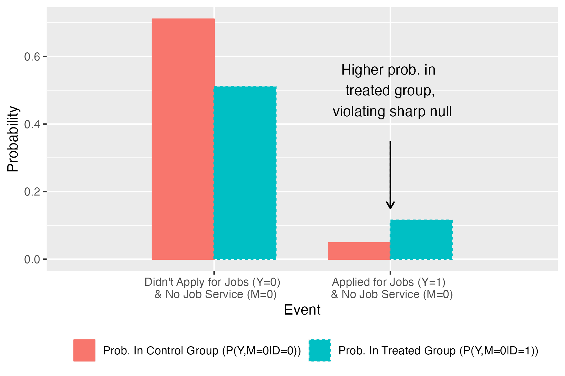
Figure 1: Illustration of Testable Implications in bursztyn_misperceived_2020

Note: This figure shows estimates of the probabilities $P(Y=y,M=0\mid D=d)$ for $d=0,1$ and $y=0,1$ in the application to bursztyn_misperceived_2020. For example, $P(Y=1,M=0\mid D=0)$ is the probability that one both applies for a job and does not sign up for the job-search service conditional on being in the control group. Under the sharp null of full mediation, it should be that $P(Y=y,M=0\mid D=0)\geq P(Y=y,M=0\mid D=1)$ for $y=0,1$. We see, however, that this inequality is violated in the empirical distribution for $y=1$: more women apply for jobs and don’t use the job-search service in the treated group, as indicated by the black arrow.

Since $Y$ is binary in our example, an implication of the inequalities in (2) from setting $A=\{1\}$ is

$$P(Y=1,M=0\mid D=0)\geq P(Y=1,M=0\mid D=1).$$

That is, there should be more women who apply for jobs and don’t sign up for the job-search service in the control group than the treated group. However, as shown in Figure 1, the empirical distribution shows that the opposite is true: there are more women who apply for jobs and don’t sign up for the job-search service in the treated group ($\hat{P}(Y=1,M=0\mid D=1)>\hat{P}(Y=1,M=0\mid D=0)$), indicating a violation of the sharp null. These differences are statistically significant at the 5% level, as we will describe in more detail in Section 5 below after we describe methods for conducting inference.

The data thus reject the sharp null hypothesis that the impact of the information treatment on job applications operates purely through job-search service sign-up. In particular, the data suggest that some never-takers must have their outcome affected by the treatment. We can thus conclude that there is some impact of changes in beliefs on job applications that does not operate mechanically through signing up for the job-search service.

The analysis so far highlights that tools originally developed for testing the LATE assumptions can be useful for testing hypotheses about mechanisms. However, several questions remain. First, our rejection of the null implies that the treatment affects the outcome through mechanisms other than job-search service sign-up, but how big are these alternative mechanisms? Second, our analysis relied on the monotonicity assumption that treatment increases job-search service sign-up, but what if we would like to relax this assumption? Third, while our motivating example had a binary $M$, in many examples we may be interested in testing that the treatment is explained by a non-binary mechanism, or by the combination of multiple mechanisms.

In the subsequent section, we develop a general theoretical framework that allows us to address all of these questions. Our framework accommodates mechanisms $M$ that are potentially multi-valued or multi-dimensional, and allows for relaxations of the monotonicity assumption. Further, in addition to deriving testable implications of the sharp null, we also derive lower bounds on the extent to which the alternative mechanisms matter—in particular, we derive bounds on the fraction of always-takers (or never-takers) that are affected by the treatment, as well as the average effect of the treatment for these always-takers.

3 Theory: General Case

We now consider the general case where $M$ is a $p$-dimensional vector with a finite number of possible support points $m_{0},...,m_{K-1}$. We denote by $G=lk$ the event that $M(0)=m_{l}$ and $M(1)=m_{k}$. We refer to individuals with $G=kk$ as the $k$-always takers, and individuals with $G=lk$ for $l\neq k$ as the $lk$-compliers. (Note that the terms “always-taker” and “complier” are used somewhat broadly here. For example, a “never-taker” in the case where $M$ is binary would be referred to as $0$-always taker, and likewise a defier would be a $10$-complier.) We denote by $\theta_{lk}:=P(M(0)=m_{l},M(1)=m_{k})$ the fraction of the population of type $G=lk$, and let $\theta$ be the vector in the $K^{2}$-dimensional simplex that collects the $\theta_{lk}$.

Extending the definition from the previous section, we say that the sharp null of full mediation holds if

$$Y(d,m)=Y(m)\text{ almost surely, for all }(d,m)^{\prime}\in\{0,1\}\times\{m_{0},...,m_{K-1}\}.$$

We note that if $M$ is multi-dimensional with, say, the first dimension corresponding to mechanism $A$ and the second corresponding to mechanism $B$, then the sharp null imposes that the treatment operates on $Y$ only through its joint effect on mechanisms $A$ and $B$.

We assume throughout that the treatment is independent of the potential outcomes and treatments. If the treatment were randomly assigned conditional on some observable $X$, then all of the restrictions we derive would be valid conditional on $X$ (see Section 6 for a discussion of extending these results to settings with instrumental variables).

Assumption 1 (Independence).

The treatment is independent of the potential outcomes and mediators, $D\perp\!\!\!\perp(Y(\cdot,\cdot),M(\cdot))$.

For our identification results, we allow for the researcher to place arbitrary restrictions on the shares of each compliance type.

Assumption 2 (Additional Restrictions).

$\theta\in R$ for $R\subseteq\Delta$, where $\Delta$ denotes the $K^{2}$-dimensional simplex.

We briefly review a few examples of restrictions that may be natural in some applications.

Example 1 (Monotonicity and relaxations thereof).

First, consider the case where $M$ is fully-ordered, so that $m_{0}<m_{1}<...<m_{K-1}$. This nests the binary example from the previous section as the special case where $K=2$. Then the monotonicity assumption that $M(1)\geq M(0)$ corresponds to the restriction

$$R=\{\theta\in\Delta:\theta_{lk}=0\text{ if }l>k\}.$$

One could also weaken this assumption by, for example, allowing for up to $\bar{d}$ fraction of the population to be defiers, which corresponds to setting

$$R=\left\{\theta\in\Delta:\sum_{l,k:l>k}\theta_{lk}\leq\bar{d}\right\}.$$

Example 2 (Partial monotonicity).

Suppose that $M$ is a $p$-dimensional vector for $p>1$. It may sometimes be reasonable to impose that each element of $M(d)$ is increasing in $d$. This can be achieved by setting

$$R=\left\{\theta\in\Delta:\theta_{lk}=0\text{ if }m_{l}\not\preceq m_{k}\right\},$$

where $m_{l}\preceq m_{k}$ if each element of $m_{l}$ is less-than-or-equal the corresponding element of $m_{k}$. Similar to the previous example, one could also allow for up to $\bar{d}$ fraction of the population to have $M(0)\not\preceq M(1)$.

Example 3 (Smoothness of $M(d)$).

In some settings, it may be reasonable to impose that the treatment does not have too large an effect on $M$, at least for most people. This could be formalized by setting

$$R=\left\{\theta\in\Delta:\sum_{\begin{subarray}{c}l,k\\ ||m_{l}-m_{k}||>\kappa\end{subarray}}\theta_{lk}\leq\bar{d}\right\}.$$

This imposes that at most $\bar{d}$ fraction of the population has $||M(1)-M(0)||>\kappa$.

Example 4 (No restrictions).

If the researcher is not willing to impose any restrictions on compliance types, then one can simply set $R=\Delta$.

It is worth nothing that all the restrictions given in the examples above can be written as linear restrictions on $\theta$, i.e. $R$ takes the polyhedral form $R=\{\theta:B\theta\leq c\}$ for a known matrix $B$ and vector $c$. Below, we will show that sets $R$ of this form facilitate straightforward computation via linear programming.

In what follows, we derive lower bounds on the extent to which the $k$-always takers are affected by the treatment despite having the same value of $M$ regardless of treatment status. In particular, in Section 3.1 we derive lower bounds on the fraction of $k$-always takers who are affected by the treatment. Since the sharp null of full mediation implies that this fraction is zero, we reject the sharp null if the lower bound on the fraction of $k$-always takers affected is non-zero for any $k$. In Section 3.2, we derive bounds on the average effect of the treatment for the $k$-always takers.

3.1 Bounds on fraction of always-takers affected

We now derive lower-bounds on the fraction of always-takers whose outcome is affected by the treatment despite having the same value of $M$ under both treatments. To be more precise, we define

$$\nu_{k}:=P(Y(1,m_{k})\neq Y(0,m_{k})\mid G=kk)$$

to be the fraction of $k$-always takers whose outcome is affected by the treatment despite always having $M=m_{k}$ under both treatments. The $\nu_{k}$ are a measure of the strength of mechanisms other than $M$: they tell us what fraction of the $k$-always takers have a direct effect of the treatment. Under the sharp null of full mediation, $Y(1,m_{k})=Y(0,m_{k})$ with probability 1, and thus $\nu_{k}=0$ for all $k$. By contrast, if $\nu_{k}$ is close to 1 for a particular $k$, then alternative mechanisms other than $M$ matter for nearly all $k$-always takers.

Our first main result provides a lower bound on $\nu_{k}$ as a function of the observable data and the type shares $\theta$. We will show that this bound is sharp in Section 3.1.1 below. To simplify notation, let

$$\Delta_{k}(A):=P(Y\in A,M=m_{k}\mid D=1)-P(Y\in A,M=m_{k}\mid D=0)$$

be the difference in the probability that $Y\in A,M=m_{k}$ between the treated and control groups. We then have the following lower bound on the fraction of $k$-always takers affected by the treatment.

Proposition 3.1.

Suppose Assumption 1 holds. Then for all $k=0,...,K-1$,

$$\theta_{kk}\nu_{k} \geq\sup_{A}\Delta_{k}(A)-\sum_{l:l\neq k}\theta_{lk}$$

$$=\sup_{A}\Delta_{k}(A)-\left(P(M=m_{k}\mid D=1)-\theta_{kk}\right).$$ (3)

where the $\sup$ is over all Borel sets $A$.

Recall that under the sharp null of full mediation, the fraction of always takers affected should be zero. We thus immediately obtain the following testable implications of the sharp null by setting $\nu_{k}=0$ in (3).

Corollary 3.1 (Testable implications of sharp null).

If Assumption 1 holds and the sharp null is satisfied, then for all $k=0,...,K-1$,

$$\sup_{A}\Delta_{k}(A)\leq\sum_{l:l\neq k}\theta_{lk}=P(M=m_{k}\mid D=1)-\theta_{kk}.$$ (4)

Proof sketch.

We now provide a short sketch of the proof of Proposition 3.1. Observe that individuals with $M=m_{k}$ when $D=1$ are either $k$-always takers or $lk$-compliers. Thus, we have that

$$P(Y\in A,M=m_{k}\mid D=1)=\theta_{kk}P(Y(1,m_{k})\in A\mid G=kk)+\sum_{l:l\neq k}\theta_{lk}P(Y(1,m_{k})\in A\mid G=lk).$$

Similarly, individuals with $M=m_{k}$ when $D=0$ are either $k$-always takers or $kl$-compliers, and so

$$P(Y\in A,M=m_{k}\mid D=0)=\theta_{kk}P(Y(0,m_{k})\in A\mid G=kk)+\sum_{l:l\neq k}\theta_{kl}P(Y(0,m_{k})\in A\mid G=kl).$$

From the previous two equations, it is then straightforward to solve for $P(Y(1,m_{k})\in A\mid G=kk)-P(Y(0,m_{k})\in A\mid G=kk)$. Using the fact that probabilities are bounded between 0 and 1 and taking a $\sup$ over all sets $A$, we then obtain the inequality

$$\theta_{kk}\left(\sup_{A}\left[P(Y(1,m_{k})\in A\mid G=kk)-P(Y(0,m_{k})\in A\mid G=kk)\right]\right)\geq\sup_{A}\Delta_{k}(A)-\sum_{l:l\neq k}\theta_{lk}.$$

Recall, however, that the total variation distance between distributions $P$ and $Q$ is defined as $\sup_{A}P(Y\in A)-Q(Y\in A)$. Letting $TV_{k}$ denote the total variation distance between $Y(1,m_{k})\mid G=kk$ and $Y(0,m_{k})\mid G=kk$, the previous display thus implies that

$$\theta_{kk}TV_{k}\geq\sup_{A}\Delta_{k}(A)-\sum_{l:l\neq k}\theta_{lk}.$$

However, as shown in borusyak_bounding_2015, the total variation distance between two potential outcomes distributions corresponds to a sharp lower bound on the fraction of individuals who are affected by the treatment, and thus we have that $TV_{k}\leq\nu_{k}$, which together with the inequality in the previous display yields the result in Proposition 3.1. $\Box$

Partially-identified shares.

If the type shares $\theta$ are point-identified, then Proposition 3.1 and Corollary 3.1 can be applied immediately to lower-bound the fraction of always-takers affected by the treatment and test the sharp null. This is the case, for example, in the setting in Section 2 with binary $M$ and a monotonicity assumption, where the share of always-takers and compliers is identified from the distribution of $M\mid D$. In more complicated settings, however, the type shares $\theta$ may only be partially identified, as illustrated in the following examples.

Example 5 (Binary $M$ without monotonicity).

Consider the case where $M$ is binary but we do not impose the monotonicity assumption. It is well-known in IV settings with a binary treatment and instrument that the share of defiers is not point-identified (e.g. huber_sharp_2017). Since we showed in Section 2 that our setting with binary $M$ is analogous to the IV setting, it follows that $\theta$ is not generically point-identified without a monotonicity assumption. As a concrete example, suppose that $P(M=1\mid D=1)=0.5$ and $P(M=1\mid D=0)=0.3$. Then the data is consistent with there being no defiers (by setting $\theta_{11}=0.3$, $\theta_{01}=0.2$, $\theta_{00}=0.5$, and $\theta_{10}=0$) but it is also consistent with up to 0.3 fraction of the population being defiers (by setting $\theta_{11}=0$, $\theta_{01}=0.5$, $\theta_{00}=0.2$, $\theta_{10}=0.3$).

Example 6 (Fully ordered, multi-valued $M$).

Partial identification of the shares also can arise if $M$ is fully-ordered but takes on multiple values (even under monotonicity). Consider the case where $M$ takes on 3 values ($0,1,2$) and the marginal distributions of $M\mid D$ are as given in Figure 2, panel (a). As can be seen in the figure, the treated group has a 0.2 higher probability that $M=2$ and a 0.2 lower probability that $M=0$ relative to the control group. This is consistent with 20% of the population being $02$-compliers and the remainder of the population being always-takers (i.e. $\theta_{02}=0.2$, $\theta_{01}=\theta_{12}=0$), as shown in Figure 2, panel (b). However, it is also consistent with a “cascade” in which 20% of the population is $01$-compliers, and another 20% of the population is $12$-compliers (i.e. $\theta_{01}=\theta_{12}=0.2$, $\theta_{02}=0$), as shown in Figure 2, panel (c).

(a)

(b)

(c)

Figure 2: Illustration of partial identification of type shares

We will denote by $\Theta_{I}$ the identified set for $\theta$, i.e. the set of possible joint distributions for $(M(0),M(1))$ that are consistent with the observed data and the restriction that $\theta\in R$. Concretely, we denote by $\Theta_{I}$ the set of $\theta$ such that

$$\sum_{l}\theta_{kl}=P(M=m_{k}\mid D=0)\text{ for }k=0,..,K-1\hskip 28.45274pt M\mid D=0$$ (Match marginals for )

$$\sum_{l}\theta_{lk}=P(M=m_{k}\mid D=1)\text{ for }k=0,..,K-1\hskip 28.45274pt M\mid D=1$$ (Match marginals for )

$$0\leq\theta_{kk^{\prime}}\leq 1\text{ for all $k,k^{\prime}$}\hskip 28.45274pt$$ (Probabilities in unit interval)

$$\theta\in R\hskip 28.45274pt \text{(Additional Restrictions)}.$$

It it worth noting that the first three restrictions above are linear in $\theta$. Thus, if $R$ is characterized by linear restrictions, then the identified set is a polyhedron, and quantities such as $\max_{\theta\in\Theta_{I}}\theta_{kk}$ can be calculated by linear programming.

Since Proposition 3.1 gives a lower bound on $\nu_{k}$ at the true shares $\theta$, which are contained within the identified set, it follows that $\nu_{k}$ is at least as large as the lowest lower bound implied by a $\theta$ in the identified set. It turns out that the lowest lower bound is achieved at the $\theta\in\Theta_{I}$ that minimizes the fraction of $k$-always takers, $\theta_{kk}$. This is intuitive since if $\theta_{kk}=0$, there are no $k$-always takers, and so it is impossible to obtain bounds on the fraction of $k$-always takers affected. When the number of $k$-always takers is small, it is thus difficult to learn about the fraction of $k$-always takers affected. The following corollary formalizes the implied lower bounds on $\nu_{k}$.

Corollary 3.2.

Suppose Assumptions 1 and 2 hold. Let $\theta_{kk}^{min}=\inf_{\theta\in\Theta_{I}}\theta_{kk}$. If $\theta_{kk}^{min}>0$, then

$$\nu_{k} \geq\inf_{\theta\in\Theta_{I}}\frac{1}{\theta_{kk}}\left(\sup_{A}\Delta_{k}(A)-\sum_{l:l\neq k}\theta_{lk}\right)$$

$$=\frac{1}{\theta_{kk}^{min}}\left(\sup_{A}\Delta_{k}(A)-\left(P(M=m_{k}\mid D=1)-\theta_{kk}^{min}\right)\right).$$

Similarly, Corollary 3.1 gives implications of the sharp null hypothesis involving the true shares $\theta$. Since the true $\theta$ is contained within the identified set, it follows that these restrictions must hold for some $\theta\in\Theta_{I}$.

Corollary 3.3.

Suppose Assumptions 1 and 2 hold. Then if the sharp null holds, there exists some $\theta\in\Theta_{I}$ such that $\sup_{A}\Delta_{k}(A)\leq P(M=m_{k}\mid D=1)-\theta_{kk}$ holds simultaneously for all $k=0,...,K-1$.

Note that when $\Theta_{I}$ is a polyhedron, then the implications of Corollary 3.3 can be tested simply via linear programming. In particular, the implications are satisfied if and only if the linear program

$$\min_{s\in\mathbb{R},\theta\in\Theta_{I}}s\text{ s.t. }\sup_{A}\Delta_{k}(A)\leq P(M=m_{k}\mid D=1)-\theta_{kk}+s\text{ for all $k$}$$ (5)

has a solution $s^{*}\leq 0$. It is thus straightforward to verify whether there exists a $\theta\in\Theta_{I}$ consistent with the sharp null and the observable data.

Remark 1 (Closed-form solution with fully-ordered, monotone $M$).

Consider the case where $M$ is fully-ordered and we impose monotonicity as in Example 1. In this case, it turns out that there is a closed-form solution for $\theta_{kk}^{min}$. Intuitively, to minimize the number of always-takers, we wish to have as many compliers as possible. This can be achieved by maximizing the amount of “cascading”, as in panel (c) of Figure 2. Proposition B.1 in the appendix formalizes this intuition, and shows that

$$\theta_{kk}^{min}=\max\{\underbrace{P(M=m_{k}\mid D=1)}_{\text{Point mass at $M=m_{k}$ when $D=1$}}-\hskip 14.22636pt\underbrace{P(M\geq m_{k}\mid D=1)-P(M\geq m_{k}\mid D=0)}_{\text{Treatment effect on survival fn of $M$ at $m_{k}$}}\hskip 2.84544pt,\hskip 2.84544pt0\}.$$ (6)

Moreover, there exists a $\theta\in\Theta_{I}$ such that $\theta_{kk}=\theta_{kk}^{min}$ simultaneously for all $k$. Thus, when $M$ is fully-ordered and we impose monotonicity, one need not use a linear program to lower bound $\nu_{k}$ or test the sharp null, but can simply plug in the value of $\theta_{kk}^{min}$ to the testable implications given in Corollaries 3.2 and 3.3.

Remark 2 (Identifying Power).

The testable implications we have derived for the sharp null are based on the fact that under the sharp null, there is no effect of the treatment on $k$-always takers (i.e. $\nu_{k}=0$). Intuitively, it is harder to obtain non-trivial lower bounds on $\nu_{k}$ the fewer $k$-always takers there are. Indeed, if there were no always-takers for any $k$, then our testable implications would be satisfied trivially. This can be seen more formally by observing that the inequalities in Corollary 3.3 are harder to satisfy the larger is $\theta_{kk}$. The expression for $\theta_{kk}^{min}$ in (6) is thus informative about when the testable implications will have bite. In particular, it shows that $\theta_{kk}^{min}$ will tend to be large when there is substantial point mass at $M=m_{k}$ in the treated group, and when the treatment effect on the survival function is small at $M=m_{k}$. Thus, while our testable implications are valid regardless of how many support points for $M$ there are, there will tend to be more identifying power when there is substantial point mass for at least some values of $M$.

Remark 3 (Binning values of $M$).

In light of the previous remark, in settings where the original $M$ is continuous or discrete with many values, it may be tempting to discretize the original $M$ into a small number of bins, and then apply the tests above with the discretized value of $M$ to increase power. Under such a discretization, our tests for the sharp null remain valid if one imposes that $Y(d,m)=Y(d,m^{\prime})$ for all $m,m^{\prime}$ in the same bin, i.e. changes of $M$ within a bin do not affect the outcome. This is, of course, a strong assumption if taken literally. However, one might reasonably expect that a small change in $M$ should not affect the outcome for most people. This could be captured by the assumption that $P(Y(d,m)\neq Y(d,m^{\prime})\mid G=kk)\leq\nu_{max}$ for all $m,m^{\prime}$ in the same bin, i.e. changes of $M$ within a bin affect at most $\nu_{max}$ fraction of always-takers. Under this assumption, at most $\nu_{max}$ fraction of always-takers should be affected using the discretized $M$, and thus we can reject the sharp null if the lower bound on $\nu_{k}$ given in Corollary 3.3 using the discretized $M$ exceeds $\nu_{max}$.

Remark 4 (Functions of the $\nu_{k}$).

We may sometimes be interested in aggregations of the $\nu_{k}$ across $k$. For example, the total fraction of always-takers whose outcome is affected by treatment, pooling across $k$, is given by

$$\bar{\nu}:=P(Y(1,M(1))\neq Y(0,M(0))\mid M(1)=M(0))=\frac{\sum_{k}\theta_{kk}\nu_{k}}{\sum_{k}\theta_{kk}}.$$

To compute a lower bound on this quantity, we must find $\theta$ and $\nu$ to minimize $\frac{\sum_{k}\theta_{kk}\nu_{k}}{\sum_{k}\theta_{kk}}$ subject to the constraints that (3) holds and $\theta\in\Theta_{I}$. If we reparameterize the problem in terms of $\theta$ and $\tilde{\nu}_{k}:=\theta_{kk}\nu_{k}$, then both the numerator and denominator of the objective are linear in the parameters, and the constraints are also linear in the parameters if $R$ is a polyhedron. Thus, the problem of minimizing $\frac{\sum_{k}\theta_{kk}\nu_{k}}{\sum_{k}\theta_{kk}}$ over the identified set is a linear-fractional program, which can be recast as a simple linear program via the charnes_programming_1962 transformation. It is thus simple to solve for lower bounds on the total fraction of always-takers affected by treatment, pooling across $k$.

Remark 5 (Connections to IV testing).

Since testing the sharp null of full mediation is analogous to testing instrument validity—with $M$ playing the role of the endogenous variable and $D$ the instrument—Corollary 3.3 immediately implies testable implications for instrument validity in settings with a binary instrument and multi-valued $M$. Further, we show in the next section that these testable implications are in fact sharp. The sharp testable restrictions derived here thus may be of independent interest for the problem of testing instrument validity. sun_instrument_2023 derived non-sharp testable implications of instrument validity in the setting where $M$ is multi-valued but fully-ordered and one imposes monotonicity. His testable restrictions involve only the observable distributions with the minimum and maximal value of $M$. By contrast, Corollary 3.3 shows that there are in fact testable restrictions coming from all possible values of $M$, and adding these additional restrictions makes the testable impliations sharp. Moreover, while sun_instrument_2023’s results apply under a monotonicity assumption, our results also imply testable implications under relaxations of monotonicity via a suitable choice of $R$, as described in Examples 1-4 above.

3.1.1 Sharpness of Bounds

So far we have provided lower bounds on the fraction of $k$-always takers who were affected by treatment, $\nu_{k}$. These lower bounds in turn implied testable implications for the sharp null, under which $\nu_{k}=0$ for all $k$. We now show that the testable implications from the previous section are sharp, in the sense that they exhaust all the testable content in the data. In particular, we will show there exists a data-generating process for the potential outcomes and mediators consistent with the observable data such that the lower bounds for the $\nu_{k}$ in Proposition 3.1 hold with equality. As a corollary, if the testable implications of the sharp null are satisfied, then there exists a DGP for the potential outcomes and mediators consistent with the observable data such that the sharp null is satisfied.

We first formalize what we mean for a distribution of potential outcomes to be consistent with the observable data. Recall that $P$ denotes the distribution of the observable data $(Y,M,D)$. Let $P^{*}$ be a distribution over the model primitives $(Y(\cdot,\cdot),M(\cdot,\cdot),D)$. We say that the distribution $P^{*}$ is consistent with the observable data if the distribution of $(Y(D,M(D)),M(D),D)$ under $P^{*}$ is equal to $P$—that is, $P^{*}$ is a distribution of the model primitives that leads to observable data $P$.

Our first result then shows that the lower bounds on $\nu_{k}$ derived in Proposition 3.1 are sharp: i.e. there exists a $P^{*}$ consistent with the observable data under which the inequalities hold with equality.

Proposition 3.2.

For any $\theta\in\Theta_{I}$, there exists a distribution $P^{*}$ for $(Y(\cdot,\cdot),M(\cdot),D)$ consistent with the observable data and satisfying Assumptions 1 and 2 such that for all $k=0,...,K-1$,

$$\left(\sup_{A}\Delta_{k}-\sum_{l:l\neq k}\theta_{lk}\right)_{+}=\theta_{kk}\nu_{k},$$ (7)

where $\nu_{k}=P^{*}(Y(1,m_{k})\neq Y(0,m_{k})\mid G=kk)$, $\theta_{lk}=P^{*}(M(0)=m_{l},M(1)=m_{k})$, and $(x)_{+}:=\max\{x,0\}$.

It follows immediately from Proposition 3.2 that the implications of the sharp null derived in Corollary 3.1 are sharp.

Corollary 3.4.

Suppose that there is some $\theta\in\Theta_{I}$ such that (4) holds for all $k=0,...,K-1$. Then there exists a distribution $P^{*}$ for $(Y(\cdot,\cdot),M(\cdot),D)$ consistent with the observable data and satisfying Assumptions 1 and 2 such that the sharp null holds.

3.2 Bounds on average effects for always-takers

So far we have provided lower bounds on $\nu_{k}$, the fraction of $k$-always takers who are affected by the treatment despite having $M=m_{k}$ under both treatments. The $\nu_{k}$ provide a measure of what fraction of always-takers are affected by alternative mechanisms. However, in some settings we may also be interested in the magnitude of the alternative mechanisms for the always-takers. In this section, we derive bounds on

$$ADE_{k}:=E[Y(1,m_{k})-Y(0,m_{k})\mid G=kk],$$

the average direct effect of the treatment on the outcome for the $k$-always takers. This provides an alternative measure of the size of the alternative mechanisms for the always-takers.

To derive bounds for $ADE_{k}$, we first derive bounds on $E[Y(1,m_{k})\mid G=kk]$. Observe that individuals with $M=m_{k},D=1$ must be either $k$-always takers or $lk$-compliers. The share of $k$-always takers among this population is given by $\tilde{\theta}_{kk}^{1}:=P(G=kk\mid D=1,M=m_{k})=\frac{\theta_{kk}}{P(M=m_{k}\mid D=1)}$. It follows that the observable distribution of $Y\mid D=1,M=m_{k}$ is a mixture with weight on $\tilde{\theta}_{kk}^{1}$ on $Y(1,m_{k})\mid G=kk$ and weight $(1-\tilde{\theta}_{kk}^{1})$ on the distribution of $Y(1,m_{k})$ for $lk$-compliers. We can thus obtain bounds on $E[Y(1,m_{k})\mid G=kk]$ by considering the worst-case scenario where the $k$-always takers compose the bottom $\tilde{\theta}_{kk}$ fraction of the $Y\mid D=1,M=m_{k}$ distribution, and the best-case scenario where they compose the top $\tilde{\theta}_{kk}$.

The following lemma formalizes this intuition for obtaining bounds on $E[Y(1,m_{k})\mid G=kk]$, and applies analogous logic to obtain bounds on $E[Y(0,m_{k})\mid G=kk]$. For ease of notation, we present results in the main text assuming that the distribution of $Y$ is continuous; analogous results without this assumption are given in Lemma A.3 in the Appendix.

Lemma 3.1.

Suppose Assumption 1 holds and that $Y$ is continuously distributed. Let $y^{d}_{q}:=F^{-1}_{Y\mid D=d,M=m_{k}}(q)$ be the $q$th quantile of $Y\mid D=d,M=m_{k}$. If $\tilde{\theta}_{kk}^{1}>0$, then

$$E[Y\mid M=m_{k},D=1,Y\leq y^{1}_{\tilde{\theta}_{kk}^{1}}]\leq E[Y(1,m_{k})\mid G=kk]\leq E[Y\mid M=m_{k},D=1,Y\geq y^{1}_{1-\tilde{\theta}_{kk}^{1}}].$$

Likewise, if $\tilde{\theta}_{kk}^{0}>0$, then

$$E[Y\mid M=m_{k},D=0,Y\leq y^{0}_{\tilde{\theta}_{kk}^{0}}]\leq E[Y(0,m_{k})\mid G=kk]\leq E[Y\mid M=m_{k},D=0,Y\geq y^{0}_{1-\tilde{\theta}_{kk}^{0}}].$$

The bounds are sharp in the sense that there exists a distribution $P^{*}$ for $(Y(\cdot,\cdot),M(\cdot),D)$ consistent with the observable data and with $\theta_{lk}=P^{*}(G=lk)$ such that the bounds hold with equality.

Lemma 3.1 immediately implies bounds on $ADE_{k}$ by differencing the inequalities for the expectations of $Y(1,m_{k})$ and $Y(0,m_{k})$. Note, however, that the bounds in Lemma 3.1 involve the always-taker share $\tilde{\theta}_{kk}^{d}=\frac{\theta_{kk}}{P(M=m_{k}\mid D=d)}$, which may only be partially identified. It is straightforward to see, however, that the bounds become wider the smaller is $\tilde{\theta}_{kk}^{d}$. Intuitively, this is because the most-favorable subdistribution of fraction $\tilde{\theta}_{kk}^{d}$ is more favorable the smaller is $\tilde{\theta}_{kk}^{d}$, and likewise for the least-favorable subdistribution. Sharp bounds on $ADE_{k}$ can thus be obtained by plugging $\theta_{kk}^{min}$ into the bounds given in Lemma 3.1. For notation, let $LB_{1}(\tilde{\theta}^{1}_{kk})$ and $UB_{1}(\tilde{\theta}^{1}_{kk})$ denote the lower- and upper-bounds on $E[Y(1)\mid G=kk]$ given in Lemma 3.1 as a function of $\tilde{\theta}^{1}_{kk}$. We define $LB_{0}(\tilde{\theta}^{0}_{kk})$ and $UB_{0}(\tilde{\theta}^{0}_{kk})$ analogously, replacing $Y(1)$ with $Y(0)$. We then have the following bounds on $ADE_{k}$.

Proposition 3.3.

Suppose Assumption 1 holds and $Y$ is continuously distributed. If $\theta_{kk}^{min}=\inf_{\theta\in\Theta_{I}}\theta_{kk}>0$, then sharp bounds on $ADE_{k}$ are given as follows:

$$LB_{1}(\tilde{\theta}_{kk}^{1,min})-UB_{0}(\tilde{\theta}_{kk}^{0,min})\leq ADE_{k}\leq UB_{1}(\tilde{\theta}_{kk}^{1,min})-UB_{0}(\tilde{\theta}_{kk}^{0,min})$$

where $\tilde{\theta}_{kk}^{d,min}=\frac{\theta_{kk}^{min}}{P(M=m_{k}\mid D=d)}$. The lower and upper bounds are each sharp in the sense that there exists a distribution $P^{*}$ for $(Y(\cdot,\cdot),M(\cdot),D)$ consistent with the observable data and Assumption 1 and Assumption 2 such that the bound holds with equality.

It is worth noting that in the simple case where $M$ is binary and one imposes monotonicity, the bounds on $ADE_{k}$ correspond to lee_training_2009’s bounds, where $D$ is viewed as the treatment and $M$ as the “sample selection”. In the binary case, the $ADE_{k}$ can also be viewed as what the statistics literature refers to as principal strata direct effects for the principal strata with $M(1)=M(0)=m_{k}$ (frangakis_principal_2002; zhang_estimation_2003). flores_nonparametric_2010 observed that such bounds could be used for mediation analysis in the case of binary $M$—their Proposition 1 matches the bounds given in Lemma 3.1 for the special case where $M$ is binary—although they use this primarily as an intermediate steps to derive bounds on the population direct effect of treatment. Our result extends these existing results for the binary case to settings where $M$ may be multi-valued (and where monotonicity may fail).

It is also worth emphasizing that the sharp null of full mediation considered earlier is distinct from the null hypothesis that $ADE_{k}=0$ for all $k$. In particular, the sharp null imposes that the treatment does not have an effect on the outcome for any always-taker, whereas the null that $ADE_{k}=0$ imposes that the treatment does not affect the $k$-always takers on average. This is analogous to the distinction between the sharp null considered by Fisher and the weak null considered by Neyman, applied to the sub-population of always-takers. Thus, we may be able to reject the sharp null in settings where we cannot reject the weaker null that the $ADE_{k}$ are zero.

4 Inference

The previous section derived testable implications of the sharp null of full mediation, as well as measures of the extent to which it is violated, which involved the distribution of the observable data $(Y,M,D)\sim P$. We now derive methods for inference on the sharp null given a sample of $N$ $iid$ observations (or clusters) drawn from $P$, $(Y_{i},M_{i},D_{i})_{i=1}^{N}$. For simplicity of notation, we focus on testing the sharp null, although a simple adaptation of the described approach can be used to test null hypotheses of the form $H_{0}:\nu_{k}\leq\nu^{ub}_{k}$ for any $\nu^{ub}_{k}$ (with the sharp null the special case with $\nu^{ub}_{k}=0$ for all $k$.)

We first comment on the non-standard nature of the inference problem. Recall that the testable implications of the sharp null are equivalent to whether the linear program (5) has a weakly negative solution. However, functions of the observable data enter the constraints of the linear program, and it is well-known that the solution to a linear program can be non-differentiable in the constraints. Second, the function of the observable data in the constraints, $\sup_{A}\Delta_{k}(A)$, is itself potentially non-differentiable in the underlying data-generating process. If the outcome $Y$ is continuously distributed, for example, then $\sup_{A}\Delta_{k}(A)=\int(f_{Y,M=m_{k}\mid D=1}(y)-f_{Y,M=m_{k}\mid D=0}(y))_{+}\,dy$, where $(x)_{+}=\max\{x,0\}$, which is clearly non-differentiable in the underlying partial densities if $f_{Y,M=m_{k}\mid D=1}(y)=f_{Y,M=m_{k}\mid D=0}(y)$ on a set of positive measure. Since bootstrap methods are generally invalid when the target parameter is non-differentiable in the underlying data-generating process (fang_inference_2019), we cannot simply bootstrap the solution to (5).

We now show that methods from the moment inequality literature can be used to circumvent these issues. We focus on the case where the distribution of $Y$ is discrete, with support points $y_{1},...,y_{Q}$. As we discuss in Remark 6 below, if $Y$ is continuous, then the tests we derive remain valid if one uses a discretization of $Y$, although at the potential loss of sharpness. We also focus on the case where $R$ takes the polyhedral form $R=\{\theta\in\Delta:B\theta\leq c\}$. To see the connection with moment inequalities, observe that with discrete $Y$, we have that

$$\sup_{A}\Delta_{k}(A)=\sum_{q=1}^{Q}\left(P(Y=y_{q},M=m_{k}\mid D=1)-P(Y=y_{q},M=m_{k}\mid D=0)\right)_{+}$$

where again $(x)_{+}=\max\left\{x,0\right\}$. It follows that the inequality

$$\sup_{A}\Delta_{k}(A)\leq P(M=m_{k}\mid D=1)-\theta_{kk}$$

holds if and only if there exist $\delta_{k1},...,\delta_{kq}$ such that

$$\sum_{q=1}^{Q}\delta_{kq}\leq P(M=m_{k}\mid D=1)-\theta_{kk}$$ (8)

$$\delta_{kq}\geq P(Y=y_{q},M=m_{k}\mid D=1)-P(Y=y_{q},M=m_{k}\mid D=0)\text{ for }q=1,...,Q$$ (9)

$$\delta_{kq}\geq 0\text{ for }q=1,...,Q$$ (10)

Hence, the testable implications of the sharp null derived in Corollary 3.3 are equivalent to the statement that there exists some $\theta\in\Theta_{I}$ and $\delta$ such that (8)-(10) hold for all $k=0,...,K-1$.

Observe, further, that $\delta,\theta$ and the observable probabilities enter the inequalities (8)-(10) linearly, and the same is true for the constraints that determine the identified set. Letting $\omega=(\theta^{\prime},\delta^{\prime})^{\prime}$, it follows that we can write the testable implications of the model in the form

$$C_{1}\,\omega-C_{2}\,p\geq 0,$$

where $C_{1},C_{2}$ are known matrices (not depending on the data) and $p$ is a vector that collects probabilities of the form $P(Y=y_{q},M=m_{k}\mid D=d)$ and $P(M=m_{k}\mid D=d)$. Let $\hat{p}$ denote the sample analog to $p$. Since $E[\hat{p}]=p$, we can write the testable implications of the sharp null as

$$H_{0}:\exists\,\omega\text{ s.t. }E[C_{1}\omega-C_{2}\hat{p}]\geq 0.$$ (11)

Moment inequalities of this form—in which the nuisance parameter $\omega$ enters the moments linearly and with known coefficients $C_{1}$—have been studied recently by andrews_inference_2023, cox_simple_2022, fang_inference_2023, and cho_simple_2023. The existing methods from the aforementioned papers can thus be used directly to test the sharp null of full mediation.

Remark 6 (Discretizing continuous outcomes).

Suppose that the outcome $Y$ is continuously distributed. Let $I_{1},...,I_{Q}$ be disjoint intervals that partition the outcome space, and let $Y^{disc}$ be the discretization of $Y$ that equals $j$ when $Y\in I_{j}$. Let $\Delta_{k}^{disc}(A)$ be the analog to $\Delta_{k}(A)$ using $Y^{disc}$ instead of $Y$. Observe that

$$\sup_{A}\Delta_{k}^{disc}(A) =\sup_{A}P(Y^{disc}\in A,M=m_{k}\mid D=1)-P(Y^{disc}\in A,M=m_{k}\mid D=0)$$

$$=\sup_{A\in\mathcal{A}_{disc}}P(Y\in A,M=m_{k}\mid D=1)-P(Y\in A,M=m_{k}\mid D=0)=\sup_{A\in\mathcal{A}_{disc}}\Delta_{k}(A)$$

where $\mathcal{A}_{disc}$ is the $\sigma$-algebra generated by $I_{1},...,I_{Q}$. Since $\mathcal{A}_{disc}$ is a subset of the Borel $\sigma$-algebra, it follows that $\sup_{A}\Delta_{k}^{disc}(A)\leq\sup_{A}\Delta_{k}(A)$. Hence, the testable implications of the sharp null for $Y$ imply the testable implications of the sharp null for any discretization of $Y$. One can thus obtain valid inference on the sharp null by discretizing the outcome and then using the approach described above with $Y^{disc}$. Of course, to retain approximate sharpness of the testable implications, one would like to choose a discretization fine enough such that $\sup_{A}\Delta^{disc}_{k}(A)\approx\sup_{A}\Delta_{k}(A)$. Observe that with a continuous outcome, $\sup_{A}\Delta^{disc}_{k}(A)=\sup_{A}\Delta_{k}(A)$ if the sign of $f_{Y,M=m_{k}\mid D=1}(y)-f_{Y,M=m_{k}\mid D=0}(y)$ is constant at all $y$ within the same interval $I_{j}$. To obtain approximate sharpness of the testable implications, one would thus like to choose a discretization such that there is a cut-point close to any point where the partial densities cross. A practical tradeoff arises, however, because making the discretization finer increases the number of moment inequalities needed to test, and the validity of the methods described above relies on the number of moments being sufficiently small relative to the sample size for a central limit theorem to approximate the distribution of $\hat{p}$. Moreover, the power of moment inequality methods may depend on the number of moments included. Although a formal treatment of the optimal discretization is beyond the scope of this paper, we explore the impact of discretization in our Monte Carlo simulations below.

4.1 Monte Carlo

To evaluate the methods for inference described above, we conduct Monte Carlo simulations calibrated to our applications to bursztyn_misperceived_2020 and baranov_maternal_2020 in Section 5 below. We focus on testing the sharp null under a monotonicity assumption.

Outcomes and mediators.

The outcome, mediator(s), and treatment in our simulations match those in our empirical applications. For bursztyn_misperceived_2020, the outcome is a binary indicator for applying for jobs outside of the home, and the mediator is a binary indicator for job-search service sign-up. For baranov_maternal_2020, the outcome is an index of financial empowerment. We consider two mediators, a binary indicator for the presence of a grandmother in the household, and a relationship-quality score, which is a score on a 1-5 scale.

Sample sizes.

The sample used for our main analysis of bursztyn_misperceived_2020 contains $284$ people, with treatment assignment randomized at the individual level (approximately half ($139$ ) were treated). For the simulations calibrated to bursztyn_misperceived_2020, we draw $284$ $iid$ observations to match the original sample size. In baranov_maternal_2020, treatment was assigned at the level of a cluster (i.e. at the Union Council level), with a total of 40 clusters (20 treated, 20 control), and a total sample size of approximately 600 individuals ($568$ or $585$ depending on the choice of $M$). For simulations calibrated to baranov_maternal_2020, we therefore draw 20 independent clusters from each treatment group. Given the small number of clusters, we expect this to be a relatively challenging setting for inference. To evaluate the impact of having a small number of clusters, we also consider alternative simulation designs where we sample 40 or 100 clusters of each treatment type, with a total of 80 and 200 clusters for each design.

Description of DGP.

In all of our simulations, we sample the distribution of $(Y,M)$ for control units from the empirical distribution of control units in our applications (i.e. from $(Y,M)\mid D=1$). For treated units in our simulations, we draw with probability $t$ from the empirical distribution of $(Y,M)$ for treated units, and with probability $1-t$ from the empirical distribution for control units, where $t\in\{0,0.5,1\}$ is a simulation parameter. Thus, when $t=1$, we are sampling both treated and control units in the simulation from the empirical distribution in the data, under which the sharp null is violated. This allows us to assess the power of the various tests. When $t=0$, on the other hand, the distribution of $(Y,M)$ for both treated and control units in the simulation is drawn from the empirical distribution for control units in the original data. This ensures that the testable implications of the sharp null are satisfied, which allows us to evaluate size control. (In fact, the design ensures that all of the implied moment inequalities hold with equality, which is generally a challenging setting for size control for moment inequality methods.) When $t=0.5$, the distribution of $(Y,M)$ for treated units is a mixture of the empirical distribution for treated and control units in the original data. Thus, the sharp null is violated, but the violation is smaller than under the case when $t=1$. Comparing across the cases $t=0.5$ and $t=1$ thereby allows us to evaluate how the power tests changes with the size of the violation of the null.

Table 1: Simulation results for binary $M$

Panel A: Bursztyn et al
	$\bar{\nu}$ LB	ARP	CS	K	FSSTdd	FSSTndd
t=0	$0$	$0.038$	$0.032$	$0.030$	$0.078$	$0.070$
t=0.5	$0.036$	$0.196$	$0.190$	$0.116$	$0.214$	$0.194$
t=1	$0.077$	$0.626$	$0.632$	$0.386$	$0.620$	$0.584$
Panel B: Baranov et al, 40 clusters
	$\bar{\nu}$ LB	ARP	CS	K	FSSTdd	FSSTndd
t=0	$0$	$0.056$	$0.154$	$0.050$	$0.232$	$0.212$
t=0.5	$0.134$	$0.194$	$0.206$	$0.064$	$0.314$	$0.270$
t=1	$0.283$	$0.570$	$0.668$	$0.422$	$0.750$	$0.680$
Panel C: Baranov et al, 80 clusters
	$\bar{\nu}$ LB	ARP	CS	K	FSSTdd	FSSTndd
t=0	$0$	$0.044$	$0.064$	$0.040$	$0.132$	$0.112$
t=0.5	$0.134$	$0.322$	$0.340$	$0.160$	$0.410$	$0.322$
t=1	$0.283$	$0.836$	$0.936$	$0.846$	$0.956$	$0.936$
Panel D: Baranov et al, 200 clusters
	$\bar{\nu}$ LB	ARP	CS	K	FSSTdd	FSSTndd
t=0	$0$	$0.044$	$0.054$	$0.030$	$0.120$	$0.090$
t=0.5	$0.134$	$0.686$	$0.776$	$0.618$	$0.776$	$0.734$
t=1	$0.283$	$0.998$	$1$	$1$	$1$	$1$

• Notes: This table contains simulation results for the DGPs where we have a binary mediator. The first column shows the value of $t$, which determines the distance from the null, as described in the main text. The second column shows the lower-bound on the fraction of always-takers affected by treatment, $\bar{\nu}$. The remaining columns contain the rejection probabilities for each of the methods considered. Panel A shows the results for the DGP based on bursztyn_misperceived_2020 and Panels B-D show the results for the DGPs based on baranov_maternal_2020, with the binary grandmother mediator, under different numbers of clusters. In Panels B-D, we use a discretization of the outcome into 5 bins for all tests except the K test. Rejection probabilities are computed over 500 simulation draws, under a 5% nominal significance level.

Methods used.

To implement tests based on moment inequalities as described above, we consider the hybrid test proposed by andrews_inference_2023, the conditional conditional chi-squared test proposed by cox_simple_2022, and the test proposed by fang_inference_2023. For comparison to existing methods in the case where $M$ is binary, we consider the test for instrument validity proposed by kitagawa_test_2015. In the simulations calibrated to bursztyn_misperceived_2020, the outcome is binary, and thus no discretization of the outcome is needed. For the simulations calibrated to baranov_maternal_2020, where the outcome takes many values, for the moment inequality methods we consider a discretization of the outcome based on 5 bins in our main specification (see Remark 6). We also consider alternative specifications using 2 and 10 bins. Since the K test does not require a discrete outcome, we use the original continuous outcome when implementing the K test. Implementation of the FSST test requires specifying the moment-selection tuning parameter $\lambda$. We consider the two choices recommended by FSST in their Remark 4.2, one of which is data-driven and the other is not. We refer to the resulting tests as FSSTdd and FSSTndd (where ‘dd’ denotes data-driven). For CS and ARP, we use analytic estimates of the variance of the moments, assuming the data are drawn $iid$ in the simulations calibrated to bursztyn_misperceived_2020, or that clusters are drawn $iid$ in the simulations calibrated to baranov_maternal_2020. Since the K and FSST tests require bootstrap replicates, we use a non-parametric bootstrap at either the individual or cluster level, as appropriate. All tests are implemented with nominal size of 5%.

Simulation Results.

Table 1 reports the results for simulations designs where we have a binary mediator. This includes the DGP based on bursztyn_misperceived_2020 (Panel A), and the DGPs that are based on baranov_maternal_2020 where the considered mediator is the binary indicator for the presence of a grandmother (Panels B-D). Table 2 shows results calibrated to baranov_maternal_2020 using the non-binary relationship quality variable as the mediator. Both tables show the rejection probabilities for each of the methods described above under different simulation designs. To quantify the magnitude of the violations of the sharp null, the table also reports the lower-bound on the fraction of always-takers affected ($\bar{\nu}$).

We first evaluate size control. Recall that DGPs with $t=0$ impose the sharp null of full mediation. Across nearly all simulation designs, we find that the ARP, CS, and K tests have close to nominal size, with rejection probabilities no larger than 9% for a 5% test. The one notable exception is the simulations in Panel B of Table 1, where there are only 40 independent clusters, in which case CS is somewhat over-sized, with a null rejection probability of 0.15. Doubling the number of clusters to 80 (Panel C) restores approximate size control, however. The FSST tests often have reasonable size control for settings with a large number of independent observations or clusters, but can be substantially over-sized in settings with a small or moderate number of clusters using the two default choices of tuning parameters, particularly with multi-valued $M$ (e.g. rejection probabilities of 0.274 and 0.178 in Table 2, Panel A).

We next evaluate power, focusing on the simulations with $t=0.5$ and $t=1$ under which the null is violated. Across all of the simulation designs, the CS test has power similar to or greater than that of ARP. The differences can be substantial in some cases, particularly with multi-valued $M$ (e.g. power of $0.96$ vs $0.16$ in Panel B of Table 2). Likewise, the power of the FSST tests is similar to or exceeds that of the CS test across nearly all simulation designs, although this comparison must be taken with some caution in cases where the FSST test appears to be over-sized. Finally, we note that in all of the simulations with binary $M$ (LABEL:tab:_app_sim_baranov_binM), the power of the three moment inequality tests (ARP, CS, FSST) is either similar to or exceeds that of the K test. This is the case both when the outcome is binary (Panel A), and when the outcome is approximately continuous (Panels B-D). Recall that when the outcome is continuous, the moment inequality tests use a discretization of the outcome to 5 bins, whereas the K test does not use a discretization. The favorable power comparisons in Panels B-D thus suggest that discretization does not come at a large loss of power in this simulation design, although of course this conclusion may be specific to the particular DGP studied here.

Table 2: Simulation results for non-binary $M$

Panel A: Baranov et al, 40 clusters
	$\bar{\nu}$ LB	ARP	CS	FSSTdd	FSSTndd
t=0	$0$	$0.052$	$0.088$	$0.274$	$0.178$
t=0.5	$0.119$	$0.066$	$0.228$	$0.438$	$0.374$
t=1	$0.255$	$0.166$	$0.754$	$0.864$	$0.828$
Panel B: Baranov et al, 80 clusters
	$\bar{\nu}$ LB	ARP	CS	FSSTdd	FSSTndd
t=0	$0$	$0.066$	$0.048$	$0.188$	$0.128$
t=0.5	$0.119$	$0.066$	$0.314$	$0.582$	$0.500$
t=1	$0.255$	$0.164$	$0.962$	$0.994$	$0.990$
Panel C: Baranov et al, 200 clusters
	$\bar{\nu}$ LB	ARP	CS	FSSTdd	FSSTndd
t=0	$0$	$0.046$	$0.026$	$0.144$	$0.108$
t=0.5	$0.119$	$0.076$	$0.542$	$0.862$	$0.824$
t=1	$0.255$	$0.286$	$1$	$1$	$1$

• Notes: This table contains simulation results for the DGPs where we have a non-binary mediator. The first column shows the value of $t$, which determines the distance from the null, as described in the main text. The second column shows the lower-bound on the fraction of always-takers affected by treatment, $\bar{\nu}$. The remaining columns contain the rejection probabilities for each of the inference methods considered. Each panel contains results for the DGPs based on baranov_maternal_2020, where the non-binary relationship-quality mediator is considered, for different numbers of clusters. Rejection probabilities are computed over 500 simulation draws, under a 5% nominal significance level.

In LABEL:tab:_app_sim_baranov_binM and LABEL:tab:_app_sim_baranov_nonbinM we present results for simulations calibrated to baranov_maternal_2020 using a discretization with 2 or 10 bins, rather than the 5 considered here. The patterns are qualitatively similar to those reported above. We again find good size control for CS and ARP in nearly all specifications. The one exception is again size control for CS in the setting calibrated to baranov_maternal_2020 with binary $M$ and 40 clusters. Relative to our baseline simulation with 5 bins, we find that size control improves when using 2 bins, and becomes worse when using 10 bins. This is intuitive, since the number of moments used increases with the bin size, and thus we expect the quality of the central limit theorem approximation to be worse with more bins. In terms of power, we do not find an obvious pattern across bin sizes, with power increasing in the number of bins for some tests/DGPs and decreasing for others. This reflects the fact that although the testable implications become sharper the more bins are used (see Remark 6), the finite-sample properties of the tests depend on the number of moments, and thus power may decrease when increasing the number of moments. Considering the balance of size control and power, 5 bins seems a reasonable default choice based on our simulations, although more formal guidance on the optimal number of bins strikes us as an interesting avenue for future research.

Recommendation.

Based on our simulations, CS strikes us a reasonable default choice for most empirical settings, given that it has approximate size control across most of our simulation designs and favorable power relative to ARP. However, ARP performs somewhat better in terms of size control in settings with a small number of clusters, and thus may be an attractive alternative for researchers concerned about size control in such settings, albeit at the loss of some power (particularly with multi-valued $M$). Likewise, FSST may offer power improvements relative to CS in settings with a large number of independent observations, so that size control is not a concern. In our applications below, we report results for CS in the main text; analogous results for ARP and FSST are given in LABEL:tbl:pvals.

5 Empirical applications

5.1 bursztyn_misperceived_2020 revisited

We now revisit our application to bursztyn_misperceived_2020 from Section 2. Recall that our treatment $D$ is random assignment to an information treatment about other men’s beliefs about women working outside the home, $M$ is sign-up for the job-search service, and $Y$ is an indicator for whether the wife applies for jobs outside of the home. For our main specification, we restrict attention to the majority of men who at baseline under-estimate other men’s beliefs, so that the monotonicity assumption that treatment weakly increases job-search service is plausible. (We find similar results when including all men; see Appendix D.)

Statistical significance.

Recall from Figure 1 that the testable implications of the sharp null were rejected based on the empirical distribution. Using the approach to inference described above, we find these violations are in fact statistically significant, with a $p$-value of $0.02$ using the CS test. The data thus provides strong evidence that the impact of the information treatment on long-run labor market outcomes does not operate solely through the sign-up for the job-search service. In particular, there are some never-takers who would not sign up for the service under either treatment who are nevertheless induced to apply for jobs by the treatment. We thus see that, for at least some people, the information treatment has meaningful impact outside of the lab, beyond its impact on job-search service sign-up.

Magnitudes of alternative mechanisms.

How large are the effects of the information treatment for those who are not induced to sign-up for the job-search service? Proposition 3.1 gives us a lower bound on the fraction of the always-takers/never-takers who are affected by the treatment despite having no effect on job-search service signup. Our estimates of the lower bounds suggest that at least $11$ percent of “never-takers” who would not be signed up for the job-search service under either treatment are nevertheless affected by the treatment. (We obtain a trivial lower-bound of 0 for the “always-takers”.) Applying the results in Proposition 3.3, we also estimate lower and upper bounds on the average effect for these never-takers of $0.11$ to $0.18$ . For comparison, our estimate of the overall average treatment effect is $0.12$ . The effect for never-takers is thus of a fairly similar magnitude to that of the total population, despite the fact that they have no change in job-search service signup. If we were willing to assume that the direct effects (i.e. effects not through the job-search service) were similar between always-takers, never-takers, and compliers (granted, a strong assumption), this would imply that the majority of the total effect operates through the information treatment.

Robustness to monotonicity violations.

Our baseline results impose the monotonicity assumption that receiving the information that other men are more open to women working than one initially thought only increases job-search service sign-up. This could be violated if, for example, there is measurement error in the initial elicitation of beliefs, so that some men included in our sample actually initially over-estimated other men’s beliefs. To explore robustness to violations of the monotonicity assumption, we re-compute our bounds on the fraction of never-takers affected allowing for up to $\bar{d}$ fraction of the population to be defiers. We find that the estimated lower-bound is positive for $\bar{d}$ up to $0.07$ , which corresponds to $7$ % of the population being defiers, or put otherwise, $0.33$ defiers for every complier.

5.2 baranov_maternal_2020

We next examine the setting of baranov_maternal_2020. They present long-run results on an RCT that randomized access to a cognitive behavioral therapy (CBT) program intended to reduce depression for pregnant women and recent mothers. In a seven-year followup, they find that the program substantially reduced depression and increased measures of women’s financial empowerment, such as having control over finances and working outside of the home. They are then interested in the mechanisms by which treating depression increases financial empowerment. They therefore examine a variety of intermediate outcomes. Two of the outcomes for which they find positive effects of the treatment are the presence of a grandmother in the household (a proxy for family support) and the women’s self-reported relationship quality with the husband (on a 1-5 scale). They write (p. 849):

These results suggest that improved social support within the household, either through a relationship with the husband or asking grandmothers for help, might be a mechanism underlying the effectiveness of this CBT intervention.

The tools developed allow us to test the completeness of these conjectured mechanisms. Can the presence of a grandmother or improved relationship quality, either individually or together, explain the impact on financial independence, or must there be other mechanisms at play as well? We begin by analyzing each of these mechanisms separately, and then turn to studying the combination of the two.

Grandmother Mechanism.

We first examine whether the effects of the intervention can be explained through the binary mechanism of whether a grandmother is present in the household (measured at the 7-year follow-up). For the outcome, we use an index of financial empowerment constructed by the authors that combines several outcomes. For ease of transparency and for conducting inference, we discretize the index into 5 bins based on the unconditional quantiles of the outcome. Figure 3 shows estimates of $P(Y=y,M=0\mid D=d)$ for both $d=1$ and $d=0$, similar to Figure 1 for our previous application. If one imposes monotonicity, then as derived in Section 2 we should have that $P(Y=y,M=0\mid D=1)\leq P(Y=y,M=0\mid D=0)$ for all values of $y$. As shown in the figure, however, this inequality appears to be violated at large values of $y$, suggesting that the outcome for some treated never-takers improved when receiving the treatment. These violations of the sharp null are statistically significant (CS $p=$ $0.02$ ). Our estimates of the lower bound derived in Corollary 3.2 imply that at least $11$ percent of never-takers are affected by the treatment. Thus, we can reject that the entirety of the treatment effect operates through increased grandmother presence in the home. These conclusions rely on the monotonicity assumption that receiving CBT weakly increases the presence of the grandmother; this could be violated if, for example, some grandmothers were present when the mother was struggling but decided they were no longer needed as the mother improved. As before, we can explore robustness to allowing for defiers: our estimated lower bounds on the fraction of never-takers affected remain positive unless we allow for at least $11$ percent of the population to be defiers, or equivalently, $0.51$ defiers per complier.

Relationship quality mechanism.

We next examine relationship quality (as of the 7-year follow-up) as the mechanism, which is measured on a 1-5 scale. We can thus apply the methods for multi-valued $M$ developed in Section 3. Under the monotonicity assumption that CBT improves the relationship with the husband, we obtain a point estimate of the lower bound on the fraction of always-takers affected (pooling across different values of $M$) of $10$ %, and we reject the sharp null using CS ($p=$ $0.03$ ). There is thus some evidence that the effect of CBT on financial empowerment does not operate entirely through improvements in relationship quality. The lower bound on the fraction of always-takers affected remains positive allowing for up to $8$ % of the population to be defiers.

Combinations of mechanisms.

Can the combination of the grandmother and relationship-quality mechanisms explain the improvement in financial empowerment? To evaluate this, we consider the case where $M$ is a vector containing both candidate mechanisms. If we impose the monotonicity assumption that treatment increases each of the elements of $M$, we obtain an estimated lower bound on the fraction of always-takers affected of $7$ %. However, this is not statistically significant at conventional levels (CS $p=$ $0.65$ ). Although the point estimates suggest some violations, we thus do not significantly reject the null hypothesis that the combination of these two mechanisms, which the authors interpret broadly as proxies for “social support within the household”, can explain the effect of CBT on financial empowerment. This of course does not establish that no other mechansisms are at play, but rather that the data are statistically consistent with this null hypothesis at conventional levels.

Figure 3: Testable Implications of the Sharp Null for the Grandmother Mediator in baranov_maternal_2020

Note: This figure shows testable implications of the sharp null of full mediation in the baranov_maternal_2020, similar to Figure 1. The mediator is presence of a grandmother in the home. The bars show estimates of probabilities of the form $P(Y^{disc}=y,M=0\mid D=d)$, where $Y^{disc}$ is a discretization of the outcome (an index of mother’s financial empowerment) into 5 bins. Under the sharp null of full mediation, we should have that $P(Y^{disc}=y,M=0\mid D=0)\geq P(Y^{disc}=y,M=0\mid D=1)$, but this appears to be violated for large values of $y$, as indicated with the black arrows.

6 Conclusion

This paper develops tests for the “sharp null of full mediation” that the effect of a treatment $D$ on an outcome $Y$ operates only through a conjectured set of mediators $M$. A key observation is that when $M$ is binary, existing tools for testing the validity of the LATE assumptions can be used for testing the null. We develop sharp testable implications in a more general setting that allows for multi-valued and multi-dimensional $M$, and allows for relaxation of the monotonicity assumption. Our results also provide lower bounds on the size of the alternative mechanisms for always-takers. We illustrate the usefulness of these tests in two empirical applications.

Future work might extend the analysis in this paper in several directions. First, our analysis focuses on the case where $M$ is discrete. Although one can discretize $M$ under the assumptions described in Remark 3, an interesting question for future work is whether one can impose alternative assumptions that allow for testing the sharp null directly when $M$ is continuous. One potentially fruitful direction is to explore whether methods for testing instrument validity with a continuous treatment (e.g. dhaultfoeuille_testing_2024) can be adapted to this setting. Second, our current analysis allows the potential outcomes to depend arbitrarily on $M$, and does not impose any assumptions on how $M$ is assigned. In some settings, however, it may be reasonable to restrict the magnitude of the effect of $M$ on $Y$, or to restrict the degree of endogeneity of $M$. Incorporating such restrictions may lead to sharper testable implications.

Finally, the present analysis has focused on settings where $D$ is as good as randomly assigned, but the testing approach could potentially be extended to other settings such as difference-in-differences or instrumental variables. One initial observation is that if $Z$ is a valid instrument for the effect of $D$ on $Y$, and one imposes the sharp null that $D$ affects $Y$ only through $M$, then $Z$ affects $Y$ only through $M$. Thus, the tools proposed in this paper can be applied using $Z$ as the “treatment.” Whether these testable implications are sharp strikes us an interesting question for future work.

Appendix A Proofs of Results in Main Text

To simplify the notation in proofs, without loss of generality we often write $M=k$ rather than $M=m_{k}$.

Proof of Proposition 3.1

Proof.

Observe that under Assumption 1, for any Borel set $A$,

$$P(Y\in A,M=k\mid D=1)=\theta_{kk}P(Y(1,k)\in A\mid G=kk)+\sum_{l:l\neq k}\theta_{lk}P(Y(1,k)\in A\mid G=lk)$$ (12)

$$P(Y\in A,M=k\mid D=0)=\theta_{kk}P(Y(0,k)\in A\mid G=kk)+\sum_{l:l\neq k}\theta_{kl}P(Y(0,k)\in A\mid G=kl)$$ (13)

Combining the previous two equalities, we obtain that

$$\theta_{kk}\left(P(Y(1,k)\in A\mid G=kk)-P(Y(0,k)\in A\mid G=kk)\right)$$

$$\hskip 28.45274pt=\Delta_{k}(A)-\sum_{l:l\neq k}\theta_{lk}P(Y(1,k)\in A\mid G=lk)+\sum_{l:l\neq k}\theta_{kl}P(Y(0,k)\in A\mid G=kl)$$

$$\hskip 28.45274pt\geq\Delta_{k}(A)-\sum_{l:l\neq k}\theta_{lk}$$ (14)

where $\Delta_{k}(A)=P(Y\in A,M=k\mid D=1)-P(Y\in A,M=k\mid D=0)$, and the inequality uses the fact that probabilities are bounded between zero and 1. Recall that the total variation (TV) distance between $Y(1,k)\mid G=kk$ and $Y(0,k)\mid G=kk$ is given by

$$TV_{k}:=\sup_{A}\left(P(Y(1,k)\in A\mid G=kk)-P(Y(0,k)\in A\mid G=kk)\right)$$

and hence (14) implies that

$$\theta_{kk}TV_{k}\geq\sup_{A}\Delta_{k}(A)-\sum_{l:l\neq k}\theta_{lk}.$$

Note that Assumption 1 implies that $P(M=k\mid D=1)=P(M(1)=k)=\theta_{kk}+\sum_{l:l\neq k}\theta_{lk}$, so the lower-bound in the previous display can alternatively be written as $\sup_{A}\Delta_{k}(A)-\left(P(M=k\mid D=1)-\theta_{kk}\right)$. To complete the proof, it thus suffices to establish that $TV_{k}\leq P(Y(1,k)\neq Y(0,k)\mid G=kk)$. borusyak_bounding_2015 showed that the total variation distance is a (sharp) lower bound on the fraction of units affected by the treatment, but we provide a proof for completeness. In particular, recall that the TV distance is the Wasserstein-0 distance (e.g. villani_optimal_2009), and thus

$$TV_{k}=\inf_{\begin{subarray}{c}Q\text{ s.t. }\\ (Y(1,k),Y(0,k))\sim Q\\ Y(1,k)\sim P_{1k}\\ Y(0,k)\sim P_{0k}\end{subarray}}E_{Q}[1[Y(1,k)\neq Y(0,k)]],$$

where $P_{dk}$ is the marginal distribution of $Y(d,k)\mid G=kk$. Since $E_{Q}[1[Y(1,k)\neq Y(0,k)]=P_{Q}(Y(1,k)\neq Y(0,k)$, it follows (from the definition of the $\inf$) that $P(Y(1,k)\neq Y(0,k)\mid G=kk)\geq TV_{k}$, which completes the proof. ∎

Proof of Corollary 3.2

Proof.

The inequality follows immediately from dividing both sides of (3) by $\theta_{kk}$ and taking $\inf$’s on both sides. To obtain the equality, observe that

$$\inf_{\theta\in\Theta_{I}}\frac{1}{\theta_{kk}}\left(\sup_{A}\Delta_{k}(A)-\sum_{l:l\neq k}\theta_{lk}\right)=\inf_{\theta\in\Theta_{I}}\frac{1}{\theta_{kk}}\left(\sup_{A}\Delta_{k}(A)-P(M=k\mid D=1)+\theta_{kk}\right),$$

using the fact that $P(M=k\mid D=1)=\theta_{kk}+\sum_{l:l\neq k}\theta_{lk}$ from the properties of the identity set and independence (Assumption 1). To establish that the $\inf$ is achieved at $\theta_{kk}^{min}$, it suffices to establish that $\sup_{A}\Delta_{k}(A)-P(M=k\mid D=1)\leq 0$, in which case the expression inside the $\inf$ in the previous display is increasing in $\theta_{kk}$. However, observe that

$$\sup_{A}\Delta_{k}(A) =\sup_{A}\left[P(Y\in A,M=k\mid D=1)-P(Y\in A,M=k\mid D=0)\right]$$

$$\leq\sup_{A}P(Y\in A,M=k\mid D=1)$$

$$=P(M=k\mid D=1),$$

which completes the proof. ∎

Lemma A.1.

The distributions $Y\mid M=m,D=d$ have a Radon-Nikodym density with respect to a common dominating, positive $\sigma$-finite measure for all $m,d$ such that $P(M=m\mid D=d)>0$.

Proof.

Let $\mu(\cdot\mid M=m,D=d)$ be the probability measure of $Y\mid M=d,D=d$. Since there are finitely many combinations of $m,d$ such that $P(M=m\mid D=d)>0$, it follows that $\bar{\mu}(\cdot):=\sum_{m,d:P(M=d\mid D=d)>0}\mu(\cdot\mid M=m,D=d)$ is a $\sigma$-finite dominating measure. Hence the densities exist by the Radon-Nikodym theorem. ∎

In what follows, we let $f_{Y\mid M=m,D=d}$ denote the density of $Y\mid M=m,D=d$ with respect to the dominating measure derived in Lemma A.1, and we define the partial density by $f_{Y,M=k\mid D=d}=f_{Y\mid M=m,D=d}/P(M=m\mid D=d)$.

Lemma A.2.

Suppose that for some $\theta\in\Theta_{I}$, there exist valid densities $f_{Y(d,k)\mid G=kk}$ (with respect to the dominating measure derived in Lemma A.1) such that for every $k$ with $\theta_{kk}>0$,

$$\sum_{l}\theta_{lk}f_{Y(1,k)\mid G=lk}=f_{Y,M=k\mid D=1}$$ (15)

$$\sum_{l}\theta_{kl}f_{Y(0,k)\mid G=kl}=f_{Y,M=k\mid D=0}$$ (16)

$$\theta_{kk}\int(f_{Y(1,k)\mid G=kk}-f_{Y(0,k)\mid G=kk})_{+}=\eta_{k}$$ (17)

for $\eta_{k}$ defined to be the left-hand side of (7). Then there exists a distribution $P^{*}$ for $(Y(\cdot,\cdot),M(\cdot),D)$ consistent with the observable data—i.e. such that $(Y(D,M(D)),M(D),D)\sim P$ under $P^{*}$—and such that Assumptions 1 and 2 hold, and $\eta_{k}=\theta_{kk}\nu_{k}$ for all $k$, where $\nu_{k}=P^{*}(Y(1,k)\neq Y(0,k)\mid G=kk)$ if $P^{*}(G=kk)=\theta_{kk}>0$ and $\nu_{k}=0$ otherwise.

Proof.

Consider $P^{*}$ such $P^{*}(D=1)=P(D=1)$ and such that $D\perp\!\!\!\perp(Y(\cdot,\cdot),M(\cdot))$ under $P^{*}$. Likewise, let $P^{*}(M(0)=l,M(1)=k)=\theta_{lk}$, which is a valid marginal distribution for $(M(0),M(1))$ by the definition of the identified set. The distribution of the observable data under $P^{*}$ can then be factored as

$$P^{*}(Y\in A,M=k,D=d) =\begin{cases}\left(\sum_{l}\theta_{lk}\int_{A}f^{P^{*}}_{Y(1,k)\mid G=lk}\right)P^{*}(D=1)\text{ if }d=1\\ \left(\sum_{l}\theta_{kl}\int_{A}f^{P^{*}}_{Y(0,k)\mid G=kl}\right)P^{*}(D=0)\text{ if }d=1\end{cases}$$

Likewise, the observable data can be factored as

$$P(Y\in A,M=k,D=d)=\left(\int_{A}f_{Y,M=k\mid D=d}\right)P(D=1)$$

It follows that the distribution of the data under $P^{*}$ matches $P$ if, for all $k$,

$$\sum_{l}\theta_{lk}f^{P^{*}}_{Y(1,k)\mid G=lk}=f_{Y,M=k\mid D=1}$$

$$\sum_{l}\theta_{kl}f^{P^{*}}_{Y(0,k)\mid G=kl}=f_{Y,M=k\mid D=0}$$

For $k$ such that $\theta_{kk}>0$, by assumption there exist valid densities $f_{Y(1,k)\mid G=lk}$ such that setting $f^{P^{*}}_{Y(1,k)\mid G=lk}=f_{Y(1,k)\mid G=lk}$ satisfies the first equation in the previous display, and analogously setting $f^{P^{*}}_{Y(0,k)\mid G=kl}=f_{Y(0,k)\mid G=kl}$ satisfies the second equation in the second display. For $k$ such that $\theta_{kk}=0$, we can satisfy the first equation in the previous display by setting $f^{P^{*}}_{Y(1,k)\mid G=lk}=f_{Y,M=k\mid D=1}/P(M=k\mid D=1)$, where we use the fact that $\sum_{l}\theta_{lk}=P(M=k\mid D=1)$ by the properties of the identified set. Analogously, we can satisfy the second equation in the previous display by setting $f^{P^{*}}_{Y(0,k)\mid G=kl}=f_{Y,M=k\mid D=0}/P(M=k\mid D=0)$.

Note that so far we have only specified the marginal distributions of $Y(d,k)\mid G=kk$ but not the coupling of $Y(1,k),Y(0,k)$ given $G=kk$ under $P^{*}$. Note, however, that for $\theta_{kk}>0$, the total variation distance between the specified marginals of $Y(1,k)\mid G=kk$ and $Y(0,k)\mid G=kk$ is given by

$$TV_{k}=\int\left(f^{P^{*}}_{Y(1,k)\mid G=kk}-f^{P^{*}}_{Y(0,k)\mid G=kk}\right)_{+}=\eta_{k}/\theta_{kk},$$

where the second equality uses (17). Recall that for any two marginal distributions $G$ and $G^{\prime}$ with total variation distance $tv$, there exists a coupling such $P(G\neq G^{\prime})=tv$ (see, e.g., Theorem 1 in angel_pairwise_2021). We can thus specify $P^{*}$ to use this coupling for $Y(1,k),Y(0,k)$ given $G=kk$, in which case $P^{*}(Y(1,k)\neq Y(0,k)\mid G=kk)=\eta_{k}/\theta_{kk}$, as desired. On the other hand, if $\theta_{kk}=0$, then $\sum_{l:l\neq k}\theta_{lk}=P(M=k\mid D=1)$ from the properties of the identified set, and thus

$$\sup_{A}\left[P(Y\in A,M=k\mid D=1)-P(Y\in A,M=k\mid D=1)\right]\leq$$

$$\sup_{A}\left[P(Y\in M=k\mid D=1)\right]=$$

$$P(M=k\mid D=1)=\sum_{l:l\neq k}\theta_{lk}$$

and hence $\eta_{k}=0=\theta_{kk}\nu_{k}$. We have thus verified that $\eta_{k}=\theta_{kk}\nu_{k}$ for all $k$.

∎

Proof of Proposition 3.2

Proof.

Let $f_{Y,M=k\mid D=1}$ denote the partial density of $Y,M=k\mid D=1$ (with respect to the dominating measure derived in Lemma A.1), and let $\Delta_{k}(A):=P(Y\in A,M=k\mid D=1)-P(Y\in A,M=k\mid D=0)$. Let $\eta_{k}$ denote the left-hand side of (7). By Lemma A.2, it suffices to construct valid densities $f_{Y(d,k)\mid G=kk}$ such that for every $k$ with $\theta_{kk}>0$,

$$\sum_{l}\theta_{lk}f_{Y(1,k)\mid G=lk}=f_{Y,M=k\mid D=1}$$ (18)

$$\sum_{l}\theta_{kl}f_{Y(0,k)\mid G=kl}=f_{Y,M=k\mid D=0}$$ (19)

$$\theta_{kk}\int(f_{Y(1,k)\mid G=kk}-f_{Y(0,k)\mid G=kk})_{+}=\eta_{k}$$ (20)

Now, consider $k$ such that $\theta_{kk}>0$. Assume first that $\sup_{A}\Delta_{k}(A)-\sum_{l:l\neq k}\theta_{lk}>0$. Define $f_{min}:=\min\{f_{Y,M=k\mid D=1},f_{Y,M=k\mid D=0}\}$. Suppose first that $f_{min}=0$ (a.e.). Consider the densities of the potential outcomes

$$f_{Y(1,k)\mid G=g}=f_{Y,M=k\mid D=1}/P(M=k\mid D=1)\text{ for all }g$$

$$f_{Y(0,k)\mid G=g}=f_{Y,M=k\mid D=0}/P(M=k\mid D=0)\text{ for all }g$$

By construction, the densities are non-negative and integrate to 1, and thus are valid densities. Since the properties of the identified set and imply that $\sum_{l}\theta_{lk}=P(M=k\mid D=1)$ and $\sum_{l}\theta_{kl}=P(M=k\mid D=0)$, it is immediate that (18) and (19) hold. Moreover, since $f_{min}=0$, it follows that $f_{Y,M=k\mid D=0}=0$ whenever $f_{Y,M=k\mid D=1}>0$, and consequently $(f_{Y(1,k)\mid G=kk}-f_{Y(0,k)\mid G=kk})_{+}=f_{Y(1,k)\mid G=kk}$. It follows that

$$\theta_{kk}\int(f_{Y(1,k)\mid G=kk}-f_{Y(0,k)\mid G=kk})_{+}=\theta_{kk}\int f_{Y(1,k)\mid G=kk}=\theta_{kk}.$$

Note, however, that

$$\eta_{k}=\int\left(f_{Y,M=k\mid D=1}-f_{Y,M=k\mid D=0}\right)_{+}-\sum_{l:l\neq k}\theta_{lk}=\int f_{Y,M=k\mid D=1}-\sum_{l:l\neq k}\theta_{lk}=P(M=k\mid D=1)-\sum_{l:l\neq k}\theta_{lk}=\theta_{kk}$$

where the first equality uses $\sup_{A}\Delta_{K}(A)=\int\left(f_{Y,M=k\mid D=1}-f_{Y,M=k\mid D=0}\right)_{+}$; the second equality uses the fact that $f_{min}=0$, and thus $f_{Y,M=k\mid D=0}$ is zero whenever $f_{Y,M=k\mid D=1}>0$; and the final equality uses the fact that $P(M=k\mid D=1)=\theta_{kk}+\sum_{l:l\neq k}\theta_{lk}$ by the properties of the identified set. It follows from the previous two displays that (20) holds.

Next, suppose that $f_{min}>0$ on a set of positive measure. Then $\int f_{min}>0$, and since $f_{min}\geq 0$ by construction, it follows that $\tilde{f}_{min}=f_{min}/\int f_{min}$ is a valid densitiy. Define $f_{d}:=f_{Y,M=k\mid D=d}-f_{min}$ and $\tilde{f}_{d}:=f_{d}/\int f_{d}$. We claim that the $\tilde{f}_{d}$ are valid densities. First, observe from the definition of $f_{min}$ that $f_{d}\geq 0$ everywhere. To show that $\tilde{f}_{d}$ is a valid density, it thus remains to show that $\int f_{d}>0$, in which case the $\tilde{f}_{d}$ integrate to 1. Observe, however, that by assumption

$$0<\sup_{A}\Delta_{k}(A)=\int(f_{Y,M=k\mid D=1}-f_{Y,M=k\mid D=0})_{+}=\int f_{1}$$

where the second equality follows from the fact that $(A-B)_{+}=A-\min\{A,B\}$ and the definition of $f_{1}$. We thus see that $\int f_{1}>0$. Additionally, if $f_{0}=0$ almost everywhere, then $(f_{Y,M=k\mid D=1}-f_{Y,M=k\mid D=0})_{+}=f_{Y,M=k\mid D=1}-f_{Y,M=k\mid D=0}$ a.e., and thus

$$\sup_{A}\Delta_{k}(A)=\int f_{Y,M=k\mid D=1}-f_{Y,M=k\mid D=0}=P(M=k\mid D=1)-P(M=k\mid D=0)=\sum_{l:l\neq k}\theta_{lk}-\sum_{l:l\neq k}\theta_{kl}\leq\sum_{l:l\neq k}\theta_{lk},$$

which implies that $\sup_{A}\Delta_{k}(A)-\sum_{l:l\neq k}\theta_{lk}\leq 0$, a contradiction. Hence, we see that $f_{0}>0$ on a set of positive measure, and thus $\int f_{0}>0$, completing the proof that the $\tilde{f}_{d}$ are valid densities. Now, let $\nu_{k}=\eta_{k}/\theta_{kk}$, and construct the densities as follows:

$$f_{Y(d,k)\mid G=kk}=(1-\nu_{k})\tilde{f}_{min}+\nu_{k}\tilde{f}_{d}\text{ for }d=0,1$$

$$f_{Y(1,k)\mid G=g}=\tilde{f}_{1}\text{ for }g\in\{lk\,:\,l\neq k\}$$

$$f_{Y(0,k)\mid G=g}=\tilde{f}_{0}\text{ for }g\in\{kl\,:\,l\neq k\}$$

To verify that $f_{Y(d,k)\mid G=kk}$ is a valid density, we will show that $\nu_{k}\in[0,1]$, in which case $f_{Y(d,k)\mid G=kk}$ is a convex combination of valid densities and hence a valid density. Note that $\nu_{k}=\eta_{k}/\theta_{kk}$, where $\eta_{k}$ is defined to be the left-hand side of (7), which is positive by construction, and $\theta_{kk}>0$, from which we see that $\nu_{k}\geq 0$. To show that $\nu_{k}\leq 1$, observe that

$$\nu_{k} =\frac{\sup_{A}\left[P(Y\in A,M=k\mid D=1)-P(Y\in A,M=k\mid D=0)\right]-\sum_{l:l\neq k}\theta_{lk}}{\theta_{kk}}$$

$$\leq\frac{\sup_{A}\left[P(Y\in A,M=k\mid D=1)\right]-\sum_{l:l\neq k}\theta_{lk}}{\theta_{kk}}$$

$$=\frac{P(M=k\mid D=1)-\sum_{l:l\neq k}\theta_{lk}}{\theta_{kk}}$$

$$=\frac{\theta_{kk}}{\theta_{kk}}.$$

We have thus verified that the density for $f_{Y(d,k)\mid G=kk}$ is valid.

We now verify that the specified densities match (18). Note that

$$\sum_{l}\theta_{lk}f_{Y(1,k)\mid G=lk}=\left(\sum_{l:l\neq k}\theta_{lk}+\theta_{kk}\nu_{k}\right)\frac{f_{1}}{\int f_{1}}+\theta_{kk}(1-\nu_{k})\frac{f_{min}}{\int f_{min}}$$

Since $f_{1}+f_{min}=f_{Y,M=k\mid D=1}$ by definition of $f_{1}$, to verify (18) it suffices to verify that $\left(\sum_{l:l\neq k}\theta_{lk}+\theta_{kk}\nu_{k}\right)/\int f_{1}=1$ and $\theta_{kk}(1-\nu_{k})/\int f_{min}=1$. Observe, however, that

$$\nu_{k} =\frac{1}{\theta_{kk}}\left(\sup_{A}\Delta_{k}(A)-\sum_{l:l\neq k}\theta_{lk}\right)$$

$$=\frac{1}{\theta_{kk}}\left(\int(f_{Y,M=k\mid D=1}-f_{min})-\sum_{l:l\neq k}\theta_{lk}\right)$$

$$=\frac{1}{\theta_{kk}}\left(P(M=k\mid D=1)-\int f_{min}-\sum_{l:l\neq k}\theta_{lk}\right)$$

$$=\frac{1}{\theta_{kk}}\left(\theta_{kk}-\int f_{min}\right)=1-\frac{\int f_{min}}{\theta_{kk}}$$

where the first equality uses the definition of $\nu_{k}$; the second equality uses the fact that $\int(f-g)_{+}=\int f-\min\{f,g\}$; the third equality uses the definition of the partial density; and the fourth equality uses the fact that $P(M=k\mid D=1)=\sum_{l:l\neq k}\theta_{lk}+\theta_{kk}$ since $\theta\in\Theta_{I}$. It is then immediate from the previous display that $\theta_{kk}(1-\nu_{k})/\int f_{min}=1$. To show that $\left(\sum_{l:l\neq k}\theta_{lk}+\theta_{kk}\nu_{k}\right)/\int f_{1}=1$, we again use the fact that $P(M=k\mid D=1)=\sum_{l:l\neq k}\theta_{lk}+\theta_{kk}$, to obtain that $\sum_{l:l\neq k}\theta_{lk}+\theta_{kk}\nu_{k}=P(M=k\mid D=1)-(1-\nu_{k})\theta_{kk}=P(M=k\mid D=1)-\int f_{min}$, where the second equality uses the result in the previous display. However, from the definition of $f_{1}$, $\int f_{1}=\int f_{Y,M=k\mid D=1}-f_{min}=P(M=k\mid D=1)-\int f_{min}$, and we thus see that $\left(\sum_{l:l\neq k}\theta_{lk}+\theta_{kk}\nu_{k}\right)/\int f_{1}=1$, as needed to verify (18). An analogous argument can be used to verify (19).

To show that the specified densities match (20), note that the construction of $\tilde{f}_{d}\,\propto\,f_{Y,M=k\mid D=d}-f_{min}$ implies that $\tilde{f}_{0}=0$ whenever $(\tilde{f}_{1}-\tilde{f}_{0})_{+}>0$. It follows that $\int(\tilde{f}_{1}-\tilde{f}_{0})_{+}=\int\tilde{f}_{1}=1$. Hence,

$$\theta_{kk}\int(f_{Y(1,k)\mid G=kk}-f_{Y(0,k)\mid G=kk})_{+}=\theta_{kk}\int\nu_{k}(\tilde{f}_{1}-\tilde{f}_{0})_{+}=\theta_{kk}\nu_{k}=\eta_{k},$$

as needed.

Next, consider the case where $\sup_{A}\Delta_{k}(A)-\sum_{l:l\neq k}\theta_{lk}\leq 0$. Note that this implies that $\eta_{k}=0$. Consider the densities

$$f_{Y(1,k)\mid G=kk}=f_{Y(0,k)\mid G=kk}=f_{min}/\int f_{min}$$

$$f_{Y(1,k)\mid G=g}=\frac{1}{\sum_{l:l\neq k}\theta_{lk}}\left(f_{Y,M=k\mid D=1}-\theta_{kk}\frac{f_{min}}{\int f_{min}}\right)\text{ for all }g\in\{lk\,:\,l\neq k\}$$

$$f_{Y(0,k)\mid G=g}=\frac{1}{\sum_{l:l\neq k}\theta_{kl}}\left(f_{Y,M=k\mid D=0}-\theta_{kk}\frac{f_{min}}{\int f_{min}}\right)\text{ for all }g\in\{kl\,:\,l\neq k\}$$

We now verify that the specified densities are in fact proper. First, we showed above that if $f_{min}=0$ (a.e.), then $\eta_{k}=\theta_{kk}>0$. Hence, since $\eta_{k}=0$, it must be that $\int f_{min}>0$, so that $f_{min}/\int f_{min}$ is a proper density. Next, we verify that the specified densities for $g\neq kk$ are non-negative. Recall that by assumption $\sup_{A}\Delta_{k}(A)-\sum_{l:l\neq k}\theta_{lk}\leq 0$. Note, further, that

$$\sup_{A}\Delta_{k}(A)=\int f_{Y,M=k\mid D=1}-f_{min}=P(M=k\mid D=1)-\int f_{min},$$

and hence

$$P(M=k\mid D=1)-\int f_{min}-\sum_{l:l\neq k}\theta_{lk}\leq 0.$$

However, since $P(M=k\mid D=1)-\sum_{l:l\neq k}\theta_{lk}=\theta_{kk}$ by the properties of the identified set, we see from the previous display that $\int f_{min}\geq\theta_{kk}$, and thus $\frac{\theta_{kk}}{\int f_{min}}\leq 1$. But since $f_{Y,M=k\mid D=d}\geq f_{min}$ by construction, it follows that $f_{Y,M=k\mid D=d}-\frac{\theta_{kk}}{\int f_{min}}f_{min}\geq 0$, and hence the specified densities for $f_{Y(d,k)\mid G=g}$ for $g\neq kk$ are non-negative. To see that these densities integrate to 1, observe that

$$\int\left(f_{Y,M=k\mid D=1}-\frac{\theta_{kk}}{\int f_{min}}f_{min}\right)=P(M=k\mid D=1)-\theta_{kk}=\sum_{l:l\neq k}\theta_{lk}$$

and similarly

$$\int\left(f_{Y,M=k\mid D=0}-\frac{\theta_{kk}}{\int f_{min}}f_{min}\right)=P(M=k\mid D=0)-\theta_{kk}=\sum_{l:l\neq k}\theta_{kl}.$$

Finally, it is trivial to verify from the construction of the densities above that equations (18), (19), and (20) hold.

∎

Proof of Lemma 3.1

To prove Lemma 3.1, we prove the following result, which generalizes the bounds given in Lemma 3.1 to the case where $Y$ may not be continuously distributed. For notation, for a distribution $F$, let $F^{-1}(u)=\inf\{y\,:\,F(y)\geq u\}$ be the $u$th quantile of $F$.

Lemma A.3.

Suppose Assumption 1 holds. Then if $\tilde{\theta}_{kk}^{1}>0$,

$$\frac{1}{\tilde{\theta}_{kk}^{1}}\int_{0}^{\tilde{\theta}_{kk}^{1}}F_{Y\mid D=1,M=m_{k}}^{-1}(u)\,du\leq E[Y(1,k)\mid G=kk]\leq\frac{1}{\tilde{\theta}_{kk}^{1}}\int_{1-\tilde{\theta}_{kk}^{1}}^{1}F_{Y\mid D=1,M=m_{k}}^{-1}(u)$$

and if $\tilde{\theta}_{kk}^{0}>0$,

$$\frac{1}{\tilde{\theta}_{kk}^{0}}\int_{0}^{\tilde{\theta}_{kk}^{0}}F_{Y\mid D=0,M=m_{k}}^{-1}(u)\,du\leq E[Y(0,k)\mid G=kk]\leq\frac{1}{\tilde{\theta}_{kk}^{0}}\int_{1-\tilde{\theta}_{kk}^{0}}^{1}F_{Y\mid D=0,M=m_{k}}^{-1}(u).$$

The bounds are sharp in the sense that there exists a distribution $P^{*}$ for $(Y(\cdot,\cdot),M(\cdot),D)$ consistent with the observable data and with $\theta_{lk}=P^{*}(G=lk)$ such that the bounds hold with equality. If the distributions of $Y\mid D=d,M=m_{k}$ are continuous, then the bounds can equivalently be written as

$$E[Y\mid M=m_{k},D=1,Y\leq y^{1}_{\tilde{\theta}_{kk}^{1}}]\leq E[Y(1,k)\mid G=kk]\leq E[Y\mid M=m_{k},D=1,Y\geq y^{1}_{1-\tilde{\theta}_{kk}^{1}}]$$

and

$$E[Y\mid M=m_{k},D=0,Y\leq y^{0}_{\tilde{\theta}_{kk}^{0}}]\leq E[Y(0,k)\mid G=kk]\leq E[Y\mid M=m_{k},D=0,Y\geq y^{0}_{1-\tilde{\theta}_{kk}^{0}}],$$

where $y^{d}_{q}:=F^{-1}_{Y\mid D=d,M=m_{k}}(q)$ is the $q$th quantile of $Y\mid D=d,M=m_{k}$.

Proof.

We begin by deriving the bounds for $E[Y(1,k)\mid G=kk]$. Observe that under Assumption 1,

$$F_{Y\mid D=1,M=k}=\tilde{\theta}^{1}_{kk}F_{Y(1,k)\mid G=kk}+(1-\tilde{\theta}^{1}_{kk})H,$$

where $H=\frac{1}{1-\tilde{\theta}^{1}_{lk}}\sum_{l:l\neq lk}F_{Y(1,k)\mid G=lk}$ is a valid CDF (corresponding to a mixture of the distributions of $Y(1,k)\mid G=g$ for types $g=lk$, $l\neq k$). Hence,

$$F_{Y(1,k)\mid G=kk}=\frac{1}{\tilde{\theta}_{kk}^{1}}F_{Y\mid D=1,M=k}-\frac{1-\tilde{\theta}_{kk}^{1}}{\tilde{\theta}_{kk}^{1}}H.$$

From the fact that CDFs are bounded between 0 and 1, it follows that

$$\max\left\{\frac{1}{\tilde{\theta}_{kk}^{1}}F_{Y\mid D=1,M=k}-\frac{1-\tilde{\theta}_{kk}^{1}}{\tilde{\theta}_{kk}^{1}},0\right\}\leq F_{Y(1,k)\mid G=kk}\leq\min\left\{\frac{1}{\tilde{\theta}_{kk}^{1}}F_{Y\mid D=1,M=k},1\right\}$$

Recall that if $F_{1}\leq F_{2}$ everywhere for CDFs $F_{1}$ and $F_{2}$, the $F_{1}$ distribution first-order stochastically dominates the $F_{2}$ distribution, and thus $E_{F_{1}}[Y]\geq E_{F_{2}}[Y]$. Hence, we have that $E_{F_{ub}}[Y(1,k)]\leq E[Y(1,k)\mid G=kk]\leq E_{F_{lb}}[Y(1,k)]$, where $F_{lb},F_{ub}$ are respectively the lower and upper bounds on the CDF given in the previous display.

Now, let $U$ be uniform on $[0,1]$, and consider the random variable $Y_{ub}\sim F_{Y\mid D=1,M=k}^{-1}(U)\mid U\in[0,\tilde{\theta}_{kk}^{1}]$. Observe that

$$F_{Y_{ub}}(y) =P(F_{Y\mid D=1,M=k}^{-1}(U)\geq y\mid U\in[0,\tilde{\theta}_{kk}^{1}])$$

$$=P(F_{Y\mid D=1,M=k}(y)\leq U\mid U\in[0,\tilde{\theta}_{kk}^{1}])$$

$$=\min\left\{\frac{1}{\tilde{\theta}_{kk}^{1}}F_{Y\mid D=1,M=k}(y),1\right\}=F_{ub}(y).$$

It follows that $E_{F_{ub}}[Y(1,k)]=E[F_{Y\mid D=1,M=k}^{-1}(U)\mid U\in[0,\tilde{\theta}_{kk}^{1}]]=\frac{1}{\tilde{\theta}_{kk}^{1}}\int_{0}^{\tilde{\theta}_{kk}^{1}}F_{Y\mid D=1,M=k}^{-1}(u)\,du$, which gives the lower-bound on $E[Y(1,k)\mid G=kk]$ given in the lemma. When $Y$ is continuously distributed, note that $Y_{ub}\sim\left(Y\mid D=1,M=k,Y\leq y_{\tilde{\theta}_{kk}^{1}}\right)$, and thus we can also write the lower-bound as $E[Y\mid D=1,M=k,Y\leq y_{\tilde{\theta}_{kk}^{1}}]$. Analogously, we can verify that the random variable $Y_{lb}\sim F_{Y\mid D=1,M=k}^{-1}(U)\mid U\in[1-\tilde{\theta}_{kk}^{1},1]$ has the CDF $F_{ub}$, which gives the upper bound on $E[Y(1,k)\mid G=kk]$ given in the proposition.

To show that the lower bound is sharp, consider $P^{*}$ such that $D\perp\!\!\!\perp Y(\cdot,\cdot),M(\cdot)$ and $P(M(0)=l,M(1)=k)=\theta_{lk}$, and the marginal distributions of the potential outcomes are such that $Y(1,k)\mid G=kk\sim Y_{lb}$ and $Y(1,k)\mid G=lk\sim F_{Y\mid D=1,M=k}^{-1}(U)\mid U\in[\tilde{\theta}_{kk}^{1},1]$ for all $g=lk$ with $l\neq k$. Then the distribution of $Y\mid M=k,D=1$ is given by the mixture:

$$\tilde{\theta}_{kk}^{1}\left(F_{Y\mid D=1,M=k}^{-1}(U)\mid U\in[0,\tilde{\theta}_{kk}^{1}]\right)+(1-\tilde{\theta}_{kk}^{1})\left(F_{Y\mid D=1,M=k}^{-1}(U)\mid U\in[\tilde{\theta}_{kk}^{1},1]\right)\sim F_{Y\mid D=1,M=k}^{-1}(U)$$

Recalling that if $Y$ has CDF $F$, then $Y\sim F^{-1}(U)$, we see that the implied distribution of $Y\mid M=k,D=1$ under $P^{*}$ matches the observable data. The sharpness of the upper bound can be shown analogously. Sharp bounds for $E[Y(0,k)\mid G=kk]$ can be shown analogously to those for $E[Y(1,k)\mid G=kk]$. ∎

Proof of Proposition 3.3

Proof.

From Lemma A.3, we have that

$$\inf_{\tilde{\theta}_{kk}^{d}\in\tilde{\Theta}_{I}}E[F^{-1}_{Y\mid D=d,M=k}(U)\mid U\in[0,\tilde{\theta}_{kk}^{d}]]\leq E[Y(1,k)\mid G=kk]\leq\sup_{\tilde{\theta}_{kk}^{d}\in\tilde{\Theta}_{I}}E[F^{-1}_{Y\mid D=d,M=k}(U)\mid U\in[1-\tilde{\theta}_{kk}^{d},1]]$$

for $U$ uniformly distributed and $\tilde{\Theta}_{I}$ the set of values for $\tilde{\theta}_{kk}^{d}=\theta_{kk}/P(M=k\mid D=d)$ consistent with $\theta\in\Theta_{I}$. Since $F^{-1}_{Y\mid D=d,M=k}(U)$ is increasing in $U$, it follows that the $\inf$ and $\sup$ are both obtained at $\tilde{\theta}_{kk}^{min}$. The bounds for $ADE_{k}=E[Y(1,k)-Y(0,k)\mid G=kk]$ follow simply from differencing the bounds for the two potential outcomes in the previous display. Sharpness for the bounds for $ADE_{k}$ follows from the fact that, as shown in the proof to Lemma A.3, for each $d=0,1$, the bounds for $E[Y(d,k)\mid G=kk]$ can be achieved only by specifying the marginals of $Y(d,k)\mid G=kk$, and thus the bounds for both potential outcomes can be achieved simultaneously. ∎

Appendix B Additional Theoretical Results

B.1 Closed-form solution for $\theta_{kk}$ with fully-ordered $M$

The following result formalizes the closed-form solution for $\theta_{kk}^{min}$ when $M$ is fully-ordered and we impose monotonicity, as discussed in Remark 1.

Proposition B.1.

Suppose $M$ is fully-ordered, so that $m_{0}<m_{1}...<m_{K-1}$. Suppose Assumptions 1 and 2 are satisfied, where $R=\{\theta\in\Delta:\theta_{lk}=0\text{ if }m_{l}>m_{k}\}$ imposes the monotonicity assumption that $M(1)\geq M(0)$. Then

$$\theta_{kk}\geq P(M=m_{k}\mid D=1)-\min\{P(M=m_{k}\mid D=1),P(M\geq m_{k}\mid D=1)-P(M\geq m_{k}\mid D=0)\}$$

for all $\theta\in\Theta_{I}$, and there exists $\theta\in\Theta_{I}$ such that inequality holds with equality simultaenously for all $k$.

Proof.

For simplicity of notation, without loss of generality let $m_{k}=k$. We will show that for all $\theta\in\Theta_{I}$,

$$\sum_{l:l<k}\theta_{lk} \leq\min\{P(M(1)=k),P(M(1)\geq k)-P(M(0)\geq k)\}$$

$$=\min\{P(M=k\mid D=1),P(M\geq k\mid D=1)-P(M\geq k\mid D=0)\}$$ (21)

for $k=0,...,K-1$, and there exists some $\theta\in\Theta_{I}$ such that the inequality holds with equality for all $k$. The result in the Proposition then follows immediately from the fact that, under the imposed monotonicity assumption, $\theta_{kk}=P(M=k\mid D=1)-\sum_{l:l<k}\theta_{lk}$ for all $\theta\in\Theta_{I}$.

We first show the inequality in (21). Note that monotonicity implies that

$$P(M(1)=k)=\theta_{kk}+\sum_{l:l<k}\theta_{lk},$$

from which it is immediate that

$$\sum_{l:l<k}\theta_{lk}\leq P(M(1)=k).$$

Moreover, we have that

$$P(M(1)\geq k)-P(M(0)\geq k)=\sum_{l:l<k}\hskip 2.84544pt\sum_{k^{\prime}:k^{\prime}\geq k}\theta_{lk^{\prime}}\geq\sum_{l:l<k}\theta_{lk},$$

which together with the previous display gives the inequality in (21). The equality in the second line of (21) in the proposition follows immediately from independence (Assumption 1).

We next show there exists a $\theta\in\Theta_{I}$ that satisfies all of the inequalities with equality. To obey monotonicity, we set $\theta_{lk}=0$ whenever $k<l$.

We now recursively set the remaining $\theta_{lk}$. Start with $k=0$. Set $\theta_{00}=P(M(1)=0)$. Note that monotonicity implies that $P(M(1)=0)\leq P(M(0)=0)$. It is then straightforward to verify that the following properties hold for $\bar{k}=0$ (in what follows, we interpret sums over empty sets as zero):

1. $\sum_{l:l<j}\theta_{lj}=\min\{P(M(1)=j),P(M(1)\geq j)-P(M(0)\geq j)\}$ for all $j\leq\bar{k}$

2. $\sum_{l:l\leq j}\theta_{lj}=P(M(1)=j)$ for all $j\leq\bar{k}$

3. $\sum_{l:l\leq\bar{k}}\theta_{jl}\leq P(M(0)=j)$ for all $j\leq\bar{k}$

Now, suppose that for some $k\geq 1$, $\theta_{lj}$ has been determined for all $l$ and all $j=0,...,k-1$, and properties (i)-(iii) hold for all $\bar{k}=0,...,k-1$. Set $\theta_{kk}=P(M(1)=k)-\min\{P(M(1)=k),P(M(1)\geq k)-P(M(0)\geq k)\}$. For $l=0,...,k-1$, proceed as follows

1. If $\sum_{l^{\prime}:l^{\prime}<l}\theta_{l^{\prime}k}=P(M(1)\geq k)-P(M(0)\geq k)$, then set $\theta_{lk}=0$.

2. Otherwise, set

   $$\theta_{lk}=\min\left\{P(M(1)\geq k)-P(M(0)\geq k)-\sum_{l^{\prime}:l^{\prime}<l}\theta_{l^{\prime}k}\,,\,P(M(0)=l)-\sum_{k^{\prime}:k^{\prime}<k}\theta_{lk^{\prime}}\right\}.$$

Note that property (iii) ensures that the second term in the minimum is non-negative, so that $\theta_{lk}\geq 0$. We claim that the construction above implies that

$$\sum_{l:l<k}\theta_{lk}=\min\{P(M(1)=k),P(M(1)\geq k)-P(M(0)\geq k)\}$$

To see why this is the case, suppose towards contradiction that

$$\sum_{l:l<k}\theta_{lk}<\min\{P(M(1)=k),P(M(1)\geq k)-P(M(0)\geq k)\}.$$

Then $\theta_{lk}$ is always set via step 2 in the procedure above. However, the construction of $\theta_{lk}$ in step 2 combined with the fact that $\sum_{l:l<k}\theta_{lk}<P(M(1)\geq k)-P(M(0)\geq k$ implies that for all $l=0,...,k-1$, we have that

$$\theta_{lk}=P(M(0)=l)-\sum_{j:j<k}\theta_{lj}.$$

Summing over $l<k$, we obtain that

$$\sum_{l:l<k}\theta_{lk} =\sum_{l:l<k}P(M(0)=l)-\sum_{l:l<k}\sum_{j:j<k}\theta_{lj}$$

$$=\sum_{l:l<k}P(M(0)=l)-\sum_{j:j<k}\sum_{l:l<k}\theta_{lj}\hskip 28.45274pt\text{(Reversing order of sums)}$$

$$=\sum_{l:l<k}P(M(0)=l)-\sum_{j:j<k}\sum_{l:l\leq j}\theta_{lj}\hskip 28.45274pt\text{(Using monotonicity)}$$

$$=\sum_{l:l<k}P(M(0)=l)-\sum_{j:j<k}P(M(1)=j)\hskip 28.45274pt\text{(Using property (ii))}$$

$$=P(M(0)<k)-P(M(1)<k)$$

$$=P(M(1)\geq k)-P(M(0)\geq k)$$

which is a contradiction.

It follows that property (i) holds also for $\bar{k}=k$. Likewise, the construction of $\theta_{kk}$ combined with property (i) implies that property (ii) holds for $\bar{k}=k$. Finally, the construction of $\theta_{lk}$ (particularly step 2) guarantees that property (iii) holds for $\bar{k}=k$ as well.

By induction we can obtain $\theta$ satisfying properties (i) through (iii) for all $\bar{k}=0,...,K-1$. The resulting $\theta$ satisfies monotonicity and is bounded between 0 and 1 by construction. Property (ii) guarantees that $\theta$ matches the marginals of $M\mid D=1$, i.e. $\sum_{l}\theta_{lk}=P(M=k\mid D=1)$.

It thus remains only to establish that $\theta$ matches the marginal distribution of $M\mid D=0$. Property (ii) implies that $\sum_{l}\theta_{jl}\leq P(M(0)=j)$. To establish equality for all $j$, it thus suffices to show that $\sum_{j}\sum_{l}\theta_{jl}\geq\sum_{j}P(M(0)=j)=1$. Note, however, that from property (ii) and monotonicity, we have

$$\sum_{j}\sum_{l}\theta_{jl}=\sum_{j}\left(\sum_{l:l\leq j}\theta_{lj}\right)=\sum_{j}P(M(1)=j)=1,$$

which completes the proof. ∎

Appendix C Additional Monte Carlo Results

Since implementing the moment inequality based inference methods require discretizing the outcome variable, we report additional simulation results with different levels of discretization to numerically assess the sensitivity to such a discretization. LABEL:tab:_app_sim_baranov_binM reports the results for the DGPs based on baranov_maternal_2020 where the considered mediator is the binary indicator for the presence of a grandmother, when the outcome is binned into either 2 or 10 bins. LABEL:tab:_app_sim_baranov_nonbinM reports analogous results, but for the case where the considered mediator is the relationship-quality score.

Appendix Table 1: Simulation results for Baranov with binary $M$ and different discretizations of the outcome

appendixtable]tab: app_sim_baranov_binM Panel A: Baranov et al, 40 clusters, 2 bins $\bar{\nu}$ LB ARP CS K FSSTdd FSSTndd t=0 $0$ $0.086$ $0.078$ $0.050$ $0.136$ $0.126$ t=0.5 $0.134$ $0.264$ $0.256$ $0.064$ $0.314$ $0.280$ t=1 $0.283$ $0.828$ $0.822$ $0.422$ $0.844$ $0.830$ Panel B: Baranov et al, 80 clusters, 2 bins $\bar{\nu}$ LB ARP CS K FSSTdd FSSTndd t=0 $0$ $0.046$ $0.040$ $0.040$ $0.098$ $0.090$ t=0.5 $0.134$ $0.444$ $0.430$ $0.160$ $0.456$ $0.434$ t=1 $0.283$ $0.978$ $0.976$ $0.846$ $0.976$ $0.976$ Panel C: Baranov et al, 200 clusters, 2 bins $\bar{\nu}$ LB ARP CS K FSSTdd FSSTndd t=0 $0$ $0.052$ $0.044$ $0.030$ $0.082$ $0.078$ t=0.5 $0.134$ $0.822$ $0.816$ $0.618$ $0.818$ $0.796$ t=1 $0.283$ $1$ $1$ $1$ $1$ $1$ Panel D: Baranov et al, 40 clusters, 10 bins $\bar{\nu}$ LB ARP CS K FSSTdd FSSTndd t=0 $0$ $0.072$ $0.188$ $0.050$ $0.324$ $0.262$ t=0.5 $0.134$ $0.164$ $0.246$ $0.064$ $0.340$ $0.308$ t=1 $0.283$ $0.530$ $0.658$ $0.422$ $0.774$ $0.720$ Panel E: Baranov et al, 80 clusters, 10 bins $\bar{\nu}$ LB ARP CS K FSSTdd FSSTndd t=0 $0$ $0.052$ $0.086$ $0.040$ $0.208$ $0.158$ t=0.5 $0.134$ $0.272$ $0.314$ $0.160$ $0.436$ $0.368$ t=1 $0.283$ $0.798$ $0.924$ $0.846$ $0.960$ $0.942$ Panel F: Baranov et al, 200 clusters, 10 bins $\bar{\nu}$ LB ARP CS K FSSTdd FSSTndd t=0 $0$ $0.042$ $0.048$ $0.030$ $0.122$ $0.100$ t=0.5 $0.134$ $0.636$ $0.742$ $0.618$ $0.804$ $0.754$ t=1 $0.283$ $0.998$ $1$ $1$ $1$ $1$

• Notes: This table show simulation results analogous to Panels B-D of Table 1, with 2 and 10 bins used for discretizing the outcome variable. The first column shows the value of $t$, which determines the distance from the null, as described in the main text. The second column shows the lower-bound on the fraction of always-takers affected by treatment, $\bar{\nu}$. The remaining columns contain the rejection probabilities for each of the inference methods considered. Panels A-C use 2 bins to discretize the outcome variable and Panels D-F use 10 bins. Since kitagawa_test_2015 does not require a discrete outcome variable, we use the outcome variable as-is when running this test (hence the results for K do not depend on the number of bins). Rejection probabilities are computed over 500 simulation draws, under a 5% significance level.

Appendix Table 2: Simulation results for Baranov with non-binary $M$ and different discretizations of the outcome

appendixtable]tab: app_sim_baranov_nonbinM Panel A: Baranov et al, 40 clusters, 2 bins $\bar{\nu}$ LB ARP CS FSSTdd FSSTndd t=0 $0$ $0.056$ $0.092$ $0.150$ $0.112$ t=0.5 $0.119$ $0.092$ $0.206$ $0.356$ $0.326$ t=1 $0.255$ $0.290$ $0.856$ $0.944$ $0.922$ Panel B: Baranov et al, 80 clusters, 2 bins $\bar{\nu}$ LB ARP CS FSSTdd FSSTndd t=0 $0$ $0.054$ $0.058$ $0.146$ $0.110$ t=0.5 $0.119$ $0.110$ $0.392$ $0.546$ $0.514$ t=1 $0.255$ $0.288$ $0.986$ $0.998$ $0.998$ Panel C: Baranov et al, 200 clusters, 2 bins $\bar{\nu}$ LB ARP CS FSSTdd FSSTndd t=0 $0$ $0.042$ $0.048$ $0.100$ $0.076$ t=0.5 $0.119$ $0.104$ $0.792$ $0.892$ $0.860$ t=1 $0.255$ $0.422$ $1$ $1$ $1$ Panel D: Baranov et al, 40 clusters, 10 bins $\bar{\nu}$ LB ARP CS FSSTdd FSSTndd t=0 $0$ $0.038$ $0.102$ $0.386$ $0.264$ t=0.5 $0.119$ $0.036$ $0.256$ $0.556$ $0.464$ t=1 $0.255$ $0.126$ $0.818$ $0.960$ $0.932$ Panel E: Baranov et al, 80 clusters, 10 bins $\bar{\nu}$ LB ARP CS FSSTdd FSSTndd t=0 $0$ $0.048$ $0.032$ $0.282$ $0.176$ t=0.5 $0.119$ $0.050$ $0.238$ $0.650$ $0.566$ t=1 $0.255$ $0.134$ $0.986$ $0.998$ $0.998$ Panel F: Baranov et al, 200 clusters, 10 bins $\bar{\nu}$ LB ARP CS FSSTdd FSSTndd t=0 $0$ $0.048$ $0.006$ $0.182$ $0.094$ t=0.5 $0.119$ $0.068$ $0.464$ $0.936$ $0.894$ t=1 $0.255$ $0.264$ $1$ $1$ $1$

• Notes: This table show simulation results analogous to LABEL:tab:main_sim_nonbinM, with 2 and 10 bins used for discretizing the outcome variable. The first column shows the value of $t$, which determines the distance from the null, as described in the main text. The second column shows the lower-bound on the fraction of always-takers affected by treatment, $\bar{\nu}$. The remaining columns contain the rejection probabilities for each of the inference methods considered. Panels A-C use 2 bins to discretize the outcome variable and Panels D-F use 10 bins. Rejection probabilities are computed over 500 simulation draws, under a 5% significance level.

Appendix D Additional Empirical Results

Alternative sample for bursztyn_misperceived_2020.

In our application to bursztyn_misperceived_2020 in the main text, we restrict attention to the $75$ percent of men who under-estimate other men’s beliefs at baseline, which increases the plausibility of the monotonicity assumption. We now present analogous results using the full sample, which are similar. LABEL:fig:bursztyn_bin_appendix is analogous to Figure 1 but using the full sample, with similar qualitative patterns. The estimated lower bound on the fraction of never-takers affected, imposing monotonicity, is $8$ percent, and bounds for the average effect for never-takers are $0.08$ to $0.13$ . The lower bound on the fraction affected remains non-zero allowing for up to $5$ percent of the population to be defiers.

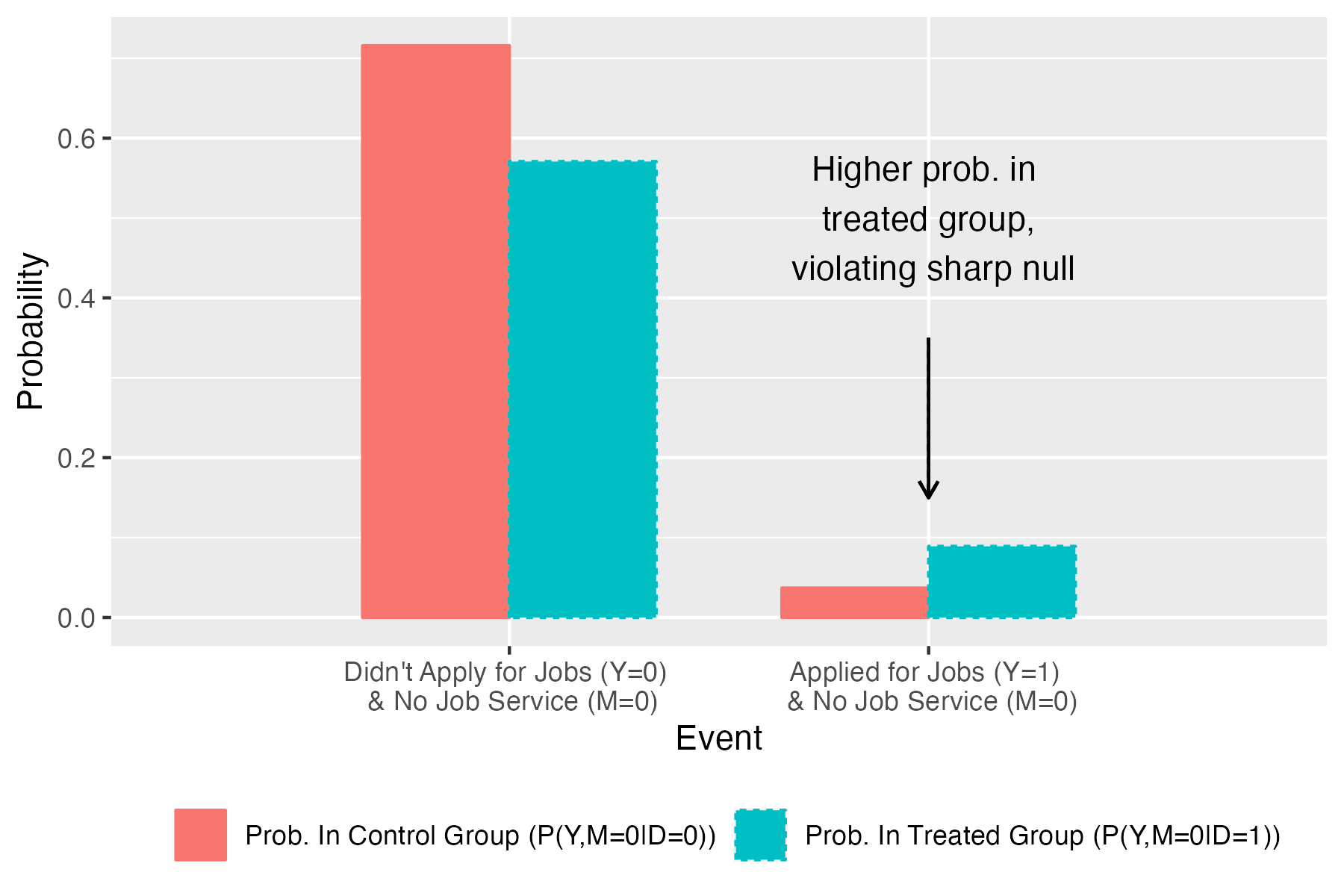
Appendix Figure 1: Illustration of Testable Implications in bursztyn_misperceived_2020 Using Full Sample

appendixfigure]fig:bursztyn_bin_appendix Note: This figure is analogous to Figure 1 except it uses the full sample rather than restricting to men who initially underestimate others’ beliefs.

Alternative tests.

In the main text, we report statistical tests of the sharp null using CS. LABEL:tbl:pvals reports analogous test results using the tests of ARP and FSST. The qualitative pattern across the tests is similar. One notable difference is that we do not reject the null for the relationship-quality mechanism in baranov_maternal_2020 using ARP, although this is perhaps unsurprising given the low power of ARP in simulations calibrated to this mechanism.

Application	M	CS	ARP	FSSTdd	FSSTndd
Bursztyn et al (main sample)	Job-search Sign-up	$0.020$	$0.030$	$0.018$	$0.018$
Bursztyn et al (full sample)	Job-search Sign-up	$0.019$	$0.020$	$0.019$	$0.019$
Baranov et al	Grandmother	$0.023$	$0.030$	$0.011$	$0.015$
Baranov et al	Relationship	$0.028$	$0.650$	$0.037$	$0.049$
Baranov et al	Grandmother + Relationship	$0.654$	$0.550$	$0.115$	$0.256$

Appendix Table 3: $p$-values for tests for the sharp null using alternative procedures

appendixtable]tbl:pvals

References

- (1)
- Andrews et al. (2023) Andrews, Isaiah, Jonathan Roth, and Ariel Pakes, “Inference for Linear Conditional Moment Inequalities,” The Review of Economic Studies, January 2023, p. rdad004.
- Angel and Spinka (2021) Angel, Omer and Yinon Spinka, “Pairwise optimal coupling of multiple random variables,” May 2021. arXiv:1903.00632 [math].
- Angrist and Hull (2023) Angrist, Joshua D. and Peter Hull, “Instrumental variables methods reconcile intention-to-screen effects across pragmatic cancer screening trials,” Proceedings of the National Academy of Sciences, December 2023, 120 (51), e2311556120. Publisher: Proceedings of the National Academy of Sciences.
- Angrist et al. (2023) , Parag A. Pathak, and Roman A. Zarate, “Choice and consequence: Assessing mismatch at Chicago exam schools,” Journal of Public Economics, July 2023, 223, 104892.
- Balke and Pearl (1997) Balke, Alexander and Judea Pearl, “Bounds on Treatment Effects from Studies with Imperfect Compliance,” Journal of the American Statistical Association, September 1997, 92 (439), 1171–1176. Publisher: Taylor & Francis _eprint: https://doi.org/10.1080/01621459.1997.10474074.
- Baranov et al. (2020) Baranov, Victoria, Sonia Bhalotra, Pietro Biroli, and Joanna Maselko, “Maternal Depression, Women’s Empowerment, and Parental Investment: Evidence from a Randomized Controlled Trial,” American Economic Review, March 2020, 110 (3), 824–859.
- Borusyak (2015) Borusyak, Kirill, “Bounding the Population Shares Affected by Treatments,” March 2015.
- Bursztyn et al. (2020) Bursztyn, Leonardo, Alessandra L. González, and David Yanagizawa-Drott, “Misperceived Social Norms: Women Working Outside the Home in Saudi Arabia,” American Economic Review, October 2020, 110 (10), 2997–3029.
- Charnes and Cooper (1962) Charnes, A. and W. W. Cooper, “Programming with linear fractional functionals,” Naval Research Logistics Quarterly, 1962, 9 (3-4), 181–186. _eprint: https://onlinelibrary.wiley.com/doi/pdf/10.1002/nav.3800090303.
- Cho and Russell (2023) Cho, JoonHwan and Thomas M. Russell, “Simple Inference on Functionals of Set-Identified Parameters Defined by Linear Moments,” May 2023. arXiv:1810.03180 [econ].
- Cox and Shi (2022) Cox, Gregory and Xiaoxia Shi, “Simple Adaptive Size-Exact Testing for Full-Vector and Subvector Inference in Moment Inequality Models,” The Review of Economic Studies, March 2022, p. rdac015.
- Deuchert et al. (2019) Deuchert, Eva, Martin Huber, and Mark Schelker, “Direct and Indirect Effects Based on Difference-in-Differences With an Application to Political Preferences Following the Vietnam Draft Lottery,” Journal of Business & Economic Statistics, October 2019, 37 (4), 710–720. Publisher: Taylor & Francis _eprint: https://doi.org/10.1080/07350015.2017.1419139.
- D’Haultfœuille et al. (2024) D’Haultfœuille, Xavier, Stefan Hoderlein, and Yuya Sasaki, “Testing and relaxing the exclusion restriction in the control function approach,” Journal of Econometrics, March 2024, 240 (2), 105075.
- Fang and Santos (2019) Fang, Zheng and Andres Santos, “Inference on Directionally Differentiable Functions,” The Review of Economic Studies, January 2019, 86 (1), 377–412.
- Fang et al. (2023) , , Azeem M. Shaikh, and Alexander Torgovitsky, “Inference for Large-Scale Linear Systems With Known Coefficients,” Econometrica, 2023, 91 (1), 299–327. _eprint: https://onlinelibrary.wiley.com/doi/pdf/10.3982/ECTA18979.
- Flores and Flores-Lagunes (2010) Flores, Carlos and Alfonso Flores-Lagunes, “Nonparametric Partial Identification of Causal Net and Mechanism Average Treatment Effects,” Working paper January 2010.
- Frangakis and Rubin (2002) Frangakis, Constantine E. and Donald B. Rubin, “Principal Stratification in Causal Inference,” Biometrics, March 2002, 58 (1), 21–29.
- Frölich and Huber (2017) Frölich, Markus and Martin Huber, “Direct and Indirect Treatment Effects–Causal Chains and Mediation Analysis with Instrumental Variables,” Journal of the Royal Statistical Society Series B: Statistical Methodology, November 2017, 79 (5), 1645–1666.
- Huber (2019) Huber, Martin, “A review of causal mediation analysis for assessing direct and indirect treatment effects,” Technical Report 2019.
- Huber and Mellace (2015) and Giovanni Mellace, “Testing Instrument Validity for Late Identification Based on Inequality Moment Constraints,” The Review of Economics and Statistics, 2015, 97 (2), 398–411. Publisher: The MIT Press.
- Huber et al. (2017) , Lukas Laffers, and Giovanni Mellace, “Sharp IV Bounds on Average Treatment Effects on the Treated and Other Populations Under Endogeneity and Noncompliance,” Journal of Applied Econometrics, 2017, 32 (1), 56–79. _eprint: https://onlinelibrary.wiley.com/doi/pdf/10.1002/jae.2473.
- Imai et al. (2010) Imai, Kosuke, Luke Keele, and Teppei Yamamoto, “Identification, Inference and Sensitivity Analysis for Causal Mediation Effects,” Statistical Science, February 2010, 25 (1), 51–71. Publisher: Institute of Mathematical Statistics.
- Kitagawa (2015) Kitagawa, Toru, “A Test for Instrument Validity,” Econometrica, 2015, 83 (5), 2043–2063. _eprint: https://onlinelibrary.wiley.com/doi/pdf/10.3982/ECTA11974.
- Lee (2009) Lee, David S., “Training, Wages, and Sample Selection: Estimating Sharp Bounds on Treatment Effects,” The Review of Economic Studies, July 2009, 76 (3), 1071–1102.
- Ludwig et al. (2011) Ludwig, Jens, Jeffrey R Kling, and Sendhil Mullainathan, “Mechanism Experiments and Policy Evaluations,” Journal of Economic Perspectives, August 2011, 25 (3), 17–38.
- Miles (2023) Miles, Caleb H, “On the causal interpretation of randomised interventional indirect effects,” Journal of the Royal Statistical Society Series B: Statistical Methodology, September 2023, 85 (4), 1154–1172.
- Mourifié and Wan (2017) Mourifié, Ismael and Yuanyuan Wan, “Testing Local Average Treatment Effect Assumptions,” The Review of Economics and Statistics, May 2017, 99 (2), 305–313.
- Pearl (2001) Pearl, Judea, “Direct and indirect effects,” in “Proceedings of the Seventeenth Conference on Uncertainty in Artificial Intelligence” San Francisco 2001, pp. 411–420.
- Robins and Greenland (1992) Robins, James M. and Sander Greenland, “Identifiability and Exchangeability for Direct and Indirect Effects,” Epidemiology, 1992, 3 (2), 143–155. Publisher: Lippincott Williams & Wilkins.
- Sun (2023) Sun, Zhenting, “Instrument Validity for Heterogeneous Causal Effects,” June 2023. arXiv:2009.01995 [econ, math, stat].
- VanderWeele (2012) VanderWeele, Tyler J., “Comments: Should Principal Stratification Be Used to Study Mediational Processes?,” Journal of research on educational effectiveness, July 2012, 5 (3), 245–249.
- VanderWeele (2016) , “Mediation Analysis: A Practitioner’s Guide,” Annual Review of Public Health, 2016, 37, 17–32.
- Villani (2009) Villani, Cédric, Optimal Transport, Vol. 338 of Grundlehren der mathematischen Wissenschaften, Berlin, Heidelberg: Springer, 2009.
- Wang et al. (2017) Wang, Linbo, James M. Robins, and Thomas S. Richardson, “On falsification of the binary instrumental variable model,” Biometrika, March 2017, 104 (1), 229–236.
- Zhang and Rubin (2003) Zhang, Junni L. and Donald B. Rubin, “Estimation of Causal Effects via Principal Stratification When Some Outcomes are Truncated by “Death”,” Journal of Educational and Behavioral Statistics, December 2003, 28 (4), 353–368. Publisher: American Educational Research Association.