On Machine Learning Complete Intersection Calabi-Yau $3$-folds

Kaniba Mady Keita

Centre de Calcul de Modélisation et de Simulation: CCMS

Department of Physics, Faculty of Sciences and Techniques, University of Sciences, Techniques and Technologies of Bamako, FST-USTTB, BP:E3206, Mali.

Abstract

Gaussian Process Regression, Kernel Support Vector Regression, the random forest, extreme gradient boosting and the generalized linear model algorithms are applied to data of Complete Intersection Calabi-Yau $3$-folds. It is shown that Gaussian process regression is the most suitable for learning the Hodge number $h^{2,1}$ in terms of $h^{1,1}$. The performance of this regression algorithm is such that the Pearson correlation coefficient for the validation set is $R^{2}=0.9999999995$ with a Root Mean Square Error $RMSE=0.0002895011$. As for the calibration set, these two parameters are as follows: $R^{2}=0.9999999994$ and $RMSE=0.0002854348$. The training error and the cross-validation error of this regression are $1\times 10^{-9}$ and $1.28\times 10^{-7}$, respectively. Learning the Hodge number $h^{1,1}$ in terms of $h^{2,1}$ yields $R^{2}=1.000000$ and $RMSE=7.395731\times 10^{-5}$ for the validation set of the Gaussian Process regression.

1 Introduction

String theory is presently known as a powerful candidate of quantum gravity. However, consistency of string theory requires $26$-dimension Minkowski spacetime for bosonic string, $10$-dimension Minkowski spacetime for (type I, type IIA, type IIB, heterotic) superstrings and supergravities theories. It is also true that $11$ is the critical dimension for $M$-theory. Besides these critical dimensions, anomaly cancellation of the ten-dimensional superstrings theories requires the gauge group to be $SO(32)$ or $E_{8}\times E_{8}$ [1]. To make contact with a potential $4$-dimensional Minkowski spacetime effective field theory, one must hence compactify the remaining $6$-dimensional manifold in a very special way. The simplest approach is to consider the following vacuum form for the ten-dimensional spacetime.

$$\mathfrak{M^{10}}=\mathfrak{M^{4}}\times\textsl{X}^{6}$$ (1.1)

where $\mathfrak{M^{4}}$ is the usual four-dimansional Minkowski spacetime and $\textsl{X}^{6}$ is a compactified internal manifold.

Phenomenologically, interesting scenarios arrived when the $E_{8}\times E_{8}$ heterotic string is compactified on a Calabi-Yau three-fold. This is the outcome of requiring an unbroken $\mathcal{N}=1$ supersymmetry effective action in the (3+1)-dimensional Minkowski spacetime [2]. Additionally, the compactification of the type IIA or type IIB theories on a Calabi-Yau $3$-fold yields $\mathcal{N}=2$ supersymmetry effective action in the (3+1)-dimensional Minkowski spacetime. The overall conclusion is that compactifying superstring theory on a Calabi-Yau $n$-fold breaks $\frac{3}{4}$ of the original supersymmetry [4, 5, 6]. These results give Calabi-Yau manifolds a very special position as far as one is considering the compactification of string theory in its various forms. The key outcome is that the physics of $\mathfrak{M^{4}}$ is determined by the geometry of $\textsl{X}^{6}$ [7].

Calabi-Yau manifolds (complete intersection Calabi-Yau, CICY ) are by now understood partially. For instance, $\text{CICY}_{n}$ have a defining configuration matrix, a defining Hodge diamond characterized by Hodge numbers $h^{p,q},(p,q=1,2,3,....)$, the intersection number $d_{rst}\left(r,s,t=1,2,...,h^{1,1}\right)$ and the first Pontrjagin class $p_{1}(T\textsl{X}^{6})$ of the tangent bundle [7]. The Hodge numbers $h^{p,q}$ are the dimensions of the Dolbeault cohomology group of CICY. As far as $\text{CICY}_{3}$ are concerned, one is left with $h^{1,1}$ and $h^{2,1}$ unspecified. These numbers do not uniquely define the manifold in question, although. There are moduli deformations (changes of shape and size) that do not affect the topology of $\text{CICY}_{3}$. The Hodge number $h^{2,1}$ for instance, represents the number of deformation in the complex structure (shape) of the Calabi-Yau manifold in question. In brief, in any Calabi-Yau manifold, there are basically, $h^{2,1}$-parameter family of topologically equivalent varieties distinct just by complex structures. On the other hand, $h^{1,1}$ is the number of Kh$\ddot{a}$hler-structure (size) deformation changes of $\text{CICY}_{3}$. These manifolds have the same topology but different shapes or sizes. The pairs $\left(h^{1,1},\,h^{2,1}\right)$ are therefore a natural playground for applying machine learning techniques.

The application of techniques from machine learning (ML) in analyzing aspects of CICY is nowadays very productive [8, 9, 10, 11, 12, 13, 14]; we refer to these articles and references therein for further information. In these approaches, classification and regression which can be both supervised and unsupervised are used. In ref.[15], the enterprise of using ML to address issues of Calabi-Yau manifolds has been put forward. This author gave winning evidence of the utility of machine learning in addressing issues of CICY. The main interests in these computations are using classification or regression techniques to learn the Hodge numbers $h^{p,q}$ when the configuration matrices are taken as the input of the algorithms [16, 17, 18, 19, 20]. Several models have been utilized in this prelude and we are learning that most of these models are performing well on the dataset of $\text{CICY}_{3}$ and $\text{CICY}_{4}$. Using configuration matrix as an input is surely a troublesome approach and it might greatly affect the performance of the model-building due to the ambiguities of its definition. This can explain somehow the bad performance in learning $h^{3,1}$ of the deep multi-task approach in [20]. Machine learning of matrix manipulation is not also well understood as of today. Changing two rows or two columns of a matrix does not affect the key properties of that matrix. This operation; however, has far-reaching consequences as far as CICY is concerned [3].

The main goal of this manuscript is to avoid this plan of attack. In doing so, we consider one of the Hodge numbers as an input and machine learn the other one. In other word, we learn the Hodge number $h^{2,1}$ in term of $h^{1,1}$. This is a very interesting problem; the two numbers represent the number of vector multiplets ($h^{1,1}$) and the number of hypermultiplets ($h^{2,1}+1$) as far as the IIA string theory is compactified on a Calabi-Yau manifold [4].

The shape and the size of a manifold are naturally related; the primary objective of this article is to access the nature of this connection for $\text{CICY}_{3}$. This is the domain of the regression techniques in machine learning and there are several algorithms to this end. In this work, we will apply Gaussian Process Regression (gausspr) [21], Kernel Support Vector Regression (KSVM) [22, 23, 24], the random forest (RF) [25, 26], extreme gradient boosting (xgboost) [27] and the generalized linear model (Glm) [28]. A comparative study of the performance of these regressions is discussed in this paper. We also conduct a clustering of CICY into three groups. This is an alternative way of studying CICY by ML. Our results supply supporting facts about the usefulness of ML in dealing with $\text{CICY}_{3}$. The remaining parts of this paper are divided as follows: In the next section, facts on CICY and aspects of string compactification on a CICY are presented. Section $3$ is devoted to regressions algorithms for learning $h^{2,1}$ in terms of $h^{1,1}$ and we describe the hyperparameters of the chosen regressions. The results of these regressions apply to $\text{CICY}_{3}$ are laid out and discussed in section $5$. The last section is consecrated to the conclusion and the possible extension of this work.

2 Complete Intersection Calabi-Yau Manifolds and String compactification

Understanding the structure of the internal manifold in superstring compactification is of capital importance in string theory. Special attentions have been paid to the study of CICY. Hence, we begin with the presentation of some useful concepts about $\text{CICY}_{n}$ which will be followed by an overview of string compactification on these manifolds. It is interesting to note that this Calabi-Yau compactification is phenomenologically very instructive and attractive.

2.1 Facts about Complete Intersection Calabi-Yau Manifolds: CICY

In this subsection, we review the basic concepts of CICY. The standard references of what we will highlight are refs.[29, 30, 3, 32, 33]. The basic properties of CICY have been derived in those papers. First of all, let the ambiant space $\mathbb{M}=\mathbb{P}_{1}^{n_{1}}\times\mathbb{P}_{2}^{n_{2}}\times...\times\mathbb{P}_{m}^{n_{m}}$ be a product of $m$ complex projective spaces of complex dimensions $n_{i}$, respectively. In addition, let $\mathcal{P}^{\alpha}\left(z^{\mu}\right),\quad\left(\alpha=1,2,...,K\right)$ be $K$ homogeneous holomorphic polynomial such that if $z_{r}^{\mu}$ is the homogeneous coordinates of $\mathbb{P}_{r}^{n_{r}}$, then $\mathcal{P}^{\alpha}\left(\lambda z_{r}^{\mu}\right)=\lambda^{q^{r}_{\alpha}}\mathcal{P}^{\alpha}\left(z_{r}^{\mu}\right)$. The sets $q^{r}_{\alpha}$ are called the homogeneous degrees of the polynomial $\mathcal{P}^{\alpha}\left(z^{\mu}\right)$ with respect to the coordinates of $\mathbb{P}_{r}^{n_{r}}$. Finally, let $\mathcal{X}^{\alpha}:\mathcal{P}^{\alpha}\left(z^{\mu}\right)=0$ be the zero locus of $\mathcal{P}^{\alpha}\left(z^{\mu}\right)$, then we have the following fact.

$\mathbf{Fact1:}$ The manifold $\mathbb{X}=\mathcal{X}^{1}\cap\mathcal{X}^{1}\cap\mathcal{X}^{2}\cap....\cap\mathcal{X}^{K}\subset\mathbb{M}$ (which is a complete interection of the hypersurfaces $\mathcal{X}^{\alpha}$) is a Calabi-Yau manifold if and only if we have

$$\sum_{\alpha=1}^{K}q^{r}_{\alpha}=n_{r}+1,\quad r=1,...,m.$$ (2.1)

These concepts about a CICY can be encoded into the so-called $\it{Configuration\,Matrix}$ denoted by

$$\mathbb{X}=\left[\begin{array}[]{c||ccc}\mathbb{P}^{n_{1}}&q^{1}_{1}&\cdots&q^{1}_{K}\\ \mathbb{P}^{n_{2}}&q^{2}_{1}&\cdots&q^{2}_{K}\\ \vdots&\vdots&\ddots&\vdots\\ \mathbb{P}^{n_{m}}&q^{m}_{1}&\cdots&q^{m}_{K}\\ \end{array}\right]\qquad=\left[\begin{array}[]{c||ccc}n_{1}&q^{1}_{1}&\cdots&q^{1}_{K}\\ n_{2}&q^{2}_{1}&\cdots&q^{2}_{K}\\ \vdots&\vdots&\ddots&\vdots\\ n_{m}&q^{m}_{1}&\cdots&q^{m}_{K}\\ \end{array}\right],\quad q^{r}_{a}\in\mathbb{Z}_{\geq 0}.$$ (2.2)

The dimension of the CICY manifold $\mathbb{X}$ is derived from the equation ( 2.3).

$$\sum_{r=1}^{m}n_{r}=dim_{\mathbb{C}}\mathbb{X}+K.$$ (2.3)

The equation (2.1) along with (2.3) signal the finiteness of $\text{CICY}_{n}$ for any $n$. More importantly, the Hodge numbers can be derived from the $\it{configuration\,matrix}$ [29, 30, 31, 3, 32].

$\mathbf{Fact2:}$ The number of $\text{CICY}_{n}$ is finite due to the equations (2.1) and (2.3). For instance, by considering one single complex projective space $\mathbb{P}^{n}$ and $K$ polynomials intersecting on it, we have:

$$n=dim_{\mathbb{C}}\mathbb{X}+K\quad\text{and}\quad\sum_{\alpha=1}^{K}q^{r}_{\alpha}=n+1\quad\text{implying\,\,that}\quad\sum_{\alpha=1}^{K}q^{r}_{\alpha}=dim_{\mathbb{C}}\mathbb{X}+K+1.$$ (2.4)

As an illustration, for $dim_{\mathbb{C}}\mathbb{X}=4$ and $K=1$, one gets $(n,\,q)=(5,\,6)$; this manifold is denoted by $\left[5||6\right]$. In the same case for $K=2$, one may get $\left[6||3\,4\right]$ and $\left[6||2\,5\right]$. In these examples, we are requiring that $q^{r}_{\alpha}\geq 2$. The Fermat quintic equation in $\mathbb{P}^{4}$ denoted by $\left[4||5\right]$ as well as the solution space for the intersection of a quartic and a quadratic in $\mathbb{P}^{5}$, $\left[5||4\,2\right]$, are interesting examples of $\text{CICY}_{3}$. More importantly, the quotient of the Tian-Yau manifold [34, 35] (2.5) by a freely acting $\mathbb{Z}_{3}$ is of capital interest in $\text{CICY}_{3}$ compactification. It corresponds to three generations of particles, which is an interesting result [36, 37, 38]. Note that the Tian-Yau manifold itself is an example of noncompact CICY $3$-folds. Nevertheless, the quotient of the Tian-Yau manifold by a freeling acting $\mathbb{Z}_{3}$ is a compact $3$-fold.

$$\mathbb{X}_{TY}=\left[\begin{array}[]{c||ccc}3&1&3&0\\ 3&1&0&3\\ \end{array}\right]$$ (2.5)

Most of the interesting manifolds are obtained by taking the quotient of a manifold of $SU(3)$ holonomy by one of its discrete freely acting symmetry groups.

$\mathbf{Fact3:}$ For any $\text{CICY}_{n}$ the Hodge number $h^{p,q}$ satisfy the complex conjugation and the Hodge $*$ or Poincaré duality:

$$h^{p,\,q}=h^{q,\,p}\quad\text{and}\quad h^{n-p,\,n-q}=h^{p,\,q}$$ (2.6)

Using these properties, one easily finds that the only unspecified Hodge numbers for $\text{CICY}_{3}$ are $h^{1,1}$ and $h^{2,1}=h^{1,2}$. The Euler characteristic $\chi$ of any $\text{CICY}_{3}$ is then given by the formula

$$\chi=2\left(h^{1,\,1}-h^{2,\,1}\right)$$ (2.7)

2.2 String Compactification on a Calabi-Yau Manifold

Having presented a few facts about Calabi-Yau complete intersections, we are now in a position to proceed by looking at string compactification on these manifolds. The standard references on this aspect are refs.[2, 4, 5, 6, 39, 40]. We will start by reviewing aspects of string compactification that are relevant for $\text{CICY}_{3}$ manifolds. This restriction does not alter the conclusion of this manuscript as far as the dataset of $\text{CICY}_{3}$ is concerned. When various string theories are compactified on a $\text{CICY}_{3}$, one finds an interesting four-dimensional theory with $\mathcal{N}=2$ supersymmetry.

The four-dimensional with $\mathcal{N}=2$ supersymmetry, from the compactification of superstring theory on a Calabi-Yau manifold three-folds has interesting aspects. For instance, the $\mathcal{N}=2$ supermultiplets is divided into abelian vector multiplets and hypermultiplets. For IIA and IIB strings compactification on a $\text{CICY}_{3}$, the numbers of these multiplets are given in Table 1.

Table 1: The division of $\mathcal{N}=2$ supermultiplets

String compactified on a $\text{CICY}_{3}$	$\mathcal{N}=2$ supermultiplets
type	vector multiplets	hypermultiplets
IIA	$h^{1,1}$	$h^{2,1}$+1
IIB	$h^{2,1}$	$h^{1,1}$+1

If two $\text{CICY}_{3}$ $\mathbb{X}^{1}$ and $\mathbb{X}^{2}$ are such that $h^{1,1}\left(\mathbb{X}^{1}\right)=h^{2,1}\left(\mathbb{X}^{2}\right)$, then the manifolds $\mathbb{X}^{1}$ and $\mathbb{X}^{2}$ are said to be mirror. One immediate consequence of (Table.1) is that type IIA superstring theory compactified on $\mathbb{X}^{1}$ is equivalent to type IIB superstring theory compactified on $\mathbb{X}^{2}$. The mirror symmetry also implies the self-duality nature of the space o string theory vacua. The implication of mirror symmetry in what to follow is an implicit connection between learning $h^{2,1}$ in terms of $h^{1,1}$ and learning $h^{1,1}$ in terms of $h^{2,1}$. One natural intent of this manuscript is to clarify this issue.

Upon compactification of the $E_{8}\times E_{8}$ heterotic string on a $\text{CICY}_{3}$ a few things happen. The most noticeable is that one of the $E_{8}$ is broken to $E_{6}$ with the following decomposition of its $248$-dimensional representation as:

$$E_{8} \longrightarrow SU(3)\times E_{6}$$

$$248 \longrightarrow (1,\,78)\oplus(3,\,27)\oplus(\bar{3},\,\bar{27})\oplus(8,\,1)$$ (2.8)

From the decomposition (2.2), we are thus able to put all the massless fields into the $27$ representation of $E_{6}$ by using a grand unification theory based on $E_{6}$. The generation one gets is half the Euler characteristic of the Calabi-Yau manifold [2, 29]. This outcome is generally true for any Calabi-Yau compactification of the heterotic string theory.

3 Regressions Algorithms for Learning $h^{2,1}$ in terms of $h^{1,1}$

The basic purpose of regression algorithms is to find the best hypothesis function $\mathcal{f}$ which relates some input values to the output ones [41]. When the input is one variable as in our case, then the regressions are called uni-variate or simple. This is in contrast to multivariate regression scenarios. The regression can be either linear or nonlinear depending on the nature of the function $\mathcal{f}$ used. In this work, we model our regressions by the formula given by

$$\hat{h}^{2,1}=\mathcal{f}\left(h^{1,1}\right)$$ (3.1)

where the output of the regression, the predicted value, is $\hat{h}^{2,1}$ and the target output is $h^{2,1}$. The error of the predictions is the difference between the true target value $h^{2,1}$ and predicted target value $\hat{h}^{2,1}$. The relationship (3.1) is known as a simple regression in contrast to multiple regression or multivariate regression. The true value $h^{2,1}$ is related to the model prediction $\hat{h}^{2,1}$ by the relation

$$h^{2,1}=\hat{h}^{2,1}+\epsilon,\qquad\text{where}\,\,\epsilon\,\,\text{is\,the\,error}$$ (3.2)

Different approaches try to minimize the value of $\epsilon$ by using various minimization techniques. Before the application of the various regressions’ techniques, one has to divide the dataset into a train set ($80\%$) and a validation set ($20\%$). Sometimes, the data is separated into a train set, a validation set and a test set, but we will not follow this option in our work. The performance of a chosen model is measured by a few statistical parameters such as the mean square error (MSE), the root mean square error (RMSE), the mean absolute error (MAE), the Pearson correlation coefficient ($R^{2}$) and so on… One quantity that signals the underestimation (negative value of the bias) or overestimation (positive value of the bias) for the output by a given model is the bias. For these parameters, the formula is given in refs.[17, 41, 42]

MSE $$= \frac{1}{N}\sum_{i=1}^{N}\left(h^{2,1}_{i}-\hat{h}^{2,1}_{i}\right)^{2}$$

RMSE $$= \sqrt{MSE},$$

MAE $$= \frac{1}{N}\sum_{i=1}^{N}\left|h^{2,1}_{i}-\hat{h}^{2,1}_{i}\right|$$ (3.3)

$$R^{2} = 1-\frac{\sum_{i=1}^{N}\left(h^{2,1}_{i}-\hat{h}^{2,1}_{i}\right)^{2}}{\sum_{i=1}^{N}\left(h^{2,1}_{i}-\bar{h}^{2,1}\right)^{2}}$$

BIAS $$= \frac{1}{N}\sum_{i=1}^{N}\left(\hat{h}^{2,1}_{i}-h^{2,1}_{i}\right)$$

where in these equations, $N$ denotes the number of elements in the set (train set or validation set) under consideration and $\bar{h}^{2,1}$ represent the mean of $h^{2,1}$.

The best model must have the highest value for $R^{2}$ and the smallest value for the other parameters in the equation (3). To compute these parameters, we use the aforementioned algorithms which we will now outline in the remaining part of this section. The regression techniques use some parameters often called hyperparameters; the suitable values of these hyperparameters are also given.

3.1 The hyperparameters of the regressions techniques

The first regression technique we applied is the Gaussian Process Regression (gausspr). This is currently a famous regression technique used in the field of machine learning. The full theory goes beyond the scope of this manuscript. The necessary information about gausspr can be found in the references [43, 44]. In Gausspr one the hypothesis function is a Gaussian function and it is characterized by some hyperparameters. To implement the algorithm of Gausspr, we used the software R and the package kernlab [45]. The hyperparameters of gausspr are (var=0.15, kpar=automatic, cross-validation=5 and kernel=polydot); the list of hyper-parameters (kernel parameters) are abbreviated in kpar; the initial noise variance is denoted by var and finally tol represents the tolerance of termination criterion.

The second algorithm is the so-called kernel Support vector machine (KSVM). In this approach, one uses a kernel (function) to transform the data points into a feature space. Then, an $\epsilon$-insensitive error function is defined to form a hyperplane within the feature space. The data points which lie on the hyperplanes are called the support vectors. Again, the full mathematics are omitted and can be consulted in ref.[43]. To implement KSVM, we also used R and the kernlab package. The hyperparameters used in KSVM are (kernel =polydot, kpar = automatic, C = 4, nu = 0.1, epsilon = 0.1, cross-validation = 0, cache = 40 and tol = 0.15); here nu sets the upper bound on the training error and the lower bound on the fraction of data points to become Support Vectors; C is the cost of constraints violation.

The next regression is random forest RF [25, 26] which uses the concepts of decision trees. For its implementation, we used the package randomforest [46]. Its basic parameters are the number of trees to grow (ntree=25); the number of variables randomly sampled as candidates at each split (mtry=2) and the minimum size of terminal nodes (nodesize=3).

The fourth regression applied is Extreme gradient boost (Xgboost). This is a very good regression algorithm. The package xgboost [47] has been used for its execution. It has two hyperparameters which are the max number of boosting iterations (nrounds=69) and the maximum depth of a tree (max-depth=3). The last regression does not have hyperparameters to set in. We are going to survey the data set of $\text{CICY}_{3}$ before the application of these techniques of regressions.

3.2 Data sets of $\text{CICY}_{3}$ and its Splitting into train and validation set

The complete data sets of $\text{CICY}_{3}$ is composed of 7890 different topological types of $\text{CICY}_{3}$. However, there are only 266 distinct pairs of $\left(h^{1,1},\,h^{2,1}\right)$. The plot of the Hodge number $h^{2,1}$ (H21) in function of $h^{1,1}$ (H11) are given in Figure 1. Several values of $h^{2,1}$ are mapped to a single value of $h^{1,1}$. Consequently, the machine learning of $h^{2,1}$ in term of $h^{1,1}$ is more challenging. This is virtually the same trouble one encounters in learning $h^{2,1}$ or $h^{1,1}$ by using the $\it{configuration\,matrices}$ as input of the algorithms. We divide the $7890$ $\text{CICY}_{3}$ into $6312$ ($80\%$) varieties used for training the models and $1578$ ($20\%$) manifolds for validating the algorithms.

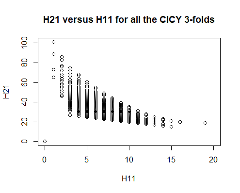
(a) H21 versus H11 for the 7890 CICY.

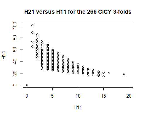
(b) H21 versus H11 for the 266 CICY

Figure 1: The plot of H21 versus H11.

4 Results and Discussions

The purpose of this section is to show the different results and discuss them in some detail. The first result is Table 2 which contains the values of the statistical parameters in equation (3) except the values of MAE.

Table 2: Few statistical Parameters of the applied regressions techniques

Regression	Validation			Calibration
	$R^{2}$	RMSE	BIAS	$R^{2}$	RMSE	BIAS
gausspr	0.9999999995	0.0002895011	3.754119E-6	0.9999999994	0.0002854348	-6.001535E-10
KSVM	0.9999982	0.3527558	0.3439119	0.9999980	0.3515819	0.3432654
RF	0.9984065	0.35785376	0.009894381	0.999977440	0.040472929	-0.000273553
Xgboost	0.7048157	4.7934372	-0.1547063	0.6921789	4.72444	2.958037E-7
Glm	0.5192372	6.123511	-0.07941958	0.4972947	6.037509	-1.163628e-13
PLS	0.5192372	6.1235110	-0.07941958	0.4972947	6.0375093	-7.490853E-16

In this table, we see that Gaussian process regression is the most powerful in terms of performance (lowest value of RMSE). It is then followed by the kernel support vector machine, the random forest, the extreme gradient boost and lastly by the generalized linear model. We surprisingly discovered that for the data set, the traditional partial least square (PLS) has more or less the same statistical parameters as the generalized linear model. One noticeable thing about Table 2 is that all of the applied techniques sure-estimate the value of the Hodge number $h^{2,1}$ for the validation set due to the value of the bias.

Next, we have the graphs of the calibration lines of gausspr in Figure 2 and KSVM in Figure 3. From these plots, it is visible that the two algorithms predicted precisely the Hodge number $h^{2,1}$. It is interesting to note that these regression techniques can be utilized to a great extent in the field of machine learning Calabi-Yau manifolds.

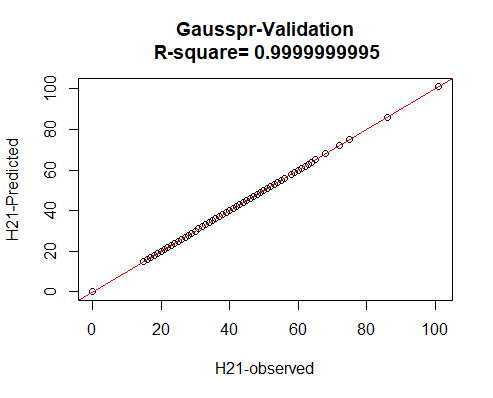
(a) gausspr for the validation set.

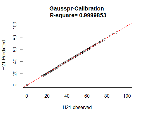
(b) Gausspr for the Calibration set

Figure 2: The predictions from Gausspr.

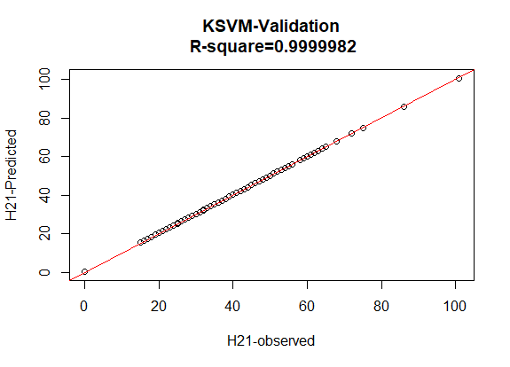
(a) KSVM for the validation set.

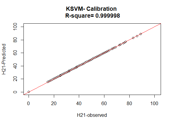
(b) KSVM for the calibration set

Figure 3: The predictions from Kernel Support Vector Machine.

The graphs for the regression lines of random forest and extreme gradient boost are depicted in Figure 4 and Figure 5, respectively.

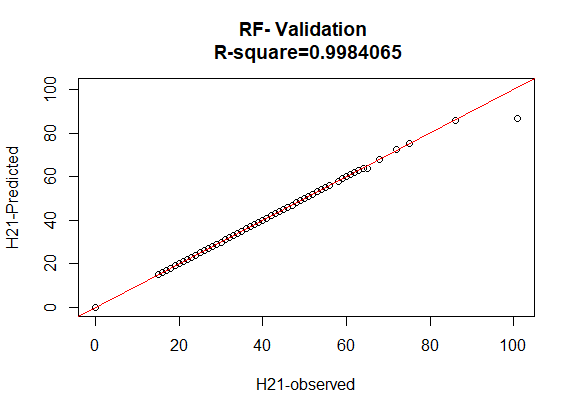
(a) RF for the validation set

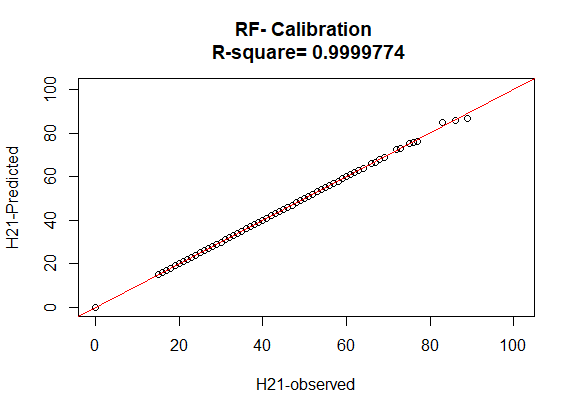
(b) RF for the calibration set

Figure 4: The predictions from the random forest.

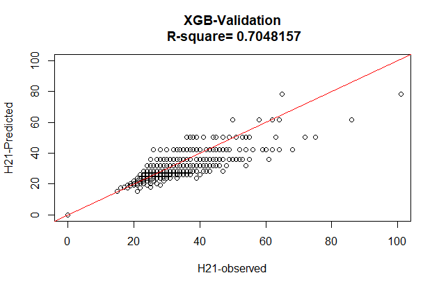
(a) Xgboost for the validation set

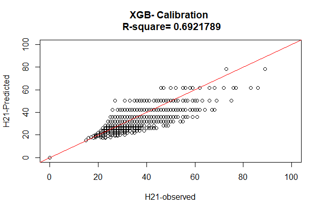
(b) Xgboost for the calibration set

Figure 5: The predictions from the extreme gradient boost.

We notice that random forest performs badly when the Hodge number $h^{2,1}$ is bigger. This is surely a knotty problem in the field of machine learning Calabi-Yau varieties. As for the predictions from extreme gradient boost, one observes that they are dispersed almost symmetrically around the regression line. The routes of this poor performance of extreme gradient boost are unclear to us. We therefore advise avoiding this regression algorithm in the field under consideration. It is certainly a very good minimization approach, but not in the flatland of machine learning of $\text{CICY}_{3}$. In stark contrast, however, we do have the superposition of the original and the predicted values of $h^{2,1}$ in Figure 6(a) which shows that the prediction is not as bad as it might first appear in Figure 5(a).

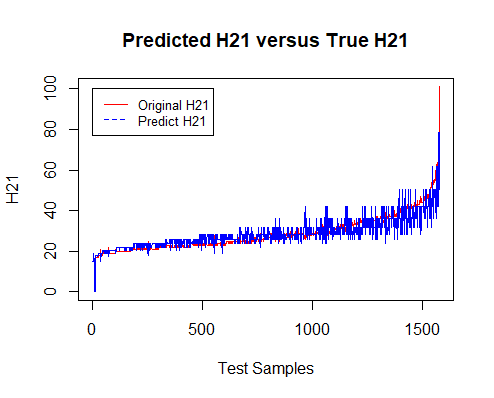
(a) For all the 7890 CICY.

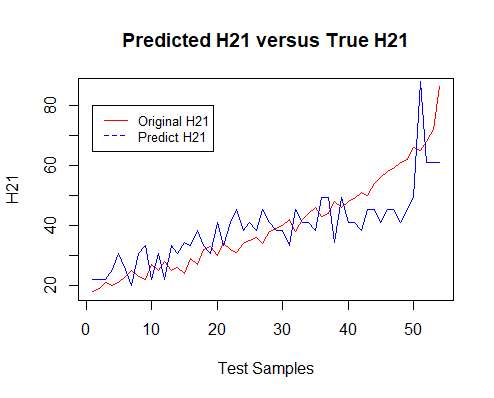
(b) The 266 CICY

Figure 6: The predictions superposed to its original values of $h^{2,1}$ from xgboost.

The last plots of the regression lines are the ones for the generalized linear model and the partial least square which are given in Figure 7 and Figure 8, respectively.

(a) Generalized Linear Model for the validation set.

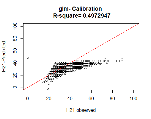
(b) Generalized Linear Model for the calibration

Figure 7: The predictions from the generalized linear model.

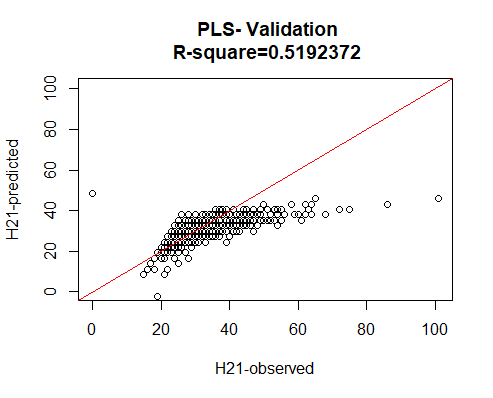
(a) Partial least square Model for the validation set.

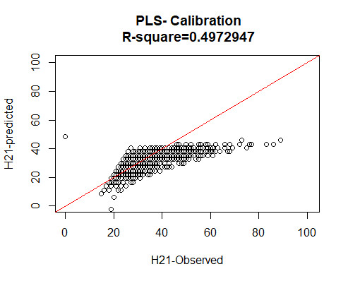
(b) Partial least square Model for the calibration

Figure 8: The predictions from the partial least square model.

These plots reveal that the glm and the pls models are definitely not suitable for addressing issues regarding application of machine learning of Calabi-Yau manifolds. Equally predictable is that the Xgboost, glm and pls are underestimating the values of the Hodge number $h^{2,1}$ which can be seen from the plots of the graphs of these models as well as in the values of their bias in Table 2 above.

In the field of machine learning, an important concept is the partitioning clustering of the data points into clusters. In this article, we apply three types of clustering: the k-means clustering, the Partitioning Around Medoids (PAM) clustering and the Clustering Large Applications (clara) method. The former is sensitive to outliers whereas pam is less sensitive to outliers. The figures of these clustering are shown in Figure 9 and Figure 10 below. In the jargon of data scientists, PAM is also known as K-Medoids clustering [48, 49]. Analyzing the usefulness of clustering $\text{CICY}_{3}$ into several groups and the physics associated to each group needs further probes and we postpone these investigations for future considerations. Notwithstanding, we detect a striking similarity between Figure 9(a) and Figure 9(b).

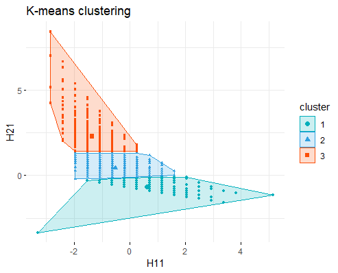
(a) K-mean clustering of the data points.

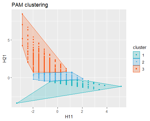
(b) Partitioning Around Medoids Clustering of the data point

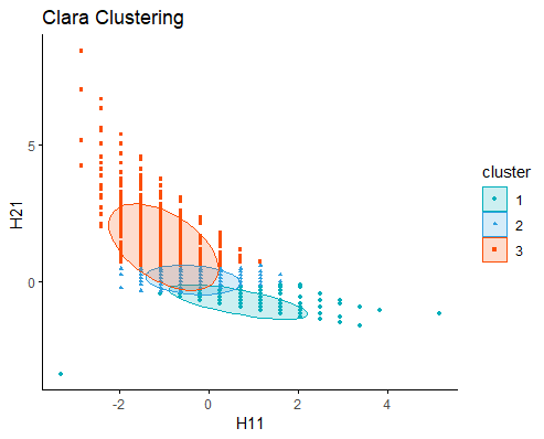
(c) Clustering Large Applications or Clara clustering

Figure 9: The three types of clustering of the data points.

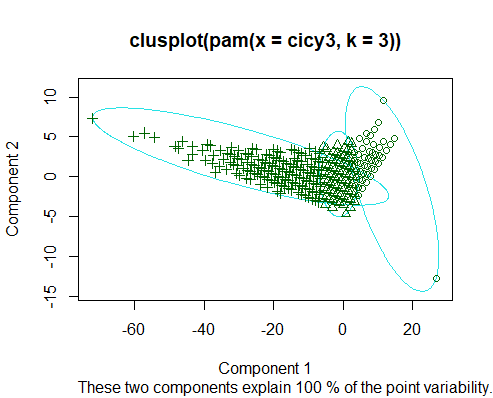
(a) the two components of pam clustering

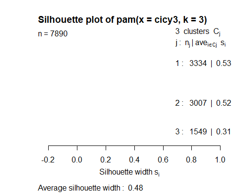
(b) The Silhouette plot of pam Clustering

Figure 10: Silhouette and Components plots of pam clustering

4.1 Regressions Techniques and the number of generations

In the context of Calabi-Yau compactification, the number of particle generations in the $four$-dimensional world is given by the relation [2].

$$\text{Number\, of\, Generation}=\frac{1}{2}\left|h^{1,1}-h^{2,1}\right|$$ (4.1)

Examples of Calabi-Yau manifolds having linear relations like equation (4.1) are scarce (one can look at for instance, Table $7\&9$ of [50]). In order to have $3$-generations in our regression models, we use equation (4.1) and the number of particle generations becomes

$$\text{Number\, of\, Generation}=\frac{1}{2}\left|h^{1,1}-\hat{h}^{2,1}\right|=3,\quad\text{implying\,that}\,\,\,\mathcal{f}\left(h^{1,1}\right)=h^{1,1}\pm 6$$ (4.2)

The number of generations from equation (4.2) are shown in Figure 11 and Figure 12.

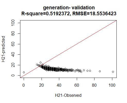
(a) Generation equation for the validation set.

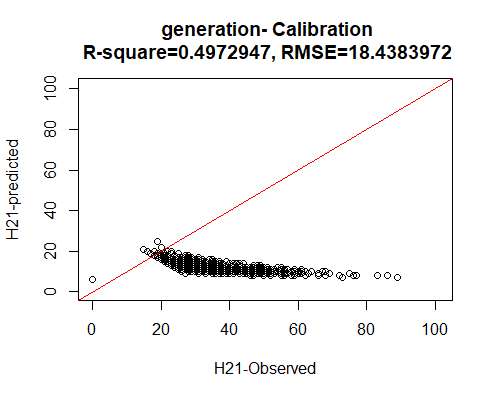
(b) Generation equation for the calibration

Figure 11: The predictions from $\mathcal{f}\left(h^{1,1}\right)=h^{1,1}+6$.

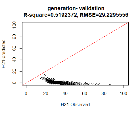
(a) generation two for the validation set.

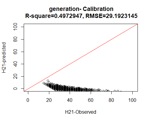
(b) generation two for the calibration

Figure 12: The predictions from $\mathcal{f}\left(h^{1,1}\right)=h^{1,1}-6$.

We observe that $h^{2,1}\approx\mathcal{f}\left(h^{1,1}\right)=h^{1,1}-6$ has to be avoid in equation (4.2). It is also evident from Figure 11 that $\text{CICY}_{3}$ having three generations are not so many.

Similar analysis can be carried out in replacing the $7890$ data sets of $\text{CICY}_{3}$ by the data sets of the $266$ distinct pairs of $\left(h^{1,1},\,h^{2,1}\right)$. The ($80\%$, $20\%$) division of the data set into the training sets and the validation sets results in $212$ samples for calibrating the models and $54$ samples for validating them. The statistical parameters for the above regressions are exposed in Table 3.

Table 3: Statistical Parameters for models applied to the $266$ $\text{CICY}_{3}$

Regression	Validation			Calibration
	$R^{2}$	RMSE	MAE	$R^{2}$	RMSE	MAE
gausspr	1.000000e+00	8.913495E-5	7.209163E-5	1.000000e+00	9.713904E-5	7.130115E-5
KSVM	0.9998109	0.6911974	0.5557933	0.9996605	0.7001122	0.5539415
RF	0.9883554	1.7488026	1.0432899	0.9888899	1.7384071	0.8420099
Xgboost	0.6094061	9.7423305	8.0058412	0.6355857	9.0960680	7.1641955
Glm	0.6084452	10.1644505	8.2209245	0.459558	11.077214	8.130806
PLS	0.6084452	10.1644505	8.2209245	0.459558	11.077214	8.130806

Not surprisingly, the order of performance for the regressions techniques remains the same. The most powerful one is always gausspr which is followed by KSVM. We then have RF at the third position in terms of performance. The plots of the regression lines of the validation sets for these three algorithms are depicted in Figure 13.

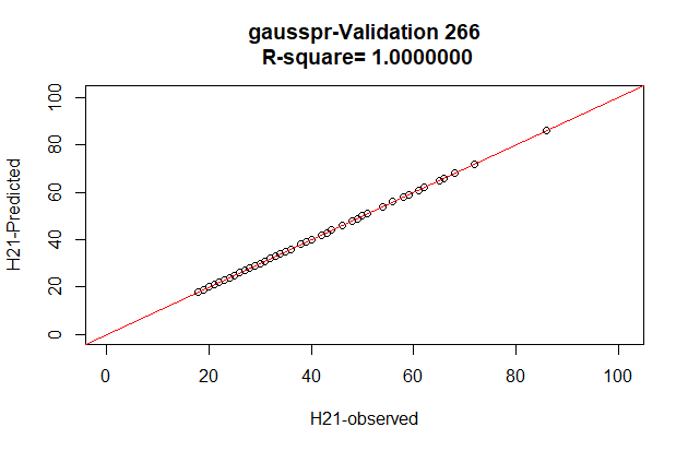
(a) gausspr for the set of 266 $\text{CICY}_{3}$

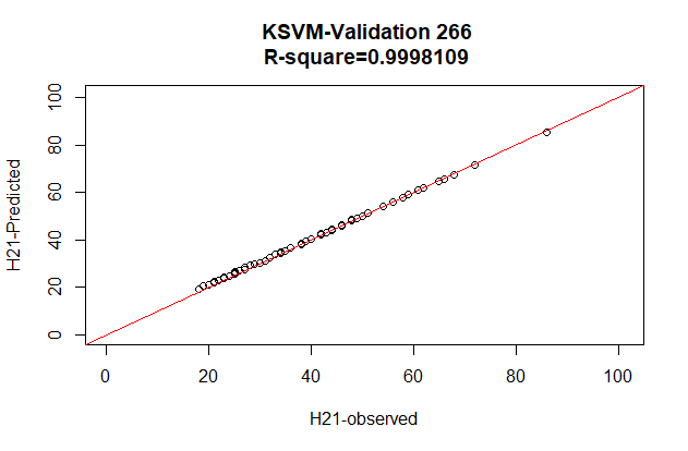
(b) KSVM for the set of 266 $\text{CICY}_{3}$

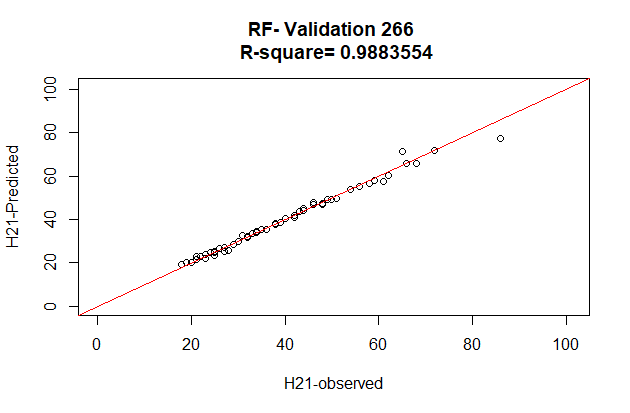
(c) RF for the validation set of 266 $\text{CICY}_{3}$

Figure 13: The predictions for the validation set of 266 $\text{CICY}_{3}$.

A glance at these figures reveals the excellent performance of these three regression techniques. It is apparent from Figure 13(c) that random forest has to be taken with caution when the values of $h^{2,1}$ is higher than $50$. These results resume the learning of $h^{2,1}$ as the output of the regressions when $h^{1,1}$ is taken as the input.

Likewise, one can instead take $h^{2,1}$ as the input of the algorithms and learn $h^{1,1}$ which is an interesting approach. The results for this option are resumed in Table 4 and in Figure 14.

Table 4: Few statistical Parameters for learning $h^{1,1}$ in terms of $h^{2,1}$

Regression	Validation			Calibration
	$R^{2}$	RMSE	BIAS	$R^{2}$	RMSE	BIAS
gausspr	1.000000e+00	7.395731E-5	6.503978E-7	1.000000e+00	7.540186E-5	9.016338E-11
KSVM	0.9999217	0.03692016	0.01780263	0.9999231	0.03759887	0.01803469
RF	0.9999994	0.001744083	7.604563E-5	0.999998	0.00314419	5.703422e-05
Xgboost	0.7529686	1.121953	-0.03815101	0.7359613	1.155875	-2.051232E-6
Glm	0.5192372	1.564346	-0.01375948	0.4972947	1.5949	-3.607428e-14

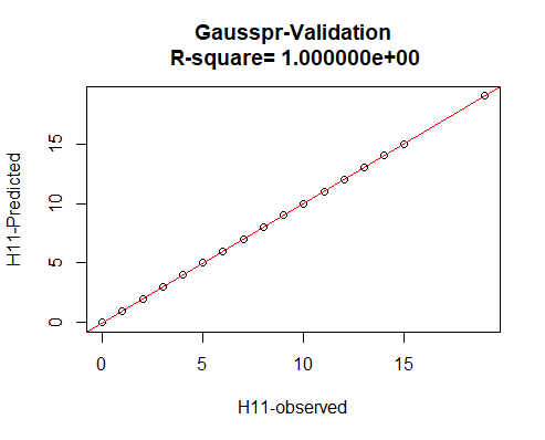
(a) gausspr for $h^{1,1}$ in terms of $h^{2,1}$

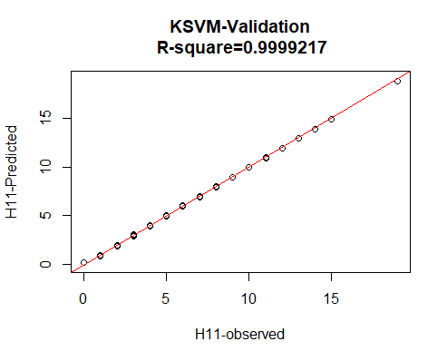
(b) KSVM for $h^{1,1}$ in terms of $h^{2,1}$

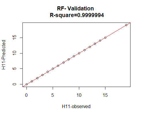
(c) RF for $h^{1,1}$ in terms of $h^{2,1}$

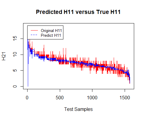
(d) Xgboost for $h^{1,1}$ in terms of $h^{2,1}$

Figure 14: The predictions for $h^{1,1}$ in terms of $h^{2,1}$

We see that this alternative way of machine learning Calabi-Yau manifolds is also possible in practice. More importantly, the performance order of the regression techniques remains unchanged.

5 Conclusions

In this paper, by using several regression techniques, we analyzed the data set of $780$ complete intersection Calabi-Yau manifolds of complex dimension three. First of all, we took the Hodge number $h^{1,1}$ as the input of the algorithms and machine learned the Hodge number $h^{2,1}$. The performance of these univariates regressions is measured by some statistical parameters which are reported on tables 2 and 3. We have also machine learned the Hodge number $h^{1,1}$ in terms of $h^{2,1}$ and the outcome is reported in table 4. By looking at the values of RMSE, one can see that Gaussian process regression is the suitable regression technique for the data sets of complete intersection Calabi-Yau $3$-folds. It is interesting to note that extreme gradient boost may encounter some issues when applied to $\text{CICY}_{3}$. The clustering into three groups of complete intersection of Calabi-Yau three folds is also carried out in this paper. This approach can be used to machine learn the $32$ families of $\text{CICY}_{3}$ having non-trivial torsion in integral cohomology group [51]. Similar analysis can be applied to the data set of complete intersection Calabi-Yau $four$-folds [20] and $five$-folds [13]. Our work can also be extended to analyze topological equivalent manifolds which is a challenging problem in itself [54].

By taking $h^{2,1}$ as the input of the algorithms, we remark that the classification of the regression techniques in terms of performance is not affected. This is not quiet surprising, since type IIA and type IIB string theories are related by dualities [52, 53].

Data Access Statement

The dataset used in this work is available in
https://www-thphys.physics.ox.ac.uk/projects/CalabiYau/cicylist/. We extracted the Hodge numbers from the text file.

References

- [1] M.B. Green and J.H. Schwarz, Caltech preprint 68-1182 (1984)
- [2] P. Candelas, Gary T. Horowitz, A. Strominger, E. Witten; Vacuum Configurations for Superstrings, Nucl. Phys. B 258 (1985) 46-74.
- [3] T. Hubsch, Calabi-Yau Manifolds: A Bestiary for Physicists, World Scientific, 1992, ISBN: 9810206623, 9789810206628.
- [4] Joseph Polchinski, String Theory Volume II, chapter 17.
- [5] M. B. Green, J. H. Schwarz & E. Witten, Superstring Theory, Volume 2: Loop amplitudes, Anomalies & Phenomenology, chapter 14-19.
- [6] Katrin Becker, Melanie Becker, and John H. Schwarz, String Theory and M-Theory: A Modern Introduction, chapter 9.
- [7] Yang-Hui He, The Calabi-Yau Landscape:from Geometry, to Physics, to Machine-Learning, arxiv: 1812:02893.
- [8] Wei Cui, Xin Gao,and Juntao Wang, Machine Learning on generalized Complete Intersection Calabi-Yau Manifolds, arXiv:2209.10157.
- [9] Harold Erbin, and Riccardo Finotello, Deep learning complete intersection Calabi-Yau manifolds, [arXiv:2311.11847 [hep-th]].
- [10] Anthony Ashmore, Yang-Hui He, and Burt Ovrut, Machine learning Calabi-Yau metrics, Fortsch.Phys. 68 (2020) 9, 2000068.
- [11] D. Aggarwal, Y.-H. He, E. Heyes, E. Hirst, H. N. S. Earp, and T. S. R. Silva, Machine-learning Sasakian and G2 topology on contact Calabi-Yau 7-manifolds, arXiv:2310.03064 [math.DG].
- [12] D. S. Berman, Y.-H. He, and E. Hirst, Machine learning Calabi-Yau hypersurfaces, Phys.Rev. D 105 no. 6, (2022) 066002, arXiv:2112.06350 [hep-th].
- [13] R. Alawadhi, D. Angella, A. Leonardo, T. Schettini Gherardini, Constructing and Machine Learning Calabi-Yau Five-folds, arXiv:2310.15966.
- [14] Rehan Deen, Yang-Hui He, Seung-Joo Lee and Andre Lukas, Machine learning string standard models, Phys. Rev. D 105, 046001 (2022).
- [15] Yang-Hui He, Deep-Learning the Landscape, arXiv:1706.02714.
- [16] Yang-Hui He and Andre Lukas, Machine learning Calabi-Yau four-folds, Phys.Lett.B 815 (2021) 136139.
- [17] F. Ruehle, Data science applications to string theory, Phys. Rep. 839 (2020) 1.
- [18] K. Bull, Y.H. He, V. Jejjala, and C. Mishra, Machine learning CICY threefolds, Phys.Lett. B 785 (2018) 65–72, arXiv:1806.03121.
- [19] H. Erbin and R. Finotello, Inception neural network for complete intersection Calabi-Yau 3-folds, Mach. Learn.: Sci. Technol. 2021, 2, 02LT03., arXiv:2007.13379.
- [20] Harold Erbin, Riccardo Finotello, Robin Schneider and Mohamed Tamaazousti, Deep multi-task mining Calabi–Yau four-folds, Mach. Learn.: Sci. Technol. 2022, 3 015006.
- [21] C.K.I. Williams and D. Barber, Bayesian classification with Gaussian processes, IEEE Transaction on Pattern Analysis and Machine Intelligence, 20 (12): 1342-1351, 1998, DOI: 10.1109/34.735807.
- [22] V Vapnik, The nature of Statistical learning theory, Springer, New York (1995).
- [23] Corinna Cortes and Vlafmir Vapnik, Support- Vector Networks, Machine Learning, 20, 273-297 (1995).
- [24] , H. Drucker, C. J. Burges, L. Kaufman, A. Smola and V. Vapnik, Support vector regression machines, Advances in Neural Information Processing Systems 9 (NIPS 1996).
- [25] Leo Breiman, Bagging predictors. Machine Learning, 6 (2), 123-140, 1996
- [26] Leo Breiman, Random Forests, Machine Learning, 45, 5-32, 2001.
- [27] J. Friedman, T. Hastie and R. Tinshirani, Additive logistic regression: a statistical view of boosting (with discussion and a rejoinder by the authors). Ann.Statist. 28 (April 2000) 337-407. DOI:10.1241/aos/1016218223.
- [28] McCulloch, Charles E., and Shayle R. Searle, Generalized, linear, and mixed models. John Wiley & Sons, 2004.
- [29] P.S. Green, T. H. Hubsch and C. A. Lutken, All the Hodge numbers for all Calabi-Yau complete intersections, Class.Quantum.Grav. 6 (1989) 105-124.
- [30] P. Candelas A.M. Dale C.A. Lutken, Complete Intersection Calabi-Yau Manifolds, Nucl.Phys. B 298 (1988) 493.
- [31] Anming He and Philip Candelas, On the Number of Complete Intersection Calabi-Yau Manifolds. Commun. Math. Phys. 135, 193-199 (1990).
- [32] T. Hubsch, Calabi-Yau Manifolds- Motivations and Constructions, Commun. Math. Phys. 108, 291-318 (1987).
- [33] Paul Green and Tristan Hubsch, Calabi-Yau Manifolds as Complete Intersections in Products of Complex Projective Spaces. Commun. Math. Phys. 109, 99-108 (1987).
- [34] G. Tian and S,-T. Yau, Complete Khhler manifolds with zero Ricci curvature. I. J. Amer. Math. Soc. 3 (1990), no. 3,579-609.
- [35] G. Tian and S,-T. Yau, Complete Khhler manifolds with zero Ricci curvature. II. Invent. Math. 106 (1991), no. 1,27-60.
- [36] P. Candelas and C.A. Lutken, Complete Intersection Calabi-Yau Manifolds. 2. Three Generation Manifolds, Nucl.Phys. B 306 (1988) 113.
- [37] P. Candelas, Yukawa Couplings for a Three Generation Superstring Compactification, Nucl. Phys. B 298 (1988) 357-368.
- [38] Rolf Schimmrigk, A New Construction of a Three Generation Calabi-Yau Manifold, Phys.Lett.B 193 (1987) 175.
- [39] , Doron GEPNER, Exactly Solvable String Compactifications on Manifolds of Holonomy, Phys. Lett. B 199 (3), (1987), 380-388.
- [40] J. H. SCHWARZ, The search for a realistic superstring vacuum. Phil. Trans. R. Soc. Lond. A 329,359-371, (1989).
- [41] Abhijit Ghatak, Machine Learning with R: Chapter 4. Springer Nature Singapore Pte Ltd. 2017.
- [42] Vijay Kotu and Bala Deshpande, Data Science: Concepts and Practice, Elsevier, ISBN: 978-0-12-814761-0, (2019).
- [43] Carl Edward Rasmussen and Christopher K. I. Williams, Gaussian Processes for Machine Learning. ISBN 0-262-18253-X, MIT Press Book (2006).
- [44] Jian Qing Shi and Taeryon Choi, Gaussian Process Regression Analysis for Functional Data. CRC Press Taylor & Francis Group (2011).
- [45] Alexandros Karatzoglou, Alex Smola and Kurt Hornik, Kernel-Based Machine Learning Lab, Package: kernlab Version: 0.9-32.
- [46] Breiman, L, Manual On Setting Up, Using, And Understanding Random Forests V3.1, (2002).
- [47] Tianqi Chen and Carlos Guestrin, XGBoost: A Scalable Tree Boosting System, 22nd SIGKDD Conference on Knowledge Discovery and Data Mining, 2016, https://arxiv.org/abs/1603.02754.
- [48] Alboukadel Kassambara, Machine Learning Essentials: Practical guide in R,sthda, Edition 1
- [49] Alboukadel Kassambara, Multivariate Analysis I : Practical Guide To Cluster Analysis in R sthda.com Edition 1.
- [50] Lara B. Anderson, Fabio Apruzzi, Xin Gao, James Gray and Seung-Joo Lee, A new construction of Calabi-Yau manifolds: Generalized CICYs. Nucl. Phys. B 906 (2016) 441-496.
- [51] Victor Batyrev and Maximilian Kreuzer, Integral Cohomology and Mirror Symmetry for Calabi-Yau -folds, e-Print: math/0505432 [math.AG].
- [52] J. Dai, R.G. Leigh and J. Polchinski, New connections between string theories, Mod. Phys. Lett. A 4 (1989) 2073-2083.
- [53] M. Dine, P. Huet and N. Seiberg, Large and small radius in string theory, Nucl. Phys. B 322 (1989) 301.
- [54] Vishnu Jejjala, Washington Taylor and Andrew P. Turner, Identifying equivalent Calabi–Yau topologies: A discrete challenge from math and physics for machine learning. e-Print: 2202.07590 [hep-th].