Contraction Theory for Optimization, Control, and Neural Networks

Perspectives on Contractivity
in Control, Optimization, and Learning

Abstract

Contraction theory is a mathematical framework for studying the convergence, robustness, and modularity properties of dynamical systems and algorithms. In this opinion paper, we provide five main opinions on the virtues of contraction theory. These opinions are (i) contraction theory is a unifying framework emerging from classical and modern works, (ii) contractivity is computationally-friendly, robust, and modular stability, (iii) numerous dynamical systems are contracting, (iv) contraction theory is relevant to modern applications, and (v) contraction theory can be vastly extended in numerous directions. We survey recent theoretical and applied research in each of these five directions.

Contraction theory, incremental input-to-state stability, dynamical systems, neural networks

Introduction

Problem Description and Motivation: Contraction theory for dynamical systems is a set of concepts and tools for the study and design of continuous and discrete-time dynamical systems. In this paper, we expose a few comprehensive opinions on this field and, by doing so, we review the basic theoretical foundations, the main computational and modularity properties, three main example dynamical systems, some modern applications, and extensions to local, weak, and Riemannian contraction.

Opinion #1: Contraction theory is a unifying framework emerging from classical and modern works. Contraction theory originates from the seminal work of Stefan Banach in 1922 [7]. Contraction mappings in continuous-time dynamical systems can be traced back to the work of Lewis, [60], Demidovich, [33], and Krasovskiĭ [59]. Logarithmic norms and contraction for numerical integration of differential equations was studied in the seminal works [23, 62]. Later, logarithmic norms were applied to control problems by Desoer and Vidyasagar in [34, 35]. The term “contraction analysis” was coined in the seminal work by Lohmiller and Slotine where they studied contraction with respect to Riemannian metrics [61].

It is now known that establishing contraction with respect to any norm has equivalent differential tests (i.e., conditions on the Jacobian of the vector field) and integral tests (i.e., conditions on the vector field itself) [28]. Before this unifying treatment, differential and integral conditions for contractivity have been discovered and rediscovered under different names. For example, focusing on integral conditions the following eight notions are either identical or very closely related:

1. one-sided Lipschitz maps in: [24] and [48] (Section 1.10, Exercise 6)

2. uniformly decreasing maps in: [17]

3. no-name in: [41] (Chapter 1, page 5)

4. maps with negative nonlinear measure in: [72]

5. dissipative Lipschitz maps in: [14]

6. maps with negative lub log Lipschitz constant in: [80]

7. QUAD maps in: [63]

8. incremental quadratically stable maps in: [25]

In other words, despite its deep historical roots, contraction theory is still widely misunderstood. After decades of disparate work, a comprehensive framework is now emerging that clarifies the relationship among different strands of theoretical research.

Due to the non-uniformity in naming conventions, we argue that many researchers are utilizing contraction-theoretic methods without placing their work in the broader context of contraction theory. We believe that contextualizing work in the framework of contraction theory can aid in understanding many desirable properties of systems and in unifying their mathematical treatment.

Opinion #2: Contractivity is computationally-friendly, robust, and modular stability. Contracting dynamical systems exhibit highly ordered transient and asymptotic behavior. Namely,

1. initial conditions are forgotten exponentially quickly and the distance between any two trajectories is monotonically decreasing;

2. a unique equilibrium is globally exponentially stable for a time-invariant vector field and two natural Lyapunov functions are automatically available;

3. when the vector field is time-varying and periodic, a unique periodic orbit exists and is globally exponentially stable; and

4. contracting dynamics enjoy highly robust behavior including (a) incremental input-to-state stability, (b) finite input-state gain, (c) contraction margin to unmodeled dynamics, and (d) input-to-state stability in the presence of delayed dynamics.

Beyond their behavior, contracting dynamical systems admit systematic procedures for the computation of their equilibria. Specifically, for a given time-invariant contracting dynamical system, the forward Euler integration of the dynamics with a specific step size guarantees that this discrete-time iteration is also a contraction. Similar results can also be proved for more sophisticated methods of numerical integration.

Finally, contraction theory is a modular framework. Given an interconnection of contracting dynamical systems, conditions exists [28] under which the interconnection is contracting and an explicit estimate of the contraction rate is available. In the case of systems evolving on different time scales, contraction theory admits a singular perturbation theorem that provides explicit estimates for convergence rates and error estimates [22].

Due to the multitude of desirable consequences that contracting dynamics enjoy, we believe that control theoreticians should search for contractivity properties and design closed-loop systems that are contracting.

Opinion #3: Numerous dynamical systems are contracting. Fixed point iterations are ubiquitous in algorithm design and can be seen as discrete-time contracting dynamical systems. A classical example of a discrete-time contracting dynamical system is the value iteration algorithm from dynamic programming. Additionally, in convex optimization, many common algorithms for finding minimizers of strongly convex functions including gradient descent and projected gradient descent (for constrained minimization) are precisely contracting dynamical systems. More generally, in monotone operator theory, finding a zero of a strongly monotone operator can be cast as finding a fixed point of a contractive map.

In online implementations, it is desirable to have continuous-time dynamics that optimize a given objective. To this end, many of the contractive iterative algorithms admit continuous-time analogs whereby the continuous-time dynamics are contracting. Examples include gradient flow, continuous-time primal-dual dynamics, and continuous-time proximal gradient.

Beyond dynamics minimizing convex costs, there are many other continuous-time contracting dynamical systems. A non-exhaustive list of examples includes (i) stable LTI systems, (ii) neural network dynamics with structured synaptic matrices, e.g., implicit, recurrent, reservoir computing, (iii) exponentially incrementally input-to-state stable dynamics [5], (iv) Lur’e systems satisfying slope constraints and certain LMI conditions [25, 45], monotone and positive systems [55], (vi) feedback linearizable systems. More generally, it is known that any nonlinear system with a locally exponentially stable equilibrium point is contracting with respect to a suitable Riemannian metric [46] inside the region of attraction of the equilibrium point. Due to this multitude of examples of contracting dynamics, we believe that the property of contraction is more widespread than commonly thought and that researchers should actively seek to establish contractivity properties.

Opinion #4: Contraction theory is relevant to modern applications. Beyond its prevalence in many common dynamical systems, contraction theory is becoming increasingly relevant in modern control applications as a design criterion. For example, in optimization and control, there has been an influx of interest in controlling dynamical plants by placing them in feedback with a controller which solves an optimization problem in real-time. Examples of this paradigm are (i) model-predictive control (MPC), (ii) online feedback optimization, and (iii) methods based upon control barrier functions (CBFs). Rather than assuming that the controller solves an optimization problem infinitely fast, modern approaches study the co-evolution of system dynamics and controller dynamics. As argued in [54], the key property in establishing convergence of the co-evolution is incremental input-to-state stability (which is implied by contractivity) and a separation of time scale, which is readily analyzed via contraction-theoretic tools. In online feedback optimization, tools based upon contraction and singular perturbation were leveraged in [22]. Recently, contraction-theoretic ideas were even applied to study the exponential stability of linear systems with controllers designed via general parametric programs [26].

In addition to optimization and control, contraction-theoretic tools have found manifold applications to machine learning and artificial neural networks. For example, enforcing contractivity in neural ordinary differential equations, implicit neural networks, and recurrent neural networks has been demonstrated to improve the robustness of the models to adversarial perturbations [73, 52, 85, 56]. Beyond training robust neural networks, contractivity has also begun pervading learning theory. As a first quintessential example, it was shown in [37] that the error dynamics of overparametrized neural networks are contracting with high probability. Additionally, it was shown in [58] that overparametrized neural networks generalize well when they are trained with contractive optimizers (e.g., gradient descent).

While we have focused on applications to optimization, control and machine learning, let us also mention the central role contractivity in dynamical neuroscience [57, 15, 16], robotics [79, 81], biochemical reaction networks [76, 1, 39], cyberphysical systems [75] and synchronization [63, 32, 4, 36]. Due to the success that contraction theory has had in these application domains, we believe that contraction theory can play equally as important a role in many other modern applications.

Opinion #5: Contraction theory can be vastly extended in numerous directions. Contractivity is a strong property of a dynamical system that implies many desirable consequences. Many practical applications feature dynamical systems that are contracting in some generalized sense, i.e., they still satisfy some of the desirable consequences that contracting dynamics do. To capture these other classes of dynamical systems, many extensions of contraction theory have been proposed. We present a non-exhaustive list as follows: (i) contraction in Riemannian metrics [61, 78], (ii) contraction of stochastic systems [69, 2], (iii) control contraction metrics [66], (iv) contraction on Finsler manifolds [42], (v) transverse contraction [65], (vi) weakly contracting (or nonexpansive) dynamical systems [20, 51], (vii) semicontracting systems [30], (viii) $k$-contraction [83], (ix) $p$-dominance [43, 77], and (x) equilibrium contraction [28].

Due to the vast number of extensions that contraction theory admits, we believe that contraction theory and its applications will remain an active area of research for years to come.

Paper Organization: The paper is organized in five sections that precisely elaborate our five main opinions. Section 1 provides mathematical preliminaries and establishes the unifying framework. Section 2 highlights the computationally-friendly, robust, and modular stability properties that contracting dynamics enjoy. Section 3 provides examples of contracting dynamical systems. Section 4 highlights three modern applications of contraction theory, namely to online feedback optimization, to machine learning, and to biologically-plausible neural networks. Section 5 provides a high-level overview of some of the extensions to contraction theory. Finally, our last Section 6 contains conjectures and open problems for future research.

1 Contraction theory is a unifying framework emerging from classical and modern works

In this section we review some basic definitions, properties and examples of contracting dynamical systems. We focus on systems defined on finite-dimensional vector spaces with norms. The section leads to a table of contractivity conditions, namely Table 1, that unifies numerous previous results. In what follows we silently assume sufficient smoothness of all objects.

Norms and induced norms

Classic norms on ⁿ are the $\ell_{p}$ norms for $p\in[1,\infty]$, given by $\|v\|_{1}=\sum_{i=1}^{n}|v_{i}|$, $\|v\|_{2}=\sqrt{\sum_{i=1}^{n}v_{i}^{2}}$, $\|v\|_{\infty}=\max_{i\in\{1,\dots,n\}}|v_{i}|$, and $\|v\|_{p}=\big{(}\sum\nolimits_{i=1}^{n}|v_{i}|^{p}\big{)}^{1/p}$ for every other value of $1<p<\infty$; see Figure 1.

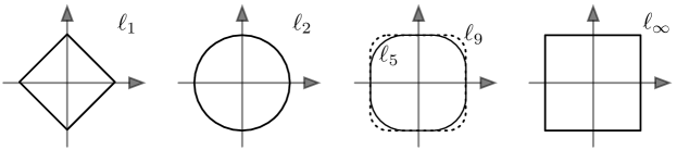
Figure 1: The unit disks $\{v\in{}^{2}\,|\,\|v\|{}=1\}$ in the $\ell_{1}$, $\ell_{2}$, $\ell_{p}$ for $p\in\{5,9\}$, and $\ell_{\infty}$ norms.

Given a positive definite $P$ and a positive vector $\eta$, we also define $\|x\|_{2,P}=(x^{\top}Px)^{1/2}$ and $\|x\|_{\infty,\eta}=\max_{i}|x_{i}|/\eta_{i}$. Given $A\in{}^{n\times n}$, a norm $\|\cdot\|$ on ⁿ induces a matrix norm and a matrix log norm defined by

$$\|A\|:=\max_{\|x\|=1}\|Ax\|\quad\text{and}\quad\mu(A):=\lim_{h\to 0^{+}}\frac{\|I_{n}+hA\|-1}{h}.$$

Closed form expressions are known for matrix norms and matrix log norms for all norms defined above, e.g., see [12, Chapter 2]. Matrix norms and matrix log norms enjoy a wide range of properties, including subadditivity, positive scaling, convexity, as well as certain monotonicity properties. Figure 2 illustrates how they are related to the eigenvalues of $A$.

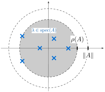
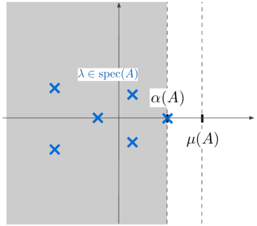
Figure 2: Given $A\in{}^{n\times n}$ with spectrum $\operatorname{spec}(A)$, the induced norm $\|A\|$ is an upper bound on the spectral radius $\rho(A)$ (left panel) and the induced log norm $\mu(A)$ is an upper bound on the spectral abscissa $\alpha(A)$ (right panel).

Discrete-time contractivity via Lipschitz constants

We consider discrete-time dynamical systems and their contractivity via Lipschitz constants. We consider

$$x_{k+1}=\mathsf{F}(x_{k}) \|\cdot\|{} \|\cdot\|{}$$ on ⁿ with norm and induced norm

The Lipschitz constant of $\mathsf{F}$ is equivalently defined by

$$\operatorname{\mathsf{Lip}}(\mathsf{F}) =\inf\{\ell>0\,\,|\,\,\|\mathsf{F}(x)-\mathsf{F}(y)\|{}\leq\ell\|x-y\|{}\text{ for all }x,y\}$$

$$=\sup\nolimits_{x}\|D\mkern-1.0mu{\mathsf{F}}(x)\|{}$$

For a scalar map $f\colon\real\rightarrow\real$, we have $\operatorname{\mathsf{Lip}}(f)=\sup_{x}|f(x)|$. Given a scalar $\ell$ and an affine map $\mathsf{F}_{A}(x)=Ax+a$, for $A\in{}^{n\times{n}}$ and $a\in{}^{n}$, we note the equivalences:

$$\operatorname{\mathsf{Lip}}_{2,P}(\mathsf{F}_{A})=\|A\|_{2,P}\leq\ell\qquad \iff\qquad A^{\top}PA\preceq\ell^{2}P$$

$$\operatorname{\mathsf{Lip}}_{\infty,\eta}(\mathsf{F}_{A})=\|A\|_{\infty,\eta}\leq\ell\qquad \iff\qquad\eta^{\top}|A|\leq\ell\eta^{\top}$$

Loosely-speaking, the computation of the Lipschitz constant of an affine map is equivalent to a semidefinite feasibility program in the weighted $\ell_{2}$ case and a linear program in the weighted $\ell_{\infty}$ case. With these concepts at hand, the Banach contraction theorem for discrete-time dynamics states that, if $\rho:=\operatorname{\mathsf{Lip}}(\mathsf{F})<1$, then

1. the map $\mathsf{F}$ is strongly contracting, i.e., the distance between any two trajectories decreases exponentially fast (with contraction factor $\rho$), and

2. $\mathsf{F}$ has a globally exponentially stable equilibrium $x^{*}$.

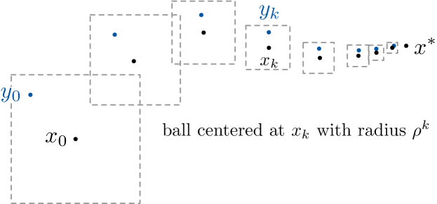
Figure 3: The Banach contraction theorem for discrete-time dynamics: Given initial conditions $x_{0}$, $y_{0}$ with $\|x_{0}-y_{0}\|\leq 1$, $y_{k}$ remains inside the ball centered at $x_{k}$ with radius $\rho^{k}$ and both trajectories converge exponentially fast to a limiting point $x^{*}$.

Log norm	differential	integral
condition	condition	condition
$\displaystyle\mu_{2,P}(D\mkern-1.0mu{\mathsf{F}}(x))\leq b$	$\displaystyle PD\mkern-1.0mu{\mathsf{F}}(x)+D\mkern-1.0mu{\mathsf{F}}(x)^{\top}P\preceq 2bP$	$\displaystyle(x-y)^{\top}P\big{(}\mathsf{F}(x)-\mathsf{F}(y)\big{)}\leq b\|x-y\|_{P^{1/2}}^{2}$
$\displaystyle\mu_{1}(D\mkern-1.0mu{\mathsf{F}}(x))\leq b$	$\displaystyle\operatorname{sign}(v)^{\top}D\mkern-1.0mu{\mathsf{F}}(x)v\leq b\|v\|_{1}$	$\displaystyle\operatorname{sign}(x-y)^{\top}(\mathsf{F}(x)-\mathsf{F}(y))\leq b\|x-y\|_{1}$
$\displaystyle\mu_{\infty}(D\mkern-1.0mu{\mathsf{F}}(x))\leq b$	$\displaystyle\max_{i\in I_{\infty}(v)}\!v_{i}\left(D\mkern-1.0mu{\mathsf{F}}(x)v\right)_{i}\leq b\|v\|_{\infty}^{2}$	$\displaystyle\max_{i\in I_{\infty}(x-y)}\!(x_{i}-y_{i})(\mathsf{F}_{i}(x)-\mathsf{F}_{i}(y))\leq b\|x-y\|_{\infty}^{2}$

Table 1: Table of equivalent contractivity conditions for a vector field $\mathsf{F}\colon{}^{n}\rightarrow{}^{n}$ from [28]. Each row contains three equivalent statements for the weighted $\ell_{2}$, $\ell_{1}$, and $\ell_{\infty}$ norm, respectively. Each statement is to be understood for all $x,y\in{}^{n}$ and all $v\in{}^{n}$. Equation (1) corresponds to the first column. The second column contains generalized version of the classic Demidovic condition for the existence of a common Lyapunov function. The third column contains “integral” conditions that do not require differentiability of $\mathsf{F}$. The function $\operatorname{sign}\colon{}^{n}\rightarrow\{-1,0,1\}^{n}$ is the entrywise $\operatorname{sign}$ function. We adopt the shorthand $I_{\infty}(v)=\{i\in\{1,\dots,n\}\,|\,|v_{i}|=\|v\|_{\infty}\}$.

Continuous-time contractivity via one-sided Lipschitz constants

Next we present a perfectly parallel treatment of the continuous-time case. We consider continuous-time dynamical systems and their contractivity via one-sided Lipschitz constants. We consider

$$\dot{x}=\mathsf{F}(x) \|\cdot\|{} \mu(\cdot)$$ on ⁿ with norm and induced log norm

The one-sided Lipschitz constant of $\mathsf{F}$ is defined by

$$\operatorname{\mathsf{osL}}(\mathsf{F}) =\sup\nolimits_{x}\mu(D\mkern-1.0mu{\mathsf{F}}(x))$$ (1)

and we refer to Table 1 for more general and equivalent definitions. For a scalar map $f\colon\real\rightarrow\real$, we have $\operatorname{\mathsf{osL}}(f)=\sup_{x}f^{\prime}(x)$. Given a scalar $\ell$ and an affine map $\mathsf{F}_{A}(x)=Ax+a$, for $A\in{}^{n\times{n}}$ and $a\in{}^{n}$, we note the equivalences:

$$\operatorname{\mathsf{osL}}_{2,P}(\mathsf{F}_{A})=\mu_{2,P}(A)\leq\ell\enspace \iff\enspace A^{\top}P+AP\preceq 2\ell P$$

$$\operatorname{\mathsf{osL}}_{\infty,\eta}(\mathsf{F}_{A})=\mu_{\infty,\eta}(A)\leq\ell\enspace \iff\enspace a_{ii}+\sum_{j\neq i}|a_{ij}|\eta_{i}/\eta_{j}\leq\ell$$

Again, the computation of the one-sided Lipschitz constant of an affine map is equivalent to a semidefinite feasibility program in the weighted $\ell_{2}$ case and a linear program in the weighted $\ell_{\infty}$ case. With these concepts at hand, the Banach contraction theorem for continuous-time dynamics states that, if $-c:=\operatorname{\mathsf{osL}}(\mathsf{F})<0$, then

1. the vector field $\mathsf{F}$ is strongly infinitesimally contracting, i.e., the distance between any two trajectories decreases exponentially fast (with contraction rate $c$), and

2. $\mathsf{F}$ has a globally exponentially stable equilibrium $x^{*}$.

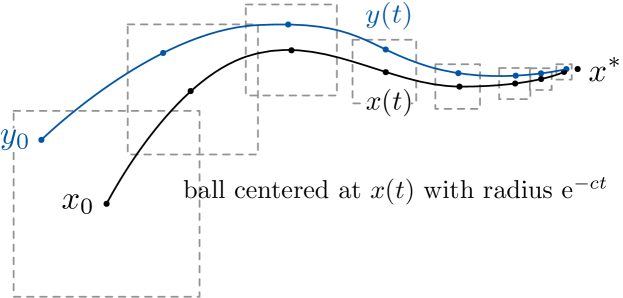
Figure 4: The Banach contraction theorem for continuous-time dynamics: Given initial conditions $x_{0}$, $y_{0}$ with $\|x_{0}-y_{0}\|\leq 1$, $y(t)$ remains inside the ball centered at $x(t)$ with radius $\mathrm{e}^{-ct}$ and both trajectories converge exponentially fast to a limiting point $x^{*}$.

Table of contractivity conditions

As promised at the beginning of this section, we are finally ready to provide a unifying table of contractivity conditions emerging from classical and modern works. Table 1, taken from [28], see also [3], provides three equivalent continuous-time contractivity conditions (namely, log norm, integral and differential conditions) for the $\ell_{2}$, $\ell_{1}$ and $\ell_{\infty}$ norms. The table summarizes the following classical and modern works:

• $\ell_{2}$ log norm condition (each row, first entry): classic work [34];

• $\ell_{2}$ differential condition (first row, second entry): classic work [33, 59] and its Riemannian generalization [61];

• $\ell_{2}$ integral condition (first row, third entry): see the discussion in the Introduction;

• $\ell_{1}$ integral condition (second row, third entry): due to work on neural networks and traffic networks [72, 19]; and

• $\ell_{\infty}$ conditions (third row): second and third entry are only very recently discovered [28].

2 Contractivity is robust, computationally-friendly, and modular stability

We now present some selected properties enjoyed by strongly contracting dynamical systems. We mostly focus on the continuous-time case, but equivalent properties hold also in discrete time. To illustrate our Opinion #2, we present robustness, computational, and modularity properties.

We start with a well-known robustness property [61] with respect to input disturbances and a recent extension [27] to the tracking of equilibrium trajectories.

Property 1 (Incremental input-to-state stability (iISS) and equilibrium tracking):

Consider a dynamical system subject to an input $\dot{x}=\mathsf{F}(x,\theta(t))$. Assume

• (contractivity with respect to $x$:) $\displaystyle\operatorname{\mathsf{osL}}_{x}(\mathsf{F})\leq-c<0$, uniformly in $\theta$, and

• (Lipschitz with respect to $\theta$:) $\displaystyle\operatorname{\mathsf{Lip}}_{\theta}(\mathsf{F})\leq\ell$, uniformly in $x$.

Then the system enjoys the incrementally ISS property (see Figure 6), namely for any two trajectories $x(t)$ and $y(t)$,

$$\|x(t)-y(t)\|\leq\mathrm{e}^{-ct}\|x_{0}-y_{0}\|\\ +\frac{\ell}{c}(1-\mathrm{e}^{-ct})\sup_{\tau\in[0,t]}\|\theta_{x}(\tau)-\theta_{y}(\tau)\|{}.$$

Additionally, at fixed $\theta$, let $x^{*}(\theta)$ be the unique of equilibrium of $\dot{x}=\mathsf{F}(x,\theta)$. Then the system enjoys the equilibrium tracking property (see Figure 6), namely

$$\|x(t){-}x^{*}(\theta(t))\|\leq\mathrm{e}^{-ct}\|x_{0}{-}x^{*}(\theta_{0})\|\\ +\frac{\ell}{c^{2}}(1-\mathrm{e}^{-ct})\sup_{\tau\in[0,t]}\|\dot{\theta}(\tau)\|$$

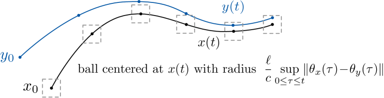
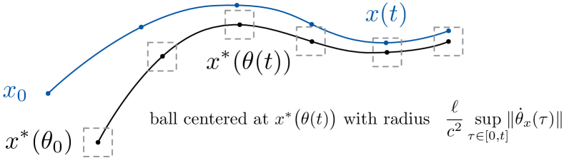
Figure 5: The incremental ISS property: each two trajectories $x(t)$ and $y(t)$ determined by inputs $\theta_{x}(t)$ and $\theta_{y}(t)$ respectively, asymptotically reach a distance upper bounded by $\frac{\ell}{c}\sup_{\tau}\|\theta_{x}(\tau)-\theta_{y}(\tau)\|{}$.

Figure 6: The equilibrium tracking property: each trajectory $x(t)$ asymptotically reaches a distance from the equilibrium trajectory $x^{*}\bigl{(}\theta(t)\bigr{)}$ upper bounded by $\frac{\ell}{c^{2}}\sup_{\tau}\|\dot{\theta}(\tau)\|{}$.

Next, we present a computational result explaining a close relationship between continuous and discrete-time contracting systems.

Property 2 (Euler discretization):

Given arbitrary norm $\|\cdot\|{}$ and Lipschitz $\mathsf{F}\colon{}^{n}\rightarrow{}^{n}$, the following statements are equivalent:

1. $\dot{x}=\mathsf{F}(x)$ is strongly infinitesimally contracting, and

2. there exists $\alpha>0$ such that $x_{k+1}=x_{k}+\alpha\mathsf{F}(x_{k})$ is strongly contracting.

Guidelines for the selection of an optimal step-size are available: the optimal choice depends upon the norm. We refer to [13] for guidance on step-size selection. Finally, we present a result about the modularity properties of contracting systems.

Property 3 (Network contractivity):

Consider $n$ interconnected subsystems described by

$$\dot{x}_{i}=\mathsf{F}_{i}(x_{i},x_{-i}),\qquad\text{for }i\in\{1,\dots,n\}$$

where $x_{i}\in{}^{N_{i}}$ is the state of the $i$th subsystem and $x_{-i}\in{}^{N-N_{i}}$ are the states of all other subsystems. Assume that

• (contractivity with respect to $x_{i}$:) $\displaystyle\operatorname{\mathsf{osL}}_{x_{i}}(\mathsf{F}_{i})\leq-c_{i}<0$, uniformly in $x_{-i}$

• (Lipschitz with respect to $x_{j}$, $j\neq{i}$:) $\displaystyle\operatorname{\mathsf{Lip}}_{x_{j}}(\mathsf{F}_{i})\leq\ell_{ij}$, uniformly in $x_{-j}$, and

• the gain matrix $\Gamma=\begin{bmatrix}-c_{1}&\dots&\ell_{1n}\\ \vdots&&\vdots\\ \ell_{n1}&\dots&-c_{n}\end{bmatrix}$ is Hurwitz.

Then the interconnected system is strongly infinitesimally contracting with rate equal to $|\alpha(\Gamma)|$.

Note that the Hurwitz assumption on the Metzler matrix $\Gamma$ is equivalent to a small gain theorem [38] and that there are other interconnection theorem based upon times scale separation [31, 22].

3 Numerous dynamical systems are contracting

The simplest example or a discrete-time (resp., continuous-time) contracting dynamics is the case of a linear system with a Schur (resp, Hurwitz) matrix. This is due to the existence of efficient norms, see [12, Chapter 2]. This observation can be easily extended to feedback linearizable systems with stabilizing controllers. We now present three important examples of continuous-time contracting dynamics from convex optimization, neural networks, and nonlinear control.

Gradient descent in optimization

Given a function $f\colon{}^{n}\rightarrow\real$, the following are equivalent statements:

1. $f$ is strongly convex with parameter $\nu$ (and global minimum $x^{*}\in{}^{n}$), and

2. the gradient descent vector field $\mathsf{F}_{\textup{grad}}:=-\nabla{f}$ is strongly infinitesimally contracting with respect to $\|\cdot\|_{2}$ with rate $\mu$ (and equilibrium $x^{*}$).

This result is also known as Kachurovskii’s Theorem [53]. Many other related dynamical systems are contracting [47] under strong convexity assumptions, including primal-dual gradient descent, incidence- and Laplacian-based distributed gradient descent, proximal gradient descent as well as saddle dynamics, pseudo-gradient descent and best response play from game theory.

Firing rate models in recurrent neural networks

Next, we consider the firing rate model for recurrent neural networks

$$\dot{x}=-Cx+\Phi(Ax+u)=:\mathsf{F}_{\textup{FR}}(x).$$ (2)

where the dissipation matrix $C\in{}^{n\times n}$ is diagonal and positive semi-definite, the synaptic matrix $A\in{}^{n\times n}$ is invertible, $u\in{}^{n}$ is a constant bias, and $\Phi\colon{}^{n}\rightarrow{}^{n}$ is an activation function for the form $\Phi(x)=(\phi_{1}(x_{1}),\dots,\phi_{n}(x_{n}))$, where each $\phi_{i}\colon\real\rightarrow\real$ satisfies

$$d_{\textup{1}} :=\inf_{x,y\in\real,x\neq y}\frac{\phi_{i}(x)-\phi_{i}(y)}{x-y},$$ (3)

$$d_{\textup{2}} :=\sup_{x,y\in\real,x\neq y}\frac{\phi_{i}(x)-\phi_{i}(y)}{x-y}.$$

for appropriate finite $d_{\textup{1}}\leq d_{\textup{2}}$, see the examples in Figure 7. Then

$$\operatorname{\mathsf{osL}}_{\infty}(\mathsf{F}_{\textup{FR}})=\max\{\mu_{\infty}(-C+d_{\textup{1}}A),\mu_{\infty}(-C+d_{\textup{2}}A)\},$$

In other words, when $d_{\textup{1}}=0$, $d_{\textup{2}}=1$, $C=I_{n}$, and $\operatorname{relu}\bigl{(}\mu_{\infty}(A)\bigr{)}<1$, we know

$$\operatorname{\mathsf{osL}}_{\infty}(\mathsf{F}_{\textup{FR}})=-1+\operatorname{relu}\bigl{(}\mu_{\infty}(A)\bigr{)}$$

so that the firing rate model (2) is strongly infinitesimally contracting with respect to $\|\cdot\|_{\infty}$ with rate $1-\operatorname{relu}\bigl{(}\mu_{\infty}(A)\bigr{)}$.

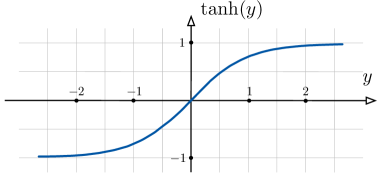
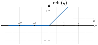
Figure 7: Hyperbolic tangent and relu functions satisfy the constraint $d_{\textup{1}}=0\leq\phi_{i}^{\prime}(y)\leq 1=d_{\textup{2}}$ almost everywhere.

This result follows from maximizing a convex function on a polytope. We refer to [29] for a comprehensive sharp treatment of contractivity of continuous-time recurrent neural networks with respect to optimally-weighted non-Euclidean norms.

Lur’e models in nonlinear control

Given matrices $A\in{}^{n\times{n}}$, $B\in{}^{n\times{m}}$, $C\in{}^{m\times{n}}$ and a map $\varphi\colon{}^{m}\rightarrow{}^{m}$, consider the Lur’e system

$$\dot{x}=Ax+B\varphi(Cx):=\mathsf{F}_{\textup{Lur'e}}(x).$$ (4)

We consider maps $\varphi$ for which $\rho>0$ exists such that

$$(\varphi(y_{1})-\varphi(y_{2}))^{\top}(y_{1}-y_{2})\geq\rho\|\varphi(y_{1})-\varphi(y_{2})\|_{2}^{2}$$ (5)

for all $y_{1},y_{2}\in{}^{m}$ (such maps are referred to as cocoercive). Given a positive definite $P\in{}^{n\times n}$ and $\eta>0$, the following statements are equivalent:

1. the Lur’e system (4) is strongly infinitesimally contracting with respect to $\|\cdot\|_{2,P}$ with rate $\eta$ for any $\varphi$ satisfying (5),

2. there exists $\lambda\geq 0$ such that

   $$\begin{bmatrix}A^{\top}P+PA+2\eta P&PB+\lambda C^{\top}\\ B^{\top}P+\lambda C&-2\lambda\rho I_{m}\end{bmatrix}\preceq 0.$$ (6)

In other words, the LMI (6) is necessary and sufficient for

$$\sup_{\varphi\text{ satisfying }\eqref{eq:monotonicity}}\operatorname{\mathsf{osL}}(\mathsf{F}_{\textup{Lur'e}})=-\eta.$$

This result follows from a careful application of the S-lemma.

4 Contraction theory is relevant to modern applications

We here briefly review three application areas.

Optimization-based control

We argue that contraction theory is relevant in a wide range of optimization and optimization-based control problems, e.g., including parametric optimization, model predictive control [54], control barrier functions, and online feedback optimization, as we show below. We focus on continuous-time systems here for simplicity of notation.

Since many convex optimization problems can be solved with contracting dynamics (meaning that the minimizer of the optimization problem is the equilibrium point of the dynamics):

$$\min\mathcal{E}(x)\quad\iff\quad\dot{x}=\mathsf{F}(x),$$

it is possible to use contraction theory to analyze parametric and time-varying convex optimization, or, more precisely, parametric and time-varying contracting dynamics:

$$\min\mathcal{E}(x,\theta)\quad \iff\quad\dot{x}=\mathsf{F}(x,\theta)$$

$$\min\mathcal{E}\bigl{(}x,\theta(t)\bigr{)}\quad \iff\quad\dot{x}=\mathsf{F}\bigl{(}x,\theta(t)\bigr{)}$$

where $\theta$ is either constant of time-varying.

Recent optimization-based control efforts [18, 49] have focused on online feedback optimization. In this approach, they key idea is to regulate the input-output pair $(u,y)$ of a dynamical system subject to a disturbance $w(t)$.

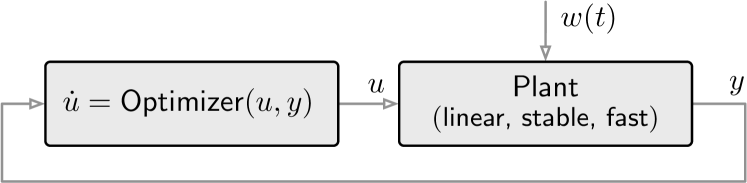
Figure 8: Online feedback optimization: typical setup and assumptions

As illustrated in Figure 8, we aim to find the optimal control $u$ minimizing:

$$\begin{cases}\min\quad&\text{cost}_{1}(u)+\text{cost}_{2}(y)\\ \text{subj. to}\quad&y=\mathsf{Plant}\big{(}u,w(t)\big{)}\end{cases}$$

Specifically, assuming a linear relationship from input $u$ and disturbance $w$ to the output $y$, we define

$$u^{*}\bigl{(}w(t)\bigr{)}:=\;\operatorname*{arg\,min}_{u}\;\; \;\phi(u)+\psi(y(t))$$

subj to $$\;y(t)=Y_{u}u+Y_{w}w(t)$$

where we design $\phi$ to be strongly convex with parameter $\mu$ and $\psi$ to be convex. Instead of exactly computing $u^{*}\bigl{(}w(t)\bigr{)}$ at each instant of time, we define the gradient controller

$$\dot{u}=\mathsf{F}_{\textup{GradCtrl}}(u,w)\\ \;:=\;-\nabla_{u}\mathcal{E}(u,w)=-\nabla\phi(u)-Y_{u}^{\top}\nabla\psi(Y_{u}u+Y_{w}w)$$

Since the gradient descent of a strongly convex function is strongly contracting (see Section 3), Property 1 implies that the gradient controller tracks the optimal controller satisfying:

$$\limsup_{t\to\infty}\|u(t)-u^{*}\bigl{(}w(t)\bigr{)}\|\quad\leq\quad\frac{\ell_{w}}{\nu^{2}}\;\limsup_{t\to\infty}\|\dot{w}(t)\|$$

where

1. $\operatorname{\mathsf{osL}}_{u}(\mathsf{F}_{\textup{GradCtrl}})\leq-\nu$, and

2. $\operatorname{\mathsf{Lip}}_{w}(\mathsf{F}_{\textup{GradCtrl}})=\ell_{w}:=\|Y_{u}^{\top}\|{}\operatorname{\mathsf{Lip}}(\nabla\psi)\|Y_{w}\|{}$

We refer to [22] for a more complete contractivity analysis based upon singular perturbation methods.

Implicit and reservoir models in machine learning

A second broad application area for contraction theory is the design of machine learning models. The idea is to use contractivity properties to establish accurate, reproducible, and robust behavior in face of uncertain stimuli and dynamics.

We here briefly review two models. First, implicit neural networks (NNs) [40, 52], also called deep equilibrium networks [6], are a class of implicit-depth learning models that generalize feedforward neural network models and have demonstrated improved accuracy and reduction in memory requirements, see Figure 9.

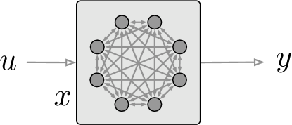
Figure 9: Implicit NNs embed feedback loops in their input-output relationship, unlike feedforward machine learning models. In these models function evaluation is performed by solving a fixed point equation.

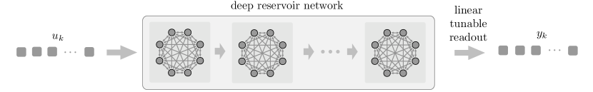
Figure 10: An example deep architecture for a reservoir computer [44]. Based upon our discussion, this deep reservoir network is contracting if each reservoir’s synaptic matrix satisfies the log norm condition $\mu_{\infty}(A^{(i)})<1$.

As starting point we consider the fixed point equation

$$x =\Phi(Ax+Bu+b)$$ (7)

whose solution is the equilibrium of both a continuous-time firing rate model and its Euler discretization (also called leaky integrator neurons):

$$\dot{x} =-x+\Phi(Ax+Bu+b)$$ (8)

$$x_{k+1} =(1-\alpha)x_{k}+\alpha\Phi(Ax_{k}+Bu+b)$$ (9)

In light of the previous sections and [52], if the synaptic matrix is designed to satisfy $\mu_{\infty}(A)<1$, then (adopting the shorthand $(v)_{+}:=\operatorname{relu}(v),(v)_{-}:=-\operatorname{relu}(-v)$)

• the implicit NN (7) has a unique solution $x^{*}(u)$,

• the continuous-time model (8) is infinitesimally contracting with rate $1-(\mu_{\infty}(A))_{+}$,

• the discrete-time model (9) is contracting with factor $\displaystyle 1-\frac{1-(\mu_{\infty}(A))_{+}}{1-\min_{i}(a_{ii})_{-}}$ at the optimal step size $\alpha^{*}=\frac{1}{1-\min_{i}(a_{ii})_{-}}$.

Additionally, the model (7) is robust in the sense that

$$\operatorname{\mathsf{Lip}}_{u\to x}=\frac{\|B\|_{\infty}}{1-(\mu_{\infty}(A))_{+}},\;\text{and}\;\frac{\|\Delta x^{*}\|_{\infty}}{\|x^{*}\|_{\infty}}\leq\frac{\|\Delta A\|_{\infty}}{1-(\mu_{\infty}(A))_{+}}.$$

As second machine learning application we briefly mention reservoir computing, illustrated in Figure 10. This class of machine learning models was introduced in [50, 64] to process temporal and sequential data. In these models, a critical property is that the reservoir state asymptotically depends only on the input stimulus, while the influence of initial conditions should asymptotically vanish. This property is called the echo state property (namely, the state should be an echo of the input, not of the initial conditions) or the fading memory property — and it is an immediate consequence of contractivity. Obtaining sharp contractivity estimates is crucial since reservoir computers appear to work best when at the edge of stability.

Biologically-plausible competitive neural networks

Finally, we briefly present an application to biologically-plausible neural circuits. Understanding the functionality of recurrent neural networks is a major neuroscientific objective; we refer to [68] for a review of neuroscience-inspired learning and signal processing algorithms.

An important problem in this context is the study of neural networks capable of solving dimensionality-reduction problems and, specifically, sparse reconstruction problems. These problems involve approximating a given input stimulus with a set of sparse active neurons. Here is a simplified problem setup from [74, 16]. Given an input stimulus $u\in{}^{M}$, a vector of neural activations $x\in{}^{N}$, and a scalar $\lambda$, the neural circuit aims to solve

$$\min_{x\in{}^{N},x\geq 0}\quad\underbrace{\tfrac{1}{2}\|u-\Phi x\|_{2}^{2}}_{\text{reconstruction error}}\quad+\quad\underbrace{\lambda\;\|x\|_{1}}_{\text{sparsity-promoting regularizer}}$$ (10)

Here $\Phi\in{}^{M\times{N}}$ is a highly redundant ($N\gg M$) nonnegative dictionary matrix with unit-norm columns ($\|\Phi_{i}\|{}=1$). Using concepts from proximal operators and contraction theory one can design and confirm the functionality of the positive firing-rate competitive network (see Figure 11):

$$\dot{x}_{i}(t)=-x_{i}+\operatorname{relu}\bigl{(}-\sum\nolimits_{j=1,j\neq{i}}^{n}\Phi_{i}^{\top}\Phi_{j}x_{j}+\Phi_{i}^{\top}u-\lambda\bigr{)}.$$ (11)

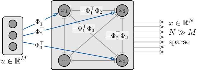
Figure 11: Diagram illustrating the positive competitive neural network (11). The competition between each two neurons $i$ and $j$ is proportional to $\Phi_{i}\cdot\Phi_{j}$, the similarity between columns $i$ and $j$.

Specifically, equilibrium points of (11) are minimizers of (10) and if $x_{i}(0)\geq 0$, then $x_{i}(t)\geq 0$ for all $t\geq 0$. Moreover, under a restricted isometry property of the dictionary matrix, the dynamics are locally contracting [16].

        

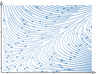
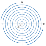
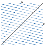
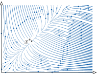
Figure 12: The dichotomy property for weakly-contracting systems: either each trajectory is unbounded or each trajectory is bounded. Left panel: every trajectory is unbounded and the system has no equilibrium. Right panel (with three images): every trajectory is bounded, the system has at either one or infinitely many equilibria and local asymptotic stability of an equilibrium implies global asymptotic stability.

5 Contraction theory can be vastly extended in numerous directions

While contracting dynamical systems enjoy numerous desirable properties, there are many systems that are not contracting yet enjoy similar properties. To this end, many variations on contraction theory have been proposed and in this section, we highlight three extensions to the original theory.

5.1 Weakly Contracting Dynamics

Systems with conserved quantities or translational invariance cannot possibly be contracting since the system trajectories cannot fully forget initial conditions. For example, continuous-time flow networks and continuous-time averaging are examples of linear systems which obey this conservation and invariance property, respectively. However, both of these dynamics (and many others) enjoy a different property, known as weak infinitesimal contraction (or infinitesimal nonexpansiveness), where the distance between trajectories is nonincreasing. Stated more concretely, a dynamical system $\dot{x}=\mathsf{F}(x)$, is weakly infinitesimally contracting if $\mu(D\mkern-1.0mu{\mathsf{F}}(x))\leq 0$ for all $x$. In analogy to standard nonexpansive maps, weakly infinitesimally contracting dynamics induce flows which are nonexpansive for all $t\geq 0$.

In line with the theory of nonexpansive maps, weakly contracting dynamical systems obey a dichotomy property. Either every trajectory is unbounded (i.e., no equilibrium point exists) or every trajectory is bounded and there exists at least one equilibrium point [51]. Moreover, if there exists an equilibrium point which is locally asymptotically stable, then it is also globally asymptotically stable. See Figure 12 for examples of weakly contracting dynamical systems.

5.2 Locally Contracting Dynamics

Although it is desirable to ensure global contraction, in many practical examples, dynamics are only contracting in a region (possibly, but not necessarily, containing an equilibrium point). For example, gradient descent for nonconvex objective functions is locally contracting in a neighborhood of a local minimizer if and only if the objective function is strongly convex in the same neighborhood.

In short, if there exists a convex forward-invariant set, $\mathcal{C}$, for the dynamical system, $\dot{x}=\mathsf{F}(x)$, then all the standard consequences of contractivity hold for all trajectories remaining inside the set, e.g., the existence of a unique equilibrium point $x^{*}\in\mathcal{C}$. The challenge is thus in finding a set, $\mathcal{X}$, for which $\mu(D\mkern-1.0mu{\mathsf{F}}(x))\leq-c$ for all $x\in\mathcal{X}$ and then finding a forward invariant set, $\mathcal{C}\subseteq\mathcal{X}$. In Figure 13, we plot an instance of a locally contracting system.

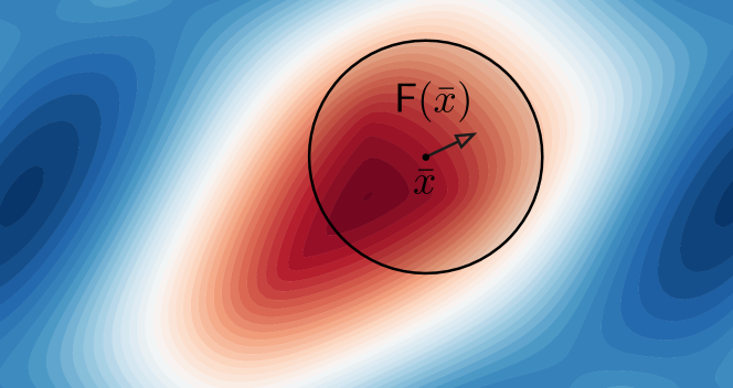
Figure 13: Illustration of a locally contracting vector field. Given a vector field $\mathsf{F}$ on a planar domain and a norm, the contour plot shows values of the quantity $\mu(D\mkern-1.0mu{\mathsf{F}})$: red values correspond to regions where the vector field $\mathsf{F}$ is strongly infinitesimally contracting $\mu(D\mkern-1.0mu{\mathsf{F}}(x))<0$ and blue values correspond to regions where $\mu(D\mkern-1.0mu{\mathsf{F}}(x))>0$. To establish the existence of a forward-invariant set, it is useful to find a closed ball centered at $\overline{x}$ inside the red region, with small residual $\|\mathsf{F}(\overline{x})\|{}$.

5.3 Contraction Theory on Manifolds

Contraction theory on Riemannian manifolds was initiated by the seminal work [61]. In brief summary, given a system $\dot{x}=\mathsf{F}(x)$ with $x\in{}^{n}$, it is proposed to give ⁿ the structure of a Riemannian manifold by introducing a mapping $M\colon{}^{n}\rightarrow{}^{n\times n}$ and two positive constants $a_{0},a_{1}>0$ satisfying $M(x)=M(x)^{\top}$ and $a_{0}I_{n}\preceq M(x)\preceq a_{1}I_{n}$ for all $x\in{}^{n}$. Then, $M(x)$ induces a state-dependent norm on ⁿ, $\|\cdot\|_{M(x)}$ or, more precisely, a state-dependent inner product $\left\langle\!\left\langle{\cdot},{\cdot}\right\rangle\!\right\rangle_{M}$ and Riemannian metric. The dynamical system is contracting with respect to this Riemannian metric with rate $c>0$ if

$$M(x)D\mkern-1.0mu{\mathsf{F}}(x)+D\mkern-1.0mu{\mathsf{F}}(x)^{\top}M(x)+\dot{M}(x)\preceq-2cM(x),$$ (12)

for all $x\in{}^{n}$. Here, the quantity $\dot{M}$ is a shorthand for the Lie derivative of $M$ along trajectories of $\dot{x}=\mathsf{F}(x)$. The state-dependent LMI (12) is a generalization of the classical result by Demidovich. In the context of log norms, if $M(x)=\Theta(x)^{\top}\Theta(x)$, the LMI (12) is equivalent to asking that

$$\mu_{2}\bigl{(}\Theta(x)D\mkern-1.0mu{\mathsf{F}}(x)\Theta(x)^{-1}+\dot{\Theta}(x)\Theta(x)^{-1}\bigr{)}\leq-c.$$

In short, contraction with respect to a Riemannian metric ensures that the geodesic distance between any two trajectories is exponentially decaying. See Figure 14 for an illustrative example of contraction on a Riemannian manifold.

Since the seminal work by Lohmiller and Slotine, much interest has focused on contraction theory on manifolds. In [78], a formal coordinate-free analysis was provided. In [42], the theory was extended to Finsler manifolds. Finally, in [66], the theory was extended to design controllers such that the closed-loop system is guaranteed to be contracting with respect to a certain Riemannian metric.

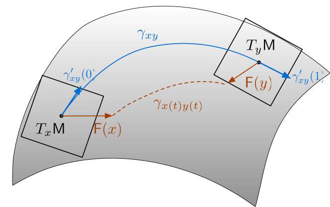
Figure 14: Contractivity of a vector field $\mathsf{F}$ on a Riemannian manifold: the length of the geodesic curve $\gamma_{xy}$ connecting any two points $x$ and $y$ decreases along the flow of $\mathsf{F}$, as a function of the inner product between $\mathsf{F}$ and the geodesic velocity vector at $x$ and $y$.

6 Conjectures and Future Directions

We conclude this opinion paper with some open problems in theory, applications, and computation.

Theory

While the theoretical underpinnings of contraction theory with respect to norms and Riemannian metrics are largely understood, there remain many fundamental open problems surrounding sharpness of contraction conditions and their extensions. For example, sharp characterizations of contractivity exist for some special dynamical systems (e.g., gradient flow, firing rate neural networks, and certain Lur’e models), yet there are other relatively simple dynamical systems whose sharpest rates of contraction are still unknown, e.g., primal dual dynamics for linear equality-constrained minimization and Hopfield neural networks with diagonally stable synaptic matrices.

At the same time, a comprehensive understanding of the recent theoretical extensions of $p$-dominance [43, 77], $k$- and $\alpha$-contraction [84, 83, 8] is still missing along with rich sets of examples and necessary and sufficient conditions for establishing these properties.

Additionally, an input-output perspective on contracting systems appears largely missing. Namely, comparisons between contracting systems and incrementally passive or dissipative systems could yield novel insights. In a similar vein, since contracting systems have properties akin to those of stable linear systems (apart from the superposition principle), it is natural to ask whether contracting systems admit frequency-domain analysis tools (see the early work [67] for ideas in this direction).

A final theoretical topic of interest is developing novel mathematical tools to establish contractivity. For contraction with respect to Euclidean norms, a useful tool is the S-Lemma [70] which provides conditions under which one quadratic inequality (e.g., contractivity) is implied by other quadratic inequalities (e.g., slope constraints on nonlinearities). For contraction with respect to non-Euclidean norms, a non-Euclidean S-Lemma was recently proposed in [71] and necessary and sufficient conditions for zero duality gap were shown in the case of the $\ell_{1}$ norm with Metzler matrices. It remains an open problem whether such results can be extended to other important cases such as contractivity with respect to the $\ell_{\infty}$ norm. Developments in this direction may rely upon the theory of integral linear constraints [11].

Applications

In Section 4, we presented three modern applications where contraction theory plays a pivotal role, namely optimization-based control, machine learning, and dynamical neuroscience. In each of these applications, there remains room for improvement. For example, contraction-theoretic tools are only recently coming to bear on the topics of suboptimal model predictive control and in control barrier functions. Specifically, the incremental input-to-state stability and equilibrium tracking properties may be used to provide novel robustness bounds to inaccurate solvers or uncertainty in the dynamics model.

Beyond these three applications, we list in the Introduction several other research areas where contractivity tools play an important role. For example, in the study of biochemical reaction networks, convergence and robustness properties are being established independently of specific forms of kinetics by leveraging contraction with respect to polyhedral norms [10, 1, 39]. Additionally, in the study of traffic networks, weak contraction with respect to the $\ell_{1}$ norm is adopted to establish the existence of steady state free-flow equilibria [19, 21].

In short, we believe that contraction theoretic ideas can be leveraged to analyze and design dynamical systems and algorithms in many disparate application domains.

Computation

In establishing contraction of a given dynamical system or closed-loop control system, the typical challenge is in finding with respect to what norm or Riemannian metric the system is contracting. Due to recent improvements in machine learning and numerical optimization solvers, several software packages have become available to either (i) numerically estimate contraction metrics, (ii) design controllers so that the closed-loop system is approximately contracting, or (iii) establish robustness guarantees of neural networks via a contraction analysis. For example, [86, 82] feature various versions of SOS-programming, gridding and interpolation, and neural network-based software for the computation of control contraction metrics. [9] provides a Julia package for neural networks and data-driven control with robustness guarantees ensured by contraction. Finally, [52] contains software to train implicit neural networks which are guaranteed to be contracting with respect to an $\ell_{\infty}$ norm.

Despite this progress, no single software library is comprehensive and widely accepted as the reference implementation in this area. An open challenge and burgeoning area of software engineering would be to create a robust codebase for establishing contractivity of structured nonlinear systems leveraging recent advances in nonlinear programming. An important extension to this codebase would be the ability to design controllers with guarantees of closed-loop contractivity.

Closing Thoughts

In this opinion paper, we have extolled the virtues of contraction theory and highlighted its universality and applicability. Specifically, we have argued that (i) contraction theory is a unifying framework emerging from classical and modern works, (ii) contractivity is a computationally-friendly, robust, and modular stability, (iii) numerous dynamical systems are contracting, (iv) contraction theory is relevant to modern applications, and (v) contraction theory can be vastly extended in numerous directions.

As a takeaway message for control theoreticians and engineers, we hope we have convinced them to:

(1) search for contraction properties,
(2) design engineering systems to be contracting, and
(3) verify correct and safe behavior via known
(4) Lipschitz and contractivity constants.

7 Acknowledgements

We would like to thank our coauthors and colleagues: Veronica Centorrino, Pedro Cisneros-Velarde, Sam Coogan, Lily Cothren, Emiliano Dall’Anese, Giulia De Pasquale, Robin Delabays, Xiaoming Duan, Anand Gokhale, Saber Jafarpour, Michael Margaliot, Ron Ofir, Anton Proskurnikov, Giovanni Russo, Francesco Seccamonte, John Simpson-Porco, Kevin Smith, and Maria Elena Valcher for all of their stimulating conversations.

References

- [1] M. A. Al-Radhawi, D. Angeli, and E. D. Sontag. On structural contraction of biological interaction networks. arXiv preprint arXiv:2307.13678, 2023.
- [2] Z. Aminzare. Stochastic logarithmic Lipschitz constants: A tool to analyze contractivity of stochastic differential equations. IEEE Control Systems Letters, 6:2311–2316, 2022. doi:10.1109/LCSYS.2022.3148945.
- [3] Z. Aminzare and E. D. Sontag. Contraction methods for nonlinear systems: A brief introduction and some open problems. In IEEE Conf. on Decision and Control, pages 3835–3847, December 2014. doi:10.1109/CDC.2014.7039986.
- [4] Z. Aminzare and E. D. Sontag. Synchronization of diffusively-connected nonlinear systems: Results based on contractions with respect to general norms. IEEE Transactions on Network Science and Engineering, 1(2):91–106, 2014. doi:10.1109/TNSE.2015.2395075.
- [5] V. Andrieu, B. Jayawardhana, and L. Praly. Transverse exponential stability and applications. IEEE Transactions on Automatic Control, 61(11):3396–3411, 2016. doi:10.1109/tac.2016.2528050.
- [6] S. Bai, J. Z. Kolter, and V. Koltun. Deep equilibrium models. In Advances in Neural Information Processing Systems, 2019. URL: https://arxiv.org/abs/1909.01377.
- [7] Stefan Banach. Sur les opérations dans les ensembles abstraits et leur application aux équations intégrales. Fundamenta Mathematicae, 3(1):133–181, 1922. doi:10.4064/fm-3-1-133-181.
- [8] E. Bar-Shalom, O. Dalin, and M. Margaliot. Compound matrices in systems and control theory: a tutorial. Mathematics of Control, Signals, and Systems, 35(3):467–521, 2023. doi:10.1007/s00498-023-00351-8.
- [9] N. J. Barbara, M. Revay, R. Wang, J. Cheng, and I. R. Manchester. RobustNeuralNetworks.jl: a package for machine learning and data-driven control with certified robustness, 2023. URL: http://arxiv.org/abs/2306.12612.
- [10] F. Blanchini and G. Giordano. Piecewise-linear Lyapunov functions for structural stability of biochemical networks. Automatica, 50(10):2482–2493, 2014. doi:10.1016/j.automatica.2014.08.012.
- [11] C. Briat. Robust stability and stabilization of uncertain linear positive systems via integral linear constraints: -gain and -gain characterization. International Journal of Robust and Nonlinear Control, 23(17):1932–1954, 2013. doi:10.1002/rnc.2859.
- [12] F. Bullo. Contraction Theory for Dynamical Systems. Kindle Direct Publishing, 1.1 edition, 2023, ISBN 979-8836646806. URL: https://fbullo.github.io/ctds.
- [13] F. Bullo, P. Cisneros-Velarde, A. Davydov, and S. Jafarpour. From contraction theory to fixed point algorithms on Riemannian and non-Euclidean spaces. In IEEE Conf. on Decision and Control, December 2021. doi:10.1109/CDC45484.2021.9682883.
- [14] T. Caraballo and P. E. Kloeden. The persistence of synchronization under environmental noise. Proceedings of the Royal Society A: Mathematical, Physical and Engineering Sciences, 461(2059):2257–2267, 2005. doi:10.1098/rspa.2005.1484.
- [15] V. Centorrino, F. Bullo, and G. Russo. Modelling and contractivity of neural-synaptic networks with Hebbian learning. Automatica, 164:111636, 2024. doi:10.1016/j.automatica.2024.111636.
- [16] V. Centorrino, A. Gokhale, A. Davydov, G. Russo, and F. Bullo. Positive competitive networks for sparse reconstruction. Neural Computation, January 2024. To appear. doi:10.48550/arXiv.2311.03821.
- [17] L. Chua and D. Green. A qualitative analysis of the behavior of dynamic nonlinear networks: Stability of autonomous networks. IEEE Transactions on Circuits and Systems, 23(6):355–379, 1976. doi:10.1109/TCS.1976.1084228.
- [18] M. Colombino, E. Dall’Anese, and A. Bernstein. Online optimization as a feedback controller: Stability and tracking. IEEE Transactions on Control of Network Systems, 7(1):422–432, 2020. doi:10.1109/TCNS.2019.2906916.
- [19] G. Como, E. Lovisari, and K. Savla. Throughput optimality and overload behavior of dynamical flow networks under monotone distributed routing. IEEE Transactions on Control of Network Systems, 2(1):57–67, 2015. doi:10.1109/TCNS.2014.2367361.
- [20] S. Coogan. A contractive approach to separable Lyapunov functions for monotone systems. Automatica, 106:349–357, 2019. doi:10.1016/j.automatica.2019.05.001.
- [21] S. Coogan and M. Arcak. A compartmental model for traffic networks and its dynamical behavior. IEEE Transactions on Automatic Control, 60(10):2698–2703, 2015. doi:10.1109/TAC.2015.2411916.
- [22] L. Cothren, F. Bullo, and E. Dall’Anese. Singular perturbation via contraction theory. IEEE Transactions on Automatic Control, October 2023. Submitted. doi:10.48550/arXiv.2310.07966.
- [23] G. Dahlquist. Stability and error bounds in the numerical integration of ordinary differential equations. PhD thesis, (Reprinted in Trans. Royal Inst. of Technology, No. 130, Stockholm, Sweden, 1959), 1958.
- [24] G. Dahlquist. Error analysis for a class of methods for stiff non-linear initial value problems. In G. A. Watson, editor, Numerical Analysis, pages 60–72. Springer, 1976. doi:10.1007/BFb0080115.
- [25] L. D’Alto and M. Corless. Incremental quadratic stability. Numerical Algebra, Control and Optimization, 3:175–201, 2013. doi:10.3934/naco.2013.3.175.
- [26] A. Davydov and F. Bullo. Exponential stability of parametric optimization-based controllers via Lur’e contractivity. IEEE Control Systems Letters, 2024. Submitted. doi:10.48550/arXiv.2403.08159.
- [27] A. Davydov, V. Centorrino, A. Gokhale, G. Russo, and F. Bullo. Contracting dynamics for time-varying convex optimization. IEEE Transactions on Automatic Control, June 2023. Submitted. doi:10.48550/arXiv.2305.15595.
- [28] A. Davydov, S. Jafarpour, and F. Bullo. Non-Euclidean contraction theory for robust nonlinear stability. IEEE Transactions on Automatic Control, 67(12):6667–6681, 2022. doi:10.1109/TAC.2022.3183966.
- [29] A. Davydov, A. V. Proskurnikov, and F. Bullo. Non-Euclidean contraction analysis of continuous-time neural networks. IEEE Transactions on Automatic Control, August 2023. Submitted. doi:10.48550/arXiv.2110.08298.
- [30] G. De Pasquale, K. D. Smith, F. Bullo, and M. E. Valcher. Dual seminorms, ergodic coefficients, and semicontraction theory. IEEE Transactions on Automatic Control, 69(5), 2024. To appear. doi:10.1109/TAC.2023.3302788.
- [31] D. Del Vecchio and J.-J. E. Slotine. A contraction theory approach to singularly perturbed systems. IEEE Transactions on Automatic Control, 58(3):752–757, 2013. doi:10.1109/TAC.2012.2211444.
- [32] P. DeLellis, M. Di Bernardo, and G. Russo. On QUAD, Lipschitz, and contracting vector fields for consensus and synchronization of networks. IEEE Transactions on Circuits and Systems I: Regular Papers, 58(3):576–583, 2011. doi:10.1109/TCSI.2010.2072270.
- [33] B. P. Demidovič. Dissipativity of a nonlinear system of differential equations. Uspekhi Matematicheskikh Nauk, 16(3(99)):216, 1961.
- [34] C. A. Desoer and H. Haneda. The measure of a matrix as a tool to analyze computer algorithms for circuit analysis. IEEE Transactions on Circuit Theory, 19(5):480–486, 1972. doi:10.1109/TCT.1972.1083507.
- [35] C. A. Desoer and M. Vidyasagar. Feedback Systems: Input-Output Properties. Academic Press, 1975, ISBN 978-0-12-212050-3. doi:10.1137/1.9780898719055.
- [36] M. Di Bernardo, D. Fiore, G. Russo, and F. Scafuti. Convergence, consensus and synchronization of complex networks via contraction theory. In Complex Systems and Networks, pages 313–339. Springer, 2016. doi:10.1007/978-3-662-47824-0_12.
- [37] S. S. Du, X. Zhai, B. Poczos, and A. Singh. Gradient descent provably optimizes over-parameterized neural networks. In International Conference on Learning Representations, 2019. URL: https://openreview.net/forum?id=S1eK3i09YQ.
- [38] X. Duan, S. Jafarpour, and F. Bullo. Graph-theoretic stability conditions for Metzler matrices and monotone systems. SIAM Journal on Control and Optimization, 59(5):3447–3471, 2021. doi:10.1137/20M131802X.
- [39] A. Duvall and E. D. Sontag. A remark on omega limit sets for non-expansive dynamics. 2024. URL: https://arxiv.org/abs/2404.02352.
- [40] L. El Ghaoui, F. Gu, B. Travacca, A. Askari, and A. Tsai. Implicit deep learning. SIAM Journal on Mathematics of Data Science, 3(3):930–958, 2021. doi:10.1137/20M1358517.
- [41] A. F. Filippov. Differential Equations with Discontinuous Righthand Sides. Kluwer, 1988, ISBN 902772699X.
- [42] F. Forni and R. Sepulchre. A differential Lyapunov framework for contraction analysis. IEEE Transactions on Automatic Control, 59(3):614–628, 2014. doi:10.1109/TAC.2013.2285771.
- [43] F. Forni and R. Sepulchre. Differential dissipativity theory for dominance analysis. IEEE Transactions on Automatic Control, 64(6):2340–2351, 2019. doi:10.1109/TAC.2018.2867920.
- [44] C. Gallicchio and A. Micheli. Echo state property of deep reservoir computing networks. Cognitive Computation, 9(3):337–350, 2017. doi:10.1007/s12559-017-9461-9.
- [45] M. Giaccagli, V. Andrieu, S. Tarbouriech, and D. Astolfi. LMI conditions for contraction, integral action, and output feedback stabilization for a class of nonlinear systems. Automatica, 154:111106, 2023. doi:10.1016/j.automatica.2023.111106.
- [46] P. Giesl. Converse theorems on contraction metrics for an equilibrium. Journal of Mathematical Analysis and Applications, 424(2):1380–1403, 2015. doi:10.1016/j.jmaa.2014.12.010.
- [47] A. Gokhale, A. Davydov, and F. Bullo. Contractivity of distributed optimization and Nash seeking dynamics. IEEE Control Systems Letters, 7:3896–3901, 2023. doi:10.1109/LCSYS.2023.3341987.
- [48] E. Hairer, S. P. Nørsett, and G. Wanner. Solving Ordinary Differential Equations I. Nonstiff Problems. Springer, 1993. doi:10.1007/978-3-540-78862-1.
- [49] A. Hauswirth, S. Bolognani, G. Hug, and F. Dorfler. Timescale separation in autonomous optimization. IEEE Transactions on Automatic Control, 66(2):611–624, 2021. doi:10.1109/tac.2020.2989274.
- [50] H. Jaeger. The “echo state” approach to analysing and training recurrent neural networks. Technical report, German National Research Center for Information Technology, 2001.
- [51] S. Jafarpour, P. Cisneros-Velarde, and F. Bullo. Weak and semi-contraction for network systems and diffusively-coupled oscillators. IEEE Transactions on Automatic Control, 67(3):1285–1300, 2022. doi:10.1109/TAC.2021.3073096.
- [52] S. Jafarpour, A. Davydov, A. V. Proskurnikov, and F. Bullo. Robust implicit networks via non-Euclidean contractions. In Advances in Neural Information Processing Systems, December 2021. doi:10.48550/arXiv.2106.03194.
- [53] R. I. Kachurovskii. Monotone operators and convex functionals. Uspekhi Matematicheskikh Nauk, 15(4):213–215, 1960.
- [54] A. Karapetyan, E. C. Balta, A. Iannelli, and J. Lygeros. Closed-loop finite-time analysis of suboptimal online control, 2023. URL: http://arxiv.org/abs/2312.05607.
- [55] Y. Kawano, B. Besselink, and M. Cao. Contraction analysis of monotone systems via separable functions. IEEE Transactions on Automatic Control, 65(8):3486–3501, 2020. doi:10.1109/TAC.2019.2944923.
- [56] L. Kozachkov, M. Ennis, and J.-J. E. Slotine. RNNs of RNNs: Recursive construction of stable assemblies of recurrent neural networks. In Advances in Neural Information Processing Systems, December 2022. doi:10.48550/arXiv.2106.08928.
- [57] L. Kozachkov, M. Lundqvist, J.-J. E. Slotine, and E. K. Miller. Achieving stable dynamics in neural circuits. PLoS Computational Biology, 16(8):1–15, 2020. doi:10.1371/journal.pcbi.1007659.
- [58] L. Kozachkov, P. M. Wensing, and J.-J. Slotine. Generalization as dynamical robustness–The role of Riemannian contraction in supervised learning. Transactions on Machine Learning Research, 2023. URL: https://openreview.net/forum?id=Sb6p5mcefw.
- [59] N. N. Krasovskiĭ. Stability of Motion. Applications of Lyapunov’s Second Method to Differential Systems and Equations with Delay. Stanford University Press, 1963.
- [60] D. C. Lewis. Metric properties of differential equations. American Journal of Mathematics, 71(2):294–312, 1949. doi:10.2307/2372245.
- [61] W. Lohmiller and J.-J. E. Slotine. On contraction analysis for non-linear systems. Automatica, 34(6):683–696, 1998. doi:10.1016/S0005-1098(98)00019-3.
- [62] S. M. Lozinskii. Error estimate for numerical integration of ordinary differential equations. I. Izvestiya Vysshikh Uchebnykh Zavedenii. Matematika, 5:52–90, 1958. (in Russian). URL: http://mi.mathnet.ru/eng/ivm2980.
- [63] W. Lu and T. Chen. New approach to synchronization analysis of linearly coupled ordinary differential systems. Physica D: Nonlinear Phenomena, 213(2):214–230, 2006. doi:10.1016/j.physd.2005.11.009.
- [64] M. Lukoševičius and H. Jaeger. Reservoir computing approaches to recurrent neural network training. Computer Science Review, 3(3):127–149, 2009. doi:10.1016/j.cosrev.2009.03.005.
- [65] I. R. Manchester and J.-J. E. Slotine. Transverse contraction criteria for existence, stability, and robustness of a limit cycle. Systems & Control Letters, 63:32–38, 2014. doi:10.1016/j.sysconle.2013.10.005.
- [66] I. R. Manchester and J.-J. E. Slotine. Control contraction metrics: Convex and intrinsic criteria for nonlinear feedback design. IEEE Transactions on Automatic Control, 62(6):3046–3053, 2017. doi:10.1109/TAC.2017.2668380.
- [67] A. Pavlov, N. van de Wouw, and H. Nijmeijer. Frequency response functions for nonlinear convergent systems. IEEE Transactions on Automatic Control, 52(6):1159–1165, 2007. doi:10.1109/tac.2007.899020.
- [68] C. Pehlevan and D. B. Chklovskii. Neuroscience-inspired online unsupervised learning algorithms: Artificial neural networks. IEEE Signal Processing Magazine, 36(6):88–96, 2019. doi:10.1109/msp.2019.2933846.
- [69] Q. C. Pham, N. Tabareau, and J.-J. E. Slotine. A contraction theory approach to stochastic incremental stability. IEEE Transactions on Automatic Control, 54(4):816–820, 2009. doi:10.1109/tac.2008.2009619.
- [70] I. Pólik and T. Terlaky. A survey of the S-lemma. SIAM Review, 49(3):371–418, 2007. doi:10.1137/S003614450444614X.
- [71] A. V. Proskurnikov, A. Davydov, and F. Bullo. The Yakubovich S-Lemma revisited: Stability and contractivity in non-Euclidean norms. SIAM Journal on Control and Optimization, 61(4):1955–1978, 2023. doi:10.1137/22M1512600.
- [72] H. Qiao, J. Peng, and Z.-B. Xu. Nonlinear measures: A new approach to exponential stability analysis for Hopfield-type neural networks. IEEE Transactions on Neural Networks, 12(2):360–370, 2001. doi:10.1109/72.914530.
- [73] M. Revay, R. Wang, and I. R. Manchester. Lipschitz bounded equilibrium networks. 2020. URL: https://arxiv.org/abs/2010.01732.
- [74] C. J. Rozell, D. H. Johnson, R. G. Baraniuk, and B. A. Olshausen. Sparse coding via thresholding and local competition in neural circuits. Neural Computation, 20(10):2526–2563, 2008. doi:10.1162/neco.2008.03-07-486.
- [75] G. Russo and M. di Bernardo. On distributed coordination in networks of cyber-physical systems. Chaos: An Interdisciplinary Journal of Nonlinear Science, 29(5), 2019. doi:10.1063/1.5093728.
- [76] G. Russo, M. Di Bernardo, and E. D. Sontag. Global entrainment of transcriptional systems to periodic inputs. PLoS Computational Biology, 6(4):e1000739, 2010. doi:10.1371/journal.pcbi.1000739.
- [77] Y. Sato, Y. Kawano, and N. Wada. Parametrization of linear controllers for p-dominance. IEEE Control Systems Letters, 7:1879–1884, 2023. doi:10.1109/lcsys.2023.3282598.
- [78] J. W. Simpson-Porco and F. Bullo. Contraction theory on Riemannian manifolds. Systems & Control Letters, 65:74–80, 2014. doi:10.1016/j.sysconle.2013.12.016.
- [79] S. Singh, B. Landry, A. Majumdar, J-J. E. Slotine, and M. Pavone. Robust feedback motion planning via contraction theory. International Journal of Robotics Research, 42(9):655–688, 2023. doi:10.1177/02783649231186165.
- [80] G. Söderlind. The logarithmic norm. History and modern theory. BIT Numerical Mathematics, 46(3):631–652, 2006. doi:10.1007/s10543-006-0069-9.
- [81] H. Tsukamoto and S.-J. Chung. Learning-based robust motion planning with guaranteed stability: A contraction theory approach. IEEE Robotics and Automation Letters, 6(4):6164–6171, 2021. doi:10.1109/LRA.2021.3091019.
- [82] H. Tsukamoto and S.-J. Chung. Neural contraction metrics for robust estimation and control: A convex optimization approach. IEEE Control Systems Letters, 5(1):211–216, 2021. doi:10.1109/lcsys.2020.3001646.
- [83] C. Wu, I. Kanevskiy, and M. Margaliot. -contraction: Theory and applications. Automatica, 136:110048, 2022. doi:10.1016/j.automatica.2021.110048.
- [84] C. Wu, R. Pines, M. Margaliot, and J.-J. E. Slotine. Generalization of the multiplicative and additive compounds of square matrices and contraction in the Hausdorff dimension. IEEE Transactions on Automatic Control, 2022. doi:10.1109/TAC.2022.3162547.
- [85] M. Zakwan, L. Xu, and G. Ferrari-Trecate. Robust classification using contractive Hamiltonian neural ODEs. IEEE Control Systems Letters, 7:145–150, 2023. doi:10.1109/LCSYS.2022.3186959.
- [86] P. Zhao, A. Lakshmanan, K. Ackerman, A. Gahlawat, M. Pavone, and N. Hovakimyan. Tube-certified trajectory tracking for nonlinear systems with robust control contraction metrics. IEEE Robotics and Automation Letters, 7(2):5528–5535, 2022. doi:10.1109/lra.2022.3153712.