Large-scale semi-organized rolls in a sheared convective turbulence:
Mean-field simulations

Abstract

Based on a mean-field theory of a non-rotating turbulent convection (Phys. Rev. E 66, 066305, 2002), we perform mean-field simulations (MFS) of sheared convection which takes into account an effect of modification of the turbulent heat flux by the non-uniform large-scale motions. This effect is caused by production of additional essentially anisotropic velocity fluctuations generated by tangling of the mean-velocity gradients by small-scale turbulent motions due to the influence of the inertial forces during the lifetime of turbulent eddies. These anisotropic velocity fluctuations contributes to the turbulent heat flux. As the result of this effect, there is an excitation of large-scale convective-shear instability, which causes the formation of large-scale semi-organized structures in the form of rolls. The life-times and spatial scales of these structures are much larger compared to the turbulent scales. By means of MFS performed for stress-free and no-slip vertical boundary conditions, we determine the spatial and temporal characteristics of these structures. Our study demonstrates that the modification of the turbulent heat flux by non-uniform flows leads to a strong reduction of the critical effective Rayleigh number (based on the eddy viscosity and turbulent temperature diffusivity) required for the formation of the large-scale rolls. During the nonlinear stage of the convective-shear instability, there is a transition from the two-layer vertical structure with two roles in the vertical direction before the system reaches steady-state to the one-layer vertical structure with one role after the system reaches steady-state. This effect is observed for all effective Rayleigh numbers. We find that inside the convective rolls, the spatial distribution of the mean potential temperature includes regions with a positive vertical gradient of the potential temperature caused by the mean heat flux of the convective rolls. This study might be useful for understanding of the origin of large-scale rolls observed in atmospheric convective boundary layers as well as in numerical simulations and laboratory experiments.

I Introduction

Temperature stratified turbulence and turbulent convection exist in many geophysical and astrophysical flows as well as in industrial flows [see, e.g., Refs. 1, 2, 3, 4, 5, 6, 7]. In spite of turbulent transport has been studied more than 100 years, some key questions remain unclear due to extreme values of the governing parameters in geophysical and astrophysical flows [see, e.g., Refs. 8, 9, 10, 11, 12].

Large-scale coherent structures in a developed convective turbulence have been seen in various laboratory experiments in the Rayleigh-Bénard setup [see, e.g., Refs. 13, 14, 15, 16, 17, 18, 19, 20, 21, 22, 23, 24, 25, 26], in the atmospheric convective turbulence [see, e.g., Refs. 27, 28, 29, 30, 31, 32, 33, 34, 35, 36, 37, 38], in direct numerical simulations [see, e.g., Refs. 39, 40, 41, 42, 43, 44] and large-eddy simulations [see, e.g., Refs. 45, 46, 47, 48, 49]. Characteristic timescales and spatial scales of the coherent structures in a small-scale turbulent convection are much larger than the characteristic turbulent scales.

A mean-field theory of the coherent structures formed in convective turbulence has suggested that a redistribution of the turbulent heat flux by nonuniform large-scale motions is crucial in the formation of the large-scale coherent structures in a convective turbulence (see Refs. [50, 51, 52]). This effect causes an excitation of a convective-wind instability in the shear-free turbulent convection resulting in the formation of large-scale motions in the form of cells. This phenomenon has been recently investigated by the mean-field numerical simulations (see Ref. [53]), which demonstrate that:

• The redistribution of the turbulent heat flux by the nonuniform large-scale motions results in a strong reduction of the critical effective Rayleigh number (based on the eddy viscosity and turbulent temperature diffusivity) required for the formation of the large-scale convective cells.

• The convective-wind instability is excited when the scale separation ratio between the height of the convective layer and the integral turbulence scale is large.

• The level of the mean kinetic energy at saturation increases with increase of the scale separation ratio, and it is very weekly dependent on the effective Rayleigh number.

• Inside the large-scale convective cells, there are local regions with the positive vertical gradient of the potential temperature which implies that these regions are stably stratified.

In the sheared convective turbulence, the large-scale convective-shear instability results in an excitation of convective-shear waves, and the dominant coherent structures in the sheared convection are rolls (see Refs. [50, 51, 52]). The goal of the present study is to perform mean-field numerical simulations in a sheared convection taking into account the effect of modification of the turbulent heat flux by non-uniform large-scale motions.

This paper is organized as follows. In Section II we discuss physics related to a modification of the turbulent heat flux due to anisotropic velocity fluctuations in turbulence with non-uniform large-scale flows in a sheared convective turbulence. In Section III we formulate the non-dimensional equations, the governing non-dimensional parameters and study the large-scale convective-shear instability. In Section IV we describe the set-up for the mean-field simulations and discuss the numerical results. Finally, conclusions are drawn in Section V.

II Sheared turbulent convection and turbulent heat flux

We consider sheared turbulent convection with very high Rayleigh numbers, and large Reynolds and Peclet numbers. To study formation and evolution of the semi-organized structures in a small-scale convective turbulence, we use a mean field approach. In the framework of this approach, the velocity ${\bm{U}}$, pressure $P$ and potential temperature $\Theta$ are decomposed into the mean fields and fluctuations, where ${\bm{U}}=\overline{\bm{U}}+{\bm{u}}$, $P=\overline{P}+p$ and $\Theta=\overline{\Theta}+\theta$. Since we use Reynolds averaging, fluctuations have zero mean values, where $\overline{\bm{U}}=\langle{\bm{U}}\rangle$ is the mean velocity, $\overline{P}=\langle P\rangle$ is the mean pressure and $\overline{\Theta}=\langle\Theta\rangle$ is the mean potential temperature, and ${\bm{u}}$, $p$ and $\theta$ are fluctuations of velocity, pressure and potential temperature, respectively. Averaging the Navier-Stokes equation and equation for the potential temperature over an ensemble, we arrive at the mean-field equations written in the Boussinesq approximation with ${\rm div}\,\overline{\bm{U}}=0$:

$$\biggl{(}{\partial\over\partial t}+\overline{\bm{U}}\cdot\mbox{\boldmath$\nabla$}\biggr{)}\overline{U}_{i}+(\overline{\bm{U}}_{\rm S}\cdot\mbox{\boldmath$\nabla$})\overline{U}_{i}+(\overline{\bm{U}}\cdot\mbox{\boldmath$\nabla$})\overline{\bm{U}}_{\rm S}$$

$$\quad\quad\quad=-{\nabla}_{i}\biggl{(}{\overline{P}\over\overline{\rho}_{0}}\biggr{)}-{\nabla}_{j}\langle u_{i}\,u_{j}\rangle+\beta\,\overline{\Theta}e_{i},$$ (1)

$$\biggl{(}{\partial\over\partial t}+\overline{\bm{U}}\cdot\mbox{\boldmath$\nabla$}\biggr{)}\overline{\Theta}+(\overline{\bm{U}}_{\rm S}\cdot\mbox{\boldmath$\nabla$})\overline{\Theta}=-(\overline{\bm{U}}\cdot\mbox{\boldmath$\nabla$})\overline{T}_{0}$$

$$\quad\quad\quad-{\nabla}_{i}\langle u_{i}\theta\rangle,$$ (2)

where $\overline{\bm{U}}_{\rm S}=(S\,z,0,0)$ is the shear velocity directed along the $x$ axis, $\overline{\Theta}$ is the mean potential temperature defined as $\overline{\Theta}=\overline{T}\,(\overline{P}_{0}/\overline{P})^{1-1/\gamma}$. Here $\beta=|{\bm{g}}|/T_{0}$ is the buoyancy parameter, ${\bm{g}}=-g\,{\bm{e}}$ is the acceleration caused by the gravity, ${\bm{e}}$ is the unit vector in the vertical direction (along the $z$ axis), $\gamma=c_{\rm p}/c_{\rm v}$ is the specific heats ratio, $\overline{T}$ is the mean physical temperature with the reference value $\overline{T}_{0}$ as the temperature in the equilibrium (i.e., the basic reference state), $\overline{P}$ is the mean pressure with the reference value $\overline{P}_{0}$ and $\overline{\rho}_{0}$ is the mean fluid density in the equilibrium. For large Reynolds and Peclet numbers, we neglect in Eqs. (1)–(2) small terms due to the kinematic viscosity and molecular diffusivity of the potential temperature in comparison with those due to the turbulent viscosity and turbulent diffusivity. In Eqs. (1)–(2), the mean fields corresponds to deviations from the equilibrium: $\overline{\bm{U}}_{0}=\overline{\bm{U}}_{\rm S}$, $\;{\bm{\nabla}}\overline{P}_{0}=\overline{\rho}_{0}{\bm{g}}$ and $\overline{\rho}_{0}=$ const.

The effects of small-scale convective turbulence on the mean fields are described by the Reynolds stress $\langle u_{i}\,u_{j}\rangle$ and turbulent flux of potential temperature ${\bm{F}}=\langle{\bm{u}}\theta\rangle$. In the classical concept of down-gradient turbulent transport, the basic second-order moments (e.g., the Reynolds stress and the turbulent flux of potential temperature) are assumed to be proportional to the local mean gradients, whereas the proportionality coefficients, namely turbulent viscosity $\nu_{{}_{T}}$ and turbulent temperature diffusivity $\kappa_{{}_{T}}$, are determined by local turbulent parameters. For instance, the Reynolds stress is $\langle u_{i}\,u_{j}\rangle=-2\nu_{{}_{T}}(\nabla_{i}\overline{U}_{j}+\nabla_{j}\overline{U}_{i})$, while the turbulent heat flux is given by ${\bf F}=-\kappa_{{}_{T}}\mbox{\boldmath$\nabla$}\overline{\Theta}$ [8].

In turbulent convection with semi-organized structures (e.g., large-scale circulations and large-scale convective rolls), the mean velocity and temperature fields inside the semi-organized structures are strongly nonuniform. These nonuniform large-scale motions produce strongly anisotropic velocity fluctuations which contribute to the turbulent heat flux. As has been shown in Refs. [50, 51], the turbulent heat flux ${\bf F}$ which takes into account anisotropic velocity fluctuations, reads

$${\bf F} = {\bf F}^{\ast}-\tau_{0}\,\biggl{[}{\bf F}_{z}^{\ast}\,{\rm div}\,\overline{\bm{U}}_{\perp}-{1\over 2}\,\left(\overline{\bm{W}}{\bf\times}{\bf F}_{z}^{\ast}\right)$$ (3)

$$-{1\over 2}\,\left(\overline{\bm{W}}_{z}{\bf\times}{\bf F}_{x}^{\rm CW}\right)\biggr{]},$$

where ${\bf F}_{x}^{\rm CW}=-\tau_{0}\,({\bf F}_{z}^{\ast}\cdot\mbox{\boldmath$\nabla$})\overline{\bm{U}}_{\rm S}(z)$ is the counter-wind turbulent heat flux and ${\bf F}^{\ast}=-\kappa_{{}_{T}}\mbox{\boldmath$\nabla$}\overline{\Theta}$ is the classical turbulent heat flux, $\tau_{0}$ is the correlation time of turbulent velocity at the integral scale of turbulent motions, $\overline{\bm{W}}=\mbox{\boldmath$\nabla$}{\bf\times}\overline{\bm{U}}$ is the mean vorticity, $\overline{\bm{U}}=\overline{\bm{U}}_{\perp}+\overline{\bm{U}}_{z}$ is the mean velocity with the horizontal $\overline{\bm{U}}_{\perp}$ and vertical $\overline{\bm{U}}_{z}$ components. The additional terms in the turbulent heat flux result in the excitation of large-scale instability and formation of the large-scale convective rolls [50, 51, 52].

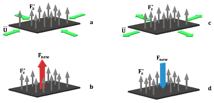
Figure 1: The illustration of the physics caused by the new turbulent heat flux ${\bm{F}}_{\rm new}=-\tau_{0}\,{\bm{F}}_{z}^{\ast}\,{\rm div}\,\overline{\bm{U}}_{\perp}$ produced by the perturbations of the convergent (or divergent) horizontal mean flows $\overline{\bm{U}}_{\perp}$ (shown by the green arrows in panels a and c). The new turbulent flux ${\bm{F}}_{\rm new}$ increases the upward turbulent heat flux, enhances buoyancy and increases the local mean potential temperature, thus creating the upward flow. Likewise, the new turbulent flux ${\bm{F}}_{\rm new}$ decreases the vertical turbulent flux of potential temperature by the divergent horizontal motions, which reduces the buoyancy and decreases the local mean potential temperature, thus creating the downward flow. These effects create the large-scale circulation.

The physics related to the additional terms in the turbulent heat flux is discussed below. The term $\propto-\tau_{0}\,{\bm{F}}_{z}^{\ast}\,{\rm div}\,\overline{\bm{U}}_{\perp}$ in Eq. (3) for the turbulent heat flux causes the redistribution of the vertical background turbulent heat flux ${\bm{F}}_{z}^{\ast}$ by the perturbations of the convergent (or divergent) horizontal mean velocity $\overline{\bm{U}}_{\perp}$ (see Fig. 1) during the life-time of turbulent eddies. As the result, this additional contribution enhances the vertical turbulent flux of potential temperature due to the converging horizontal motions, which increases the buoyancy, thus creating the upward flow. The latter increases the horizontal convergent flow.

On the other hand, the term $\propto(\tau_{0}/2)\,(\overline{\bm{W}}{\bm{\times}}{\bm{F}}_{z}^{\ast})$ in Eq. (3) produces the horizontal turbulent heat flux by the ”rotation” of the vertical background turbulent heat flux ${\bm{F}}_{z}^{\ast}$ caused by the perturbations of the horizontal mean vorticity $\overline{\bm{W}}_{\perp}$. This decreases local potential temperatures in rising motions, which decreases the buoyancy accelerations, and weakens vertical velocity and vorticity.

The last term $\propto(\tau_{0}/2)\,\left(\overline{\bm{W}}_{z}{\bf\times}{\bf F}_{x}^{\rm CW}\right)$ in Eq. (3) for the turbulent heat flux produces the horizontal heat flux through the ”rotation” of the horizontal background counter-wind turbulent heat flux ${\bf F}_{x}^{\rm CW}$ by the vertical component of the mean vorticity. The counter-wind turbulent flux of potential temperature ${\bf F}_{x}^{\rm CW}$ arises due to the following reasons. In a horizontally homogeneous and sheared convective turbulence, the mean shear velocity $\overline{U}^{\rm S}_{x}(z)$ increases with the height, while the mean potential temperature $\overline{\Theta}(z)$ decreases with the height. Uprising fluid particles produce both, positive fluctuations of potential temperature, $\theta>0$ because $\partial\theta/\partial t\propto-({\bm{u}}\cdot\mbox{\boldmath$\nabla$})\overline{\Theta}(z)$, and negative fluctuations of horizontal velocity, $u_{x}<0$ because $\partial u_{x}/\partial t\propto-({\bm{u}}\cdot\mbox{\boldmath$\nabla$})\overline{U}^{\rm S}_{x}(z)$. This creates a negative horizontal turbulent flux of potential temperature, $u_{x}\,\theta<0$. On the other hand, sinking fluid particles create both, negative fluctuations of potential temperature, $\theta<0$, and positive fluctuations of horizontal velocity, $u_{x}>0$, resulting in negative horizontal turbulent flux of potential temperature, $u_{x}\,\theta<0$. Therefore, the net horizontal turbulent flux of potential temperature is negative, ${\bf F}_{x}^{\rm CW}\equiv\langle u_{x}\,\theta\rangle<0$, in spite of a zero horizontal mean temperature gradient. Therefore, the counter-wind turbulent flux of potential temperature modifies the turbulent potential temperature flux caused by the non-uniform mean velocity field. The counter-wind turbulent flux is associated with non-gradient turbulence transport of heat.

The last term $\propto(\tau_{0}/2)\,\overline{\bm{W}}_{z}{\bf\times}{\bf F}_{x}^{\rm CW}$ in Eq. (3), causes generation of the cross-wind horizontal turbulent heat flux by turning the counter-wind horizontal turbulent flux ${\bf F}_{x}^{\rm CW}$ by perturbations of vertical component of the mean vorticity $\overline{\bm{W}}_{z}$ (see Fig. 2). This produces alternating pairs of convergence or divergence cross-wind turbulent heat fluxes, ${\bf F}_{y}^{\rm new}=(\tau_{0}/2)\,\overline{\bm{W}}_{z}{\bf\times}{\bf F}_{x}^{\rm CW}$, resulting alternative warmer or cooler patches which, in turn, cause alternative upward warm and downward cool motions. This is precisely the mechanism of large-scale instability responsible for formation of the large-scale convective rolls stretched along the mean shear and generation of convective-shear waves propagating perpendicular to the convective rolls in the sheared convection [50, 51, 52].

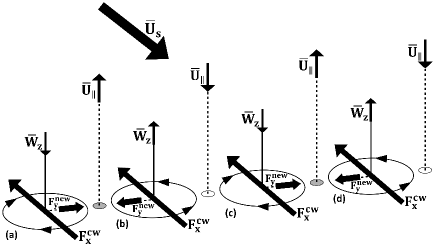
Figure 2: The mechanism of formation of large-scale convective rolls stretched along the shear velocity $\overline{\bm{U}}_{\rm S}(z)$. Horizontal counter-wind turbulent heat flux ${\bf F}_{x}^{\rm CW}$ is turned by perturbations of vertical vorticity $\overline{\bm{W}}_{z}$, i.e., this effect creates alternating pairs of convergence or divergence cross-wind turbulent heat fluxes, ${\bf F}_{y}^{\rm new}=(\tau_{0}/2)\,\overline{\bm{W}}_{z}{\bf\times}{\bf F}_{x}^{\rm CW}$, which are clock-wise or opposite rotations of air columns. This effect causes converging turbulent heat fluxes with warm patch between the pair (a) and (b) of columns in the Figure, and diverging turbulent heat fluxes with cool patch between the pair (b) and (c) in the Figure. The warm patch causes an updraft and cool patch produces a downdraft, whereas the mean shear velocity $\overline{\bm{U}}_{\rm S}(z)$ stretches the flow pattern and completes creation of the large-scale convective rolls.

III Governing equations and convective-shear instability

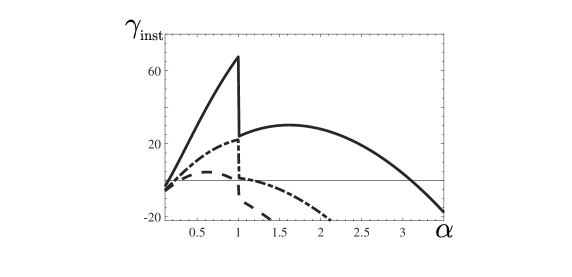
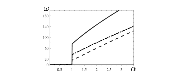
Figure 3: The growth rate $\gamma_{\rm inst}$ of the instability (upper panel) and the frequency of the excited convective-shear waves $\omega$ (bottom panel) versus the parameter $\alpha$ for the effective Rayleigh number ${\rm Ra}_{{}_{T}}=0.5$ and different the non-dimensional shear number ${\rm Sh}=$ 0.03 (dashed); 0.1 (dashed-dotted); 0.3 (solid).

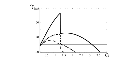
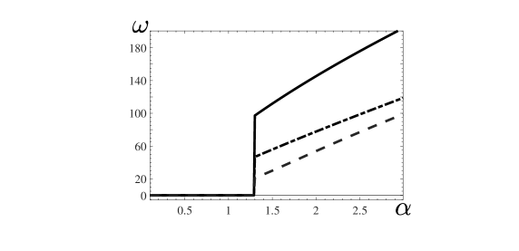
Figure 4: The growth rate $\gamma_{\rm inst}$ of the instability (upper panel) and the frequency of the excited convective-shear waves $\omega$ (bottom panel) versus the parameter $\alpha$ for the effective Rayleigh number ${\rm Ra}_{{}_{T}}=10^{3}$ and different the non-dimensional shear number ${\rm Sh}=$ 0.03 (dashed); 0.1 (dashed-dotted); 0.3 (solid).

Using the expression (3) for the turbulent heat flux ${\bf F}$ with the additional terms caused by the non-uniform mean flows, calculating div ${\bm{F}}$, and assuming that the non-dimensional total vertical heat flux $\Phi_{c}=\tilde{F}_{z}^{\ast}+\tilde{U}_{z}\,\tilde{\Theta}$ is constant, we rewrite Eqs. (1)–(2) in a non-dimensional form as

$${\partial\tilde{\bm{U}}\over\partial t}+(\tilde{\bm{U}}\cdot{\bm{\nabla}})\tilde{\bm{U}}+(\tilde{\bm{U}}_{\rm S}\cdot\mbox{\boldmath$\nabla$})\tilde{\bm{U}}+(\tilde{\bm{U}}\cdot\mbox{\boldmath$\nabla$})\tilde{\bm{U}}_{\rm S}$$

$$\;=-{{\bm{\nabla}}\tilde{P}\over\rho_{0}}+{\rm Ra}_{{}_{T}}\,\tilde{\Theta}\,{\bm{e}}+\Delta\tilde{\bm{U}},$$ (4)

$${\rm Pr}_{{}_{T}}\,\left({\partial\tilde{\Theta}\over\partial t}+\left[\left(\tilde{\bm{U}}+\tilde{\bm{U}}_{\rm S}\right)\cdot{\bm{\nabla}}\right]\tilde{\Theta}\right)=\tilde{U}_{z}+\Delta\tilde{\Theta}$$

$$\;+{\epsilon\over 2}\biggl{\{}\left(\Phi_{c}-\tilde{U}_{z}\,\tilde{\Theta}\right)\,\biggl{[}\left(\Delta-2\nabla_{z}^{2}\right)\tilde{U}_{z}+{\rm Sh}\,\Big{(}\nabla_{y}^{2}\tilde{U}_{x}$$

$$\;-\nabla_{x}\nabla_{y}\tilde{U}_{y}\Big{)}\biggr{]}+2\left(\nabla_{z}\tilde{U}_{z}\right)\nabla_{z}\left(\tilde{U}_{z}\,\tilde{\Theta}\right)+\Big{(}\nabla_{z}\tilde{U}_{x}$$

$$\;-\nabla_{x}\tilde{U}_{z}\Big{)}\,\nabla_{x}\left(\tilde{U}_{z}\,\tilde{\Theta}\right)+\biggl{[}\nabla_{z}\tilde{U}_{y}-\nabla_{y}\tilde{U}_{z}$$

$$\;+{\rm Sh}\,\left(\nabla_{x}\tilde{U}_{y}-\nabla_{y}\tilde{U}_{x}\right)\biggr{]}\,\nabla_{y}\left(\tilde{U}_{z}\,\tilde{\Theta}\right)\biggr{\}},$$ (5)

where the non-dimensional mean velocity $\tilde{\bm{U}}$ with ${\rm div}\,\tilde{\bm{U}}=0$, the mean potential temperature $\tilde{\Theta}$ and the mean pressure $\tilde{P}$ are shown with tilde, the flux $\tilde{F}_{z}^{\ast}$ is the nondimensional vertical turbulent background heat flux, the unit vector ${\bm{e}}$ is directed along vertical $z$ axis, the non-dimensional shear velocity is $\tilde{\bm{U}}_{\rm S}=({\rm Sh}\,\tilde{z},0,0)$, and $\tilde{z}$ is is the non-dimensional vertical coordinate.

Equations (4)–(5) are written in non-dimensional form, where length is measured in the units of the vertical size of the convective layer $L_{z}$, time is measured in the units of the turbulent viscosity time, $L_{z}^{2}/\nu_{{}_{T}}$, velocity is measured in the units of $\nu_{{}_{T}}/L_{z}$, potential temperature is measured in the units of $L_{z}\,N^{2}\,{\rm Pr}_{{}_{T}}/\beta$ and pressure is measured in the units of $\rho_{0}\,(\nu_{{}_{T}}/L_{z})^{2}$. Here $\nu_{{}_{T}}=u_{0}\,\ell_{0}/3$ is the turbulent (eddy) viscosity, $u_{0}$ is the r.m.s. turbulent velocity, $\ell_{0}$ is the turbulent integral scale and $N^{2}=\beta\,|\nabla_{z}\overline{T}_{\rm eq}|$.

We use the following dimensionless parameters appeared in Eqs. (4)–(5):

• the effective Rayleigh number:

  $${\rm Ra}_{{}_{T}}={L_{z}^{4}\,N^{2}\over\nu_{{}_{T}}\,\kappa_{{}_{T}}},$$ (6)

• the turbulent Prandtl number:

  $${\rm Pr}_{{}_{T}}={\nu_{{}_{T}}\over\kappa_{{}_{T}}},$$ (7)

• the scale separation parameter:

  $$\epsilon={\ell_{0}^{2}\over 3L_{z}^{2}},$$ (8)

• the non-dimensional total vertical heat flux:

  $$\Phi_{c}={3\over\epsilon^{2}\,{\rm Ra}_{{}_{T}}}\,\left({u_{c}\over u_{0}}\right)^{3},$$ (9)

• the non-dimensional shear number:

  $${\rm Sh}={S\,\tau_{0}\over\epsilon},$$ (10)

where $S=\nabla_{z}\overline{U}^{\rm S}_{x}$ is the linear velocity shear, i.e., $S$ is constant, $u_{c}=(gF_{z}\ell_{0})^{1/3}$ is the convective velocity, $F_{z}$ is the vertical turbulent flux of potential temperature, $\kappa_{{}_{T}}$ is the turbulent (eddy) diffusivity and $\tau_{0}=\ell_{0}/u_{0}$. In Eqs (4)–(5) we have neglected small terms ${\rm O}(\epsilon^{2})$.

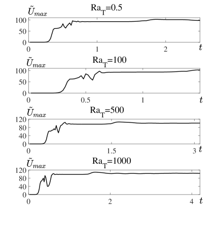
Figure 5: Time evolution of the maximum velocity $\tilde{U}_{\rm max}(t)$ for $\epsilon=10^{-3}$, $\alpha=0.5$ and shear number ${\rm Sh}=1$, and at different values of the effective Rayleigh number ${\rm Ra}_{{}_{T}}=$ 0.5; 100; 500 and 1000 for the stress-free boundary conditions.

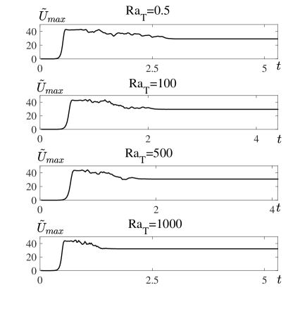
Figure 6: Time evolution of the maximum velocity $\tilde{U}_{\rm max}(t)$ for $\epsilon=10^{-3}$, $\alpha=0.5$ and shear number ${\rm Sh}=1$, and at different values of the effective Rayleigh number ${\rm Ra}_{{}_{T}}=$ 0.5; 100; 500 and 1000 for the no-slip boundary conditions.

For analytical study of the large-scale instability, we consider for simplicity the two-dimensional problem when the mean fields are independent of the coordinate $x$. The non-dimensional shear velocity, $\tilde{\bm{U}}_{\rm S}=({\rm Sh}\,\tilde{z},0,0)$, is directed along the $x$ axis, so that the vorticity $\tilde{\bm{W}}_{\rm S}\equiv{\bm{\nabla}}\times\tilde{\bm{U}}_{\rm S}$ is $\tilde{\bm{W}}_{\rm S}=(0,{\rm Sh},0)$. We will start our analysis with the linear problem for small perturbations applying the linearised Eqs. (4)–(5), to find the growth rate of the large-scale convective-shear instability. To this end, we calculate $[{\bm{\nabla}}\times({\bm{\nabla}}\times\tilde{\bm{U}})]_{z}$ using the linearised Eq. (4) to exclude the pressure term and we seek for solution of the obtained equations in the following form: $\tilde{\bm{U}}(t,{\bm{x}})=\tilde{\bm{U}}_{0}\exp[\gamma t-{\rm i}(K_{y}y+K_{z}z)]$ and $\tilde{\Theta}(t,{\bm{x}})=\Theta_{0}\exp[\gamma t-{\rm i}(K_{y}y+K_{z}z)]$. This yields the following system of algebraic equations:

$$\left(\gamma+K^{2}\right)\,\tilde{U}_{z}+{\rm Ra}_{{}_{T}}\,\left({K_{z}^{2}\over K^{2}}-1\right)\,\tilde{\Theta}=0,$$ (11)

$$\left[1+{\sigma\over 2\epsilon\,{\rm Ra}_{{}_{T}}}\left(2K_{z}^{2}-K^{2}+{{\rm Sh}^{2}K_{y}^{2}\over\gamma+K^{2}}\right)\right]\,\tilde{U}_{z}$$

$$\qquad-\left(\gamma+K^{2}\right)\,\tilde{\Theta}=0,$$ (12)

where $\sigma=3\,(u_{c}/u_{0})^{3}$, $K=(K_{y}^{2}+K_{z}^{2})^{1/2}$, and we consider, for simplicity, the case when the turbulent Prandtl number ${\rm Pr}_{{}_{T}}=1$. Equations (11) and  (12) yield the equation for $\overline{\gamma}=(\gamma+K^{2})/\gamma_{0}$ as

$$\overline{\gamma}^{3}-\overline{\gamma}-{\pi^{2}\,\sigma\,{\rm Sh}^{2}\,\alpha^{4}\over 2\epsilon\gamma_{0}^{3}\,(1+\alpha^{2})}=0,$$ (13)

where

$$\gamma_{0} = {\alpha\over(1+\alpha^{2})^{1/2}}\left[{\rm Ra}_{{}_{T}}+{\pi^{2}\,\sigma\over 2\epsilon}\left(1-\alpha^{2}\right)\right]^{1/2},$$ (14)

$\alpha=K_{y}/K_{z}$ and $K_{z}=\pi$. This implies that $K_{y}=\alpha\pi$ and $K=(K_{y}^{2}+K_{z}^{2})^{1/2}=\pi\,(1+\alpha^{2})^{1/2}$. When

$${\rm Ra}_{{}_{T}}<{\pi^{2}\,\sigma\over 2\epsilon}\left(\alpha^{2}-1\right),$$ (15)

$\gamma_{0}$ is a complex function.

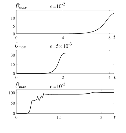
Figure 7: Time evolution of the maximum velocity $\tilde{U}_{\rm max}(t)$ for the effective Rayleigh number ${\rm Ra}_{{}_{T}}=0.5$, $\alpha=0.5$ and shear number ${\rm Sh}=1$, and at different values of the parameter $\epsilon=10^{-3};5\times 10^{-3};10^{-2}$, for the stress-free boundary conditions.

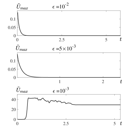
Figure 8: Time evolution of the maximum velocity $\tilde{U}_{\rm max}(t)$ for the effective Rayleigh number ${\rm Ra}_{{}_{T}}=0.5$, $\alpha=0.5$ and shear number ${\rm Sh}=1$, and at different values of the parameter $\epsilon=10^{-3};5\times 10^{-3};10^{-2}$, for the no-slip boundary conditions.

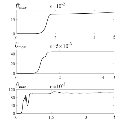
Figure 9: Time evolution of the maximum velocity $\tilde{U}_{\rm max}(t)$ for the effective Rayleigh number ${\rm Ra}_{{}_{T}}=1000$, $\alpha=0.5$ and shear number ${\rm Sh}=1$, and at different values of the parameter $\epsilon=10^{-3};5\times 10^{-3};10^{-2}$, for the stress-free boundary conditions.

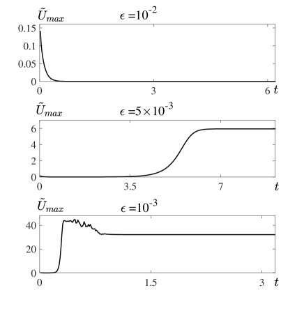
Figure 10: Time evolution of the maximum velocity $\tilde{U}_{\rm max}(t)$ for the effective Rayleigh number ${\rm Ra}_{{}_{T}}=1000$, $\alpha=0.5$ and shear number ${\rm Sh}=1$, and at different values of the parameter $\epsilon=10^{-3};5\times 10^{-3};10^{-2}$, for the no-slip boundary conditions.

Generally, the solution of the cubic equation (13) describes two complex conjugate roots and one real negative root which determine a damping mode. In the case of the complex conjugate roots, the instability can result in an excitation of convective-shear waves with the frequency $\omega={\rm Im}\{\gamma_{0}\,\overline{\gamma}\}$ and the growth rate of the instability $\gamma_{\rm inst}={\rm Re}\{\gamma_{0}\,\overline{\gamma}\}-\pi^{2}(1+\alpha^{2})$, where ${\rm Re}\{Z\}$ is the real part of the complex number and ${\rm Im}\{Z\}$ is the imagine part of the complex number.

Numerical solution of Eq. (13) yields the growth rate $\gamma_{\rm inst}$ of the instability and the frequency $\omega$ of the excited convective-shear waves versus the parameter $\alpha$ for the effective Rayleigh numbers ${\rm Ra}_{{}_{T}}=0.5$ (see upper panel in Fig. 3) and ${\rm Ra}_{{}_{T}}=10^{3}$ (see upper panel in Fig. 4), and for different values of the non-dimensional shear number ${\rm Sh}$. It shows that the convective-shear waves are excited for $\alpha>1$ at small effective Rayleigh numbers and for $\alpha>1.3$ at large effective Rayleigh numbers. The growth rate of the instability and the frequency of the excited convective-shear waves are very weakly dependent on the effective Rayleigh numbers. Increase of shear, results in increase of the growth rate $\gamma_{\rm inst}$ of the instability and the frequency of the excited convective-shear waves $\omega$. The asymptotic solution of Eq. (13) in the case of $\gamma_{\rm inst}\gg\gamma_{0}$ reads

$$\gamma_{\rm inst}=\left({\pi^{2}\,\sigma\,{\rm Sh}^{2}\,\alpha^{4}\over 2\epsilon^{3}\,(1+\alpha^{2})}\right)^{1/3}-\pi^{2}\,(1+\alpha^{2}),$$ (16)

which corresponds to a non-oscillatory growing solution with $\omega=0$.

This instability causes formation of large-scale fluid motions in the form of rolls stretched along the imposed mean wind. This mechanism can also cause the generation of the convective-shear waves with the frequency shown in bottom panels of Figs. 3–4. The convective-shear waves propagate perpendicular to convective rolls. The predicted motions in convective rolls are characterised by nonzero helicity, in agreement with numerical simulations (see Ref. [28]). Note that similar waves propagating in the direction normal to cloud streets (convective rolls) have been detected in atmospheric convective boundary layers (see Ref. [31]). This large-scale instability are fed by the energy of the convective turbulence.

IV Results of mean-field numerical simulations

In this section, we discuss results of mean-field numerical simulations for three-dimensional problem. We solve numerically Eqs. (4)–(5) for the periodic boundary conditions in the horizontal $xy$ plane. The boundary conditions for the potential temperature in the vertical direction are $\tilde{\Theta}(t,z=0)=\tilde{\Theta}(t,z=1)=0$. We use the stress-free and no-slip boundary conditions for the velocity field in the vertical direction (along the $z$ axis). The stress-free boundary conditions imply,

$$\tilde{U}_{z}(t,z=0)=\tilde{U}_{z}(t,z=1)=0,$$ (17)

$$\nabla_{z}\tilde{U}_{x}(t,z=0)=\nabla_{z}\tilde{U}_{x}(t,z=1)=0,$$ (18)

$$\nabla_{z}\tilde{U}_{y}(t,z=0)=\nabla_{z}\tilde{U}_{y}(t,z=1)=0,$$ (19)

while the no-slip boundary conditions are given by

$$\tilde{\bm{U}}(t,z=0)=\tilde{\bm{U}}(t,z=1)=0.$$ (20)

We use the ANSYS FLUENT code (version 19.2) in the $3D$ box $L_{x}=5$ and $L_{y}=L_{z}=1$, which is based on the final volume method. The simulations are performed with the spatial resolution, $500\times 100\times 100$ points in $x$, $y$ and $z$ directions, respectively. In the mean-field numerical simulations, we use the following values of the basic dimensionless parameters: the turbulent Prandtl number ${\rm Pr}_{{}_{T}}=1$, the ratio $u_{c}/u_{0}=1$, the effective Rayleigh number changies from ${\rm Ra}_{{}_{T}}=0.5$ to ${\rm Ra}_{{}_{T}}=1800$ and the scale separation parameter $\epsilon$ varies from $\epsilon=10^{-3}$ to $\epsilon=10^{-2}$. The non-dimensional shear number ${\rm Sh}$ varies from ${\rm Sh}=0.01$ to ${\rm Sh}=1$.

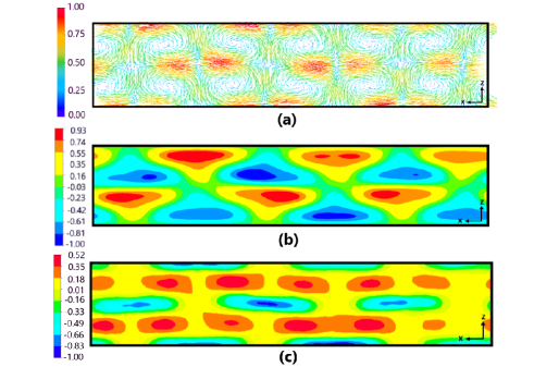
Figure 11: The counter lines of the velocity field (upper panel); the patterns of the potential temperature deviations $\tilde{\Theta}\,{\rm Ra}_{{}_{T}}$ from the equilibrium potential temperature in the basic reference state (middle panel); the patterns of the vertical gradient of the mean potential temperature $(\nabla_{z}\tilde{\Theta}-1)\,{\rm Ra}_{{}_{T}}$ (bottom panel) at time instant $t=0.34$ of the turbulent viscosity time $L_{z}^{2}/\nu_{{}_{T}}$, effective Rayleigh number ${\rm Ra}_{{}_{T}}=0.5$, $\epsilon=10^{-3}$, $\alpha=0.5$ and shear number ${\rm Sh}=1$ for the stress-free vertical boundary conditions. All quantities are normalized by their maximum values.

For illustration, in Figs. 5 and 6 we plot the time evolution of the maximum velocity $\tilde{U}_{\rm max}(t)$ for different values of the effective Rayleigh numbers ${\rm Ra}_{{}_{T}}$ changing from $0.5$ to $10^{3}$ at a fixed value of the parameter $\epsilon$ in the sheared large-scale convection (for ${\rm Sh}=1$), while in Figs. 7–10 we show the time evolution of the maximum velocity $\tilde{U}_{\rm max}(t)$ for different values of the scale separation parameter $\epsilon$ (from $10^{-3}$ to $10^{-2}$) between the vertical size $L_{z}$ of the computational domain and the integral turbulence scale $\ell_{0}$ (see Figs. 7–8 for ${\rm Ra}_{{}_{T}}=0.5$ and Figs. 9–10 for ${\rm Ra}_{{}_{T}}=10^{3}$).

As can be seen in Figs. 5–10, at the initial stage of the evolution, the maximum velocity $\tilde{U}_{\rm max}(t)$ increases in time exponentially due to the excitation of the large-scale convective-shear instability. During the nonlinear stage of the instability, we observe that $\tilde{U}_{\rm max}(t)$ reaches the maximum value which is weakly dependent on the effective Rayleigh number ${\rm Ra}_{{}_{T}}$ for the stress-free and no-slip boundary conditions (see Figs. 5–6). On the other hand, the maximum value of the function $\tilde{U}_{\rm max}$ at the stationary stage strongly depends on the scale separation parameter $\epsilon$ and on the boundary conditions (see Figs. 7–8). In particular, increasing the scale separation between the vertical size $L_{z}$ of the computational domain and the integral turbulence scale $\ell_{0}$ (i.e., decreasing the parameter $\epsilon$), we observe that the maximum value of the function $\tilde{U}_{\rm max}$ increases. For the no-slip vertical boundary conditions, the large-scale instability is excited and convective structures are formed when $\epsilon<3\times 10^{-3}$ at ${\rm Ra}_{{}_{T}}=0.5$, $\epsilon<4\times 10^{-3}$ at ${\rm Ra}_{{}_{T}}=500$ and $\epsilon<7\times 10^{-3}$ at ${\rm Ra}_{{}_{T}}=10^{3}$. In addition, the time evolution in the nonlinear stage of the instability for the stress-free and no-slip boundary conditions are different.

Some features in the time evolution of the maximum velocity $\tilde{U}_{\rm max}(t)$ have been also observed in the recent mean-field simulations of the shear-free convection (see Ref. [53]), where $\tilde{U}_{\rm max}(t)$ is independent of ${\rm Ra}_{{}_{T}}$ for the same boundary conditions, but it strongly depends on the scale separation parameter $\epsilon$. However, in a sheared large-scale convection, we do not observe clear nonlinear oscillations of $\tilde{U}_{\rm max}$ which have been seen after the steady-state stage (when the function $\tilde{U}_{\rm max}$ is nearly constant in time) in the large-scale shear-free convection (see Ref. [53]).

To observe spatial structure of the basic characteristics of the sheared large-scale convection, in Figs. 11–15 we plot the counter lines of the velocity field (upper panels); the patterns of the potential temperature deviations $\tilde{\Theta}\,{\rm Ra}_{{}_{T}}$ from the equilibrium potential temperature in the basic reference state (middle panels) and the patterns of the vertical gradient of the mean potential temperature $(\nabla_{z}\tilde{\Theta}-1)\,{\rm Ra}_{{}_{T}}$ (bottom panels) at several time instants: before the system reaches steady-state (see Figs. 11 and 12) and after the system reaches steady-state (see Fig. 13–15).

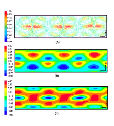
Figure 12: The counter lines of the velocity field (upper panel); the patterns of the potential temperature deviations $\tilde{\Theta}\,{\rm Ra}_{{}_{T}}$ from the equilibrium potential temperature in the basic reference state (middle panel); the patterns of the vertical gradient of the mean potential temperature $(\nabla_{z}\tilde{\Theta}-1)\,{\rm Ra}_{{}_{T}}$ (bottom panel) at time instant $t=0.7$ of the turbulent viscosity time $L_{z}^{2}/\nu_{{}_{T}}$, effective Rayleigh number ${\rm Ra}_{{}_{T}}=0.5$, $\epsilon=10^{-3}$, $\alpha=0.5$ and shear number ${\rm Sh}=1$ for the no-slip vertical boundary conditions. All quantities are normalized by their maximum values.

We remind that the potential temperature is measured in the units of $L_{z}\,N^{2}\,{\rm Pr}_{{}_{T}}/\beta={\rm Ra}_{{}_{T}}\nu_{{}_{T}}^{2}/(\beta L_{z}^{3})$. This is the reason why we show in Figs. 11–15 (see middle panels) the pattern of the normalized deviations of the potential temperature $\tilde{\Theta}\,{\rm Ra}_{{}_{T}}$ from the equilibrium potential temperature in the basic reference state. Note also that the total gradient of the potential temperature is the sum of the equilibrium constant gradient of the potential temperature $\nabla_{z}\overline{T}_{\rm eq}$ (negative for a convection) and the gradient of the potential temperature $\nabla_{z}\overline{\Theta}$. Therefore, we show in Figs. 11–15 (see bottom panels) the pattern of the normalized total vertical gradient of the mean potential temperature, $(\nabla_{z}\tilde{\Theta}-1)\,{\rm Ra}_{{}_{T}}$ which characterises the large-scale convection.

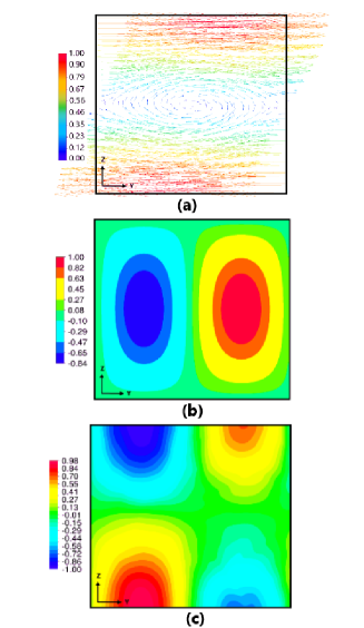
Figure 16: The counter lines of the velocity field (upper panel); the patterns of the potential temperature deviations $\tilde{\Theta}\,{\rm Ra}_{{}_{T}}$ from the equilibrium potential temperature in the basic reference state (middle panel); the patterns of the vertical gradient of the mean potential temperature $(\nabla_{z}\tilde{\Theta}-1)\,{\rm Ra}_{{}_{T}}$ (bottom panel) at time instant $t=0.04$ of the turbulent viscosity time $L_{z}^{2}/\nu_{{}_{T}}$, effective Rayleigh number ${\rm Ra}_{{}_{T}}=0.5$, $\epsilon=10^{-3}$, $\alpha=0.5$ and shear number ${\rm Sh}=1$ for the no-slip vertical boundary conditions. All quantities are normalized by their maximum values.

At the linear stage of the system evolution, the patterns for the stress-free and no-slip boundary conditions are the same (see Fig. 16). During the evolution, there is a transition from the large-scale circulations at the $yz$ plane seen in the linear stage of the instability (see Fig. 16) to the the large-scale circulations at the $xz$ plane observed during nonlinear stage of the instability (see Figs. 11–12). In addition, there is a transition from the two-layer vertical structure of the mean velocity field with two convective roles in the $z$ direction and six roles in the $x$ direction (as can be seen in Fig. 11 for the stress-free boundary conditions) to the one-layer vertical structure with one role in the $z$ direction and two roles in the $x$ direction (see Fig. 13).

On the other hand, comparing Figs. 12 and 14 (which corresponds to the no-slip boundary conditions), we observe that during nonlinear stage of the instability there is a transition from the large-scale circulations with the two-layer vertical structure with two convective roles in the $z$ direction and six roles in the $x$ direction (see Fig. 12) to the one-layer structure with four inclined roles (see Fig. 14). The formation of the inclined roles for the no-slip boundary conditions are already observed starting with $t=0.9$ of the turbulent viscosity time $L_{z}^{2}/\nu_{{}_{T}}$ at the effective Rayleigh number ${\rm Ra}_{{}_{T}}=0.5$. The inclined roles for the no-slip boundary conditions are also observed at the effective Rayleigh number ${\rm Ra}_{{}_{T}}=10^{3}$ (see Fig. 15).

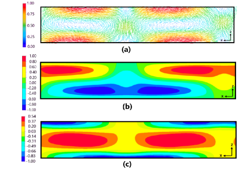
Figure 13: The counter lines of the velocity field (upper panel); the patterns of the potential temperature deviations $\tilde{\Theta}\,{\rm Ra}_{{}_{T}}$ from the equilibrium potential temperature in the basic reference state (middle panel); the patterns of the vertical gradient of the mean potential temperature $(\nabla_{z}\tilde{\Theta}-1)\,{\rm Ra}_{{}_{T}}$ (bottom panel) at time instant $t=1$ of the turbulent viscosity time $L_{z}^{2}/\nu_{{}_{T}}$, effective Rayleigh number ${\rm Ra}_{{}_{T}}=0.5$, $\epsilon=10^{-3}$, $\alpha=0.5$ and shear number ${\rm Sh}=1$ for the stress-free vertical boundary conditions. All quantities are normalized by their maximum values.

As has been observed in the shear-free convection [53], the large-scale convective structures are also formed in a sheared convection even at low values of the effective Rayleigh numbers ${\rm Ra}_{{}_{T}}=0.5$ due to the additional terms $\propto\epsilon$ in Eq. (5) for the evolution of the potential temperature (which are caused by the modification of the turbulent heat flux by non-uniform fluid flows). Moreover, in Figs. 11–15 (bottom panels), one can see the regions with the positive gradient of the potential temperature $(\nabla_{z}\tilde{\Theta}-1)\,{\rm Ra}_{{}_{T}}$, which are typical for stably stratified turbulence. Such effects have been previously observed in experiments [16, 54], direct numerical simulations [44, 46, 55, 47] of turbulent convection and shear-free mean-field numerical simulations [53]. The formation of the regions with the positive gradient of the potential temperature inside the large-scale circulation can be understood as follows. The total vertical heat flux ${\bm{F}}_{z}^{\rm tot}$ includes three contributions [53]:

• the mean vertical heat flux $\overline{\bm{U}}_{z}\,\overline{\Theta}$ of the large-scale circulation,

• the vertical turbulent heat flux ${\bm{F}}_{z}^{\ast}=-\kappa_{{}_{T}}{\bm{\nabla}}_{z}\overline{\Theta}$, and

• the new turbulent heat flux ${\bm{F}}_{z}^{\rm new}=-\tau_{0}\,{\bm{F}}_{z}^{\ast}\,{\rm div}\,\overline{\bm{U}}_{\perp}$.

Therefore, the vertical gradient $\nabla_{z}\overline{\Theta}$ of the mean potential temperature is given by

$$\nabla_{z}\overline{\Theta}={\overline{U}_{z}\,\overline{\Theta}-F_{z}^{\rm tot}\over\kappa_{{}_{T}}\,(1-\tau_{0}\,{\rm div}\,\overline{\bm{U}}_{\perp})}.$$ (21)

Inside the large-scale circulation where $\overline{U}_{z}\,\overline{\Theta}>F_{z}^{\rm tot}$, the vertical gradient $\nabla_{z}\overline{\Theta}$ is positive. On the other hand, when $\overline{U}_{z}\,\overline{\Theta}<F_{z}^{\rm tot}$, the vertical gradient $\nabla_{z}\overline{\Theta}$ is negative. Here we take into account that $\tau_{0}\,|{\rm div}\,\overline{\bm{U}}_{\perp}|<1$.

In the present study, we also observe the formation the large-scale rolls even below the threshold of the laminar convection (see Figs. 11–14 for effective Rayleigh number ${\rm Ra}_{{}_{T}}=0.5$ which can be compared with Fig. 15 for ${\rm Ra}_{{}_{T}}=1000$). This is because turbulence with non-uniform large-scale flows contributes to the turbulent heat flux. The reasons for this effect are related to production of additional essentially anisotropic velocity fluctuations generated by tangling of the mean-velocity gradients by small-scale turbulent motions due to the influence of the inertial forces during the lifetime of turbulent eddies. These anisotropic velocity fluctuations contributes to the turbulent heat flux. As the result of this effect, there is an excitation of large-scale convective-shear instability, which results in the formation of large-scale semi-organized structures in the form of rolls and generation of convective-shear waves propagating perpendicular to the convective rolls. The life-times and spatial scales of these structures are much larger compared to the largest turbulent time scales. As the result, the evolutionary equation (5) for the potential temperature $\tilde{\Theta}$ contains the new terms proportional to the spatial derivatives of the mean velocity field $\tilde{\bm{U}}$ (see the terms $\propto\epsilon$).

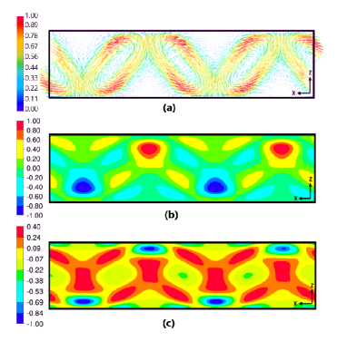
Figure 14: The counter lines of the velocity field (upper panel); the patterns of the potential temperature deviations $\tilde{\Theta}\,{\rm Ra}_{{}_{T}}$ from the equilibrium potential temperature in the basic reference state (middle panel); the patterns of the vertical gradient of the mean potential temperature $(\nabla_{z}\tilde{\Theta}-1)\,{\rm Ra}_{{}_{T}}$ (bottom panel) at time instant $t=4$ of the turbulent viscosity time $L_{z}^{2}/\nu_{{}_{T}}$, effective Rayleigh number ${\rm Ra}_{{}_{T}}=0.5$, $\epsilon=10^{-3}$, $\alpha=0.5$ and shear number ${\rm Sh}=1$ for the no-slip vertical boundary conditions. All quantities are normalized by their maximum values.

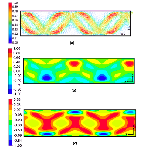
Figure 15: The counter lines of the velocity field (upper panel); the patterns of the potential temperature deviations $\tilde{\Theta}\,{\rm Ra}_{{}_{T}}$ from the equilibrium potential temperature in the basic reference state (middle panel); the patterns of the vertical gradient of the mean potential temperature $(\nabla_{z}\tilde{\Theta}-1)\,{\rm Ra}_{{}_{T}}$ (bottom panel) at time instant $t=5.32$ of the turbulent viscosity time $L_{z}^{2}/\nu_{{}_{T}}$, effective Rayleigh number ${\rm Ra}_{{}_{T}}=1000$, $\epsilon=10^{-3}$, $\alpha=0.5$ and shear number ${\rm Sh}=1$ for the no-slip vertical boundary conditions. All quantities are normalized by their maximum values.

V Conclusions

Mean-field simulations based on a developed mean-field theory [50, 51] of a non-rotating sheared turbulent convection are performed. This mean-field theory describes an effect of modification of the turbulent heat flux by the non-uniform large-scale motions caused by production of essentially anisotropic velocity fluctuations generated by tangling of the mean-velocity gradients by small-scale turbulent motions. The effect causes an excitation of large-scale convective-shear instability and the formation of large-scale convective rolls. During the nonlinear stage of the convective-shear instability, there is a transition from the two-layer vertical structure with two roles in the vertical direction before the system reaches steady-state to the one-layer vertical structure with one role after the system reaches steady-state. This effect is observed for all effective Rayleigh numbers.

The performed mean-field simulations show that the modification of the turbulent heat flux by the non-uniform large-scale motions results in a strong decrease of the critical effective Rayleigh number required for the formation of the large-scale rolls. These mean-field simulations have demonstrated that the spatial distribution of the mean potential temperature has regions with a positive vertical gradient of the potential temperature inside the convective roll due to the mean heat flux of the convective rolls. This study might be useful for understanding the origin of large-scale rolls observed in atmospheric convective boundary layers as well as in numerical simulations and laboratory experiments.

DATA AVAILABILITY

The data that support the findings of this study are available from the corresponding author upon reasonable request.

AUTHOR DECLARATIONS

Conflict of Interest

The authors have no conflicts to disclose.

References

- [1] S. Chandrasekhar, Hydrodynamic and Hydromagnetic Stability (Oxford Univ. Press, Oxford, 1961).
- [2] J. S. Turner, Buoyancy Effects in Fluids (Cambridge University Press, Cambridge, 1973).
- [3] S. S. Zilitinkevich, Turbulent Penetrative Convection (Avebury Technical, Aldershot, 1991).
- [4] E. Bodenschatz, W. Pesch, and G. Ahlers, Recent developments in Rayleigh-Bénard convection, Annu. Rev. Fluid Mech. 32, 709 (2000).
- [5] G. Ahlers, S. Grossmann, D. Lohse, Heat transfer and large scale dynamics in turbulent Rayleigh-Bénard convection, Rev. Mod. Phys. 81, 503 (2009).
- [6] D. Lohse, K.-Q. Xia, Small-scale properties of turbulent Rayleigh-Bénard convection, Annu. Rev. Fluid Mech. 42, 335 (2010).
- [7] Q. Zhou and K.-Q. Xia, The mixing evolution and geometric properties of a passive scalar field in turbulent Rayleigh–Bénard convection, New J. Physics 12, 083029 (2010).
- [8] A. S. Monin and A. M. Yaglom, Statistical Fluid Mechanics (Dover, New York, 2013).
- [9] M. Lesieur, Turbulence in Fluids (Springer, Dordrecht, 2008).
- [10] P. A. Davidson, Turbulence in Rotating, Stratified and Electrically Conducting Fluids (Cambridge University Press, Cambridge, 2013).
- [11] E. S. C. Ching, Statistics and Scaling in Turbulent Rayleigh-Bénard Convection (Springer, Singapore, 2014).
- [12] I. Rogachevskii, Introduction to Turbulent Transport of Particles, Temperature and Magnetic Fields (Cambridge University Press, Cambridge, 2021).
- [13] R. Krishnamurti and L. N. Howard, Large-scale flow generation in turbulent convection, Proc. Natl.Acad. Sci. USA 78, 1981 (1981).
- [14] M. Sano, X. Z. Wu and A. Libchaber, Turbulence in helium-gas free convection, Phys. Rev. A 40, 6421 (1989).
- [15] S. Ciliberto, S. Cioni and C. Laroche, Large-scale flow properties of turbulent thermal convection, Phys. Rev. E 54, R5901 (1996).
- [16] J. J. Niemela, L. Skrbek, K. R. Sreenivasan and R. J. Donnelly, The wind in confined thermal convection, J. Fluid Mech. 449, 169 (2001).
- [17] J. J. Niemela and K. R. Sreenivasan, Rayleigh-number evolution of large-scale coherent motion in turbulent convection, Europhys. Lett. 62, 829 (2003).
- [18] U. Burr, W. Kinzelbach, A. Tsinober, Is the turbulent wind in convective flows driven by fluctuations?, Phys. Fluids 15, 2313 (2003).
- [19] H. D. Xi, S. Lam and X. Q. Xia, From laminar plumes to organized flows: the onset of large-scale circulation in turbulent thermal convection, J. Fluid Mech. 503, 47 (2004).
- [20] D. Funfschilling and G. Ahlers, Plume motion and large-scale circulation in a cylindrical Rayleigh-Bénard cell, Phys. Rev. Lett. 92, 194502 (2004).
- [21] E. Brown, A. Nikolaenko and G. Ahlers, Orientation changes of the large-scale circulation in turbulent Rayleigh-Bénard convection, Phys. Rev. Lett. 95, 084503 (2005).
- [22] A. Liberzon, B. Lüthi, M. Guala, W. Kinzelbach and A. Tsinober, Experimental study of the structure of flow regions with negative turbulent kinetic energy production in confined three-dimensional shear flows with and without buoyancy, Phys. Fluids 17, 095110 (2005).
- [23] A. Eidelman, T. Elperin, N. Kleeorin, A. Markovich and I. Rogachevskii, Hysteresis phenomenon in turbulent convection, Experim. Fluids 40, 723 (2006).
- [24] D. Funfschilling, E. Brown and G. Ahlers, Torsional oscillations of the large-scale circulation in turbulent Rayleigh-Bénard convection, J. Fluid Mech 607, 119 (2008).
- [25] M. Bukai, A. Eidelman, T. Elperin, N. Kleeorin, I. Rogachevskii and I. Sapir-Katiraie, Effect of large-scale coherent structures on turbulent convection, Phys. Rev. E 79, 066302 (2009).
- [26] M. Bukai, A. Eidelman, T. Elperin, N. Kleeorin, I. Rogachevskii and I. Sapir-Katiraie, Transition phenomena in unstably stratified turbulent flows, Phys. Rev. E 83, 036302 (2011).
- [27] J. C. Kaimal and J. J. Fennigan, Atmospheric Boundary Layer Flows (Oxford University Press, New York, 1994).
- [28] D. Etling, Some aspects on helicity in atmospheric flows, Contrib. Atmos. Physics 58, 88 (1985).
- [29] D. Etling and R. A. Brown, Roll vortices in the planetary boundary layer: a review, Boundary-Layer Meteorol. 65, 215 (1993).
- [30] B. W. Atkinson and J. Wu Zhang, Mesoscale shallow convection in the atmosphere, Rev. Geophys. 34, 403 (1996).
- [31] B. Brümmer, Roll and cell convection in winter-time arctic cold-air outbreaks, J. Atmosph. Sci. 56, 2613 (1999).
- [32] G. S. Young, D. A. R. Kristovich, M. R. Hjelmfelt and R. C. Foster, Rolls, streets, waves and more, BAMS, July, ES54 (2002).
- [33] J. C. Wyngaard, Turbulence in the Atmosphere (Cambridge University Press, 2010).
- [34] F. Tampieri, Turbulence and Dispersion in the Planetary Boundary Layer (Springer, 2017).
- [35] B. Jayaraman and J. G. Brasseur, Transition in atmospheric boundary layer turbulence structure from neutral to convective, and large-scale rolls, J. Fluid Mech. 913, A42 (2021).
- [36] S. Zilitinkevich, E. Kadantsev, I. Repina, E. Mortikov, and A. Glazunov, “Order out of chaos: Shifting paradigm of convective turbulence,” J. Atmos. Sci. 78, 3925 (2021).
- [37] I. Rogachevskii, N. Kleeorin, and S. Zilitinkevich, Energy-and flux-budget theory for surface layers in atmospheric convective turbulence, Phys. Fluids 34, 116602 (2022).
- [38] I. Rogachevskii and N. Kleeorin, Semi-organized structures and turbulence in the atmospheric convection, Phys. Fluids 36, 026610 (2024).
- [39] T. Hartlep, A. Tilgner and F. H. Busse, Large-scale structures in Rayleigh-Benard convection at high Rayleigh numbers, Phys. Rev. Lett. 91, 064501 (2003).
- [40] A. Parodi, J. von Hardenberg, G. Passoni, A. Provenzale and E. A. Spiegel, Clustering of plumes in turbulent convection, Phys. Rev. Lett. 92, 194503 (2004).
- [41] F. Rincon, Anisotropy, inhomogeneity and inertial-range scalings in turbulent convection, J. Fluid Mech. 563, 43 (2006).
- [42] J. Schumacher, Lagrangian dispersion and heat transport in convective turbulence, Phys. Rev. Lett. 100 134502 (2008).
- [43] F. Chillà, J. Schumacher, New perspectives in turbulent Rayleigh-Bénard convection, Eur. Phys. J. E 35, 58 (2012).
- [44] A. Brandenburg, Stellar mixing length theory with entropy rain, Astrophys. J. 832, 6 (2016).
- [45] A. Hellsten and S. Zilitinkevich, Role of convective structures and background turbulence in the dry convective boundary layer, Boundary-Layer Meteorol. 149, 323 (2013).
- [46] P. J. Käpylä, M. Rheinhardt, A. Brandenburg, R. Arlt, M. J. Käpylä, A. Lagg, N. Olspert, J. Warnecke, Extended subadiabatic layer in simulations of overshooting convection, Astrophys. J. Lett. 845, L23 (2017).
- [47] P. J. Käpylä, Overshooting in simulations of compressible convection, Astron. Astrophys. 631, A122 (2019).
- [48] J. Schumacher and K. R. Sreenivasan, Colloquium: Unusual dynamics of convection in the Sun, Rev. Mod. Phys. 92, 041001 (2020).
- [49] A. Pandey, J. Schumacher and K. R. Sreenivasan, Non-Boussinesq low-Prandtl-number convection with a temperature-dependent thermal diffusivity, Astrophys. J. 907, 56 (2021).
- [50] T. Elperin, N. Kleeorin, I. Rogachevskii and S.S. Zilitinkevich, Formation of large-scale semi-organized structures in turbulent convection, Phys. Rev. E 66, 066305 (2002).
- [51] T. Elperin, N. Kleeorin, I. Rogachevskii and S.S. Zilitinkevich, Tangling turbulence and semi-organized structures in convective boundary layers, Boundary-Layer Meteorology 119, 449-472 (2006).
- [52] T. Elperin, I. Golubev, N. Kleeorin, I. Rogachevskii, Large-scale instabilities in a nonrotating turbulent convection, Phys. Fluids 18, 126601 (2006).
- [53] G. Orian, A. Asulin, E. Tkachenko, N. Kleeorin, A. Levy, and Rogachevskii I., Large-scale circulations in a shear-free convective turbulence: Mean-field simulations, Phys. Fluids 34, 105121 (2022).
- [54] L. Barel, A. Eidelman, T. Elperin, G. Fleurov, N. Kleeorin, A. Levy, I. Rogachevskii and O. Shildkrot, Detection of standing internal gravity waves in experiments with convection over a wavy heated wall, Phys. Fluids 32, 095105 (2020).
- [55] S. Toppaladoddi, S. Succi, and J. S. Wettlaufer, Roughness as a route to the ultimate regime of thermal convection, Phys. Rev. Lett. 118, 074503 (2017).