Photon blockade in non-Hermitian optomechanical systems with nonreciprocal couplings
Abstract
We study the photon blockade at exceptional points for a non-Hermitian optomechanical system coupled to the driven whispering-gallery-mode microresonator with two nanoparticles under the weak optomechanical coupling approximation, where exceptional points emerge periodically by controlling the relative angle of the nanoparticles. We find that conventional photon blockade occurs at exceptional points for the eigenenergy resonance of the single-excitation subspace driven by a laser field, and discuss the physical origin of conventional photon blockade. Under the weak driving condition, we analyze the influences of the different parameters on conventional photon blockade. We investigate conventional photon blockade at non-exceptional points, which exists at two optimal detunings due to the eigenstates in the single-excitation subspace splitting from one (coalescence) at exceptional points to two at non-exceptional points. Unconventional photon blockade can occur at non-exceptional points, while it does not exist at exceptional points since the destructive quantum interference cannot occur due to the two different quantum pathways to the two-photon state being not formed. The realization of photon blockade in our proposal provides a viable and flexible way for the preparation of single-photon sources in the non-Hermitian optomechanical system.
I Introduction
Photon blockade (PB) and tunneling are current research topics and play an essential role in various fundamental studies and practical applications Bajcsy15025014 ; Bamba99171111 ; Carusotto85299 ; Ferretti82013841 ; Ferretti15025012 ; Ferretti85033303 ; Flayac88033836 ; Gerace89031803 ; Greentree2252 ; Gheri602673 ; Imamoglu791467 ; Kyriienko90063805 ; Majumdar21160 ; Majumdar87235319 ; Rebic65063804 ; Zhou92023838 ; Giovannetti222 ; Knill46 ; Kok135 ; Li053837 ; Wang053832 ; Shen023805 ; Ren053710 ; Stefanatos013716 . In these pioneering studies, PB is generated in weakly nonlinear systems, allowing for destructive quantum interference between distinct driven-dissipative pathways Liew104183601 ; Bamba83021802 ; Flayac96053810 ; Carmichael2790 ; Casalengua1900279 ; Kyriienko033807 , called unconventional PB (UPB). Based on this fundamental principle, many quantum systems are predicted to have PB effect with weak nonlinearities, such as the nonlinear photonic molecule Xu90043822 ; Xu033832 ; Xu033809 , optical cavity with a quantum dot Zhang043832 ; Tang9252 ; Liang053713 ; Wang64003 , coupled single-mode cavities with second- or third-order nonlinearity Flayac013815 ; Flayac11223 ; Shen32835 ; Shen035503 ; Zhou17332 ; Zou16175 ; Roberts021022 , coupled optomechanical system Xu035502 ; Savona5937 ; Qu043823 ; Hou063817 , a gain cavity Zhou043819 , exciting polaritons Carreno196402 , non-Markovian system shen023856 ; Shen013826 , and Gaussian squeezed states Lemonde90063824 ; Sarma053827 . On the other hand, PB arises from the anharmonicity in the eigenenergy of the systems caused by strong nonlinearity Huang121153601 ; Birnbaum87 ; Shen023849 ; Zhou033713 ; Lee013834 ; Kim397500 ; Smolyaninov187402 ; Zheng107223601 ; Majumdar183601 , called conventional PB (CPB). There are various systems for producing CPB, such as cavity quantum electrodynamics (QED) systems Hennrich94053604 ; Hamsen118133604 ; Ridolfo109193602 ; Tian6801 ; Werner011801 ; Brecha2392 ; Rebic490 ; Liang063834 ; Yan5086 ; Fink011012 ; Miranowicz023809 ; Zhu063842 ; Faraon033838 ; Liao053836 ; Lin053850 , circuit QED systems Lang106243601 ; Hoffman107053602 ; Liu89043818 ; Leib093031 , optomechanical systems Rabl107063601 ; Wang92033806 ; Zhai07654 ; Nunnenkamp063602 ; Liao023853 ; Komar013839 ; Lu2943 ; Xu013818 ; Miranowicz013808 ; Xie063860 ; Xie013861 ; Zou043837 ; Liu032101 , coupled cavities Angelakis76031805 ; Shen91063808 , a two-level system coupled to the cavity Grujic103025 ; Boite033827 ; Radulaski011801 ; Li043724 ; Xue4424 ; Jing033707 ; Yao054004 , dynamical blockade Ghosh013602 , a quantum dot in a photonic crystal system Faraon859 , and a quantum dot coupled to a nanophotonic waveguide Foster173603 .
Experimentally Vaneph043602 ; Snijders043601 , the signature of PB and tunneling can be distinguished by measuring the second-order correlation function Loudon2000 . For the PB (or the photon antibunching ), driven by an external coherent field, the presence of a single photon in a system will hinder the coupling of the subsequent photons because of the strong nonlinearities presenting in the quantum system, while for the photon tunneling (or the photon bunching ), the coupling of initial photons will favor the coupling of the subsequent photons Loudon2000 . The potential applications of PB include the realizations of interferometers Gerace281 , quantum nonreciprocity Fratini243601 ; Mascarenhas54003 , and single-photon transistors Chang807 .
The nonlinear interaction between optical and mechanical modes arising from the radiation pressure force in cavity optomechanical (COM) systems exhibits many interesting nonlinear effects such as photon (phonon) blockade Rabl107063601 ; Ramos110193602 ; Wang093006 , nonreciprocity Xu143 ; Manipatruni213903 ; Shen657 ; Bernier604 ; Jiang064037 ; Li630 ; Liu15382 ; Shang115202 ; Gao25161 ; Xu053854 ; Mirza25515 ; Jiao143605 , optomechanical-induced transparency Agarwal81041803 ; Teufel471204 ; Zhang025199 , and nonlinearity Aldana88043826 ; Zhou88063854 ; Lu093602 . Cavity optomechanics has received significant attention in both fundamental experiments Teufel475359 ; Chan47889 and sensing applications Abbott11073032 ; Pontin89023848 . Currently, experimental techniques of cavity optomechanics are still in the single-photon weak-coupling regime Aspelmeyer861391 . However, to date, only a few realizations like cold-atomic clouds in the optomechanical cavity Brennecke322235 ; Gupta99213601 have met the requirements.
In parallel, properties and applications of non-Hermitian systems Sergi1350163 ; Zloshchastiev1298 ; Sergi062108 , especially exceptional points (EPs) systems, have attracted intense interest in recent years Bender805243 ; Bender70947 ; Konotop88035002 ; Feng11752 ; Peng10394 ; Ruter6192 ; Zyablovsky571063 ; Longhi12064001 ; Lu014006 . In such systems, two or more eigenstates coalesce at EPs, leading to a variety of unconventional effects observed in experiments, such as loss-induced coherence Guo103093902 ; Peng346328 , PB induced by dissipation and chirality Zuo043715 ; Jing09492 , unidirectional lasing Longhi5B1 , unidirectional invisibility Lin106213901 , robust wireless power transfer Assawaworrarit546387 , and exotic topological states Zhou3591009 ; Yang3591013 . The EP effects in COM have also been probed both theoretically and experimentally Jing113053604 ; Xu53780 ; Lu8044020 ; Jing73386 , such as the low-power phonon laser Jing113053604 ; Lu8044020 , high-order EPs in COM Jing73386 , and nonreciprocal COM devices Xu53780 , highlighting new opportunities for enhancing or steering coherent light-matter interactions using the new tool of EPs. Very recently, by coupling a whispering-gallery-mode (WGM) microresonator with two external nanoparticles, the periodic emergence of EPs has been observed experimentally for tuning the relative positions of the particles Peng1136845 . The counterintuitive EP effects, such as modal chirality Peng1136845 ; Cao033907 and highly sensitive sensing Chen548192 ; Tian043810 , have been revealed in these exquisite devices.
However, we find that the connections between the PB and EPs have not been studied in the non-Hermitian optomechanical system. To be specific, the key to addressing the problem is to explore whether and how EPs affect PB.
In this paper, we investigate the PB effects at EPs in a non-Hermitian optomechanical system coupled to the driven WGM microresonator with two nanoparticles, where the coupling between clockwise- (CW) and counterclockwise- (CCW) traveling waves is nonreciprocal. By tuning the relative position of two nanoparticles, the system can be steered to an EP or away from it, where the photon statistical properties are well controlled such that CPB at EPs is realized. Moreover, we discuss the origin of CPB at EPs.
Our scheme has the following features. (i) CPB occurs at EPs for the eigenenergy resonance of the single-excitation subspace driven by a laser field. (ii) CPB can be found at non-EPs for two optimal detunings. (iii) UPB at EPs does not occur due to the two different quantum interference pathways being not formed, but it can exist at non-EPs.
The remainder of the paper is organized as follows. In Sec. II, the theoretical model and Hamiltonian are described for the WGM microresonator coupled with mechanical mode. In Sec. III, the photon statistical properties and EPs of the system are discussed. The physical origin of CPB at EPs is revealed. In Sec. IV, we give the analytical solution of the second-order correlation function and study the influences of the different parameters on CPB. Moreover, CPB at non-EPs is discussed. In Sec. V, we investigate UPB at EPs and non-EPs. Finally, the main results are summarized in Sec. VI.
II Model and Hamiltonian
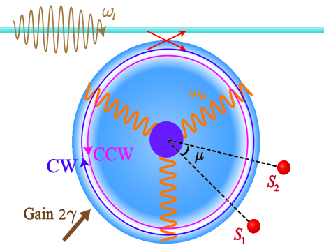
As depicted in Fig. 1, we consider a WGM resonator consisting of two optical modes, where the coupling between two modes is nonreciprocal, which can be achieved by two nanoparticles Zhu1823535 . This resonator driven by a laser with the frequency also supports a phonon mode at the mechanical frequency . Two silica nanotips as Rayleigh scatterers are placed in the evanescent field of the resonator, which are fabricated by the wet etching of tapered fiber tips prepared by heating and stretching standard optical fibers. The position of each particle is controlled by a nanopositioner, which tunes the relative position and effective size of the nanoparticle in the WGM fields. The non-Hermitian optical coupling of the CW and CCW traveling waves induced by the nanoparticles is described by the scattering rates Wiersig063828 ; Wiersig203901 ; Li1909
| (1) | ||||
where () corresponds to the scattering from the CCW (CW) mode to the CW (CCW) mode. is the azimuthal mode number. denotes the relative angular position of the two scatterers. is the complex frequency splitting induced by the th scatterer, which depends on the volume of the th particle within the WGM fields, and is tuned by controlling the distance between the particle and resonator with nanopositioners. Steering the angle can bring the system to EPs, as already observed experimentally Chen548192 ; Peng1136845 . Moreover, we present some discussions on the experimental implementation of Eq. (1) in Appendix A. In the rotating frame , the total non-Hermitian Hamiltonian of the system is written as ()
| (2) | ||||
where () and () denote the photon annihilation and creation operators of the CW (CCW) mode, respectively, satisfying and . () is the phonon annihilation (creation) operator of the mechanical mode. is the detuning between cavity and laser with , where is the frequency of the bare system. The effective loss rate is reduced by the gain (round-trip energy gain) and intrinsic loss rate () McCall289 ; Armani925 ; Peng394 . In consideration of a small change in the cavity length, the cavity optomechanical coupling coefficient is written as , where is the radius of the resonator, and denotes the effective mass of the mechanical mode. denotes the amplitude of the laser field with power .
With the unitary transformation , Eq. (2) becomes
| (3) | ||||
where we made the weak optomechanical coupling approximation, i.e., . The derivation details of Eq. (3) can be found in Appendix B. We find that the mechanical mode is decoupled with the optical cavity, which means the evolutions of optical and mechanical parts are independent of each other, i.e., the state evolution of the total system . When we study the photon statistical properties in the system, the mechanical part in Eq. (3) can be ignored safely, and then Eq. (3) becomes
| (4) | ||||
where denotes the Kerr-type nonlinear strength induced by the optomechanical coupling. We also discuss the equivalence between the original Hamiltonian (2) and effective Hamiltonian (4) under the weak optomechanical coupling approximation in Appendix C, which shows that the used approximation is valid.
The effective Hamiltonian (4) without the effective loss rate can be partitioned into Hermitian and anti-Hermitian parts: , where we have and . To correctly account for the driven-dissipative character of the system, we introduce the Lindblad master equation for the system density matrix
| (5) | ||||
where denotes the Lindblad superoperator term for the annihilation operator acting on the density matrix to account for losses to the environment. is defined as . and denote the effective damping constants of CW and CCW modes, respectively. Without loss of generality, we assume that the decay rates and eigenfrequencies of the resonator modes are respectively equal, i.e., , (). The steady-state solution of the density matrix is obtained by setting in Eq. (5).
III Photon statistical properties
In this section, we analyze CPB at EPs in detail and investigate the photon statistical properties with various relative angular positions of two nanoparticles, which are carried out by simulating the quantum master equation numerically. First of all, the photon statistical properties of CW mode are described by the second-order correlation function of the steady state defined by
| (6) |
which emphasizes the joint probability of detecting two photons at the same time. The case of corresponds to photon antibunching (bunching) in the cavity mode, which is a nonclassical effect.
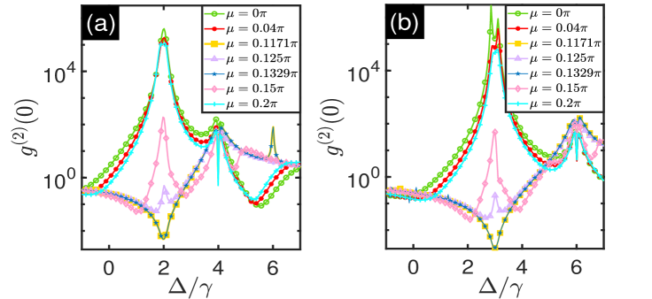
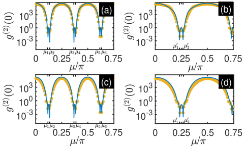
Figure 2 shows as a function of the detuning with various angles , which is solved by Eq. (5). In order to exactly obtain the numerical results about detuning, we assume to be real by choosing proper parameters Peng1136845 ; Vahala839 ; Spillane013817 ; Huet133902 : , , , . In Fig. 2(a), the bunching () is observed at and the maximum bunching is obtained for . Changing to and , the bunching effects are obviously weakened, as shown the purple-triangle line and pink-diamond line in Fig. 2(a). However, at , the most striking feature is the occurrence of PB () when the driving field is in resonance with the cavity, i.e., , as seen the blue-pentagram line and yellow-square line in Fig. 2(a). Moreover, increasing the Kerr-type nonlinear strength to has the similar observation with Fig. 2(a) for , as shown in Fig. 2(b). Appendix D presents the discussion of special points and in Fig. 2(a) and (b).
To gain more insights into CPB shown in Fig. 2, we investigate the eigenenergy of the non-Hermitian Hamiltonian. In the weak driving regime (), the Hilbert space of this system can be restricted in a subspace with few photons spanned by the basis states with the total excitation number , which denotes the Fock state with photons in the bare CW mode and photons in the CCW mode. In the single-excitation subspace, we write the eigenenergies of the non-Hermitian Hamiltonian (4) without the driving term as
| (7) |
with the corresponding non-normalized eigenstates
| (8) |
where . Moreover, we also obtain the eigenenergies and corresponding non-normalized eigenstates , in the two-excitation subspace, where , , and . This shows that the eigenmode structure depending on the asymmetry of the coupling coefficients and can be tuned by controlling the relative angular position between the nanoparticles.
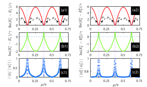
Different from the degeneracy of eigenenergies, EPs correspond to the situation where both two eigenenergies and their eigenstates coalesce Konotop88035002 ; Wiersig033809 . To find EPs of the non-Hermitian system, we plot the real and imaginary parts of the frequency splitting, and the scalar product between the eigenstates associated with the Hamiltonian (4) without the driving field as functions of , as shown in Fig. 3, which manifests has two EPs (e.g., , in Fig. 3) with the energy . In this case, EPs emerge when , which leads to or equalling zero. The case of and corresponds to solely CW propagation, where the eigenstate is composed of only a single Fock state, i.e., , while the case of and is associated with the CCW propagation. From or (resulting in ), we obtain
| (9) |
where corresponds to as shown , , and in Fig. 3, while denotes as seen , , and in Fig. 3.
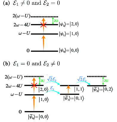
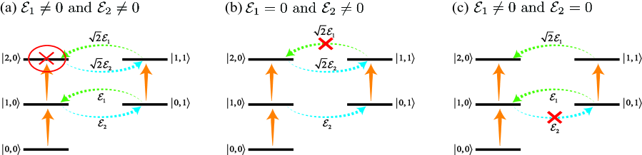
Coincidentally, the special in Fig. 2 happens at EPs and as shown in Fig. 3, where the photon statistical properties become extremely interesting. We first discuss the case of and in Fig. 4(a). In this case, the eigenenergy of the system is with the unique eigenstate in the single-excitation subspace. Furthermore, in the two-excitation subspace, the eigenstate composed of only a Fock state has exact energy . Indeed, the indirect paths , , and are forbidden due to at EPs, which induces predominantly CW propagating mode. Additionally, the direct path to the two-photon state in CW mode is allowed. Note that the uneven spacing of the energy levels is induced by the nonlinearity, which leads to the strong suppression of the absorption of two photons from the incident laser. Therefore, CPB of the CW mode occurs at the EP .
Moreover, a very different situation appears for and in Fig. 4(b), where there is a unique eigenstate consisting of only a single-photon Fock state, whose energy is exactly in the single-excitation subspace. The two-excitation eigenstate formed by only a Fock state has the exact eigenenergy . The indirect paths , , and are blocked due to at EPs. In other words, only the CW mode couples to the CCW mode, while the CCW mode cannot couple to the CW mode for , which suggests CCW propagating mode is predominant. means that the CW excitation induced by the driving field is scattered to the CCW mode, and the same is true for the two-excitation subspace. Additionally, the transition from to is forbidden due to the Kerr-type nonlinearity. Therefore, the probability of the second photon in the CW mode is suppressed, which indicates the presence of EPs results in the occurrence of CPB for the CW mode.
Indeed, for and , the physics is dominated by the photon of CW mode since the eigenstates in the single- and two-excitation subspaces are composed of only a single Fock state of CW mode. For and , CCW photons are populated in the resonator due to the eigenstates consisting of only a Fock state of CCW mode. The reason for this difference is the nonreciprocal coupling between CW and CCW modes at EPs. Nevertheless, we observe effective CPB for the CW mode in two cases, associated with the suppression of the state . In addition, CPB occurs at EPs if the eigenenergy of the single-excitation subspace is exactly equal to the laser frequency, i.e., or (see below Eq. (5)), where the probability of the single-photon state is enhanced. CPB at EPs shows the influence of EPs on the quantum properties of the non-Hermitian system.
IV comprehensive analysis
Under the weak driving condition, the state of the system at any time is expanded as
| (10) |
where represents the probability amplitude of the state , and satisfies . Defining
| (11) | ||||
and substituting Eqs. (4) and (10) into Schrödinger equation, we obtain the steady-state probability amplitude equations
| (12) | ||||
which lead to and
| (13) |
with ignoring higher-order terms in Eq. (12), where and . With these results, we obtain
| (14) |
At EPs (), when the detuning is close to (), the second-order correlation function tends to zero, i.e.,
| (15) |
If the detuning approaches (), but not at EPs (), tends to infinite (), which confirms that the EP is the necessary condition of CPB for this case. Additionally, adjusting the relative angular position to EPs (), if is not close to (equivalently, does not tend to zero), can be reduced to , which may be either greater than one or less than one due to Eq. (11). However, by tuning the parameter to () and keeping , rapidly decreases to , which indicates the strong antibunching effect. Therefore, the condition of CPB occurring at EPs is given by
| (16) |
which is consistent with the physical interpretations in Sec. III, where the second equation of Eq. (16) can be written as calculated by Eq. (11).
Based on above these, we can explain the relevant CPB phenomena in Fig. 2. Although the physical mechanisms in both cases ( or ) are slightly different, the presence of EPs results in the occurrence of PB for the eigenenergy resonance of the single-excitation subspace, and the results of the two cases are almost identical, as shown and in Fig. 2. The physics behind this similarity can be explained from the analytical solution (14), which is symmetric about and . In other words, depends on the product of and more than their individual. At EPs ( or ), equals zero, which leads to the values of being almost the same in both cases.
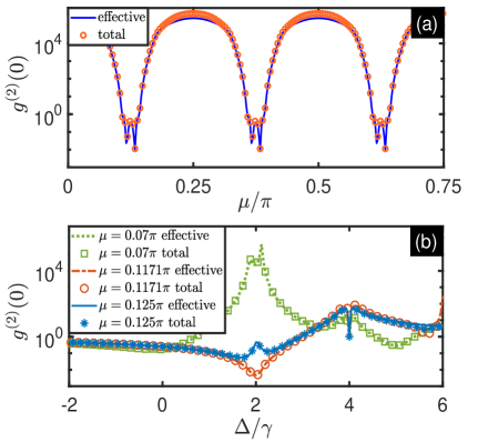
Moreover, we plot the analytical and numerical results for in Fig. 5, and find that the minimum of periodically appears with the increase of , which implies that CPB periodically exists at EPs. In Fig. 5(a) and (b), when the azimuthal mode number is twice as small, the period of the line is twice as large, as also reflected in Fig. 5(c) and (d), which is because determines the period of and in Eq. (1). As seen by Fig. 5(a) and (c), the optimal angle corresponding to CPB occurring remains unchanged as varies, which originates from the fact that does not affect the condition (16) in case of imposing , but it can enhance the performance of PB (also see Fig. 5(b) and (d)). The more photon statistical properties of CPB at EPs can be found in Appendix E.
Before concluding the section, we present a discussion of CPB at non-EPs. Considering that the occurrence of CPB needs to meet the single-excitation eigenenergy resonance, the driven laser frequency (real number) is exactly equal to the eigenenergy in Eq. (7) (i.e., or see below Eq. (5)), which requires the eigenenergies and are real. Therefore, the condition of CPB at non-EPs is given by
| (17) |
which can lead to
| (18) | ||||
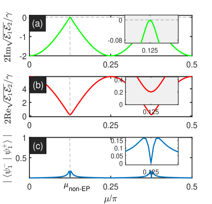
where denotes the argument of the complex number . In order to consider non-EPs (i.e., ), we adjust and (satisfying Eq. (9) at EPs in Sec. III) to and , which meet the requirement for non-EPs given by Eq. (17). Fig. 6(a) shows the imaginary part of the complex eigenenergy splitting equals zero at , which is consistent with that calculated from Eq. (18). In this case, the real part of is not zero (i.e., as shown in the insert of Fig. 6(b)) and the scalar product between the eigenstates tends to zero in Fig. 6(c), which implies that it is a non-EP.
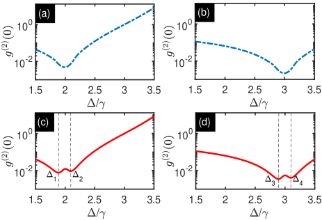
Fig. 7(a) and (b) show versus the detuning at the EP with and , while Fig. 7(c) and (d) correspond to at the non-EP with and . If the laser frequency is exactly equal to the eigenenergy , CPB emerges at the non-EP in Fig. 7(c) as shown and , which are obtained from in Eq. (17) with and given by Fig. 6(b). In this case, we show that the eigenstate in the single-excitation subspace splits from one (coalescence) at EPs to two ( and ) at non-EPs. If , and remain unchanged due to not affecting scattering rates and given by Eq. (1), which results in the occurrence of CPB at the optimal detunings and in Fig. 7(d).
V discussions on UPB
In order to give a complete description of the non-Hermitian system, we discuss UPB at non-EPs and EPs.
(1) UPB can exist at non-EPs (), where the optimal condition can be derived by setting in Eq. (13). Taking the imaginary part of Eq. (13) as zero, we have
| (19) |
while the real part of Eq. (13) equalling zero leads to
| (20) |
which induces (or ) due to . Substituting Eq. (1) into Eq. (19), we have
| (21) |
With Eqs. (21) and (1), Eq. (20) gives
| (22) |
where
with . We notice that when the optimal conditions in Eqs. (21) and (22) simultaneously are satisfied, the strong antibunching can be obtained, otherwise the system is not in the strong antibunching regime.
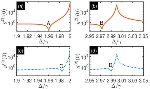
In Fig. 8(a), taking , , , and , UPB occurs at and given by Eqs. (21) and (22), which explain the point A, while and at are given as the point B in Fig. 8(b). Moreover, the point C in Fig. 8(c) corresponds to the optimal conditions and for calculated by Eqs. (21) and (22) when we change to . The point D in Fig. 8(d) is evaluated by and at . The energy levels and transition paths are shown in Fig. 9(a), where the non-zero nonreciprocal scattering rates and lead to the occurrence of the destructive quantum interference between two different excitation paths.
(2) UPB does not exist at EPs, which is discussed as follows.
(i) The destructive quantum interference between two (or more) different excitation paths occurs for the existence of UPB. With Eq. (12), leads to
| (23) | ||||
which corresponds to Fig. 9(b). We note that there is only one path for the system to reach the two-photon state given by Eq. (23) of CW mode, i.e., the direct transition .
For , we have
| (24) | ||||
where the steady-state solution can be obtained. Therefore, the transition to the two-photon state only contains in Fig. 9(c). The destructive quantum interference cannot occur due to Eqs. (23) and (24), which results in UPB not existing.
(ii) UPB requires . At EPs ( or ), the optimal conditions ( and ) given by Eqs. (19) and (20) for UPB existing lead to , which is exactly consistent with Eq. (16) (i.e., the condition of CPB occurring).
In summary, we point out that UPB exists only if the following two conditions are simultaneously satisfied: (I) The destructive quantum interference between two (or more) different excitation paths occurs; (II) The two-photon probability amplitude equals zero. To be specific, the first condition (I) is not met in the case labeled by (i), which leads to the fact that UPB does not exist at EPs.
VI conclusions and discussions
In conclusion, we have found that CPB emerges at EPs of the non-Hermitian optomechanical system coupled with the driven WGM microresonator under the weak optomechanical coupling approximation for the eigenenergy resonance of the single-excitation subspace driven by a laser field. We also discuss the origin of CPB at EPs. For and , with the direct path to the two-photon state in CW mode allowed, CPB emerges due to the anharmonic energy level, where the eigenstates are composed of only a Fock state . For and , the coalescence of eigenstates consisting of only a Fock state causes the system unable to absorb the second photon in the CW mode, which also results in the occurrence of CPB.
Moreover, we study CPB at non-EPs, which occurs for two optimal detunings because of the eigenstate splitting from one (coalescence) at EPs to two at non-EPs in the single-excitation subspace. We also show that UPB does not exist at EPs since the destructive quantum interference cannot occur due to the two different quantum pathways to the two-photon state being not formed, while UPB can occur at non-EPs. In a broader view, our results may have important applications in generating single-photon sources for the non-Hermitian optomechanical system, which aims to improve the performance of quantum sensors Park462 ; Zhang180501 ; Wiersig1 and quantum unidirectional devices Peng1136845 ; Yin175 ; Shen125203 .
ACKNOWLEDGMENTS
This work was supported by National Natural Science Foundation of China under Grants No. 12274064, and Natural Science Foundation of Jilin Province (subject arrangement project) under Grant No. 20210101406JC.
Appendix A Discussions on the experimental implementation
In this section, we present a discussion on the experimental feasibility of observing the prediction for an optomechanical system coupled with the driven WGM microresonator. For the model under study, we mainly focus on the following point: the scatterer-induced nonreciprocal coupling of the CW and CCW traveling lights.
The non-Hermitian optical coupling of the CW and CCW traveling lights can be induced by the nanoparticles, where the isolated microdisk cavity is perturbed by two particles in Refs.Wiersig063828 ; Wiersig203901 . To gain more insights into Eq. (1), we briefly review the two-mode approximation model, whose central assumption is that the small perturbation induced by the nanoparticles couples only the modes within a given degenerate mode pair of the isolated microdisk. The key idea is to model the dynamics in the slowly-varying envelope approximation in the time domain with a Schrödinger-type equation. Considering that the WGM microcavity is an open system, the effective Hamiltonian in the traveling-wave basis (CW, CCW) is given by the non-Hermitian matrix
| (27) |
where the real and imaginary parts of the diagonal element correspond to the frequency of the system and the decay rate of the resonant traveling waves, respectively. The complex-valued off-diagonal element () is the backscattering coefficient, which describes the scattering from the CCW (CW) to the CW (CCW) traveling wave. In general, it is possible that the backscattering between CW and CCW traveling waves is asymmetric, i.e., . For the particular case of the WGM microresonator perturbed through two scatterers, ignoring the frequency shifts for negative-parity modes, the matrix elements of are determined by
| (28) |
where denotes the decay rate. is the azimuthal mode number. is the angular position of scatterer . is the complex frequency splitting induced by scatterer alone. In this case, we take the position of one of the nanoparticles as the reference position. To be specific, we take nanoparticle (see Fig. 1) as the first particle in this model and set its angular position to . Subsequently, the angular position of the second particle is , where denotes the relative angular position of the two nanoparticles. Therefore, the asymmetric backscattering coefficients of CW and CCW traveling waves induced by the nanoparticles are reduced to
| (29) |
which are consistent with Eq. (1). The backscattering coefficients can be adjusted by tuning the relative angle , which modifies the photon statistical properties of the system. It is worth noting that can be calculated for the single-particle-microdisk system either fully numerically (using, e.g., the finite element method Braess , the boundary element method Wiersig553 ) or analytically using the Green’s function approach Dettmann063813 .
Appendix B Derivation of system Hamiltonian
The Hamiltonian of the whole system is given by
| (30) | ||||
where denotes the cavity optomechanics coupling coefficient Grudinin083901 . Making a canonical transformation to the annihilation operator and creation operator as and , Eq. (30) is reduced to
| (31) | ||||
where is the resonance frequency of the th cavity, and the cavity optomechanics coupling coefficient can be changed as . By performing a rotating transformation defined by , Eq. (31) becomes
| (32) | ||||
which corresponds to Eq. (2). In order to decouple the mechanical resonator from the total Hamiltonian, the Hamiltonian (32) with the time-independent unitary transformation by leads to
| (33) | ||||
| . | ||||
With Sakurai2017 , we have the following identities
| (34) | ||||
and then obtain from Eq. (33) as follows
| (35) | ||||
Under the weak optomechanical coupling approximation (), Eq. (3) can be obtained by approximating to in Eq. (35).
Appendix C the validity of approximate hamiltonian
In this model, the crucial factor in investigating the photon statistical properties is whether the effective Hamiltonian (4) is equivalent to the total Hamiltonian (2) in the case of weak optomechanical coupling. To check the validity of effective Hamiltonian in Eq. (4), we give the quantum master equation for the optomechanical system
| (36) | ||||
where and denote the Hermitian and anti-Hermitian parts of the total Hamiltonian given by Eq. (2), respectively.
To further clarify the equivalence between the effective Hamiltonian (4) and total Hamiltonian (2), we compare with steady states of two cases for the fixed detuning . The steady-state density operators are obtained from the numerical solutions of in Eq. (5) and in Eq. (36), respectively. Fig. 10(a) displays as a function of in the case of weak optomechanical coupling, where the numerical result corresponding to effective master equation (5) (blue-solid line) agrees well with that based on the total master equation (36) (red circles). In addition, we also plot as a function of with various angles , as shown in Fig. 10(b), which suggests that the results of the effective master equation (5) and total master equation (36) are consistent for different .
All of these calculations clearly show the equivalence of the optomechanical system given by Eq. (36) and Kerr-type nonlinearity of Eq. (5) in the appropriate parameter regime. It is valid that we use the effective master equation (5) instead of the total master equation (36) to solve this problem. In this case, we can reduce the dimension of the Hilbert space, which makes solving the problem much more accessible.
Appendix D Supplementary discussion of Figure 2
We note that there is a dip in for given by Fig. 2(a) corresponding to the photon bunching, which is revealed from Fig. 11(a), where the dip appears in for due to the fact that the cusp occurs in . Fig. 11(b) has the similar observation at .
Appendix E Supplementary discussion of CPB
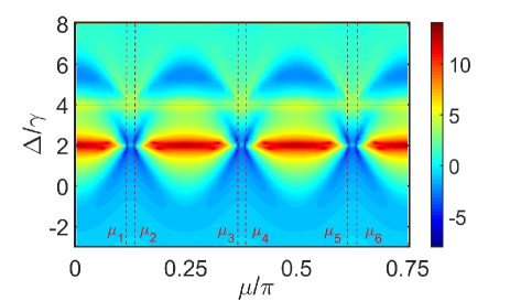
The Appendix gives more discussions on the photon statistical properties of CPB at EPs. We first plot of the CW mode in a logarithmic scale as a function of and , as shown in Fig. 12. changes periodically with the increase of , which originates from the period of coupling coefficients and given by Eq. (1). It is worth noting that there are local minimum values of at the EP when is equal to , i.e., , as shown the intersections of horizontal () and vertical () coordinates in Fig. 12, which agrees well with the results in Fig. 2(a). However, if we adjust the relative angular position away from EPs (e.g., ), arrives at the maximum for .
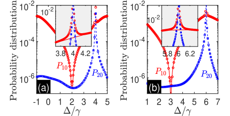
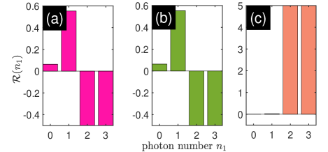
Moreover, CPB at EPs can also be confirmed by comparing the photon-number distribution with the standard Poisson distribution . Therefore, we investigate the relative photon distributions of CW mode , as shown in Fig. 13. When we adjust to EPs ( in Fig. 13(a) and in Fig. 13(b)), the photon-number distribution is greater than the standard Poisson distribution for the single-excitation subspace (), i.e., . However, if the photon number is greater than or equal to , the photon-number distribution is less than the standard Poisson distribution , i.e., . It suggests that the photon is more inclined to exist singly, namely the sub-Poisson distribution, which is the antibunching effect. This confirms CPB at EPs from another aspect. If we tune away from EPs, e.g., in Fig. 13(c), the phenomenon is strikingly different, which indicates the bunching effect. In summary, Fig. 13 shows that is enhanced while is suppressed at EPs, which is in sharp contrast to the case where we change the relative angular position away from EPs.
References
- (1) A. Imamoǧlu, H. Schmidt, G. Woods, and M. Deutsch, Strongly Interacting Photons in a Nonlinear Cavity, Phys. Rev. Lett. 79, 1467 (1997).
- (2) K. M. Gheri, W. Alge, and P. Grangier, Quantum analysis of the photonic blockade mechanism, Phys. Rev. A 60, R2673 (1999).
- (3) A. D. Greentree, J. A. Vaccaro, S. R. de Echaniz, A. V. Durrant, and J. P. Marangos, Prospects for photon blockade in four-level systems in the N configuration with more than one atom, J. Opt. B: Quantum Semiclassical Opt. 2, 252 (2000).
- (4) S. Rebić, A. S. Parkins, and S. M. Tan, Photon statistics of a single-atom intracavity system involving electromagnetically induced transparency, Phys. Rev. A 65, 063804 (2002).
- (5) O. Kyriienko and T. C. H. Liew, Triggered single-photon emitters based on stimulated parametric scattering in weakly nonlinear systems, Phys. Rev. A 90, 063805 (2014).
- (6) S. Ferretti, L. C. Andreani, H. E. Türeci, and D. Gerace, Photon correlations in a two-site nonlinear cavity system under coherent drive and dissipation, Phys. Rev. A 82, 013841 (2010).
- (7) S. Ferretti, V. Savona, and D. Gerace, Optimal antibunching in passive photonic devices based on coupled nonlinear resonators, New J. Phys. 15, 025012 (2013).
- (8) M. Bamba and C. Ciuti, Counter-polarized single-photon generation from the auxiliary cavity of a weakly nonlinear photonic molecule, Appl. Phys. Lett. 99, 171111 (2011).
- (9) S. Ferretti and D. Gerace, Single-photon nonlinear optics with Kerr-type nanostructured materials, Phys. Rev. B 85, 033303 (2012).
- (10) M. Bajcsy, A. Majumdar, A. Rundquist, and J. Vučković, Photon blockade with a four-level quantum emitter coupled to a photonic-crystal nanocavity, New J. Phys. 15, 025014 (2013).
- (11) I. Carusotto and C. Ciuti, Quantum fluids of light, Rev. Mod. Phys. 85, 299 (2013).
- (12) A. Majumdar and D. Gerace, Single-photon blockade in doubly resonant nanocavities with second-order nonlinearity, Phys. Rev. B 87, 235319 (2013).
- (13) A. Majumdar, C. M. Dodson, T. K. Fryett, A. Zhan, S. Buckley, and D. Gerace, Hybrid 2D material nanophotonics: A scalable platform for low-power nonlinear and quantum optics, ACS Photonics 2, 1160 (2015).
- (14) H. Flayac and V. Savona, Input-output theory of the unconventional photon blockade, Phys. Rev. A 88, 033836 (2013).
- (15) D. Gerace and V. Savona, Unconventional photon blockade in doubly resonant microcavities with second-order nonlinearity, Phys. Rev. A 89, 031803(R) (2014).
- (16) Y. H. Zhou, H. Z. Shen, and X. X. Yi, Unconventional photon blockade with second-order nonlinearity, Phys. Rev. A 92, 023838 (2015).
- (17) J. H. Li, R. Yu, and Y. Wu, Proposal for enhanced photon blockade in parity-time-symmetric coupled microcavities, Phys. Rev. A 92, 053837 (2015).
- (18) V. Giovannetti, S. Lloyd, and L. Maccone, Advances in quantum metrology, Nat. Photonics 5, 222 (2011).
- (19) E. Knill, R. Laflamme, and G. J. Milburn, A scheme for efficient quantum computation with linear optics, Nature (London) 409, 46 (2001).
- (20) P. Kok, W. J. Munro, K. Nemoto, T. C. Ralph, J. P. Dowling, and G. J. Milburn, Linear optical quantum computing with photonic qubits, Rev. Mod. Phys. 79, 135 (2007).
- (21) K. Wang, Q. Wu, Y. F. Yu, and Z. M. Zhang, Nonreciprocal photon blockade in a two-mode cavity with a second-order nonlinearity, Phys. Rev. A 100, 053832 (2019).
- (22) S. T. Shen, J. H. Li, and Y. Wu, Magnetically controllable photon blockade under a weak quantum-dot-cavity coupling condition, Phys. Rev. A 101, 023805 (2020).
- (23) D. Stefanatos and E. Paspalakis, Dynamical blockade in a bosonic Josephson junction using optimal coupling, Phys. Rev. A 102, 013716 (2020).
- (24) Y. Ren, S. H. Duan, W. Z. Xie, Y. K. Shao, and Z. L. Duan, Antibunched photon-pair source based on photon blockade in a nondegenerate optical parametric oscillator, Phys. Rev. A 103, 053710 (2021).
- (25) T. C. H. Liew and V. Savona, Single Photons from Coupled Quantum Modes, Phys. Rev. Lett. 104, 183601 (2010).
- (26) M. Bamba, A. Imamoǧlu, I. Carusotto, and C. Ciuti, Origin of strong photon antibunching in weakly nonlinear photonic molecules, Phys. Rev. A 83, 021802(R) (2011).
- (27) H. Flayac and V. Savona, Unconventional photon blockade, Phys. Rev. A 96, 053810 (2017).
- (28) H. J. Carmichael, Photon Antibunching and Squeezing for a Single Atom in a Resonant Cavity, Phys. Rev. Lett. 55, 2790 (1985).
- (29) E. Z. Casalengua, J. C. L. Carreño, F. P. Laussy, and E. del Valle, Conventional and unconventional photon statistics, Laser Photonics Rev. 14, 1900279 (2020).
- (30) O. Kyriienko, I. A. Shelykh, and T. C. H. Liew, Tunable single-photon emission from dipolaritons, Phys. Rev. A 90, 033807 (2014).
- (31) X. W. Xu and Y. Li, Tunable photon statistics in weakly nonlinear photonic molecules, Phys. Rev. A 90, 043822 (2014).
- (32) X. W. Xu and Y. Li, Strongly correlated two-photon transport in a one-dimensional waveguide coupled to a weakly nonlinear cavity, Phys. Rev. A 90, 033832 (2014).
- (33) X. W. Xu and Y. Li, Strong photon antibunching of symmetric and antisymmetric modes in weakly nonlinear photonic molecules, Phys. Rev. A 90, 033809 (2014).
- (34) W. Zhang, Z. Y. Yu, Y. M. Liu, and Y. W. Peng, Optimal photon antibunching in a quantum-dot-bimodal-cavity system, Phys. Rev. A 89, 043832 (2014).
- (35) J. Tang, W. D. Geng, and X. L. Xu, Quantum interference induced photon blockade in a coupled single quantum dot-cavity system, Sci. Rep. 5, 9252 (2015).
- (36) X. Y. Liang, Z. L. Duan, Q. Guo, S. G. Guan, M. Xie, and C. J. Liu, Photon blockade in a bimode nonlinear nanocavity embedded with a quantum dot, Phys. Rev. A 102, 053713 (2020).
- (37) J. Wang, Q. Wang, and H. Z. Shen, Nonreciprocal unconventional photon blockade with spinning atom-cavity, Europhys. Lett. 134, 64003 (2021).
- (38) D. Roberts and A. A. Clerk, Driven-Dissipative Quantum Kerr Resonators: New Exact Solutions, Photon Blockade and Quantum Bistability, Phys. Rev. X 10, 021022 (2020).
- (39) H. Flayac and V. Savona, Single photons from dissipation in coupled cavities, Phys. Rev. A 94, 013815 (2016).
- (40) H. Flayac, D. Gerace, and V. Savona, An all-silicon single-photon source by unconventional photon blockade, Sci. Rep. 5, 11223 (2015).
- (41) H. Z. Shen, Y. H. Zhou, H. D. Liu, G. C. Wang, and X. X. Yi, Exact optimal control of photon blockade with weakly nonlinear coupled cavities, Opt. Express 23, 32835 (2015).
- (42) H. Z. Shen, S. Xu, Y. H. Zhou, G. C. Wang, and X. X. Yi, Unconventional photon blockade from bimodal driving and dissipations in coupled semiconductor microcavities, J. Phys. B: At. Mol. Opt. Phys. 51, 035503 (2018).
- (43) Y. H. Zhou, H. Z. Shen, X. Q. Shao, and X. X. Yi, Strong photon antibunching with weak second-order nonlinearity under dissipation and coherent driving, Opt. Express 24, 17332 (2016).
- (44) F. Zou, D. G. Lai, and J. Q. Liao, Enhancement of photon blockade effect via quantum interference, Opt. Express 28, 16175 (2020).
- (45) V. Savona, Unconventional photon blockade in coupled optomechanical systems, arXiv:1302.5937 (2013).
- (46) K. Hou, C. J. Zhu, Y. P. Yang, and G. S. Agarwal, Interfering pathways for photon blockade in cavity QED with one and two qubits, Phys. Rev. A 100, 063817 (2019).
- (47) X. W. Xu and Y. J. Li, Antibunching photons in a cavity coupled to an optomechanical system, J. Phys. B: At. Mol. Opt. Phys. 46, 035502 (2013).
- (48) Y. Qu, J. H. Li, and Y. Wu, Interference-modulated photon statistics in whispering-gallery-mode microresonator optomechanics, Phys. Rev. A 99, 043823 (2019).
- (49) Y. H. Zhou, H. Z. Shen, X. Y. Zhang, and X. X. Yi, Zero eigenvalues of a photon blockade induced by a non-Hermitian Hamiltonian with a gain cavity, Phys. Rev. A 97, 043819 (2018).
- (50) J. C. López Carreño, C. Sánchez Muñoz, D. Sanvitto, E. del Valle, and F. P. Laussy, Exciting polaritons with quantum light, Phys. Rev. Lett. 115, 196402 (2015).
- (51) H. Z. Shen, C. Shang, Y. H. Zhou, and X. X. Yi, Unconventional single-photon blockade in non-Markovian systems, Phys. Rev. A 98, 023856 (2018).
- (52) H. Z. Shen, Q. Wang, J. Wang, and X. X. Yi, Nonreciprocal unconventional photon blockade in a driven dissipative cavity with parametric amplification, Phys. Rev. A 101, 013826 (2020).
- (53) B. Sarma and A. K. Sarma, Quantum-interference-assisted photon blockade in a cavity via parametric interactions, Phys. Rev. A 96, 053827 (2017).
- (54) M. A. Lemonde, N. Didier, and A. A. Clerk, Antibunching and unconventional photon blockade with Gaussian squeezed states, Phys. Rev. A 90, 063824 (2014).
- (55) K. M. Birnbaum, A. Boca, R. Miller, A. D. Boozer, T. E. Northup, and H. J. Kimble, Photon blockade in an optical cavity with one trapped atom, Nature (London) 436, 87 (2005)
- (56) H. Z. Shen, Y. H. Zhou, and X. X. Yi, Quantum optical diode with semiconductor microcavities, Phys. Rev. A 90, 023849 (2014).
- (57) T. E. Lee and M. C. Cross, Quantum-classical transition of correlations of two coupled cavities, Phys. Rev. A 88, 013834 (2013).
- (58) Y. H. Zhou, X. Y. Zhang, Q. C. Wu, B. L. Ye, Z. Q. Zhang, D. D. Zou, H. Z. Shen, and C. P. Yang, Conventional photon blockade with a three-wave mixing, Phys. Rev. A 102, 033713 (2020).
- (59) R. Huang, A. Miranowicz, J. Q. Liao, F. Nori, and H. Jing, Nonreciprocal Photon Blockade, Phys. Rev. Lett. 121, 153601 (2018).
- (60) J. Kim, O. Benson, H. Kan, and Y. Yamamoto, A single-photon turnstile device, Nature 397, 500 (1999).
- (61) I. I. Smolyaninov, A. V. Zayats, A. Gungor, and C. C. Davis, Single-photon tunneling via localized surface plasmons, Phys. Rev. Lett. 88, 187402 (2002).
- (62) H. X. Zheng, D. J. Gauthier, and H. U. Baranger, Cavity-Free Photon Blockade Induced by Many-Body Bound States, Phys. Rev. Lett. 107, 223601 (2011).
- (63) A. Majumdar, M. Bajcsy, A. Rundquist, and J. Vučković, Loss-enabled sub-Poissonian light generation in a bimodal nanocavity, Phys. Rev. Lett. 108, 183601 (2012).
- (64) M. Hennrich, A. Kuhn, and G. Rempe, Transition from Antibunching to Bunching in Cavity QED, Phys. Rev. Lett. 94, 053604 (2005).
- (65) C. Hamsen, K. N. Tolazzi, T. Wilk, and G. Rempe, Two-Photon Blockade in an Atom-Driven Cavity QED System, Phys. Rev. Lett. 118, 133604 (2017).
- (66) A. Ridolfo, M. Leib, S. Savasta, and M. J. Hartmann, Photon Blockade in the Ultrastrong Coupling Regime, Phys. Rev. Lett. 109, 193602 (2012).
- (67) L. Tian and H. J. Carmichael, Quantum trajectory simulations of two-state behavior in an optical cavity containing one atom, Phys. Rev. A 46, R6801(R) (1992).
- (68) M. J. Werner and A. Imamoḡlu, Photon-photon interactions in cavity electromagnetically induced transparency, Phys. Rev. A 61, 011801(R) (1999).
- (69) R. J. Brecha, P. R. Rice, and M. Xiao, N two-level atoms in a driven optical cavity: Quantum dynamics of forward photon scattering for weak incident fields, Phys. Rev. A 59, 2392 (1999).
- (70) S. Rebić, S. M. Tan, A. S. Parkins, and D. F. Walls, Large Kerr nonlinearity with a single atom, J. Opt. B: Quantum Semiclassical Opt. 1, 490 (1999).
- (71) X. Y. Liang, Z. L. Duan, Q. Guo, C. J. Liu, S. G. Guan, and Y. Ren, Antibunching effect of photons in a two-level emitter-cavity system, Phys. Rev. A 100, 063834 (2019).
- (72) Y. Y. Yan, Y. B. Cheng, S. G. Guan, D. Y. Yu, and Z. L. Duan, Pulse-regulated single-photon generation via quantum interference in a nonlinear nanocavity, Opt. Lett. 43, 5086 (2018).
- (73) J. M. Fink, A. Dombi, A. Vukics, A. Wallraff, and P. Domokos, Observation of the Photon-Blockade Breakdown Phase Transition, Phys. Rev. X 7, 011012 (2017).
- (74) J. Q. Liao and C. K. Law, Correlated two-photon transport in a one-dimensional waveguide side-coupled to a nonlinear cavity, Phys. Rev. A 82, 053836 (2010).
- (75) A. Miranowicz, M. Paprzycka, Y. X. Liu, J. Bajer, and F. Nori, Two-photon and three-photon blockades in driven nonlinear systems, Phys. Rev. A 87, 023809 (2013).
- (76) C. J. Zhu, Y. P. Yang, and G. S. Agarwal, Collective multiphoton blockade in cavity quantum electrodynamics, Phys. Rev. A 95, 063842 (2017).
- (77) J. Z. Lin, K. Hou, C. J. Zhu, and Y. P. Yang, Manipulation and improvement of multiphoton blockade in a cavity-QED system with two cascade three-level atoms, Phys. Rev. A 99, 053850 (2019).
- (78) A. Faraon, A. Majumdar, and J. Vučković, Generation of nonclassical states of light via photon blockade in optical nanocavities, Phys. Rev. A 81, 033838 (2010).
- (79) C. Lang, D. Bozyigit, C. Eichler, L. Steffen, J. M. Fink, A. A. Abdumalikov, Jr., M. Baur, S. Filipp, M. P. da Silva, A. Blais, and A. Wallraff, Observation of Resonant Photon Blockade at Microwave Frequencies Using Correlation Function Measurements, Phys. Rev. Lett. 106, 243601 (2011).
- (80) Y. X. Liu, X. W. Xu, A. Miranowicz, and F. Nori, From blockade to transparency: Controllable photon transmission through a circuit-QED system, Phys. Rev. A 89, 043818 (2014).
- (81) M. Leib and M. J. Hartmann, Bose-Hubbard dynamics of polaritons in a chain of circuit quantum electrodynamics cavities, New J. Phys. 12, 093031 (2010).
- (82) A. J. Hoffman, S. J. Srinivasan, S. Schmidt, L. Spietz, J. Aumentado, H. E. Türeci, and A. A. Houck, Dispersive Photon Blockade in a Superconducting Circuit, Phys. Rev. Lett. 107, 053602 (2011).
- (83) P. Rabl, Photon Blockade Effect in Optomechanical Systems, Phys. Rev. Lett. 107, 063601 (2011).
- (84) H. Wang, X. Gu, Y. X. Liu, A. Miranowicz, and F. Nori, Tunable photon blockade in a hybrid system consisting of an optomechanical device coupled to a two-level system, Phys. Rev. A 92, 033806 (2015).
- (85) A. Nunnenkamp, K. Børkje, and S. M. Girvin, Single-photon optomechanics, Phys. Rev. Lett. 107, 063602 (2011).
- (86) C. L. Zhai, R. Huang, H. Jing, and L. M. Kuang, Mechanical switch of photon blockade and photon-induced tunneling, Opt. Express 27, 27649 (2019).
- (87) J. Q. Liao and F. Nori, Photon blockade in quadratically coupled optomechanical systems, Phys. Rev. A 88, 023853 (2013).
- (88) P. Kómár, S. D. Bennett, K. Stannigel, S. J. M. Habraken, P. Rabl, P. Zoller, and M. D. Lukin, Single-photon nonlinearities in two-mode optomechanics, Phys. Rev. A 87, 013839 (2013).
- (89) X. Y. Lü, W. M. Zhang, S. Ashhab, Y. Wu, and F. Nori, Quantum-criticality-induced strong Kerr nonlinearities in optomechanical systems, Sci. Rep. 3, 2943 (2013).
- (90) X. N. Xu, M. Gullans, and J. M. Taylor, Quantum nonlinear optics near optomechanical instabilities, Phys. Rev. A 91, 013818 (2015).
- (91) A. Miranowicz, J. Bajer, N. Lambert, Y. X. Liu, and F. Nori, Tunable multiphonon blockade in coupled nanomechanical resonators, Phys. Rev. A 93, 013808 (2016).
- (92) H. Xie, G. W. Lin, X. Chen, Z. H. Chen, and X. M. Lin, Single-photon nonlinearities in a strongly driven optomechanical system with quadratic coupling, Phys. Rev. A 93, 063860 (2016).
- (93) H. Xie, C. G. Liao, X. Shang, M. Y. Ye, and X. M. Lin, Phonon blockade in a quadratically coupled optomechanical system. Phys. Rev. A 96, 013861 (2017).
- (94) F. Zou, L. B. Fan, J. F. Huang, and J. Q. Liao, Enhancement of few-photon optomechanical effects with cross-Kerr nonlinearity, Phys. Rev. A 99, 043837 (2019).
- (95) Y. X. Liu, A. Miranowicz, Y. B. Gao, J. Bajer, C. P. Sun, and F. Nori, Qubit-induced phonon blockade as a signature of quantum behavior in nanomechanical resonators, Phys. Rev. A 82, 032101 (2010).
- (96) D. G. Angelakis, M. F. Santos, and S. Bose, Photon-blockade-induced Mott transitions and XY spin models in coupled cavity arrays, Phys. Rev. A 76, 031805(R) (2007).
- (97) H. Z. Shen, Y. H. Zhou, and X. X. Yi, Tunable photon blockade in coupled semiconductor cavities, Phys. Rev. A 91, 063808 (2015).
- (98) T. Grujic, S. R. Clark, D. Jaksch, and D. G. Angelakis, Non-equilibrium many-body effects in driven nonlinear resonator arrays, New J. Phys. 14, 103025 (2012).
- (99) M. Radulaski, K. A. Fischer, K. G. Lagoudakis, J. L. Zhang, and J. Vučković, Photon blockade in two-emitter-cavity systems, Phys. Rev. A 96, 011801(R) (2017).
- (100) A. L. Boité, M. J. Hwang, H. Nha, and M. B. Plenio, Fate of photon blockade in the deep strong-coupling regime, Phys. Rev. A 94, 033827 (2016).
- (101) Z. G. Li, X. M. Li, and X. L. Zhong, Strong photon blockade in an all-fiber emitter-cavity quantum electrodynamics system, Phys. Rev. A 103, 043724 (2021).
- (102) W. S. Xue, H. Z. Shen, and X. X. Yi, Nonreciprocal conventional photon blockade in driven dissipative atom-cavity, Opt. Lett. 45, 4424 (2020).
- (103) Y. W. Jing, H. Q. Shi, and X. W. Xu, Nonreciprocal photon blockade and directional amplification in a spinning resonator coupled to a two-level atom, Phys. Rev. A. 104, 033707 (2021).
- (104) X. Y. Yao, H. Ali, F. L. Li, and P. B. Li, Nonreciprocal phonon blockade in a spinning acoustic ring cavity coupled to a two-level system, Phys. Rev. Appl. 17, 054004 (2022).
- (105) S. Ghosh and T. C. H. Liew, Dynamical Blockade in a Single-Mode Bosonic System, Phys. Rev. Lett. 123, 013602 (2019).
- (106) A. Faraon, I. Fushman, D. Englund, N. Stoltz, P. Petroff, and J. Vučković, Coherent generation of non-classical light on a chip via photon-induced tunnelling and blockade, Nat. Phys. 4, 859 (2008).
- (107) A. P. Foster, D. Hallett, I. V. Iorsh, S. J. Sheldon, M. R. Godsland, B. Royall, E. Clarke, I. A. Shelykh, A. M. Fox, M. S. Skolnick, I. E. Itskevich, and L. R. Wilson, Tunable Photon Statistics Exploiting the Fano Effect in a Waveguide, Phys. Rev. Lett. 122, 173603 (2019).
- (108) C. Vaneph, A. Morvan, G. Aiello, M. Féchant, M. Aprili, J. Gabelli, and J. Estève, Observation of the Unconventional Photon Blockade in the Microwave Domain, Phys. Rev. Lett. 121, 043602 (2018).
- (109) H. J. Snijders, J. A. Frey, J. Norman, H. Flayac, V. Savona, A. C. Gossard, J. E. Bowers, M. P. van Exter, D. Bouwmeester, and W. Löffler, Observation of the Unconventional Photon Blockade, Phys. Rev. Lett. 121, 043601 (2018).
- (110) R. Loudon, The Quantum Theory of Light (Oxford Science, Oxford, 2000).
- (111) D. Gerace, H. E. Türeci, A. Imamoglu, V. Giovannetti, and R. Fazio, The quantum-optical Josephson interferometer, Nat. Phys. 5, 281 (2009).
- (112) F. Fratini, E. Mascarenhas, L. Safari, J-Ph. Poizat, D. Valente, A. Auffèves, D. Gerace, and M. F. Santos, Fabry-Perot interferometer with quantum mirrors: nonlinear light transport and rectification, Phys. Rev. Lett. 113, 243601 (2014).
- (113) E. Mascarenhas, D. Gerace, D. Valente, S. Montangero, A. Auffèves, and M. F. Santos, A quantum optical valve in a nonlinear-linear resonators junction, Europhys. Lett. 106, 54003 (2014).
- (114) D. E. Chang, A. S. Sørensen, E. A. Demler, and M. D. Lukin, A single-photon transistor using nanoscale surface plasmons, Nat. Phys. 3, 807 (2007).
- (115) T. Ramos, V. Sudhir, K. Stannigel, P. Zoller, and T. J. Kippenberg, Nonlinear Quantum Optomechanics via Individual Intrinsic Two-Level Defects, Phys. Rev. Lett. 110, 193602 (2013).
- (116) D. Y. Wang, C. H. Bai, S. Liu, S. Zhang, and H. F. Wang, Photon blockade in a double-cavity optomechanical system with nonreciprocal coupling. New J. Phys. 22, 093006 (2020).
- (117) X. W. Xu, Y. J. Zhao, H. Wang, H. Jing, and A. X. Chen, Quantum nonreciprocality in quadratic optomechanics, Photon. Res. 8, 143 (2020).
- (118) S. Manipatruni, J. T. Robinson, and M. Lipson, Optical Nonreciprocity in Optomechanical Structures, Phys. Rev. Lett. 102, 213903 (2009).
- (119) Z. Shen, Y. L. Zhang, Y. Chen, C. L. Zou, Y. F. Xiao, X. B. Zou, F. W. Sun, G. C. Guo, and C. H. Dong, Experimental realization of optomechanically induced non-reciprocity, Nat. Photonics 10, 657 (2016).
- (120) N. R. Bernier, L. D. Tóth, A. Koottandavida, M. A. Ioannou, D. Malz, A. Nunnenkamp, A. K. Feofanov, and T. J. Kippenberg, Nonreciprocal reconfigurable microwave optomechanical circuit, Nat. Commun. 8, 604 (2017).
- (121) Y. Jiang, S. Maayani, T. Carmon, F. Nori, and H. Jing, Nonreciprocal Phonon Laser, Phys. Rev. Appl. 10, 064037 (2018).
- (122) B. J. Li, R. Huang, X. W. Xu, A. Miranowicz, and H. Jing, Nonreciprocal unconventional photon blockade in a spinning optomechanical system, Photon. Res. 7, 630 (2019).
- (123) J. H. Liu, Y. F. Yu, and Z. M. Zhang, Nonreciprocal transmission and fast-slow light effects in a cavity optomechanical system, Opt. Express 27, 15382 (2019).
- (124) I. M. Mirza, W. C. Ge, and H. Jing, Optical nonreciprocity and slow light in coupled spinning optomechanical resonators, Opt. Express 27, 25515 (2019).
- (125) Y. F. Jiao, S. D. Zhang, Y. L. Zhang, A. Miranowicz, L. M. Kuang, and H. Jing, Nonreciprocal Optomechanical Entanglement Against Backscattering Losses, Phys. Rev. Lett. 125, 143605 (2020).
- (126) X. Shang, H. Xie, and X. M. Lin, Nonreciprocal photon blockade in a spinning optomechanical resonator, Laser Phys. Lett. 18, 115202 (2021).
- (127) Y. P. Gao and C. Wang, Hybrid coupling optomechanical assisted nonreciprocal photon blockade, Opt. Express 29, 25161 (2021).
- (128) X. W. Xu and Y. Li, Optical nonreciprocity and optomechanical circulator in three-mode optomechanical systems, Phys. Rev. A 91, 053854 (2015).
- (129) G. S. Agarwal and S. Huang, Electromagnetically induced transparency in mechanical effects of light, Phys. Rev. A 81, 041803(R) (2010).
- (130) J. D. Teufel, D. Li, M. S. Allman, K. Cicak, A. J. Sirois, J. D. Whittaker, and R. W. Simmonds, Circuit cavity electromechanics in the strong coupling regime, Nature (London) 471, 204 (2011).
- (131) H. Zhang, F. Saif, Y. Jiao, and H. Jing, Loss-induced transparency in optomechanics, Opt. Express 26, 025199 (2018).
- (132) S. Aldana, C. Bruder, and A. Nunnenkamp, Equivalence between an optomechanical system and a Kerr medium, Phys. Rev. A 88, 043826 (2013).
- (133) L. Zhou, J. Cheng, Y. Han, and W. P. Zhang, Nonlinearity enhancement in optomechanical systems, Phys. Rev. A 88, 063854 (2013).
- (134) X. Y. Lü, Y. Wu, J. R. Johansson, H. Jing, J. Zhang, and F. Nori, Squeezed optomechanics with phase-matched amplification and dissipation, Phys. Rev. Lett. 114, 093602 (2015).
- (135) J. D. Teufel, T. Donner, D. Li, J. W. Harlow, M. S. Allman, K. Cicak, A. J. Sirois, J. D. Whittaker, K. W. Lehnert, and R. W. Simmonds, Sideband cooling of micromechanical motion to the quantum ground state, Nature (London) 475, 359 (2011).
- (136) J. Chan, T. P. M. Alegre, A. H. Safavi-Naeini, J. T. Hill, A. Krause, S. Gröblacher, M. Aspelmeyer, and O. Painter, Laser cooling of a nanomechanical oscillator into its quantum ground state, Nature (London) 478, 89 (2011).
- (137) B. Abbott et al., Observation of a kilogram-scale oscillator near its quantum ground state, New J. Phys. 11, 073032 (2009).
- (138) A. Pontin, M. Bonaldi, A. Borrielli, F. S. Cataliotti, F. Marino, G. A. Prodi, E. Serra, and F. Marin, Detection of weak stochastic forces in a parametrically stabilized micro-optomechanical system, Phys. Rev. A 89, 023848 (2014).
- (139) M. Aspelmeyer, T. J. Kippenberg, and F. Marquardt, Cavity optomechanics, Rev. Mod. Phys. 86, 1391 (2014).
- (140) F. Brennecke, S. Ritter, T. Donner, and T. Esslinger, Cavity Optomechanics with a Bose-Einstein Condensate, Science 322, 235 (2008).
- (141) S. Gupta, K. L. Moore, K. W. Murch, and D. M. Stamper-Kurn, Cavity Nonlinear Optics at Low Photon Numbers from Collective Atomic Motion, Phys. Rev. Lett. 99, 213601 (2007).
- (142) A. Sergi and K. G. Zloshchastiev, Non-Hermitian quantum dynamics of a two-level system and models of dissipative environments, Int. J. Mod. Phys. B 27, 1350163 (2013).
- (143) K. G. Zloshchastiev and A. Sergi, Comparison and unification of non-Hermitian and Lindblad approaches with applications to open quantum optical systems, J. Mod. Opt. 61, 1298 (2014).
- (144) A. Sergi and K. G. Zloshchastiev, Time correlation functions for non-Hermitian quantum systems, Phys. Rev. A 91, 062108 (2015).
- (145) C. M. Bender and S. Boettcher, Real Spectra in NonHermitian Hamiltonians Having PT Symmetry, Phys. Rev. Lett. 80, 5243 (1998).
- (146) C. M. Bender, Making sense of non-Hermitian Hamiltonians, Rep. Prog. Phys. 70, 947 (2007).
- (147) V. V. Konotop, J. Yang, and D. A. Zezyulin, Nonlinear waves in PT-symmetric systems, Rev. Mod. Phys. 88, 035002 (2016).
- (148) L. Feng, R. El-Ganainy, and L. Ge, Non-Hermitian photonics based on parity-time symmetry, Nat. Photonics 11, 752 (2017).
- (149) B. Peng, Ş. K. Özdemir, F. C. Lei, F. Monifi, M. Gianfreda, G. L. Long, S. H. Fan, F. Nori, C. M. Bender, and L. Yang, Parity-time-symmetric whispering-gallery microcavities, Nat. Phys. 10, 394 (2014).
- (150) C. E. Rüter, K. G. Makris, R. El-Ganainy, D. N. Christodoulides, M. Segev, and D. Kip, Observation of parity-time symmetry in optics, Nat. Phys. 6, 192 (2010).
- (151) A. A. Zyablovsky, A. P. Vinogradov, A. A. Pukhov, A. V. Dorofeenko, and A. A. Lisyansky, PT-symmetry in optics, Phys. Usp. 57, 1063 (2014).
- (152) S. Longhi, Parity-time symmetry meets photonics: A new twist in non-Hermitian optics, Europhys. Lett. 120, 64001 (2018).
- (153) H. Lü, C. Wang, L. Yang, and H. Jing, Optomechanically induced transparency at exceptional points, Phys. Rev. Appl. 10, 014006 (2018).
- (154) B. Peng, Ş. K. Özdemir, S. Rotter, H. Yilmaz, M. Liertzer, F. Monifi, C. M. Bender, F. Nori, and L. Yang, Loss-induced suppression and revival of lasing, Science 346, 328 (2014).
- (155) A. Guo, G. J. Salamo, D. Duchesne, R. Morandotti, M. Volatier-Ravat, V. Aimez, G. A. Siviloglou, and D. N. Christodoulides, Observation of PT-Symmetry Breaking in Complex Optical Potentials, Phys. Rev. Lett. 103, 093902 (2009).
- (156) Y. L. Zuo, R. Huang, L. M. Kuang, X. W. Xu, and H. Jing, Loss-induced suppression, revival, and switch of photon blockade, Phys. Rev. A 106, 043715 (2022).
- (157) R. Huang, Şahin. K. Özdemir, J. Q. Liao, F. Minganti, L. M. Kuang, Franco Nori, and H. Jing, Exceptional Photon Blockade: Engineering Photon Blockade with Chiral Exceptional Points, Laser Photonics Rev. 16, 2100430 (2022).
- (158) S. Longhi and L. Feng, Unidirectional lasing in semiconductor microring lasers at an exceptional point, Photonics Res. 5, B1 (2017).
- (159) Z. Lin, H. Ramezani, T. Eichelkraut, T. Kottos, H. Cao, and D. N. Christodoulides, Unidirectional Invisibility Induced by PT-Symmetric Periodic Structures, Phys. Rev. Lett. 106, 213901 (2011).
- (160) S. Assawaworrarit, X. F. Yu, and S. H. Fan, Robust wireless power transfer using a nonlinear parity-time-symmetric circuit, Nature (London) 546, 387 (2017).
- (161) H. Y. Zhou, C. Peng, Y. Yoon, C. W. Hsu, K. A. Nelson, L. Fu, J. D. Joannopoulos, M. Soljačić, and B. Zhen, Observation of bulk Fermi arc and polarization half charge from paired exceptional points, Science 359, 1009 (2018).
- (162) B. Yang, Q. H. Guo, B. Tremain, R. J. Liu, L. E. Barr, Q. H. Yan, W. L. Gao, H. C. Liu, Y. J. Xiang, J. Chen, C. Fang, A. Hibbins, L. Lu, S. Zhang, Ideal Weyl points and helicoid surface states in artificial photonic crystal structures, Science 359, 1013 (2018).
- (163) H. Xu, D. Mason, L. Y. Jiang, and J. G. E. Harris, Topological energy transfer in an optomechanical system with exceptional points, Nature (London) 537, 80 (2016).
- (164) H. Jing, S. K. Özdemir, X. Y. Lü, J. Zhang, L. Yang, and F. Nori, PT-Symmetric Phonon Laser, Phys. Rev. Lett. 113, 053604 (2014).
- (165) H. Lü, S. K. Özdemir, L. M. Kuang, F. Nori, and H. Jing, Exceptional Points in Random-Defect Phonon Lasers, Phys. Rev. Appl. 8, 044020 (2017).
- (166) H. Jing, Ş. K. Özdemir, H. Lü, and F. Nori, High-order exceptional points in optomechanics, Sci. Rep. 7, 3386 (2017).
- (167) B. Peng, Ş. K. Özdemir, M. Liertzer, W. J. Chen, J. Kramer, H. Yilmaz, J. Wiersig, S. Rotter, and L. Yang, Chiral modes and directional lasing at exceptional points, Proc. Natl. Acad. Sci. USA 113, 6845 (2016).
- (168) Q. T. Cao, H. M. Wang, C. H. Dong, H. Jing, R. S. Liu, X. Chen, L. Ge, Q. H. Gong, and Y. F. Xiao, Experimental Demonstration of Spontaneous Chirality in a Nonlinear Microresonator, Phys. Rev. Lett. 118, 033901 (2017).
- (169) W. J. Chen, Ş. K. Özdemir, G. M. Zhao, J. Wiersig, and L. Yang, Exceptional points enhance sensing in an optical microcavity, Nature (London) 548, 192 (2017).
- (170) T. Tian, Z. H. Wang, and L. J. Song, Rotation sensing in two coupled whispering-gallery-mode resonators with loss and gain, Phys. Rev. A 100, 043810 (2019).
- (171) J. G. Zhu, Ş. K. Özdemir, L. N. He, and L. Yang, Controlled manipulation of mode splitting in an optical microcavity by two Rayleigh scatterers, Opt. Express 18, 23535 (2010).
- (172) J. Wiersig, Structure of whispering-gallery modes in optical microdisks perturbed by nanoparticles, Phys. Rev. A 84, 063828 (2011).
- (173) J. Wiersig, Enhancing the Sensitivity of Frequency and Energy Splitting Detection by Using Exceptional Points: Application to Microcavity Sensors for Single-Particle Detection, Phys. Rev. Lett. 112, 203901 (2014).
- (174) W. A. Li, Tunable photon blockade in a whispering-gallery-mode microresonator coupled with two nanoparticles, arXiv:1909.09919 (2019).
- (175) D. K. Armani, T. J. Kippenberg, S. M. Spillane, K. J. Vahala, Ultra-high-Q toroid microcavity on a chip, Nature 421, 925 (2003).
- (176) S. L. McCall, A. F. J. Levi, R. E. Slusher, S. J. Pearton, and R. A. Logan, Whispering-gallery mode microdisk lasers, Appl. Phys. Lett. 60, 289(1992).
- (177) B. Peng, Ş. K. Özdemir, F. C. Lei, F. Monifi, M. Gianfreda, G. L. Long, S. H. Fan, F. Nori, C. M. Bender, and L. Yang, Parity-time-symmetric whispering-gallery microcavities, Nat. Phys. 10, 394 (2014).
- (178) K. J. Vahala, Optical microcavities, Nature (London) 424, 839 (2003).
- (179) S. M. Spillane, T. J. Kippenberg, K. J. Vahala, K. W. Goh, E. Wilcut, and H. J. Kimble, Ultrahigh-Q toroidal microresonators for cavity quantum electrodynamics, Phys. Rev. A 71, 013817 (2005).
- (180) V. Huet, A. Rasoloniaina, P. Guillemé, P. Rochard, P. Féron, M. Mortier, A. Levenson, K. Bencheikh, A. Yacomotti, and Y. Dumeige, Millisecond photon lifetime in a slow-light microcavity, Phys. Rev. Lett. 116, 133902 (2016).
- (181) J. Wiersig, Sensors operating at exceptional points: General theory, Phys. Rev. A 93, 033809 (2016).
- (182) J. H. Park, A. Ndao, W. Cai, L. Hsu, A. Kodigala, T. Lepetit, Y. H. Lo, and B. Kanté, Symmetry-breaking-induced plasmonic exceptional points and nanoscale sensing, Nat. Phys. 16, 462 (2020).
- (183) J. Wiersig, Prospects and fundamental limits in exceptional point-based sensing, Nat. Commun. 11, 1 (2020).
- (184) M. Z. Zhang, W. Sweeney, C. W. Hsu, L. Yang, A. D. Stone, and L. Jiang, Quantum noise theory of exceptional point amplifying sensors, Phys. Rev. Lett. 123, 180501 (2019).
- (185) X. B. Yin and X. Zhang, Unidirectional light propagation at exceptional points, Nat. Mater. 12, 175 (2013).
- (186) C. Shen, J. F. Li, X. Y. Peng, and S. A. Cummer, Synthetic exceptional points and unidirectional zero reflection in non-Hermitian acoustic systems, Phys. Rev. Mater. 2, 125203 (2018).
- (187) D. Braess, Finite Elemente: Theorie, schnelle Löser und Anwendungen in der Elastizitätstheorie (Springer-Verlag, New York, 2013).
- (188) J. Wiersig, Boundary element method for resonances in dielectric microcavities, J. Opt. A: Pure Appl. Opt. 5, 53 (2003).
- (189) C. P. Dettmann, G. V. Morozov, M. Sieber, and H. Waalkens, Unidirectional emission from circular dielectric microresonators with a point scatterer, Phys. Rev. A 80, 063813 (2009).
- (190) I. S. Grudinin, H. Lee, O. Painter, and K. J. Vahala, Phonon Laser Action in a Tunable Two-Level System, Phys. Rev. Lett. 104, 083901 (2010).
- (191) J. J. Sakurai and J. Napolitano, Modern Quantum Mechanics, 2nd ed. (Cambridge University Press, Cambridge, 2017).