Corrected Correlation Estimates for Meta-Analysis

Abstract

Meta-analysis allows rigorous aggregation of estimates and uncertainty across multiple studies. When a given study reports multiple estimates, such as log odds ratios (ORs) or log relative risks (RRs) across exposure groups, accounting for within-study correlations improves accuracy and efficiency of meta-analytic results. Canonical approaches of Greenland-Longnecker [6] and Hamling [8] estimate pseudo cases and non-cases for exposure groups to obtain within-study correlations. However, currently available implementations for both methods fail on simple examples.

We review both GL and Hamling methods through the lens of optimization. For ORs, we provide modifications of each approach that ensure convergence for any feasible inputs. For GL, this is achieved through a new connection to entropic minimization. For Hamling, a modification leads to a provably solvable equivalent set of equations given a specific initialization. For each, we provide implementations guaranteed to work for any feasible input.

For RRs, we show the new GL approach is always guaranteed to succeed, but any Hamling approach may fail: we give counter-examples where no solutions exist. We derive a sufficient condition on reported RRs that guarantees success when reported variances are all equal.

Keywords — meta-analysis, correlated observations, convex optimization, nonlinear equations

1 Introduction

Meta-analysis combines results of multiple reported studies to obtain aggregate results across studies as well as estimate between-study heterogeneity [7]. This understanding in turn informs public health recommendations, underscoring the importance of accuracy in meta-analytic methods. Understanding dose-response relationships across different ranges of exposure poses particular challenges [17]. Dose-response meta-analysis seeks to quantify the impact of a continuous risk, e.g. systolic blood pressure [11], pack-years for smoking [3], amount of meat [9] or vegetables [14] consumed, on the risk of an outcome, e.g. lung cancer or heart disease, by aggregating available estimates for different exposure groups across many studies. Two of the most common types of estimates are adjusted odds-ratios and relative risks [13], and these estimates share a common reference, such as a baseline comparison group, which induces correlation between the estimates reported for each study. In their the groundbreaking work [6], Greenland and Longnecker showed that it is possible to estimate within-study correlations, and accounting for these correlations improves accuracy and efficiency of the meta-analytic estimators. In fact, ignoring the within-study correlation leads one to systematically under-estimate the variance [6, Appendix (1)]. Moreover, in their breast cancer and alcohol example, the mean effect estimated under an independence assumption had 25% relative error compared to the estimate obtained using the estimated within-study covariance matrix.

The approach of Greenland and Longnecker (GL approach) requires the modeler to provide the total number of subjects at each exposure level (both treatment and control), the total number of cases, and adjusted treatment effects at each exposure level, such as log odds ratios or log relative risk. Using this information, the GL approach uses a root-finding algorithm to obtain pseudo case counts for every exposure that match reported estimates, and then uses the pseudo counts to estimate asymptotic within-study correlations. These correlations inform downstream analyses, accounting for the impact of a common reference group explicitly before estimating study-specific random effects through mixed-effects modeling. The original paper [6] has great examples illustrating the impact of the correlations on final estimates, which substantially change both the inferred overall effect and its uncertainty.

Following the work of [6], Hamling et al. [8] also use reported estimates to get pseudo-counts of cases versus non-cases. However, [8] directly use the standard errors of the reported estimates rather than requiring modelers to obtain subject counts (cases + non-cases) at each exposure level, as in [6]. The Hamling et al. approach requires just two additional pieces of information beyond the estimates and their variances: the ratio of unexposed controls to total exposed controls, and the ratio of all controls to all cases. Hamling et al. also use root-finding to get pseudo cell counts, and once these are obtained, the correlation estimators are identical between Hamling et al. and GL. These two methods are widely used in the community; for example, the popular meta-analysis R package dosresmeta [2] implements both correlation estimators in their Covariance function that creates the within-study covariance matrix. Previous work comparing the approaches has found them to obtain very similar results on simple examples in the literature [10].

Despite the wide use of both methods, past research stopped short of providing guarantees of success given feasible inputs. In fact, both [6] and [8] discussed numerical instability, citing occasional failures and the need to re-initialize as needed. As originally presented, and as currently implemented in [2], both methods fail on simple modifications to the input data from working examples. In dosresmeta, failure for GL yields in an error, while Hamling fails quietly, returning negative pseudo-counts and a wrong correlation matrix. Both methods focus on OR in their study, and treat RR as a nearly identical problem.

We fill the current gap, providing robust GL and Hamling methods guaranteed to work for all feasible inputs on the OR problem, including all generated failure modes used as examples to break [2]. To do this, we study each approach using an optimization perspective. For GL, we show the root-finding problem of [6] is equivalent to a convex minimization problem for both OR and RR settings. Convexity yields strong guarantees, allowing us to prove existence and uniqueness of results. Moreover, using a disciplined convex programming (DCP) takes away any concerns about initialization, and we provide an implementation using cvxpy that is guaranteed to return the unique solution. For Hamling [8], in the case of OR, we develop an alternative equivalent set of nonlinear equations, and prove that these equivalent formulations are always solvable. We provide a Python implementation that provably converges for all inputs. For RR, we show that in fact the Hamling approach may fail, provide a counter-example where there is no solution, and provide a sufficient condition for reported RR’s in the case where reported variances are all equal. Our implementation also covers the RR case but provides an informative warning to the modeler should the model fail to find a root.

In what follows, we briefly review the works of [6] and [8], introducing key notation and implementations. We then develop the necessary innovations to robustify each method and provide theoretical guarantees. Finally, we present numerical illustrations showing our methods provide identical results to those of [6] and [8] when the original methods converge, and provide correct results for inputs that break currently available implementation. We also present a counter-example in the OR regime that has no solution for the Hamling approach.

2 Methods of GL and Hamling

In this section, we present the approaches of GL [6] and Hamling et al [8]. In this review section, we focus on log-odds ratios (log ORs) to vastly simplify presentation; however our robust methods in Sections 3 and 4 cover both log ORs and log-relative risks (log RRs). Special challenges and counter-examples for the Hamling approach in the RR case are also presented in Section 4.

We start by defining key variables following original notation, see Table 1.

Table 1: Notation table.

Variable	Dimension	Definition
$n$	$1$	number of alternative exposure levels
$x$	$n$	alternative exposure levels
$N$	$n+1$	total subjects at all exposures
$M_{1}$	$1$	total cases
$L$	$n$	estimates of log-odds
$V$	$n$	reported variances for log-odds
$R$	$n$	estimates of log-risks
$V^{R}$	$n$	reported variances for log-risks
$A$	$n$	cases for alternative exposures
$a_{0}$	$1$	cases for reference exposure
$B$	$n$	non-cases for alternative exposures
$b_{0}$	$1$	non-cases for reference exposure
$p$	$1$	ratio of unexposed controls to total number of controls
$z$	$1$	ratio of total number of controls to total number of cases

$M_{1}$ is the sum of all elements of $A$ and $a_{0}$. For both GL and Hamling, the goal is to estimate $A,a_{0},B$, and $b_{0}$. Following [6] and [8], we refer to the first element in the vector $N$ as $n_{0}$ and the remaining elements as $N_{+}$. We always have that $A+B=N_{+}$ and $a_{0}+b_{0}=n_{0}$. With notation established, we summarize the main goal of the GL and Hamling methods.

2.1 Correlation and Covariance

The main goal of both GL and Hamling methods is to obtain a variance-covariance matrix, replacing a diagonal matrix of reported variances with an updated variance-covariance matrix with the same variances and estimated correlations. In particular, both methods estimate the correlation for two log-odds ratios at two different exposures $x_{i}$ and $x_{j}$ by

$$r_{x_{i},x_{j}}=\frac{1/a_{0}+1/b_{0}}{\sqrt{1/a_{0}+1/b_{0}+1/a_{i}+1/b_{i}}\sqrt{1/a_{0}+1/b_{0}+1/a_{j}+1/b_{j}}}$$

where $b_{i}$ represent controls, and the correlation for two log relative risks at these exposures by

$$r_{x_{i},x_{j}}=\frac{1/a_{0}-1/b_{0}}{\sqrt{1/a_{0}-1/b_{0}+1/a_{i}-1/b_{i}}\sqrt{1/a_{0}-1/b_{0}+1/a_{j}-1/b_{j}}}$$

where $b_{i}$ represent totals. The final variance-covariance matrix is obtained by appropriately scaling these correlations using the reported variances.

There is a degree of freedom in the pseudo-counts that factors out of the correlation formulas: all pseudo-counts can be multiplied by a constant value and the correlations would not change in either the OR or the RR case.

Finally it may help to alert the reader to the key difference between the Hamling and GL approaches by observing that by construction of the Hamling approach, the pseudo-counts successfully obtained by that method (for either RRs or ORs) satisfy

$$r_{x_{i},x_{j}}=\frac{1/a_{0}+1/b_{0}}{\sqrt{V_{i}V_{j}}}$$

where $V_{i}$, $V_{j}$ are the variances reported for the estimates. This equality need not hold for the pseudo-counts inferred by the GL approach, which uses group counts in place of reported variances. This difference is discussed explicitly in the following sections.

2.2 GL Newton Method

Algorithm 1 Greenland and Longnecker Algorithm

0:  $M_{1},N,L$, Initialize $A$

1:  $\mathrm{difference}\leftarrow 1$

2:  while $\mathrm{difference}\geq 1e-4$ do

3:     $A_{+}\leftarrow\mathrm{sum}(A)$

4:     $a_{0}\leftarrow M_{1}-A_{+}$

5:     $b_{0}\leftarrow n_{0}-a_{0}$

6:     $B\leftarrow N_{+}-A$

7:     $c_{0}\leftarrow\frac{1}{a_{0}}+\frac{1}{b_{0}}$

8:     $c\leftarrow\frac{1}{A}+\frac{1}{B}$ {Element-wise inverse}

9:     $e\leftarrow L+\log(a_{0})+\log(B)-\log(A)-\log(b_{0})$ {Element-wise $\log$}

10:     $H\leftarrow$ matrix of size $n\times n$ whose diagonal elements are $c+c_{0}$ and whose off-diagonal elements are $c_{0}$

11:     $A\leftarrow A+H^{-1}e$

12:     $\mathrm{difference}\leftarrow{\left\|H^{-1}e\right\|}_{2}$

13:  end while

The GL approach uses reported estimates, total counts, and the total number of cases to find pseudo-counts in each category. It does so using an iterative root-finding method given in Algorithm 1. Once $A,B,a_{0},b_{0}$ are returned, [6] then use these values to calculate the correlation coefficient $r_{ij}$ on log-odds ratio estimates $L_{i}$ and $L_{j}$:

$$r_{ij}=\frac{\frac{1}{A_{0}}+\frac{1}{B_{0}}}{s_{i}s_{j}}$$

for exposure levels $x_{i}$ and $x_{j}$ with $i\neq j$, and where

$$s_{i}^{2}=\frac{1}{A_{i}}+\frac{1}{B_{i}}+\frac{1}{a_{0}}+\frac{1}{b_{0}}.$$

These correlation estimates are used explicitly construct the covariance matrix $C$ for downstream processing:

$$C_{ij}=r_{ij}{\left(V_{i}V_{j}\right)}^{1/2}.$$

Algorithm 1 is exactly Newton’s method for root-finding. For an arbitrary multi-variable function $f:\mathbb{R}^{n}\to\mathbb{R}^{n}$, the Newton iteration is given by

$$x_{k+1}=x_{k}-{\left[J_{f}(x_{k})\right]}^{-1}f(x_{k})$$ (1)

where $J_{f}$ is defined to be the Jacobian matrix of $f$, comprising partial derivatives [4]. Newton’s method is locally convergent; meaning that when the initial iterate $x_{0}$ is “close enough" to a root, (1) will eventually find it; however, getting close enough can be tricky [15]. Global convergence refers to be ability of the algorithm to converge regardless of initialization. [6] do not prove global convergence guarantees; and in fact as given in  [6] and summarized in Algorithm 1, the method can break depending on initialization.

The function $g:\mathbb{R}^{n}\rightarrow\mathbb{R}^{n}$ whose zero we are searching for appears in line 11 of Algorithm 1 and is given by

$$g(A)=-L-\log(a_{0}(A))\mathbf{1}-\log(B(A))+\log(A)+\log(b_{0}(A))\mathbf{1}.$$ (2)

where $\mathbf{1}\in\mathbb{R}^{n}$ is the vector of ones of the right dimension, copying the values of the scalar quantity to all coordinates. By construction, $a_{0},B$, and $b_{0}$ are all functions of $A$. The Jacobian matrix $H$ is contains all the partial derivatives of $g(A)$ and is computed in Algorithm  1. Greenland and Longnecker [6] suggest using crude estimates to initialize $A$ if available, and otherwise using the null expected value: $M_{1}\frac{N_{+}}{\mathrm{sum}(N)}$. A priori, convergence is not guaranteed. In Section 5, we explore failure modes of existing implementations.

To develop a robust GL, in Section (3) we show the gradient function $g$ in (2) corresponds to solving a convex optimization problem. This leads to a plethora of algorithms with global convergence guarantees, and more simply to a DCP approach that does not need user-specified initialization; we make this available to the community.

2.3 Hamling Method

Hamling et al. [8] extended the work of [6], and also construct pseudo-counts $A,B,b_{0},$ and $a_{0}$ using an iterative root-finding method. Once the pseudo-counts are obtained, the correlations across treatment effect exposures and overall covariance matrix are calculated exactly as by [6]. The main difference is that [8] only requires estimates and their variances, along with $p$ and $z$ from Table (1), discussed in detail below.

The two pieces of information that Hamling requires in addition to estimates and variances are $p$ and $z$, which correspond to the ratio of unexposed controls to total number of controls, and the ratio of total number of controls to total number of cases, respectively. These quantities can be obtained by using crude reported estimates from the study, or from another pathway (e.g. literature) if the study did not report the quantities.

Hamling et al [8, Appendix A] solve for $A,B,p^{\prime},z^{\prime}$ in terms of $a_{0}$ and $b_{0}$:

$$\begin{split}A_{i}&=\frac{1+\frac{a_{0}L_{i}}{b_{0}}}{v_{i}-\frac{1}{a_{0}}-\frac{1}{b_{0}}},\quad B_{i}=\frac{1+\frac{b_{0}}{a_{0}L_{i}}}{v_{i}-\frac{1}{a_{0}}-\frac{1}{b_{0}}},\quad p^{\prime}=\frac{b_{0}}{\sum_{i=1}^{n}B_{i}},\quad z^{\prime}=\frac{\sum_{i=1}^{n}B_{i}}{\sum_{i=1}^{n}A_{i}}.\end{split}$$ (3)

The quantities $p^{\prime}$ and $z^{\prime}$ are functions of $(a_{0},b_{0})$, and the main idea of the Hamling method is to match $p^{\prime}$ $z^{\prime}$ to the $p,z$ values provided by the study, minimizing the squared differences:

$${\left(\frac{p-p^{\prime}}{p}\right)}^{2}+{\left(\frac{z-z^{\prime}}{z}\right)}^{2}$$ (4)

The iteration of Hamling et al., summarized in Algorithm 2, update $a_{0}$ and $b_{0}$ through the equations (3). Once $(a_{0},b_{0})$ are found, equations (3) yield all needed pseudo-counts. It is not obvious from [8], but a consequence of our work here is equivalent to showing that (4) can always be brought to $0$, for all feasible inputs.

Algorithm 2 Hamling Algorithm

0:  $p,z,L,v$, Initialize $a_{0},b_{0}$

1:  error $\leftarrow$ 1.0

2:  while $\mathrm{error}\geq 1e-4$ do

3:     $A_{i}(a_{0},b_{0})\leftarrow\left(1+\frac{a_{0}L_{i}}{b_{0}}\right)/\left(v_{i}-\frac{1}{a_{0}}-\frac{1}{b_{0}}\right)$

4:     $B_{i}(a_{0},b_{0})\leftarrow\left(1+\frac{b_{0}}{a_{0}L_{i}}\right)/\left(v_{i}-\frac{1}{a_{0}}-\frac{1}{b_{0}}\right)$

5:     $p^{\prime}(a_{0},b_{0})\leftarrow b_{0}/\left(\sum_{i=1}^{n}B_{i}(a_{0},b_{0})\right)$

6:     $z^{\prime}(a_{0},b_{0})\leftarrow\left(\sum_{i=1}^{n}B_{i}(a_{0},b_{0})\right)/\left(\sum_{i=1}^{n}A_{i}(a_{0},b_{0})\right)$

7:     $\mathrm{error}\leftarrow\left(\frac{p-p^{\prime}}{p}\right)^{2}+\left(\frac{z-z^{\prime}}{z}\right)^{2}$

8:     $a_{0},b_{0}\leftarrow$ Update {Black Box Optimization routine to shrink error, e.g. Excel or Stata}

9:  end while

The seminal work of [8] suggests using the Excel Solve function. However, the solution method turns out to be less important than the choice of equations and their initialization. In Section 4, we show that a modified equivalent system of nonlinear equations always for OR has a solution. In contrast, the original formulation does not have these guarantees, and [8] discuss the need to use different starting points to ensure converge in specific instances. In Section 5, we give specific, simple examples where the method as given in Algorithm (2) fail to converge to a solution for $a_{0}$ and $b_{0}$ (returning negative counts $A$ or $B$), while the method of Section 4 succeeds. In the RR case, we show that it is in fact possible for Hamling to fail, and this is also discussed in detail in Section 4.

3 Convex Optimization Formulation of GL

In this section, we develop a robust GL approach by establishing $g(A)$ used in the root-finding Newton method of Algorithm (1) as the gradient of a convex optimization problem. We show that the convex model of interest is a sum of entropic distance functions for both log-odds ratios (log ORs) and log-relative risks (log-RRs). We begin with log ORs.

3.1 GL: Odds Ratios

Recall the function $g(A)$ that is the focus of the Newton’s root finding method proposed by [6]:

$$g(A)=-L-\log(a_{0}(A))\mathbf{1}-\log(B(A))+\log(A)+\log(b_{0}(A))\mathbf{1}.$$

We can find the anti-derivative of $g$ and obtain an objective that corresponds to this gradient:

$$\begin{split}G(A)=-L^{\top}A&+{\left(a_{0}(A)\log(a_{0}(A))-a_{0}(A)\right)}+\sum_{i=1}^{n}{\left(B_{i}(A)\log(B_{i}(A))-B_{i}(A)\right)}\\ &+\sum_{i=1}^{n}{\left(A_{i}\log(A_{i})-A_{i}\right)}+{\left(b_{0}(A)\log(b_{0}(A))-b_{0}(A)\right)}.\end{split}$$ (5)

Recall that a convex function $G$ satisfies [1]

$$G(\lambda A_{1}+(1-\lambda)A_{2})\leq\lambda G(A_{1})+(1-\lambda)G(A_{2})\quad\mbox{for all}\quad 0<\lambda<1,\quad\mbox{and}\quad A_{1},A_{2}\in\mathbb{R}^{n}.$$ (6)

A closely related property called strict convexity requires strict inequality in (6) for $A_{1}\neq A_{2}$. For a function with continuous derivative, as in our case, the convex property and first-order Taylor series expansion of $G$ yield the differential characterization of convexity

$$G(A_{2})\geq G(A_{1})+(A_{2}-A_{1})^{T}\nabla G(A_{1})\quad\mbox{for all}\quad A_{1},A_{2}\in\mathbb{R}^{n}.$$ (7)

The characterization (7) means that if $\nabla G(A_{1})=0$, then necessarily

$$G(A_{2})\geq G(A_{1})\quad\mbox{for all}\quad A_{2}\in\mathbb{R}^{n},$$

that is, $g(A_{1})=0$ guarantees $A_{1}$ must be the global minimizer of $G$. Moreover, a strictly convex function $G$ cannot have more than one global minimum; otherwise, given two such minima, we can use the strict version of (6) to get a point with a lower value for e.g. $\lambda=1/2$.

Finally, for a function with second continuous derivative, non-negative eigenvalues of the Hessian for any $A$ in the domain is a sufficient condition for convexity. As already discussed in Section 2.2, the Jacobian matrix $H$ of $g$, which is exactly the Hessian of $G$, is symmetric positive definite, meaning all eigenvalues are actually positive, which means $G$ must be strictly convex [1].

Putting these facts together, the root-finding problem for $g$ (2) is equivalent to minimizing a strictly convex minimization problem with objective $G$ (5). This perspective reveals that the original GL method can be strengthened by using additional structure and safeguards provided by $G$. For example, the simplest safeguard for Newton’s method when minimizing $G$ is a step size search that moves in the Newton direction just enough to guarantee a proportional decrease $G$, and adding this element to Algorithm 1 would already provide global convergence guarantees. The optimization problem is given by

$$\min_{0\leq A\leq N}\quad G(A)$$ (8)

where $G(A)$ is given in (5). This formulation implicitly maintains domain constraints, that is, non-negativity of $A$, $N-A$, as well as non-negativity of $a_{0}$ and $b_{0}$, since the logarithm is only defined on $\mathbb{R}_{+}$. The key element in (5) is the entropic distance function $f:[0,\infty)^{m}\to\mathbb{R}$:

$$f(x)=x\log(x)-x.$$ (9)

As we approach $0$, $x\log(x)$ goes to $0$, as can be easily seen by using L’Hopital’s rule. As $x$ grows large, $x\log(x)$ grows faster than $x$, so $f(x)\to\infty$ as $x\to\infty$. Finally the entropic function has positive second derivative on its domain

$$f^{\prime\prime}(x)=1/x$$

so it is strictly convex. Since the sum of convex and strictly convex functions are strictly convex by definition, the entire objective $G$ (5) is strictly convex. This implies that any minimizer of $G$ (5) must be unique, and it remains to show only that a minimizer exists for $G$.

Theorem 3.1.

Suppose $N_{+}>A,M_{1}>1^{\top}A,$ and $n_{0}>a_{0}$ according to the variables defined in Table (1). Let $L$ represent log-odds ratios for the necessary exposure levels and take the elements of $L$ to be finite. Then the function $G(A)$ (5) always has a unique global minimizer.

For the proof, please see the Appendix 7. From Theorem 3.1, $G$ always has a unique minimizer for feasible inputs, undergirding the approach of [6]. A unique global minimum exists under simple assumptions about problem data, and standard optimization solvers (including gradient, Gauss-Newton, quasi-Newton, and Newton) when properly safeguarded by trust region or line search will converge to the unique global minimum of $G$ for any feasible initialization of $A_{0}$. In particular, we use disciplined convex programming [5] to solve the problem. In Section 5, we show that the root-finding scheme of [6] is fragile with respect to initialization, but the new approach is guaranteed to work.

3.2 GL: Relative Risk

We now discuss the changes to apply the approach to log-RR scores. The overall approach and notation ( see Table (1)) largely follow the development in the preceding section. $R$, the log-relative risk score, is a function of problem data as given by [6]:

$$\exp(R)=\frac{An_{0}}{N_{+}a_{0}},\quad R=\log(A)-\log(N_{+})-\log(a_{0})+\log(n_{0}).$$

Here, $N_{+}$ and $n_{0}$ are treated as known quantities, again following [6]. To recover the pseudo-counts, we look for $A,a_{0}$ that are roots of

$$h(A)=-R+\log(A)-\log(N_{+})-\log(a_{0}(A))+\log(n_{0}).$$ (10)

Greenland and Longnecker [6] suggest an algorithm similar to Algorithm (1) to construct cell counts for $A$ and $a_{0}$. Just as in Section 3.1, we cast this root-finding method as a way to solve a convex optimization program based on entropic distance, analogous to (5). Integrating Equation (10), we obtain

$$H(A)=A^{\top}{\left(-L_{R}-\log(N_{+})+\textbf{1}\log(n_{0})\right)}+\sum_{i=1}^{n}A_{i}\log(A_{i})-A_{i}+a_{0}(A)\log(a_{0}(A))-a_{0}(A).$$ (11)

The function $H$ is strictly convex, since it is the sum of three linear terms, and $n+1$ entropic distance functions (see the discussion in Section 3.1). We prove a theorem analogous to Theorem 3.1, showing the existence of a solution under simple assumptions; uniqueness follows from strict convexity.

Theorem 3.2.

Suppose $M_{1}>1^{\top}A$. Let $L_{R}$ represent log-relative risk ratios for the necessary exposure levels such that $L_{R}$ is finite. Then the function $H(A)$ (11) always has a unique minimizer.

The proof for Theorem 3.2 is in the appendix. In this way, we may construct the optimization problem

$$\min_{A\in\mathbb{R}_{+}^{n}}\quad H(A)$$ (12)

where $H(A)$ is given in (11). By Theorem 3.2, problem (12) must have a minimizer. A solution to the optimization problem (12) may be found by using any number of optimization methods, and in particular, we can also use disciplined convex programming [5] to solve (12), just as in Section 3.1.

It may seem a natural fact that root finding here corresponds to a convex objective, but in our experience this is an exception rather than the rule. To be clear, while minimizing a smooth convex function is often solved by a root-finding procedure on the gradient, the converse rarely holds, that is, a typical root finding problem rarely turns out to correspond to the gradient of a convex model. Case in point: when we consider the Hamling method, we do not have a convex interpretation, and as a result have to essentially use brute force to derive theoretical convergence guarantees. It is also quite fortunate that the convex reformulation works in a very similar way for the GL approach for both RR and OR. Again returning to Hamling, in the case of OR, we can find a counter-example guaranteed to fail. The contrast of GL with Hamling here underscores the rarity of the discovered relationship of the GL approach to convex minimization.

4 Solvabililty of Hamling Method

In Section 2.3, we gave a brief overview of the method of [8], which involved formulating and solving nonlinear equations (3) for $A_{i}$ and $B_{i}$. The approach relies on the reported variances rather than group totals to infer pseudo-counts. Besides the estimates and variances, the Hamling approach needs only $p$ and $z$, see Table 1. However, the parametrization using variances make the nonlinear equations of Hamling far more difficult to analyze than the GL approach. The original work [8] did not provide any guarantees, and in fact the authors’ numerical examples suggest initialization may be quite important [8]. In this section, we prove that for the OR case, the equations always have a unique positive solution, and when properly initialized, the solution can always be found. In the RR case, the situation is more difficult; we present a counter-example where a solution to the Hamling equations cannot exist, and a partial theoretical result by deriving a sufficient condition for the existence of a solution to Hamling RR in the equivariant case.

4.1 Hamling: Odds Ratios

The quantities that [8] use, as functions of the underlying pseudo-counts, are given by:

$$R_{i}=\frac{A_{i}b_{0}}{a_{0}B_{i}},\quad V_{i}=\frac{1}{a_{0}}+\frac{1}{b_{0}}+\frac{1}{A_{i}}+\frac{1}{B_{i}},\quad p=\frac{b_{0}}{\sum_{i=0}^{n}B_{i}},\quad z=\frac{\sum_{i=0}^{n}B_{i}}{\sum_{i=0}^{n}A_{i}}.$$ (13)

Using the substitution $B_{i}=\frac{A_{i}B_{0}}{A^{0}R_{i}}$ [8] obtains $B_{i}$ and $A_{i}$ in terms of $a_{0}$, $b_{0}$, $R_{i}$ and $V_{i}$:

$$B_{i}(a_{0},b_{0}) =\left(1+\frac{b_{0}}{a_{0}R_{i}}\right)/\left(V_{i}-\frac{1}{a_{0}}-\frac{1}{b_{0}}\right)$$

$$A_{i}(a_{0},b_{0}) =\left(1+\frac{a_{0}R_{i}}{b_{0}}\right)/\left(V_{i}-\frac{1}{a_{0}}-\frac{1}{b_{0}}\right)$$

We now define

$$B_{+}=\sum_{i=1}^{n}B_{i},\quad A_{+}=\sum_{i=1}^{n}A_{i}.$$

Summing across each set of equations for $A_{i}$ and $B_{i}$ we get

$$B_{+} =\sum_{i=1}^{n}\left(1+\frac{b_{0}}{a_{0}R_{i}}\right)/\left(V_{i}-\frac{1}{a_{0}}-\frac{1}{b_{0}}\right)$$

$$A_{+} =\sum_{i=1}^{n}\left(1+\frac{a_{0}R_{i}}{b_{0}}\right)/\left(V_{i}-\frac{1}{a_{0}}-\frac{1}{b_{0}}\right)$$

From the definitions of $p$ and $z$ we have

$$B_{+}=\frac{1-p}{p}b_{0},\quad A_{+}=\frac{1}{z(1-p)}B_{+}-a_{0}=\frac{1}{zp}b_{0}-a_{0}.$$

Combining these equations together, we get a system of two explicit equations for unknowns $a_{0}$ and $b_{0}$:

$$\frac{1-p}{p}b_{0} =\sum_{i=1}^{n}\left(1+\frac{b_{0}}{a_{0}R_{i}}\right)/\left(V_{i}-\frac{1}{a_{0}}-\frac{1}{b_{0}}\right)$$ (14)

$$\frac{1}{zp}b_{0}-a_{0} =\sum_{i=1}^{n}\left(1+\frac{a_{0}R_{i}}{b_{0}}\right)/\left(V_{i}-\frac{1}{a_{0}}-\frac{1}{b_{0}}\right)$$

The approach developed here is similar in nature to that of [8], but equations (14) are not derived in  [8]. The explicit form of (14) is used to prove the results below, namely that equations (14) always have a solution.

First, we show that a unique positive solution to (14) exists when all the variances are identical, that is, all $V_{i}=v$. The theorem for this case serves as a base case for the induction in the general result, and also is of interest since the proof technique is direct; we actually find the closed form of the solution.

Theorem 4.1.

Suppose all of the $V_{i}$ are equal to the scalar $v>0$. Then there is a unique positive solution of the equations (14) for any value $p\in(0,1)$ and any value of $z>0$, and any set of positive estimates $R_{i}$.

Let $c=\frac{a_{0}}{b_{0}}$. Let $r_{1}=\sum_{i=1}^{n}\frac{1}{R_{i}}$ and $r_{2}=\sum_{i=1}^{n}R_{i}$. Then the positive solution to Hamling is given by

$$c=\frac{npz-nz+n-pr_{1}z+\sqrt{D}}{2z(np+(1-p)r_{2})}$$

where

$$D=n^{2}p^{2}z^{2}-2n^{2}pz^{2}+2n^{2}pz+n^{2}z^{2}-2n^{2}z+n^{2}-2np^{2}r_{1}z^{2}+2npr_{1}z^{2}+2npr_{1}z+p^{2}r_{1}^{2}z^{2}-4pr_{1}r_{2}z+4r_{1}r_{2}z.$$

Once we have $c$, the solutions to (14) are given by

$$b_{0}=\frac{1}{v}\left(\frac{p}{1-p}\left(n+\frac{r_{1}}{c}\right)+1+\frac{1}{c}\right),\quad a_{0}=cb_{0}.$$

We provide a proof in Section 7.3 in the Appendix. The crux of the proof is to show that $D$ is always positive, for any feasible inputs $(n,p,z,r_{1},r_{2})$. An interesting consequence of the proof is that in addition to the unique positive solution for $c$ (and hence $a_{0})$, there is also a unique negative solution for $c$ and $a_{0}$, obtained by taking the negative branch in the quadratic formula. From our numerical experience with Hamling, both our implementation and the one in dosresmeta can find the negative $a_{0}$ solution, leading to infeasible pseudo-counts, when incorrectly initialized.

We now show by induction that equations (14) always have a unique feasible solution in the general case.

Theorem 4.2.

For any set of positive $V_{i}$, positive $R_{i}$, $p\in(0,1)$ and $z>0$, the equations (14) have a positive solution with $a_{0}>0$ and $b_{0}>0$.

See the Appendix, Section 7.4 for a proof of Theorem (4.2). The proof proceeds by induction, as it is impossible to find a closed form solution in the general case. This result ensures convergence to a tuple $(a_{0},b_{0})$ that can be used to construct the cell counts $A$ and $B$ according to equations (3). Our presentation of the nonlinear system in the form of equations (14) provides robustness to the method of [8], guaranteeing solutions for any choice of positive $\{V_{i}\}$. The inductive step of the theorem shown in Section (7.4) of the Appendix uses the structure of the equations to show the existence of the solution.

To find the solution in practice, we minimize the squared norm of the equations (14), similar to the approach shown in Algorithm 2. The construction of the proof assumes the positivity of the denominators $V_{i}-\frac{1}{a_{0}}-\frac{1}{b_{0}}$ throughout. This guides our initialization strategy to ensure that $a_{0}$ and $b_{0}$ are large enough that positivity holds for the smallest reported variance,

$$V_{\min}=\min_{i}V_{i}.$$

From a theoretical standpoint, the nonlinear constraint

$$a_{0}+b_{0}\leq\epsilon a_{0}b_{0}V_{\min}$$

may be needed (or maintained by line search), in practice the method always converges as long as the constraint holds at initialization. This is a markedly different strategy than the one suggested by [8], who focus on $p^{\prime}$ and $z^{\prime}$ computed from total counts in the data. Their strategy, as implemented by [2], fails for cases where the reported variances are small, and is discussed in Section 5.

4.2 Hamling: Relative Risk

We now consider the log-relative risk scores. We use the exact same notation as what has been described in the current section, except we now use $L_{R}$ to imply the log-relative risk instead of log-odds ratios. We have

$$R_{i}=\frac{A_{i}b_{0}}{a_{0}B_{i}}$$

where $b_{0}$ now indicates unexposed at risk and $B_{i}$ indicates exposed at risk, with $A_{0}$ unexposed diseased and $B_{i}$ exposed diseased. Thus we have $b_{0}>a_{0}$ and $B_{i}>A_{i}$. Moreover, from classic results we have

$$V_{i}=\frac{1}{a_{0}}-\frac{1}{b_{0}}+\frac{1}{A_{i}}-\frac{1}{B_{i}}.$$

This becomes the key difference that underlies the construction of our new equations. Indeed, we obtain

$$\begin{split}A_{i}&=\frac{1-\frac{a_{0}{R_{i}}}{b_{0}}}{V_{i}-\frac{1}{a_{0}}+\frac{1}{b_{0}}}\\ B_{i}&=\frac{\frac{b_{0}}{a_{0}{R_{i}}}-1}{V_{i}-\frac{1}{a_{0}}+\frac{1}{b_{0}}}.\end{split}$$ (15)

The constraint that $B_{i}>A_{i}$ doesn’t give any new information, since it is equivalent to

$$\frac{b_{0}}{a_{0}{R_{i}}}+\frac{a_{0}{R_{i}}}{b_{0}}>2.$$

The sum of any positive quantity and reciprocal is always greater than or equal to $2$, with the minimum attained when the quantity is exactly $1$. We do however know something about $z$. Recall the formulas

$$p=\frac{b_{0}}{\sum_{i=0}^{n}B_{i}},\quad z=\frac{\sum_{i=0}^{n}B_{i}}{\sum_{i=0}^{n}A_{i}}.$$

For the relative risk case, by definition we have $z\geq 1$.

Using equations (15) and formulas for $p$ and $z$, we construct the two nonlinear equations that are analogous to equations (14):

$$\frac{1-p}{p}b_{0} =\sum_{i=1}^{n}\left(\frac{b_{0}}{a_{0}R_{i}}-1\right)/\left(V_{i}-\frac{1}{a_{0}}+\frac{1}{b_{0}}\right)$$ (16)

$$\frac{1}{zp}b_{0}-a_{0} =\sum_{i=1}^{n}\left(1-\frac{a_{0}R_{i}}{b_{0}}\right)/\left(V_{i}-\frac{1}{a_{0}}+\frac{1}{b_{0}}\right).$$

We now give analogous results to Theorems (4.1) and (4.2), which are proved in the Appendix.

Theorem 4.3.

Suppose all of the $V_{i}$ are equal to the scalar $v>0$. Then there is a unique positive solution of the equations (16) for any value $p\in(0,1)$ and any value of $z>0$, and any set of positive estimates $R_{i}$, provided

$$(1-p)z\geq\left(\frac{1-p}{p}\right)^{2}4r_{2},\quad(1-p)z\geq 1.$$

Using the notation of Theorem 4.1, when the conditions above are satisfied the positive solution $c=\frac{a_{0}}{b_{0}}$ is given by

$$c=\frac{n(z-pz+1)+pr_{1}z+\sqrt{D}}{2z(np+(1-p)r_{2})}$$

where

$$D=(n(pz-z-1)-r_{1}zp)^{2}-4r_{1}(nzp+r_{2}z-r_{2}pz).$$

Once $c$ is found, we have

$$b_{0}=\frac{1}{Vc}\left(\frac{p}{1-p}(r_{1}-cn)+(1-c)\right),\quad a_{0}=cb_{0}.$$

A simple counter-example that violates the two inequalities required by Therorem 4.3, and for which there is no solution, is given by

$$R_{1}=0.9328,R_{2}=0.062,p=0.1,z=1.1.$$

These values have no solution in the relative risk example for any equal variance values $V_{1}=V_{2}=v$. In Section 5, we show that available implementations return nonsensical results, and in fact cannot solve the defining equations, which makes sense, given that $D<0$ in this case. In contrast to the previous section, there is no way to fix this issue, a solution simply cannot exist. The best we can do in such a case is to suggest the modeler check their inputs $R_{i},V_{i},p,z$ or consider using the GL approach, which is always guaranteed to work.

5 Numerical Examples

In this section, we review detailed examples of the implementation and results of our proposed methods as described in Sections 3 and 4. First, we show that the corrected methods we proposed reproduce the results of [6] and [8] for the canonical examples in these papers. Second, we show failure modes for [6] and [8] and correct estimates from the robust implementations using the results in this work. For GL, we leverage the connection to convex optimization to provide software using disciplined convex programming libraries CVXPY for our modification of the approach of [6]. For Hamling, we use SciPy optimization routines with a theoretically justified initialization to solve the root finding problem. To demonstrate the failure modes, we use the R library dosresmeta [2], which implements both GL and Hamling methods.

5.1 Results Comparison to GL and Hamling: Canonical Examples

We use the data from [6, Table 1] as a simple example showing that the optimized GL reproduces the same results as regular [6] and [8] for simple problems. In the example given by [6], the authors fit of the linear-logistic model

$$\lambda(x,z)=\alpha+\beta x.$$

In this case, the model is giving the log-odds of a subject being a case, and we want to estimate $\beta$. The data $x$ represent alcohol intake as exposure levels. We present a summary of the adjusted estimates we obtain using our convex formulation for the objective of [6] and solutions to the modified system of equations originally in [8], and showing the coefficient value $\hat{\beta}$ estimate along with the variance estimate for each method.

In Table 2 we present the least-squares estimates generated from the four different types of pseud-count fitting techniques described in this study. Denote by “Unadjusted" as using reported variances ith the independence assumption. Denote by “GL" the least-squares and variance estimates obtained by the cell-fitting procedure of [6]. Denote by “Hamling" the estimates produced from the method of [8]. Denote by “Convex GL" as the estimates obtained from our fitting procedure that modifies the method of [6] as described in Section 3. Denote by “Solved Hamling" as the estimates obtained from our fitting procedure that modifies the method of [8] as described in Section 4.

Table 2: Estimates and variances table–log-odds ratios.

Method	$\hat{\beta}$	Variance
Unadjusted	0.0334	0.000349
GL	0.0454	0.000427
Convex GL	0.0454	0.000427
Hamling	0.04588	0.000421
Solved Hamling	0.04588	0.000421

The Convex GL method produces the same results as the original GL approach [6] when the latter succeeds. Additionally, our Solved Hamling method produces the same results as the standard Hamling method when the latter succeeds. There are numerical differences in variance results for corresponding methods; for the Convex GL approach that uses DCP, we use a high degree of precision in the solver, so these results correspond to solving the equations to a greater degree of precision. The estimates obtained by Hamling vs. GL differ, but this is to be expected, as discussed in Section 2.1.

We next include a summary of the pseudo-counts only of cases generated by each method in Table 3. We follow the same notation used in Table 1 for cases.

Table 3: Pseudo-count table–log-odds ratios.

Method	$a_{0}$	$A_{1}$	$A_{2}$	$A_{3}$
GL	160.4702	70.2046	95.4696	124.8556
Convex GL	160.5064	70.3304	95.4857	124.6776
Hamling	96.2699	50.9684	57.2220	67.7043
Solved Hamling	96.2653	50.9654	57.2180	67.6989

On this simple example, the pseudo-counts for cases generated by our methods match closely those generated by the original methods. Again counts generated by GL methods differ from those generated by Hamling methods, since the GL relies on group counts, whereas Hamling uses reported variances. The pseudo-counts are an intermediate result whose main purpose is to obtain the covariance matrix, and we compare the covariance matrices obtained by these methods in Figure 1.

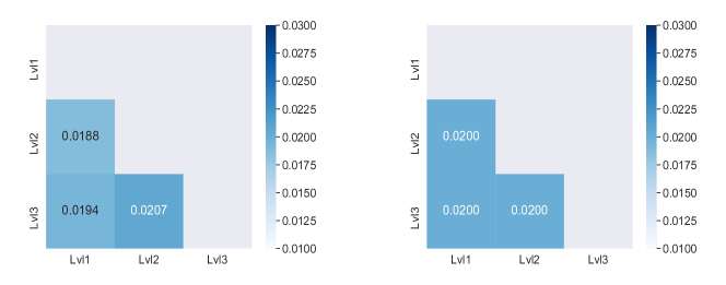
Figure 1: Estimated covariance matrices for OR. Left: Covariance matrix generated from the Convex GL pseudo-counts; Right: Covariance matrix generated from the Solved Hamling pseudo-counts.

There are small differences between the individual entries in Figure 1. These differences are in fact what cause the estimates in Table 2 to vary slightly between the GL and Hamling-based methods. An interesting artifact here is that the Convex GL covariance matrix has different entries, whereas the entries of the Solved Hamling covariance matrix are identical (to the 10th digit or so). This curiosity is due to the fact that Hamling uses reported variances to create the pseudo-counts (see Section 2.1), and in this example, the data report very similar variance values of log-odds estimates.

Next, we run a similar test on relative risks, using the alcohol and colorectal cancer data and results in [10]. We present a summary of the adjusted estimates obtained by our methods and by the methods of GL and Hamling. We use data directly from dosresmeta, specifically the alcohol_crc dataframe, and analyze the subset id author atm. In Table (4) we present the least-squares estimates, similar to what was shown above.

Table 4: Estimates and variances table–log-relative risks.

Method	$\hat{\beta}$	Variance
Unadjusted	-0.00294	1.5865e-05
GL	0.0071	1.5176e-05
Convex GL	0.0071	1.5166e-05
Hamling	0.0063	1.5490e-05
Solved Hamling	0.0063	1.5436e-05

Once again we see small numerical differences in variance estimates, with our estimates using high precision on the equation solves. We also see a larger difference between the estimates obtained by GL vs. Hamling, a direct consequence of the different parametrizations.

We provide a summary of case pseudo-counts generated by each method in Table 5.The pseudo-count estimates within method families are close; while counts between GL and Hamling methods match in some groups but differ in others, causing the differences observed in estimate values in Table 4.

Table 5: Pseudo-count table–log-relative risk.

Method	$a_{0}$	$A_{1}$	$A_{2}$	$A_{3}$	$A_{4}$	$A_{5}$
GL	26.5957	34.0061	42.8532	33.3584	17.9492	29.2359
Convex GL	26.5973	34.0061	42.8532	33.3583	17.9492	29.2359
Hamling	26.4495	39.5129	44.2940	31.6140	15.3332	22.6277
Solved Hamling	26.4087	39.4526	44.2234	31.5706	15.3105	22.5738

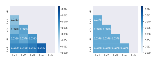
Figure 2: Estimated covariance matrices for RR. Left: Covariance matrix generated from the Convex GL pseudo-counts; Right: Covariance matrix generated from the Solved Hamling pseudo-counts. Both cases are with respect to the relative risk regime.

Covariance matrices obtained from pseudo-counts generated by our Convex GL and Solved Hamling methods are shown in Figure 2. We again see identical entries in the covariance matrix produced from Hamling. The differences in covariance values between the matrices explain the differences in estimates values in Table 4.

We now continue to the avoidable failure modes, providing simple OR examples where the original GL and Hamling methods fail but our Convex GL and Solved Hamling methods succeed.

5.2 Original method failure and Corrected success

In this section we produce simple failure modes for original GL and Hamling methods, and show that new methods work on these cases, as expected from the theoretical results. This is reassuring to practitioners running large numbers of analyses; the need to re-initialize current methods and potential quiet failures of the Hamling method can both be avoided with straightforward modifications. To demonstrate the failure modes, we perturb the alcohol_cvd data from dosresmeta.

5.2.1 GL method failure

Using the method of GL first, we change the number of subjects at each exposure level in the alcohol_cvd dataset to be a function of the number of cases in the same dataset at the corresponding exposure levels. Namely, we modify the number of subjects to be

$$N=A+t$$

for integer values $t=\{1,\dots,20\}$. The lower the $t$, the more extreme the situation, corresponding to very few controls in each group. We use each $N$ as input data to the standard GL routine to construct pseudo-counts using the GL method. For $t\leq 13$, the original GL method in dosresmeta fails.

In the cases of failure, even though the initial $A$ is feasible, GL iterations run afoul of the logarithmic terms in the dosresmeta implementation for low $t$. For $t\geq 14$, this issue disappears. The entire problem is avoided when we use the convex GL approach, which succeeds in all cases. We give a visualization in Figure 3.

Figure 3: Convergence plot of GL for different values of $t$.

The new Convex GL method succeeds even in the extreme case when $t=1$. We compare the covariance matrix for $N^{1}=A+1$ compared to the covariance matrix GL obtains on the original data in Figure 4. We see that the covariance matrices returned for the original and perturbed data are fairly close, suggesting that correlations are well-behaved in such cases and underscoring the need for a robust method. In other words, results for the GL will likely be useful even for small studies when we have very few controls.

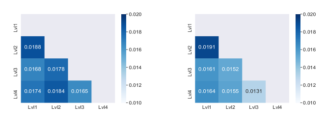
Figure 4: Comparison of GL covariance matrices for original data vs. perturbed data. Left: Covariance matrix generated from the Convex GL pseudo-counts on original data for alcohol; Right: Covariance matrix generated from the Convex GL pseudo-counts on $N^{1}=A+1$, a hypothetical where there is only one control in every group. The original GL method [6] fails on the hypothetical example shown on the right.

5.2.2 Hamling method failure

The Hamling method fails when default initialization fails to guarantee positivity of all denominators $V_{i}-\frac{1}{a_{0}}-\frac{1}{b_{0}}$. For example, the Hamling initialization used by dosresmeeta can be broken by feeding small $V_{i}$ as the data. In this case, the dosresmeta Hamling approach returns negative pseudo-counts, and correlations computed using these counts.

To show this failure mode, we alter the alcohol_cvd dataset in dosresmeta by changing the reported variances to be

$$\hat{V}={\left(\mathrm{NA},0.001,0.01,0.2,0.9\right)}$$

where the NA is a placeholder for the reference exposure level. Passing this data into the hamling method in dosresmeta, we obtain negative values in the estimated counts for cases and non-cases at the first level of exposure, as shown in Table 6.

Table 6: Pseudo-count table–broken Hamling Example.

Method	$a_{0}$	$A_{1}$	$A_{2}$	$A_{3}$	$A_{4}$
Hamling	189.7	-207.5	514.2	8.6	2.2
Solved Hamling	2897.8	2976.1	157.2	31.5706	9.2

The method of Hamling fails silently, since it then uses the negative values to compute the covariance matrix. To study the downstream effects, we compare the covariance matrices constructed by dosresmeta from the wrong pseudo-counts generated by the original Hamling method with those generated by the solved Hamling method in Figure 5. The solved Hamling method obtains an order of magnitude smaller correlation across the subgroups. This means that when Hamling fails quietly, it will provide estimates that deviate further from the uncorrected estimates compared to the correctly solved formulation.

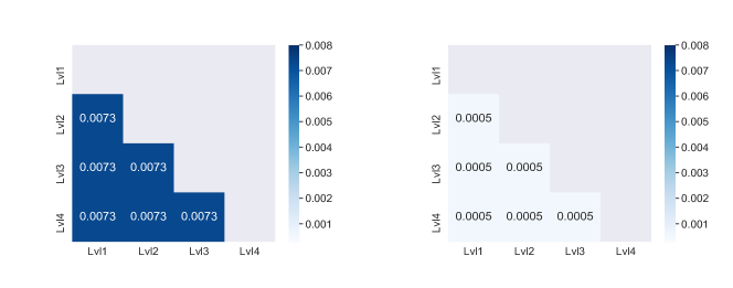
Figure 5: Comparison between covariance matrices generated by Hamling from wrong pseudo-counts and correct pseudo-counts. Left: Covariance matrix generated from the negative Hamling pseudo-counts; Right: Covariance matrix generated from the Solved Hamling pseudo-counts. The correct values result in a much smaller between-level covariance than the incorrect values in this example.

In Figure 6 we extend this example to study the range of the failure mode as a function of the scale of variance values. For simplicity we vary only the first element of $\hat{V}$. We then assess whether there are any negative values in the constructed pseudo-counts for cases $A$ by the Hamling method. As can easily be verified, the variance values below $10^{-3}$ in the first numerical coordinate produce negative values in $A$. Obviously for smaller estimates the method still fails, but such small variances correspond to huge sample sizes that are unlikely to occur in practice. The variance values greater than $10^{-3}$ produce only positive values, even beyond 1. This shows clearly how the Hamling method fails for small enough variance values given default initialization in dosresmeta, and can be fixed easily by using the startegy discussed in Section 4.

Figure 6: Negative value generation in pseudo-cases for different values of variance in the first exposure level.

To fix the problem we use the initialization suggested by the theoretical analysis. Specifically, we construct the initialization parameters $a_{0},b_{0}$ as

$$(a_{0},b_{0})={\left(\frac{10}{\min(v)},\frac{10}{\min(v)}\right)}.$$

The underlying idea is that the large initialization ensures the denominators of $A_{i}$ and $B_{i}$ in equations (3) remain positive, ensuring all counts are positive. This works well numerically, and does not break regardless of the $v_{i}$ values. This provides empirical support for the proof technique given in Theorem 4.2.

In the next section, we study the unavoidable failure mode of Hamling for relative risks.

5.3 Hamling Failure for OR

We review the counter-example presented in Section 4

$$R_{1}=0.9328,R_{2}=0.062,p=0.1,z=1.1.$$

This example was obtained by violating the conditions presented in Theorem 4.3 for the equivariant case. The failure corresponds to obtaining a negative discriminant in the quadratic formula for the ratio $c=\frac{a_{0}}{b_{0}}$, and means that a solution cannot exist, regardless of reported (equal) variances. To see this bear out in practice we make a simple choice

$$v_{1}=v_{2}=1.0.$$

Running dosresmeta on this example gives us results in Table 7.

Table 7: Hamling Results for RR Counter-Example.

$A$	$N$
1.4	1.3
$-1.1\times 10^{-5}$	$-1.1\times 10^{-5}$
$0.88$	$13.3$

We see negative values for $A$ and $N$, a problem for any situation, and $a_{0}>b_{0}$, which is impossible for RR. These issues still can still occur for a candidate solution to the equations (16). However, the claim we made is stronger, that is, a solution that satisfies the six equations corresponding to $p,z,R_{1},R_{2},v_{1},v_{2}$ cannot exist. When we review the dosresmeta result with respect to these six equations, we find that in fact, two of the six are not satisfied:

$$R_{1}(A,N) =0.93,\quad R_{2}(A,N)=0.062,\quad v_{2}(A,N)=1.0,\quad p(A,N)=0.1;$$

$$v_{1}(A,N) =-0.05;\quad z(A,N)=6.33.$$

In contrast to the previous examples, there is no way to fix this; we know from the proof of Theorem 4.3 that no solutions can exist to this example.

6 Conclusion

In this paper we have taken a closer look at the methods of GL [6] and Hamling [8].

We have shown that the GL approach lends itself to a reformulation to minimizing a convex model, for both ORs and RRs. In both cases we can avoid all numerical difficulty and guarantee convergence to the unique optimal point for any feasible data inputs. This was a rather surprising finding that initially motivated us to write the paper. The convex loss that emerged when we integrated the optimality conditions is the entropic distance function, an object that appears in other areas of mathematics and statistics; in particular is heavily used in optimal transport [16]. An unexplored consequence of the connection to convex models is that it is now easy to include side information (if such information is available to modelers) through the use of linear equality and inequality constraints on the pseudo-counts $A$. As long as there is a feasible $A$, the proof theory in this paper guarantees a unique solution, and modifying the formulation is straightforward in cvxpy. We leave further exploration of this idea to future work.

For the Hamling method, the story is more complicated. In the case of OR, we were able to show that the Hamling equations always have a solution. In fact we obtained a closed form solution for the equivariant case (all reported variances equal) and provided a proof by induction for the general case. This means that literally for any observed ORs, variances, $p$, and $z$, we can always find a solution.

In contrast, for RR, there is no guarantee that Hamling will work. We presented a counter-example when there are only two alternative groups. Counter-examples are by nature odd, but nonetheless there is a fundamental difference between RR and OR for Hamling stemming from relying on reported variances. This is curious. Between the methods of GL and Hamling, when faced with many meta-analyses we find the Hamling approach more appealing, since it only needs $p$ and $z$ in addition to reported estimates and variances. Based on the RR failure, we should keep the GL method available should an unavoidable failure mode arise.

We have done our best to make the results as interpretable and clear as possible. We have an implementation for GL and Hamling methods publicly available; and we have shown simple cases where we can break the widely used dosresmeta package using simple examples. Using the insights in this paper, safeguarding estimate available in other packages is a straightforward task. For GL, it is a matter of providing standard optimization guardrails, such as a line search. For Hamling, it is a change in the initialization strategy based on the minimum reported variance.

7 Appendix

In this section, we provide proofs of theorems presented throughout this work.

7.1 Proof of Theorem 3.1

Take $G$ defined as in equation (5). $G$ is continuous on its domain $[0,\infty)^{n}$. First, we show that $G$ is proper, i.e., for some positive values of $A,a_{0},B,b_{0}$, $G(A)\not\equiv+\infty$ and that for any $X\in[0,\infty)^{n},G(X)>-\infty$. For this fact, we need the hypothesis in the statement of the theorem. Let $A$ is the vector of ones of length $n$, i.e., $A=[1,\dots,1]^{\top}$. Since, by hypothesis, $N_{+}>A$ and $n_{0}>a_{0}$, $G(A)<\infty$ inspection. Also by inspection, $G$ is not equal to $-\infty$ for any $A$ in its domain.

Next, $G$ is optimized over the compact set $0\leq A\leq N$. Since, by hypothesis, $N_{+}>A$ and $n_{0}>a_{0}$, $G(A)<\infty$ inspection. Also by inspection, $G$ is not equal to $-\infty$ for any $A$ in its domain. Since $G$ is continuous on the compact domain $0\leq A\leq N$, it attains its minimum and maximum values. Since $G$ is strictly convex, this minimizer must be unique. This completes the proof.

7.2 Proof of Theorem 3.2

Take $H$ as defined in equation (11). This proof will follow the same structure as the proof for Theorem 3.1. We need only show $H$ is proper and that it has compact sublevel sets since $H$ is clearly continuous on the domain $[0,\infty)^{n}$. To show that $H$ is proper, similar to the proof of Theorem (3.1), consider the case when $A$ is the vector of ones of length $n$. By the hypothesis in the statement of Theorem 3.2, $n_{0}>a_{0}$, so that $H$ is finite by inspection. Also by inspection, $H$ is never equal to $-\infty$ on any point in its domain.

Next, we show that $H$ has compact sublevel sets, that is,

$$\mathcal{A}_{\alpha}:=\{A:H(A)\leq\alpha\}$$

are closed and bounded. The closed prpoerty follows immediately by continuity. Next, for a sequence of $X\in[0,\infty)^{n}$, $H(X)\to\infty$ as ${\left\|X\right\|}\to\infty$ since $H$ is a sum of affine functions and entropic distance functions in all coordinates, see equation (9). As ${\left\|X\right\|}\to\infty$, the $x\log x$ terms in $H$ increase faster than linear terms. This implies directly that any sublevel set of $H$ must have an upper bound. Thus, $H$ has compact sublevel sets. In particular, $H$ attains its minimum and maximum for any choice of sublevel set, so in particular we can consider $\alpha=H(1)$, the vector of all ones discussed in the previous paragraph. Once we know $H$ attains its minimum, we also know that the minimum is unique by strict convexity of the entropic distance.

7.3 Proof of Theorem 4.1

To prove the result, we simplify and rewrite the equations

$$\left(V-\frac{1}{a_{0}}-\frac{1}{b_{0}}\right)\frac{1-p}{p}b_{0} =\sum_{i=1}^{n}\left(1+\frac{b_{0}}{a_{0}R_{i}}\right)=n+\frac{b_{0}}{a_{0}}\sum_{i=1}^{n}\frac{1}{R_{i}}=n+\frac{b_{0}}{a_{0}}r_{1}$$

$$\left(V-\frac{1}{a_{0}}-\frac{1}{b_{0}}\right)\left(\frac{1}{zp}b_{0}-a_{0}\right) =\sum_{i=1}^{n}\left(1+\frac{a_{0}R_{i}}{b_{0}}\right)=n+\frac{a_{0}}{b_{0}}\sum_{i=1}^{n}R_{i}=n+\frac{a_{0}}{b_{0}}r_{2}$$

Dividing the equations we obtain

$$\frac{n+\frac{b_{0}}{a_{0}}r_{1}}{n+\frac{a_{0}}{b_{0}}r_{2}}=\frac{\frac{1-p}{p}b_{0}}{\frac{1}{zp}b_{0}-a_{0}}=\frac{\frac{1-p}{p}}{\frac{1}{zp}-\frac{a_{0}}{b_{0}}}$$

Defining now $c=\frac{a_{0}}{b_{0}}$ we have

$$\frac{n+\frac{r_{1}}{c}}{n+cr_{2}}=\frac{\frac{1-p}{p}}{\frac{1}{zp}-c}$$

Multiplying by $c$ we have

$$\frac{r_{1}+nc}{n+r_{2}c}=\frac{(1-p)zc}{1-pzc}$$

The solution is given by

$$c=\frac{npz-nz+n-pr_{1}z\pm\sqrt{D}}{2z(np-pr_{2}+r_{2})}$$

where

$$D =n^{2}p^{2}z^{2}-2n^{2}pz^{2}+2n^{2}pz+n^{2}z^{2}-2n^{2}z+n^{2}-2np^{2}r_{1}z^{2}+2npr_{1}z^{2}+2npr_{1}z+p^{2}r_{1}^{2}z^{2}-4pr_{1}r_{2}z+4r_{1}r_{2}z$$

$$=n^{2}\left(p^{2}z^{2}-2pz^{2}+2pz+z^{2}-z+1\right)$$

$$+n\left(-2p^{2}r_{1}z^{2}+2pr_{1}z^{2}+2pr_{1}z\right)$$

$$+p^{2}r_{1}^{2}z^{2}-4pr_{1}r_{2}z+4r_{1}r_{2}z$$

We want to show that each piece is $\geq 0$. In fact we have

$$p^{2}z^{2}-2pz^{2}+2pz+z^{2}-z+1=z\left((p-1)^{2}z+2p-1\right)+1$$

The minimum with respect to $p$ of the inside expression occurs at $p-1=\frac{-1}{z}$. Plugging in, that gives us

$$z\left(\frac{1}{z}+1-\frac{2}{z}\right)+1=z,$$

so as a result we have

$$n^{2}\left(p^{2}z^{2}-2pz^{2}+2pz+z^{2}-z+1\right)\geq n^{2}z.$$

Next, we have

$$n\left(-2p^{2}r_{1}z^{2}+2pr_{1}z^{2}+2pr_{1}z\right)=n(2r_{1}z)\left((1-p)pz+p\right)\geq 2nr_{1}zp.$$

Finally, we have

$$p^{2}r_{1}^{2}z^{2}-4pr_{1}r_{2}z+4r_{1}r_{2}z=p^{2}r_{1}^{2}z^{2}+4(1-p)r_{1}r_{2}z\geq p^{2}r_{1}^{2}z^{2}$$

Putting everything together, we get

$$D\geq n^{2}z+2nr_{1}zp+p^{2}r_{1}^{2}z^{2}=z(n^{2}+2nr_{1}p+p^{2}r_{1}^{2}z)\geq 0.$$

Thus a solution always exists.

To see that only one solution is positive, recall the form of the solution:

$$c=\frac{npz-nz+n-pr_{1}z\pm\sqrt{D}}{2z(np-pr_{2}+r_{2})}$$

We can observe that

$$n^{2}\left(p^{2}z^{2}-2pz^{2}+2pz+z^{2}-z+1\right)-(n(z(p-1)+1))^{2}=n^{2}z$$

and as a result

$$\sqrt{D}-(npz-nz+n-pr_{1}z)\geq 0.$$

That means we have

$$c_{2}=\frac{npz-nz+n-pr_{1}z-\sqrt{D}}{2z(np+(1-p)r_{2})}<0<c_{1}=\frac{npz-nz+n-pr_{1}z+\sqrt{D}}{2z(np+(1-p)r_{2})}.$$

Plugging $c_{1}$ in to the first equation, we have

$$b_{0}=\frac{1}{V}\left(\frac{p}{1-p}\left(n+\frac{r_{1}}{c}\right)+1+\frac{1}{c_{1}}\right),\quad a_{0}=c_{1}b_{0}.$$

and we have found the unique positive solution. This completes the proof.

7.4 Proof of Theorem 4.2

We prove this theorem by induction. For the base case, when $n=1$, the existence of a unique positive solution follows immediately from Theorem  4.1. For the inductive hypothesis, suppose that for a given $n$ for the dimension of our vectors $V$ and $L$, we have the positive solution pair $a_{0}^{n},b_{0}^{n}$ that simultaneously satisfy the system (14). Thus, we have that

$$\frac{1-p}{p}b_{0}^{n} =\sum_{i=1}^{n}\left(1+\frac{b_{0}^{n}}{a_{0}^{n}R_{i}}\right)/\left(V_{i}-\frac{1}{a_{0}^{n}}-\frac{1}{b_{0}^{n}}\right)$$

$$\frac{1}{zp}b_{0}^{n}-a_{0}^{n} =\sum_{i=1}^{n}\left(1+\frac{a_{0}^{n}R_{i}}{b_{0}^{n}}\right)/\left(V_{i}-\frac{1}{a_{0}^{n}}-\frac{1}{b_{0}^{n}}\right).$$

If we continue to the step $n+1$, we add strictly positive terms to the right hand side, and hence we have strict inequalities

$$\begin{split}\frac{1-p}{p}b_{0}^{n}&<\sum_{i=1}^{n+1}\left(1+\frac{b_{0}^{n}}{a_{0}^{n}R_{i}}\right)/\left(V_{i}-\frac{1}{a_{0}^{n}}-\frac{1}{b_{0}^{n}}\right)\\ \frac{1}{zp}b_{0}^{n}-a_{0}^{n}&<\sum_{i=1}^{n+1}\left(1+\frac{a_{0}^{n}R_{i}}{b_{0}^{n}}\right)/\left(V_{i}-\frac{1}{a_{0}^{n}}-\frac{1}{b_{0}^{n}}\right)\end{split}$$ (17)

and without loss of generality, we may assume that $V_{n+1}\geq\min_{i}V_{i}$ so that $V_{n+1}>\frac{1}{a_{0}^{n}}+\frac{1}{b_{0}^{n}}$. Otherwise, we can suitably reorder the terms and apply the inductive hypothesis.

Define the functions $f_{1},f_{2}$ by

$$f_{1}(a_{0},b_{0}) =\frac{1-p}{p}b_{0}-\sum_{i=1}^{n+1}\left(1+\frac{b_{0}}{a_{0}R_{i}}\right)/\left(V_{i}-\frac{1}{a_{0}}-\frac{1}{b_{0}}\right)$$

$$f_{2}(a_{0},b_{0}) =\frac{1}{zp}b_{0}-a_{0}-\sum_{i=1}^{n+1}\left(1+\frac{a_{0}R_{i}}{b_{0}}\right)/\left(V_{i}-\frac{1}{a_{0}}-\frac{1}{b_{0}}\right).$$

The remaining work is focused on finding the $a_{0}^{n+1},b_{0}^{n+1}$ such that $f_{1}(a_{0}^{n+1},b_{0}^{n+1})=f_{2}(a_{0}^{n+1},b_{0}^{n+1})=0$, and is separated into two steps:

1. Show that we can find points $(a_{0}^{1},b_{0}^{1})$, $(a_{0}^{2},b_{0}^{2})$, $(a_{0}^{3},b_{0}^{3})$ with

   $$f_{1}(a_{0}^{1},b_{0}^{1})>0,\quad f_{2}(a_{0}^{1},b_{0}^{1})>0,$$

   $$f_{1}(a_{0}^{2},b_{0}^{2})>0,\quad f_{2}(a_{0}^{2},b_{0}^{2})<0,$$

   and

   $$f_{1}(a_{0}^{3},b_{0}^{3})<0,\quad f_{2}(a_{0}^{3},b_{0}^{3})>0.$$

   These points, along with $(a_{n},b_{n})$ from the inductive hypothesis, are shown in Figure 7 and the four points set up continuation arguments used in Step 2.

2. Show that, by continuity of the solution maps, either case above leads to the existence of $(a_{0}^{n+1},b_{0}^{n+1})$ simultaneously satisfying $f_{1}=f_{2}=0$.

Step 1 proof:

First, we observe that

$$\lim_{a_{0}\uparrow\infty}f_{1}(a_{0},b_{0})=\frac{1-p}{p}b_{0}-\sum_{i=1}^{n+1}\frac{1}{V_{i}-\frac{1}{b_{0}}}.$$

As long as we take $b_{0}^{1}>2\max\left(V,\frac{p}{1-p}2\sum_{i=1}^{n+1}\frac{1}{V_{i}}\right)$ where $V=\max_{i}V_{i}$, we can then find a large enough value $a_{0}^{1}$ satisfying $f_{1}(a_{0}^{1},b_{0}^{1})>0$. Next, we have

$$\lim_{a_{0}\uparrow\infty}f_{2}(a_{0},b_{0})=-\infty$$

for any $b_{0}$, so in particular we can select a large enough $a_{0}^{1}$ with $f_{2}(a_{0}^{1},b_{0}^{1})<0$ and $f_{1}(a_{0}^{1},b_{0}^{1})>0$. This gives us a point in the lower-right quadrant of Figure 7.

Now we observe that

$$\lim_{b_{0}\uparrow\infty}f_{2}(a_{0},b_{0})=\infty$$

along the path $a_{0}=\frac{1}{2}b_{0}$. Along this same path, we have

$$\lim_{b_{0}\uparrow\infty}f_{1}(a_{0},b_{0})=\infty$$

as well. We can thus select a large enough value $b_{0}^{2}$ and $a_{0}^{2}=\frac{1}{2}b_{0}^{2}$ for which $f_{1}(a_{0}^{2},b_{0}^{2})>0$ and $f_{2}(a_{0}^{2},b_{0}^{2})>0$. This gives us the point in the upper-right quadrant of Figure 7.

Next, consider $0<\epsilon<<1$ and take

$$b_{0}=\frac{1}{\epsilon^{2}},\quad a_{0}=\frac{1}{V_{\min}-\epsilon-\epsilon^{2}}$$

With these definitions, we have

$$f_{2}(\epsilon)\geq\frac{1}{zp\epsilon^{2}}-\frac{1}{V_{\min}-\epsilon-\epsilon^{2}}-(n+1)\left(1+\frac{\epsilon^{2}R_{i}}{V_{\min}-\epsilon-\epsilon^{2}}\right)\frac{1}{\epsilon}>0$$

$$f_{1}(\epsilon)<\frac{1-p}{p\epsilon}-\sum_{i=1}^{n+1}\left(1+\frac{V_{\min}-\epsilon-\epsilon^{2}}{\epsilon^{2}}\right)\frac{1}{\epsilon}<0$$

for small $\epsilon$. Thus for $0<\epsilon<<1$ we get a point $(a_{0}^{3},b_{0}^{3})$ with $f_{2}>0$ and $f_{1}<0$. This gives us a point in the upper left quadrant of Figure 7.

Finally, by the inductive hypothesis, we have $f_{1}(a_{0}^{n},b_{0}^{n})<0$ and $f_{2}(a_{0}^{n},b_{0}^{n})<0$, which gives us a point in the lower left quadrant of Figure 7.

Figure 7: Note the generic form ($a_{0},b_{0}$) is shorthand for $(f_{1}(a_{0},b_{0}),f_{2}(a_{0},b_{0}))$. The point $(a_{0}^{n+1},b_{0}^{n+1})$ serves as desired solution point to complete the proof.

Step 2 Proof:

To show that there is a point $(a_{0}^{n+1},b_{0}^{n+1})$ such that the inequalities (17) become equalities, we create separate interpolations relying on the intermediate value theorem (IVT) [12].

Consider the points $(a_{0}^{n},b_{0}^{n})$ and $(a_{0}^{1},b_{0}^{1})$ and the convex combination

$$p_{\lambda}=\lambda(a_{0}^{n},b_{0}^{n})+(1-\lambda)(a_{0}^{1},b_{0}^{1})$$

We have $f_{1}(p_{1})<0,f_{1}(p_{0})>0$, so by the IVT there is a $\lambda\in(0,1)$ with $f_{1}(p_{\lambda})=0$.

If $f_{2}(p_{\lambda})>0$, we proceed to Case 1 below. If $f_{2}(p_{\lambda})<0$, we have a point of intersection below the $f_{1}$ axis, as shown in Figure 8. We then apply IVT to $(a_{0}^{3},b_{0}^{3})$ and $(a_{0}^{2},b_{0}^{2})$. If the crossing point obtained from the IVT is above the $f_{1}$ axis, we proceed to Case 2 below, and if it is below the $f_{1}$ axis, we proceed to Case 1 below.

• $f_{2}(p_{\lambda})>0$ or IVT applied to $(a_{0}^{3},b_{0}^{3})$ and $(a_{0}^{2},b_{0}^{2})$ yields a point below the $f_{1}$ axis. In either case, applying the IVT twice, we obtain two points along the $f_{1}$ axis, as shown in Figure 9, with opposite signs along $f_{1}$. The constraint $f_{2}=0$ is easily incorporated into $f_{1}$, which becomes

  $$f_{3}(a_{0},b_{0})=(1-p)z\left(a_{0}+\sum_{i=1}^{n+1}\left(1+\frac{a_{0}R_{i}}{b_{0}}\right)/\left(V_{i}-\frac{1}{a_{0}}-\frac{1}{b_{0}}\right)\right)-\sum_{i=1}^{n+1}\left(1+\frac{a_{0}R_{i}}{b_{0}}\right)/\left(V_{i}-\frac{1}{a_{0}}-\frac{1}{b_{0}}\right)$$

  Clearly $f_{3}$ has opposite signs for the two points of intersection in Figure 9, and applying IVT again we find the point $(a_{0}^{n+1},b_{0}^{n+1})$.

• In this case, we have successfully found two points with $f_{1}=0$, and opposite signs with respect to $f_{2}$. Just as in the previous case, we can explicitly incorporate the constraint $f_{1}=0$ into $f_{2}$, to obtain

  $$f_{4}(a_{0},b_{0})=\frac{1}{zp(1-p)}\sum_{i=1}^{n+1}\left(1+\frac{b_{0}}{a_{0}R_{i}}\right)/\left(V_{i}-\frac{1}{a_{0}}-\frac{1}{b_{0}}\right)-a_{0}-\sum_{i=1}^{n+1}\left(1+\frac{a_{0}R_{i}}{b_{0}}\right)/\left(V_{i}-\frac{1}{a_{0}}-\frac{1}{b_{0}}\right)$$

  Clearly $f_{4}$ has opposite signs now for the two crossing points shown on the $f_{2}$ axis of Figure 8, and by IVT, we have existence of $(a_{0}^{n+1},b_{0}^{n+1})$.

Figure 8: The points and their associated continuous deformations (the colored lines) according to Case 1. Note the generic form ($a_{0},b_{0}$) is shorthand for $(f_{1}(a_{0},b_{0}),f_{2}(a_{0},b_{0}))$.

Figure 9: The points and their associated continuous deformations (the colored lines) according to Case 2 in the $f_{1}-f_{2}$ plane. Note the generic form $(a_{0},b_{0})$ is shorthand for $(f_{1}(a_{0},b_{0}),f_{2}(a_{0},b_{0}))$.

7.5 Proof of Theorem 4.3

To prove the result, we simplify and rewrite the equations

$$\left(V_{i}-\frac{1}{a_{0}}+\frac{1}{b_{0}}\right)\frac{1-p}{p}b_{0} =\sum_{i=1}^{n}\left(\frac{b_{0}}{a_{0}R_{i}}-1\right)=\frac{b_{0}}{a_{0}}\sum_{i=1}^{n}\frac{1}{R_{i}}-n=\frac{b_{0}}{a_{0}}r_{1}-n$$

$$\left(V_{i}-\frac{1}{a_{0}}+\frac{1}{b_{0}}\right)\left(\frac{1}{zp}b_{0}-a_{0}\right) =\sum_{i=1}^{n}\left(1-\frac{a_{0}R_{i}}{b_{0}}\right)=n-\frac{a_{0}}{b_{0}}\sum_{i=1}^{n}R_{i}=n-\frac{a_{0}}{b_{0}}r_{2}$$

Dividing the equations we obtain

$$\frac{\frac{b_{0}}{a_{0}}r_{1}-n}{n-\frac{a_{0}}{b_{0}}r_{2}}=\frac{\frac{1-p}{p}b_{0}}{\frac{1}{zp}b_{0}-a_{0}}=\frac{\frac{1-p}{p}}{\frac{1}{zp}-\frac{a_{0}}{b_{0}}}$$

Defining now $c=\frac{a_{0}}{b_{0}}$ we have

$$\frac{\frac{r_{1}}{c}-n}{n-cr_{2}}=\frac{\frac{1-p}{p}}{\frac{1}{zp}-c}$$

with the inherited constraint that $c<1$, since $a_{0}<b_{0}$ by definition. Multiplying by $c$ we have

$$\frac{r_{1}-nc}{n-r_{2}c}=\frac{(1-p)zc}{1-pzc}$$

The solution is given by

$$c=\frac{n(z-pz+1)+pr_{1}z\pm\sqrt{D}}{2z(np+(1-p)r_{2})}$$

where

$$D=(n(pz-z-1)-r_{1}zp)^{2}-4r_{1}(nzp+r_{2}z-r_{2}pz).$$

By inspection the coefficient for $n^{2}$ is given by

$$(pz-z-1)^{2},$$

which is always positive. The coefficient for $n$ is given by

$$(-2(pz-z-1)-4)zpr_{1}=2zpr_{1}(z-pz-1)$$

This term is non-negative exactly when $(1-p)z\geq 1$. Finally, the constant term is given by

$$r_{1}^{2}z^{2}p^{2}+4r_{1}r_{2}z(p-1).$$

The condition for when this term is non-negative can also be written in terms of $(1-p)z$:

$$(1-p)z\geq\left(\frac{1-p}{p}\right)^{2}4r_{2}.$$

It is easy to find a counter-example when these conditions are violated, and where $D<0$.

$$n=2,\quad p=0.1,\quad z=1.1,\quad r_{1}=31.9,\quad r_{2}=1.$$

This yields $D=-33.4$, so there is no solution. In this case, $(1-p)z=0.99$, while $\frac{(1-p)^{2}}{p^{2}}4r_{2}=324$, so both inequalities are violated, the latter significantly. The result is easily achievable, since we just want to find $\alpha$ with

$$\frac{2}{1-\alpha}+\frac{2}{\alpha}=31.9.$$

This gives us

$$R_{1}=.9328,R_{2}=.0672.$$

References

- [1] Stephen Boyd and Lieven Vandenberghe. Convex optimization. Cambridge university press, 2004.
- [2] Alessio Crippa and Nicola Orsini. Multivariate dose-response meta-analysis: The dosresmeta R package. Journal of Statistical Software, Code Snippets, 72(1):1–15, 2016.
- [3] Xiaochen Dai, Gabriela F Gil, Marissa B Reitsma, Noah S Ahmad, Jason A Anderson, Catherine Bisignano, Sinclair Carr, Rachel Feldman, Simon I Hay, Jiawei He, et al. Health effects associated with smoking: a burden of proof study. Nature medicine, 28(10):2045–2055, 2022.
- [4] Walter Gautschi. Numerical analysis: an introduction. Birkhauser Boston Inc., USA, 1997.
- [5] Michael Grant, Stephen Boyd, and Yinyu Ye. Disciplined convex programming. Springer, 2006.
- [6] Sander Greenland and Matthew P. Longnecker. Methods for trend estimation from summarized dose-response data, with applications to meta-analysis. American journal of epidemiology, 135 11:1301–9, 1992.
- [7] Anna-Bettina Haidich. Meta-analysis in medical research. Hippokratia, 14(Suppl 1):29, 2010.
- [8] Jan Hamling, Peter Lee, Rolf Weitkunat, and Mathias Ambühl. Facilitating meta-analyses by deriving relative effect and precision estimates for alternative comparisons from a set of estimates presented by exposure level or disease category. Statistics in medicine, 27(7):954–970, 2008.
- [9] Haley Lescinsky, Ashkan Afshin, Charlie Ashbaugh, Catherine Bisignano, Michael Brauer, Giannina Ferrara, Simon I Hay, Jiawei He, Vincent Iannucci, Laurie B Marczak, et al. Health effects associated with consumption of unprocessed red meat: a burden of proof study. Nature Medicine, 28(10):2075–2082, 2022.
- [10] Nicola Orsini, Ruifeng Li, Alicja Wolk, Polyna Khudyakov, and Donna Spiegelman. Meta-analysis for linear and nonlinear dose-response relations: examples, an evaluation of approximations, and software. American journal of epidemiology, 175(1):66–73, 2012.
- [11] Christian Razo, Catherine A Welgan, Catherine O Johnson, Susan A McLaughlin, Vincent Iannucci, Anthony Rodgers, Nelson Wang, Kate E LeGrand, Reed JD Sorensen, Jiawei He, et al. Effects of elevated systolic blood pressure on ischemic heart disease: a burden of proof study. Nature medicine, 28(10):2056–2065, 2022.
- [12] Walter Rudin et al. Principles of mathematical analysis, volume 3. McGraw-hill New York, 1964.
- [13] Carsten Oliver Schmidt and Thomas Kohlmann. When to use the odds ratio or the relative risk? International journal of public health, 53(3):165, 2008.
- [14] Jeffrey D Stanaway, Ashkan Afshin, Charlie Ashbaugh, Catherine Bisignano, Michael Brauer, Giannina Ferrara, Vanessa Garcia, Demewoz Haile, Simon I Hay, Jiawei He, et al. Health effects associated with vegetable consumption: a burden of proof study. Nature medicine, 28(10):2066–2074, 2022.
- [15] Endre Süli and David F. Mayers. An Introduction to Numerical Analysis. Cambridge University Press, 2003.
- [16] Cédric Villani et al. Optimal transport: old and new, volume 338. Springer, 2009.
- [17] Peng Zheng, Aleksandr Aravkin, Christopher Murray, et al. The burden of proof studies: assessing the evidence of risk. Nature Medicine, 28(10):2038–2044, 2022.