Open-system eigenstate thermalization in a noninteracting integrable model

Abstract

We study thermalization in isolated quantum systems from an open quantum systems perspective. We argue that for a small system connected to a macroscopic bath, the system observables are thermal if the combined system-bath configuration is in an eigenstate of its Hamiltonian, even for fully integrable models (unless thermalization is suppressed by localization due to strong coupling). We illustrate our claim for a single fermionic level coupled to a noninteracting fermionic bath. We further show that upon quenching the system Hamiltonian, the system occupancy relaxes to the thermal value corresponding to the new Hamiltonian. Finally, we demonstrate that system thermalization also arises for a system coupled to a bath initialized in a typical eigenstate of its Hamiltonian. Our findings show that chaos and nonintegrability are not the sole drivers of thermalization and complementary approaches are needed to offer a more comprehensive understanding of how statistical mechanics emerges.

I Introduction

Many states of matter occurring in nature can be characterized as thermal equilibrium states, i.e., the expected values of their observables can be characterized using a single or a few intensive thermodynamic parameters (e.g., temperature or chemical potentials of particles). The emergence of thermal behavior has been explained using the concept of statistical ensemble (e.g., microcanonical, canonical, or grand canonical). For example, within the microcanonical picture, the thermal state is described as a statistical mixture of equally probable microstates that have the same energy.

Since the time of Boltzmann, the justification of the statistical assumption that a system’s microstates are equally probable, based on the principles of classical or quantum mechanics, has been a subject of intense debate. A proposed bridge between mechanics and statistical behavior is the ergodic hypothesis [1] which states that long-time averages of observables for a dynamical system correspond to microcanonical ensemble averages. This property has been proven for a few model mechanical systems [2, 3, 4, 5]. One approach to the origin of ergodicity and thermalization, associated with the Brussels school, is based on the assumption that the dynamics of the microscopic system is chaotic [6, 7]. Chaotic behavior is associated with nonintegrability of the system dynamics, i.e., a situation in which the number of conserved quantities is smaller than the number of degrees of freedom. However, as shown by the Kolmogorov–Arnold–Moser theorem [8, 9, 10], even nonintegrable systems are not necessarily ergodic. This is illustrated, e.g., by the famous Fermi–Pasta–Ulam–Tsingou problem [11, 12].

In the quantum context, investigations of the origin of statistical mechanics gave rise to the field of pure-state statistical mechanics, which postulates and justifies the thermal behavior of individual quantum pure states [13]. One of the most successful approaches in this area is based on the eigenstate thermalization hypothesis (ETH) [14, 15, 16, 17], which is similar to the classical postulate of chaoticity of the microscopic dynamics. A strong version of this hypothesis states that observables take thermal values for every eigenstate of the Hamiltonian. ETH has been numerically verified for a wide range of quantum systems far from integrability (for references, see Ref. [16]), while it is violated for integrable systems, whose observables are rather described by the so-called generalized Gibbs ensembles [18, 19, 20]. Furthermore, ETH can be used not only to explain the thermal behavior of static observables but also certain aspects of nonequilibrium dynamics. For example, it justifies thermalization after quench, that is, a situation in which, after changing the Hamiltonian at some moment, the observables relax over time to thermal values for the new Hamiltonian [21]. Furthermore, it can also be used to establish the microscopic origin of the second law of thermodynamics and fluctuation theorems [22] or the emergence of nonequilibrium steady states [23, 24].

ETH has been shown to be necessary to explain certain aspects of thermalization, such as equilibration with thermal baths [25] or universality of dynamics after Hamiltonian quench [26]. However, many features of thermal behavior can also be observed for systems that do not obey ETH, including integrable systems. Approaches to explain the origin of thermalization without invoking nonintegrability are mostly akin to the arguments of Boltzmann, who rationalized thermal behavior by postulating the typicality of initial conditions for a system consisting of many degrees of freedom [27]. Following this direction, Chakraborti et al. [28] observed the thermal behavior of a gas of noninteracting classical particles for typical individual microstates randomly sampled from the canonical ensemble. The other approach postulates the typicality of measured observables rather than initial conditions. In this spirit, Khinchin [29] has shown that functions expressed as sums of many independent degrees of freedom (e.g., coordinates of noninteracting particles) tend to thermalize due to the law of large numbers, without any assumption about the ergodicity of the microscopic dynamics. Mazur and van der Linden [30] later generalized this result to short-range interacting particles. Motivated by this, Baldovin et al. [31] demonstrated thermalization of collective observables in an anharmonic but integrable Toda chain even for very untypical initial conditions. Later studies [32, 33] have even demonstrated the thermalization of certain observables in a fully harmonic oscillator chain.

In the quantum context, typicality arguments have been employed in von Neumann’s ergodic theorem [34, 35]. It states that for typical observables, for every pure state with a narrow energy distribution (i.e., a superposition of energy eigenstates from a microcanonical shell), the time average of the observable corresponds to its microcanonical average. This theorem was later generalized by Reimann [36], who relaxed some of its original assumptions. However, it has been shown that von Neumann’s proof involves an assumption which is essentially equivalent to ETH [37]. The other concept is canonical typicality [38, 39, 40, 41], which states that typical pure states with a narrow energy distribution predict the same reduced states of small subsystems as the microcanonical ensemble. A related but different concept is weak ETH, which postulates that subsystem thermalization is also observed for typical (though not all) individual energy eigenstates. It has been proven for translationally invariant short-range interacting spin systems, including integrable ones [42, 22]. We note that the applicability of these concepts is often limited compared to “strong” ETH. For example, integrable systems obeying weak ETH do not exhibit thermalization after Hamiltonian quench [42, 43]. Still, Refs. [44, 45] observed thermalization after quench in certain nonintegrable systems that violate ETH.

Furthermore, certain features of thermalization have been observed even for noninteracting systems. Magán [46] observed thermalization of local observables for typical many-body eigenstates of random noninteracting fermionic Hamiltonians. Refs. [47, 48, 43] observed subsystem thermalization for translationally invariant systems of noninteracting fermions. This thermalization is suppressed by the presence of a disorder that breaks the translational invariance [48]. Refs. [49, 50] demonstrated thermalization of one- and few-body observables in chaotic quadratic Hamiltonians. Finally, in the nonequilibrium context, it was shown that in translationally invariant fermionic chains the charge distribution tends to thermalize at the coarse-grained (macroscopic) level even for very untypical initial conditions, even though the fine-grained (microscopic) observables do not thermalize [51, 52].

However, the problem of pure-state thermalization in integrable and noninteracting models has hardly been analyzed from the open quantum system perspective, where the splitting of the total system into a small system and a macroscopic bath specifies the choice of the considered observables. As an exception, Usui et al. [53] recently demonstrated the emergence of nonequilibrium steady states and long-time thermalization of macroscopic bath observables for a fermionic impurity coupled to noninteracting baths initialized in the pure states randomly sampled from the grand canonical ensemble. Here we address another aspect of that problem by analyzing whether the microscopic system observables are thermalized by individual eigenstates of the total system-bath Hamiltonian. We show that such a thermalization can be observed even in fully integrable noninteracting resonant level model consisting of a single fermionic level coupled to a bath of fermionic levels via a bilinear tunneling Hamiltonian. It is shown that typical many-particle eigenstates of the total Hamiltonian thermalize the system occupancy, i.e., it tends to have the same value as for the thermal state with the same energy and particle number. Specifically, this occurs when the single-particle state corresponding to the occupied state of the system is strongly delocalized over many single-particle eigenstates of the Hamiltonian. Consequently, thermalization may be suppressed by localization induced by formation of the bound states for a strong system-bath coupling. At the same time, no thermalization is observed for occupancies of the bath levels. We further demonstrate that after the quench of the system energy, the system occupancy relaxes to the thermal value for the new Hamiltonian. Finally, we show that thermalization of the system can be induced by the bath initialized in typical eigenstates of its Hamiltonian.

The paper is organized as follows. In Sec. II we present details of the considered model and methods used to describe it. In Sec. III we define several concepts and quantities used throughout the paper. In Secs. IV and V we explore the thermalization of static observables and the thermalization after quench, respectively. In Sec. VI we investigate the system thermalization induced by typical bath eigenstates. Finally, Sec. VII brings conclusions that follow from our results.

II Model and methods

We consider a paradigmatic example of an integrable open quantum system, namely, the noninteracting resonant level described by the Hamiltonian

$$\hat{H}=\epsilon_{0}c^{\dagger}_{0}c_{0}+\sum_{k=1}^{K-1}\epsilon_{k}c_{k}^{\dagger}c_{k}+\sum_{k=1}^{K-1}\left(t_{k}c^{\dagger}_{0}c_{k}+\text{h.c.}\right),$$ (1)

where the index $k=0$ corresponds to the system, while $k\in\{1,\ldots,K-1\}$ to the energy levels in the bath. Here $\epsilon_{k}$ is the level energy, $c^{\dagger}_{k}$ and $c_{k}$ are the creation and annihilation operators, $t_{k}$ is the tunnel coupling between the levels $0$ and $k$, and $K-1$ is the number of energy levels in the reservoir. We further focus on a flat-band model with the bath levels parameterized as $\epsilon_{k}=-W/2+\Delta_{\epsilon}(k-1)$, where $\Delta_{\epsilon}=W/(K-2)$ is the interlevel spacing in the bath, and $W$ is the bath bandwidth. The tunnel couplings are parameterized as $t_{k}=\sqrt{\Gamma/(2\pi\Delta_{\epsilon})}$, where $\Gamma$ is the coupling strength to the bath.

This Hamiltonian can be rewritten in the form

$$\hat{H}=\sum_{kl}\mathcal{H}_{kl}c_{k}^{\dagger}c_{l},$$ (2)

where $\mathcal{H}$ is the matrix representing the single-particle sector of the Hamiltonian. It is defined as

$$\begin{cases}\mathcal{H}_{kk}=\epsilon_{k}&\text{for}\quad k=0,\ldots,K-1,\\ \mathcal{H}_{0k}=\mathcal{H}_{k0}=t_{k}&\text{for}\quad k=1,\ldots,K-1,\\ \mathcal{H}_{kl}=0&\text{otherwise}.\end{cases}$$ (3)

Hamiltonian (1) can be diagonalized to a form

$$\hat{H}=\sum_{k=0}^{K-1}\omega_{k}d^{\dagger}_{k}d_{k},$$ (4)

where the new fermionic operators $d_{k}$ are superpositions of the original operators:

$$d_{k}=\sum_{l=0}^{K-1}a_{lk}c_{l}.$$ (5)

In practice, $\omega_{k}$ is $k$th eigenvalue of the matrix $\mathcal{H}$, and $a_{lk}^{*}$ is the $l$th elements of its $k$th normalized eigenvector. Conversely, original operators can be expressed in terms of the new ones as

$$c_{k}=\sum_{l=0}^{K-1}a_{kl}^{*}d_{l}.$$ (6)

The many-particle eigenstates of the Hamiltonian (1) can be expressed as

$$|E_{i},N_{i}\rangle=(d_{K-1}^{\dagger})^{n_{i,K-1}}\ldots(d_{0}^{\dagger})^{n_{i,0}}|\varnothing\rangle,$$ (7)

where $|\varnothing\rangle$ is the vacuum state. Each eigenstate is associated with a unique combination of level occupancies $n_{i,k}\in\{0,1\}$. $E_{i}=\sum_{k=0}^{K-1}n_{i,k}\omega_{k}$ denotes the eigenstate energy, and $N_{i}=\sum_{k=0}^{K-1}n_{i,k}$ is the particle number. We note that for typical many-particle eigenstates, the occupancies of single-particle eigenstates $d^{\dagger}_{k}|\varnothing\rangle$ are far from being thermal: they can take only values 0 or 1, while thermal occupancies may lie within the range $[0,1]$.

We also consider the case where, at some moment, the Hamiltonian is quenched from the initial form $\hat{H}$ to the final form $\hat{H}^{\prime}$. The new Hamiltonian can be analogously diagonalized as

$$\hat{H}^{\prime}=\sum_{k=0}^{K-1}\nu_{k}f_{k}^{\dagger},$$ (8)

with

$$f_{k}=\sum_{l=0}^{K-1}b_{lk}c_{l},\quad c_{k}=\sum_{l=0}^{K-1}b_{kl}^{*}f_{l}.$$ (9)

To describe the dynamics of the system under the Hamiltonian $\hat{H}^{\prime}$, we use the evolution of operators in the Heisenberg picture. Using the expression above, the operators $c_{k}(t)$ evolve as

$$c_{k}(t)=\sum_{m}b_{km}^{*}f_{m}e^{-i\nu_{m}}=\sum_{m,n}b_{nm}b_{km}^{*}e^{-i\nu_{m}}c_{n}.$$ (10)

It is also be useful to re-express this formula in terms of operators $d_{k}$. Using Eq. (6) one obtains

$$c_{k}(t)=\sum_{l}a_{kl}^{*}(t)d_{l},$$ (11)

where

$$a_{kl}(t)=\sum_{n,m}a_{nl}b_{km}b_{nm}^{*}e^{i\nu_{m}}.$$ (12)

Finally, let us understand the amplitudes $a_{kl}$ and $a_{kl}(t)$ as elements of the matrices $\mathbf{a}$ and $\mathbf{a}(t)$, respectively. Then, using spectral decomposition of the matrix exponent, the equation above can be rewritten in a concise form

$$\mathbf{a}(t)=e^{i\mathcal{H}^{\prime}t}\mathbf{a},$$ (13)

which is very convenient for numerical implementation.

III Definitions

Let us now define certain concepts and quantities used throughout the paper. First, the microcanonical set $\mathcal{W}$ is defined as a set of energy eigenstates $|E_{i},N_{i}\rangle$ with $E_{i}\in[E,E+\Delta E]$ and $N_{i}\in[N,N+\Delta N]$, where $\Delta E$ and $\Delta N$ are small widths of the microcanonical shell. The microcanonical state is defined as an equally weighted mixture of states belonging to the microcanonical set:

$$\rho_{\text{mc}}\equiv\frac{1}{|\mathcal{W}|}\sum_{i\in\mathcal{W}}|E_{i},N_{i}\rangle\langle E_{i},N_{i}|,$$ (14)

where $|\mathcal{W}|$ is the cardinality of the microcanonical set, i.e., the number of its elements. We further define the grand canonical state equivalent to the microcanonical state as

$$\rho_{\text{gc}}\equiv Z^{-1}e^{-\beta(\hat{H}-\mu\hat{N})},$$ (15)

where $\hat{N}=\sum_{K=0}^{K-1}c_{k}^{\dagger}c_{k}$ is the total particle number operator and $Z$ is the normalization constant providing $\text{Tr}(\rho_{\text{gc}})=1$. To provide equivalence with the microcanonical state, the inverse temperature $\beta$ and the chemical potential $\mu$ are chosen such that

$$\text{Tr}(\rho_{\text{gc}}\hat{H})=E\quad\text{and}\quad\text{Tr}(\rho_{\text{gc}}\hat{N})=N.$$ (16)

Following Ref. [54], let us now define the indicator of eigenstate thermalization for the observable $\hat{A}$,

$$I_{\text{mc}}(\hat{A})\equiv\sqrt{\frac{1}{|\mathcal{W}|}\sum_{i\in\mathcal{W}}(\langle\hat{A}\rangle_{i}-\langle\hat{A}\rangle_{\text{mc}})^{2}},$$ (17)

where $\langle\hat{A}\rangle_{i}=\langle E_{i},N_{i}|\hat{A}|E_{i},N_{i}\rangle$ is the expected value of the observable $\hat{A}$ for an individual eigenstate $|E_{i},N_{i}\rangle$, and $\langle\hat{A}\rangle_{\text{mc}}=\text{Tr}(\rho_{\text{mc}}\hat{A})$ is the microcanonical average of this observable. This quantity measures how, typically, the expected value of the observable $\hat{A}$ evaluated for an individual eigenstate differs from its thermal value. In other words, it evaluates how well typical eigenstates belonging to the microcanonical set thermalize the observable $\hat{A}$. Thermalization is indicated by the vanishing of $I_{\text{mc}}(\hat{A})$ in the thermodynamic limit [54].

Let us further define two auxiliary quantities:

$$C(\hat{A},\hat{B})\equiv\frac{1}{|\mathcal{W}|}\sum_{i\in\mathcal{W}}(\langle\hat{A}\rangle_{i}-\langle\hat{A}\rangle_{\text{mc}})(\langle\hat{B}\rangle_{i}-\langle\hat{B}\rangle_{\text{mc}}),$$ (18)

$$\text{Cov}_{\text{mc}}(\hat{A},\hat{B})\equiv\frac{1}{2}\text{Tr}(\rho_{\text{mc}}\{\hat{A}-\langle\hat{A}\rangle,\hat{B}-\langle\hat{B}\rangle\}).$$ (19)

The latter quantity is the covariance of observables in the microcanonical state; in particular, $\text{Cov}_{\text{mc}}(\hat{A},\hat{A})=\text{Var}_{\text{mc}}(\hat{A})$ is the variance of the observable $\hat{A}$. We now make an observation that will later appear to be very useful: when the observables $\hat{A}$ and $\hat{B}$ commute with the Hamiltonian $\hat{H}$, then

$$C(\hat{A},\hat{B})=\text{Cov}_{\text{mc}}(\hat{A},\hat{B}).$$ (20)

This can be easily proven by inserting the definition of the microcanonical state to Eq. (19), and later using the fact that, due to commutation of $\hat{A}$ and $\hat{B}$ with the Hamiltonian, the energy eigenstates $|E_{i},N_{i}\rangle$ are also the eigenstates of $\hat{A}$ and $\hat{B}$, i.e., $\hat{A}|E_{i},N_{i}\rangle=\langle\hat{A}\rangle_{i}|E_{i},N_{i}\rangle$ and $\hat{B}|E_{i},N_{i}\rangle=\langle\hat{B}\rangle_{i}|E_{i},N_{i}\rangle$.

IV Thermalization of static observables

IV.1 Theoretical arguments

We now analyze whether and which observables of the considered system are thermalized by single eigenstates $|E_{i},N_{i}\rangle$. In particular, we focus on the local occupancies of levels $k$ in the original basis. They are denoted as $\langle\hat{p}_{k}\rangle$, where $\hat{p}_{k}=c_{k}^{\dagger}c_{k}$. We use the fact that, for both single eigenstates and for the microcanonical or grand canonical states, the density matrix of the system is diagonal in the basis diagonalizing the Hamiltonian $\hat{H}$. As a consequence, occupancies $\langle\hat{p}_{k}\rangle$ can be expressed in terms of occupancies of single-particle eigenstates:

$$\langle\hat{p}_{k}\rangle=\sum_{l=0}^{K-1}|a_{kl}|^{2}\langle\hat{n}_{l}\rangle,$$ (21)

where $\hat{n}_{k}=d_{k}^{\dagger}d_{k}$. Using Eq. (17), the indicator of thermalization of the observable $\hat{p}_{k}$ can be calculated as

$$I_{\text{mc}}(\hat{p}_{k})=\sqrt{\sum_{lm}|a_{kl}|^{2}|a_{km}|^{2}C(\hat{n}_{l},\hat{n}_{m})},$$ (22)

where $C(\hat{n}_{l},\hat{n}_{m})$ is defined via Eq. (18). We now use the fact that the observables $\hat{n}_{l}$ commute with the Hamiltonian $\hat{H}$. As a consequence, using Eq. (20), the equation above can be rewritten as

$$I_{\text{mc}}(\hat{p_{k}})=\sqrt{\sum_{lm}|a_{kl}|^{2}|a_{km}|^{2}\text{Cov}_{\text{mc}}(\hat{n}_{l},\hat{n}_{m})}.$$ (23)

We now assume that the amplitudes $|a_{kl}|$ are nonnegligible only for a set of levels $l$ whose energies $\epsilon_{l}$ are close to $\epsilon_{k}$ (i.e., the levels resonantly coupled with the level $k$). We further assume that this set is small compared to the set of all levels. Then we make use of the principle of ensemble equivalence which states that the state of a small subsystem of a large system is the same for the microcanonical state and the equivalent grand canonical state. Therefore, we may approximate the indicator $I_{\text{mc}}(\hat{p}_{k})$ by replacing the microcanonical covariances $\text{Cov}_{\text{mc}}(\hat{n}_{l},\hat{n}_{m})$ in Eq. (23) with the grand canonical covariances $\text{Cov}_{\text{gc}}(\hat{n}_{l},\hat{n}_{m})$; they are defined as in Eq. (19), but with $\rho_{\text{mc}}$ replaced by $\rho_{\text{gc}}$. We further note that in the grand canonical state the covariances of occupancies of different single-particle eigenstates vanish: $\text{Cov}_{\text{gc}}(\hat{n}_{l},\hat{n}_{m})=0$ for $l\neq m$. Therefore, the indicator $I_{\text{mc}}(\hat{p}_{k})$ can be approximated as

$$I_{\text{mc}}(\hat{p}_{k})\approx\sqrt{\sum_{l}|a_{kl}|^{4}\text{Var}_{\text{gc}}(\hat{n}_{l})},$$ (24)

where $\text{Var}_{\text{gc}}(\hat{n}_{l})$ is the grand canonical variance of the operator $\hat{n}_{l}$. Finally, using the inequality $\text{Var}_{\text{gc}}(\hat{n}_{l})\leq 1/4$ (which results from the fact that level occupancy is a binary variable), we can approximately bound the indicator $I_{\text{mc}}(\hat{p}_{k})$ as

$$I_{\text{mc}}(\hat{p}_{k})\lessapprox\frac{1}{2}\sqrt{\text{IPR}_{k}},$$ (25)

where $\text{IPR}_{k}$ is the inverse participation ratio for level $k$:

$$\text{IPR}_{k}\equiv\sum_{l=0}^{K-1}|a_{kl}|^{4}.$$ (26)

This quantity is a standard measure of the delocalization of single-particle states $c_{k}^{\dagger}|\varnothing\rangle$ over single-particle eigenstates $d_{l}^{\dagger}|\varnothing\rangle$ [55]. When $\text{IPR}_{k}$ is close to $1$, the state $c_{k}^{\dagger}|\varnothing\rangle$ is strongly localized in a single eigenstate $d_{l}^{\dagger}|\varnothing\rangle$; conversely, when $\text{IPR}_{k}$ scales as 1/K (and thus goes to 0 in the thermodynamic limit), the state $c_{k}^{\dagger}|\varnothing\rangle$ is delocalized over many single-particle eigenstates. Consequently, Eq. (25) implies that occupancies $\langle\hat{p}_{k}\rangle$ are thermalized by typical eigenstates of the system-bath Hamiltonian when states $c_{k}^{\dagger}|\varnothing\rangle$ are strongly delocalized. This reminds us of the result of Khinchin, obtained in the context of classical statistical mechanics: Observables, which can be expressed as a sum of many independent degrees of freedom, tend to thermalize due to the law of large numbers, independent of the details of microscopic dynamics [29]. We also note that the connection between thermalization or equilibration and the inverse participation ratio (or its inverse, known as the effective dimension) has already been recognized in the literature [56, 57, 58, 13].

IV.2 Localization

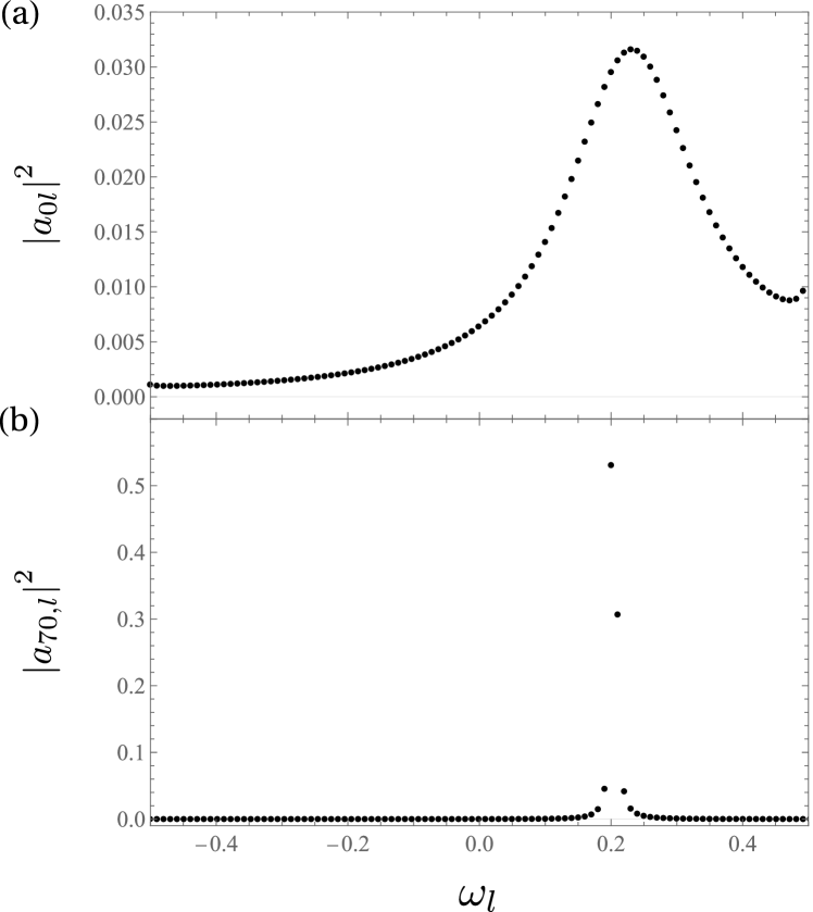
Figure 1: The absolute squares of the amplitudes $a_{kl}$ as a function of the single-particle eigenstate energy $\omega_{l}$ for the system level $k=0$ (a) and the bath level $k=70$ (b). Parameters: $K=100$, $\epsilon_{0}=0.2W$, $\Gamma=0.2W$.

Let us now analyze the localization properties of single-particle states $c_{k}^{\dagger}|\varnothing\rangle$ for the considered model. First, we analyze the distribution of the absolute squares of the amplitudes $a_{0k}$, which quantify the overlaps of states $c_{0}^{\dagger}|\varnothing\rangle$ and $d_{l}^{\dagger}|\varnothing\rangle$. This is plotted in Fig. 1 (a) for $K=100$. One may observe that the state $c_{0}^{\dagger}|\varnothing\rangle$ is delocalized over many eigenstates $d_{l}^{\dagger}|\varnothing\rangle$ with energy close to $\epsilon_{0}$.This is because the system is strongly affected by interaction with many bath levels (providing that the coupling strength $\Gamma$ is neither to weak nor too strong; see a discussion below). According to our theoretical reasoning, this implies thermalization of the system occupancy $\langle\hat{p}_{0}\rangle$; we will demonstrate this numerically in the next subsection.

For comparison, let us now consider the localization properties of the single-particle states $c_{k}^{\dagger}|\varnothing\rangle$ for the bath levels (with $k>0$). Specifically, in Fig. 1 (b) we present the state overlaps for the level $k=70$, that is, the bath level with the energy $\epsilon_{k}$ closest to $\epsilon_{0}$. As can be seen, the state $c_{70}^{\dagger}|\varnothing\rangle$ is strongly localized in just a pair of eigenstates $d_{l}^{\dagger}|\varnothing\rangle$ with the energy closest to $\epsilon_{70}$. This is reasonable, since the bath is only weakly perturbed by a coupling to a small system. As will be shown later, this results in the lack of thermalization of the bath level occupancies.

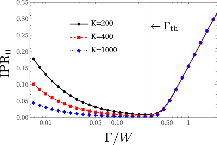
Figure 2: The inverse participation ratio $\text{IPR}_{0}$ as a function of the coupling strength $\Gamma$ for different number of levels $K$. Parameters: $\epsilon_{0}=0.2W$.

We now focus on the localization properties of the single-particle states of the system $c_{0}^{\dagger}|\varnothing\rangle$, by analyzing the inverse participation ratio $\text{IPR}_{0}$. In Fig. 2 we plot this quantity (in the log-linear scale) as a function of the coupling strength $\Gamma$ for different numbers of levels $K$. Interestingly, it exhibits a qualitatively different behavior for $\Gamma$ below and above the localization threshold $\Gamma_{\text{th}}$. The numerical results suggest that this threshold corresponds to the distance of the system energy from the band edge: $\Gamma_{\text{th}}\approx W/2-|\epsilon_{0}|$. Below the threshold, the inverse participation ratio decreases with increasing $\Gamma$ or $K$. This may be explained as follows: The amplitudes $a_{0l}$ are large only for those levels $l$, whose energies are resonant with the system, that is, for which the difference $|\omega_{l}-\epsilon_{0}|$ is of the order of the coupling strength $\Gamma$ (which corresponds to the level broadening due to the system-bath coupling). The number of those levels is proportional to $\Gamma/\Delta_{\epsilon}\propto\Gamma K$, where, to recall, $\Delta_{\epsilon}=W/(K-2)$ is the interlevel spacing in the bath. At the same time, the state overlaps are normalized as $\sum_{l=0}^{K-1}|a_{kl}|^{2}=1$. Thus, individual overlaps $|a_{0l}|^{2}$ scale proportionally to $1/(\Gamma K)$, and their squares $|a_{0l}|^{4}$ scale as $1/(\Gamma K)^{2}$. Consequently, the inverse participation ratio $\text{IPR}_{0}=\sum_{l=0}^{K-1}|a_{0l}|^{4}$ scales as $(\Gamma K)/(\Gamma K)^{2}=1/(\Gamma K)$ (proportionally to the number of significant elements $|a_{0l}|^{4}$ and inversely proportionally to their values). Thus, the inverse participation ratio tends to vanish in the thermodynamic limit $K\rightarrow\infty$, regardless of the coupling strength $\Gamma$. However, for a finite system size, the coupling $\Gamma$ must be sufficiently strong to observe delocalization and thus thermalization; a similar observation was made previously for open systems described by random matrix Hamiltonians [59].

In contrast, above $\Gamma_{\text{th}}$ the inverse participation ratio becomes size-independent and grows with $\Gamma$ (i.e., the state $c_{0}^{\dagger}|\varnothing\rangle$ becomes increasingly localized). This is a result of the formation of bound states, i.e., single-particle eigenstates $d_{l}^{\dagger}|\varnothing\rangle$ strongly localized in the system [60, 61, 62, 63]. Therefore, it may be inferred that in the thermodynamic limit $K\rightarrow\infty$ the system exhibits a localization phase transition, with a delocalized phase ($\text{IPR}_{0}=0$) for $\Gamma<\Gamma_{\text{th}}$ and a localized phase ($\text{IPR}_{0}>0$) for $\Gamma>\Gamma_{\text{th}}$. Consequently, the system occupancy $\langle\hat{p}_{0}\rangle$ should thermalize in the thermodynamic limit, provided that the Hamiltonian parameters correspond to the delocalized phase.

IV.3 Thermalization: numerical results

Let us now confirm the validity of our reasoning with numerical simulations. The most natural way to do that would be to evaluate the indicator of eigenstate thermalization defined in Eq. (17). The thermalization would then be witnessed by a monotonic decrease of the indicator with increasing number of levels $K$. However, for large $K$ this approach becomes unfeasible. This is because the number of eigenstates of the Hamiltonian grows exponentially as $2^{K}$. It is thus very difficult to find all eigenstates belonging to the narrow energy window (corresponding to the microcanonical shell), or even to randomly sample such eigenstates. Therefore, we use another approach. First, we randomly generate eigenstates $|E_{i},N_{i}\rangle$ with a specified particle number $N_{i}=N$. Then, for each eigenstate we determine the reference grand canonical state $\rho_{\text{gc},i}=Z^{-1}\exp[-\beta_{i}(\hat{H}-\mu_{i}\hat{N})]$ having the same energy $E_{i}$ and the particle number $N$. The inverse temperature and chemical potential of the reference state are determined by solving the equations

$$E_{i} =\sum_{k=0}^{K-1}\omega_{k}f[\beta_{i}(\omega_{k}-\mu_{i})],$$ (27)

$$N =\sum_{k=0}^{K-1}f[\beta_{i}(\omega_{k}-\mu_{i})],$$ (28)

where $f(x)=1/[1+\exp(x)]$ is the Fermi-Dirac distribution. We then focus on the half-filled case with $N=K/2$. To make the considered eigenstates relatively comparable to each other, we also select only those eigenstates whose reference temperatures $T_{i}=1/\beta_{i}$ belong to the interval $[0.4W,0.5W]$ (we take $k_{B}=1$). In particular, this excludes very numerous eigenstates with a high reference temperature, for which the system occupancy $\langle\hat{p}_{0}\rangle$ tends to be trivially equal to $N/K=1/2$, independent of the system energy $\epsilon_{0}$. We note that this method still requires relatively large computational resources, as only a small fraction of randomly sampled eigenstates corresponds to the considered temperature window; for example, for $K=300$, this fraction is of the order $10^{-6}$.

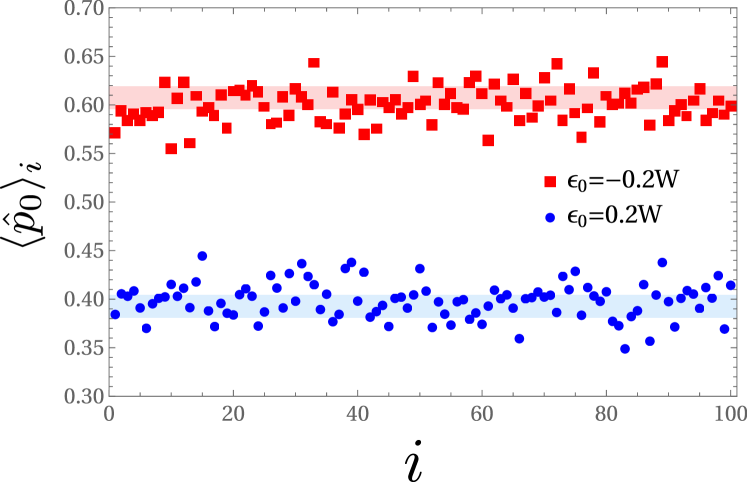
Figure 3: The system occupancies $\langle\hat{p}_{0}\rangle_{i}$ for $M=100$ individual random eigenstates $|E_{i},N_{i}\rangle$ for $\epsilon_{0}=0.2W$ (blue dots) and $\epsilon_{0}=-0.2W$ (red squares). The blue- and red-shaded regions denote the range of allowed equilibrium occupancies for $\epsilon_{0}=0.2W$ and $\epsilon_{0}=-0.2W$, respectively. Parameters: $\Gamma=0.2W$, $K=300$.

In Fig. 3 we present the system population $\langle\hat{p}_{0}\rangle_{i}$ calculated for 100 randomly generated eigenstates $|E_{i},N_{i}\rangle$ for $K=300$, $\Gamma=0.2W$ corresponding to the delocalized phase, and two different system level energies: $\epsilon_{0}=0.2W$ (blue dots) and the $\epsilon_{0}=-0.2W$ (red squares). Correspondingly, the shaded regions denote the range of allowed equilibrium occupancies of the system for the considered temperature window $T\in[0.4W,0.5W]$ and the system energy $\epsilon_{0}=0.2W$ (blue-shaded region) or $\epsilon_{0}=-0.2W$ (red-shaded region). As one can observe, the system occupancies for individual eigenstates tend to be distributed in or near the corresponding shaded regions. Thus, the system occupancy tends to thermalize.

Figure 4: The occupancies of the bath level $k=210$ for $M=100$ individual random eigenstates $|E_{i},N_{i}\rangle$ (blue dots). The blue-shaded region denotes the range of allowed equilibrium occupancies. Parameters: $\epsilon_{0}=0.2W$, $\Gamma=0.2W$, $K=300$.

As already suggested by the results on localization properties, a very different behavior is observed for occupancies of the bath levels. This is illustrated in Fig. 4 for $\epsilon_{0}=0.2W$ and the level $k=210$, whose energy $\epsilon_{k}$ is closest to $\epsilon_{0}$. As shown, now the level occupancies tend to be distributed around four different bands rather than around the blue-shaded region corresponding to the range of allowed equilibrium occupancies. This implies that, in contrast to the system, the local observables of the bath do not thermalize.

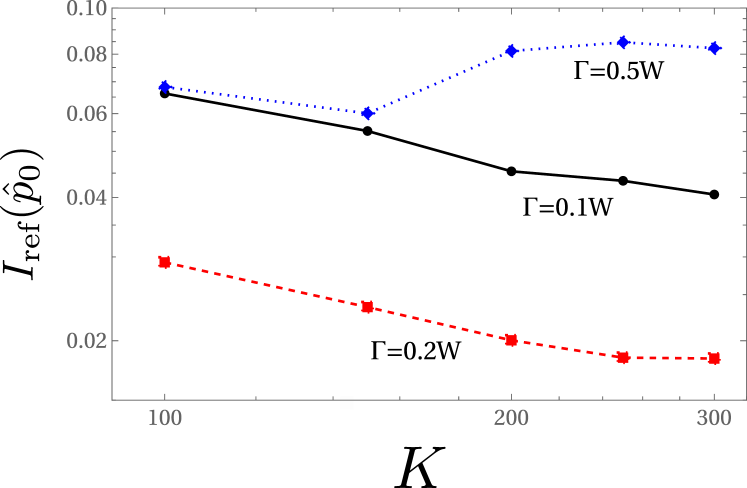
Figure 5: Scaling of the indicator of eigenstate thermalization $I_{\text{ref}}(\hat{p}_{0})$ with the number of levels $K$ for different values of the coupling strength $\Gamma$, evaluated for $M=100$ randomly generated eigenstates. The results are represented by dots, and lines are added for eye guidance. Parameters: $\epsilon_{0}=0.2W$.

To illustrate the system thermalization further, we calculate a modified indicator of eigenstate thermalization defined as

$$I_{\text{ref}}(\hat{p}_{0})\equiv\sqrt{\frac{1}{M}\sum_{i=1}^{M}(\langle\hat{p}_{0}\rangle_{i}-\langle\hat{p}_{0}\rangle_{\text{gc},i})^{2}},$$ (29)

where $M$ is the number of considered eigenstates, and $\langle\hat{p}_{0}\rangle_{\text{gc},i}=\text{Tr}(\rho_{\text{gc},i}\hat{p}_{0})$. It measures the deviation of the system occupancy evaluated for individual eigenstates and reference grand canonical states. In Fig. 5 we present the scaling of this quantity with $K$ (in the log-log scale) for different values of the coupling strength $\Gamma$. For $\Gamma=0.1W$ and $\Gamma=0.2W$, corresponding to the delocalized phase, the indicator decreases with $K$ approximately as $1/\sqrt{K}$. Some deviations from this behavior are related to the finite size of the sample $M=100$. This implies that the system occupancy tends to thermalize in the thermodynamic limit $K\rightarrow\infty$. We note that the polynomial decrease of the indicator of eigenstate thermalization is characteristic for weak ETH, whereas for strong ETH it is rather exponential [42, 54, 49, 50].

In contrast, for $\Gamma=0.5W$, corresponding to the localized phase, the indicator tends to saturate at a constant value independent of $K$, implying the absence of thermalization. We note that a similar suppression of thermalization by localization was previously observed for noninteracting fermionic lattice models [48], as well as interacting nonintegrable systems, where it is referred to as the many-body localization [64, 65, 66]. This confirms our previous theoretical reasoning based on the analysis of the inverse participation ratio $\text{IPR}_{0}$.

V Thermalization after quench

Let us now consider a dynamical scenario in which the system-bath setup is initialized in the eigenstate of the Hamiltonian $\hat{H}$, and then the Hamiltonian is quenched in the moment $t=0$ to a new form $\hat{H}^{\prime}$. Specifically, we consider a quench of the system energy level from $\epsilon_{0}$ to $\epsilon_{0}^{\prime}$, leaving the other parameters unchanged. Following Sec. II, we work within the Heisenberg picture, considering the evolution of the time-dependent observable $\hat{p}_{k}(t)$. Using Eq. (11), the evolution of the occupancy of level $k$ can be expressed as

$$\langle\hat{p}_{k}(t)\rangle=\sum_{l=0}^{K-1}|a_{kl}(t)|^{2}\langle\hat{n}_{l}\rangle.$$ (30)

The equation is analogous to Eq. (21) used in the time-independent case. Therefore, we may use the same arguments as in Sec. IV.1 to obtain the bound for the indicator of the eigenstate thermalization:

$$I_{\text{mc}}[\hat{p}_{k}(t)]\lessapprox\frac{1}{2}\sqrt{\text{IPR}_{k}(t)},$$ (31)

where

$$\text{IPR}_{k}(t)\equiv\sum_{l=0}^{K-1}|a_{kl}(t)|^{4}$$ (32)

is the time-dependent inverse participation ratio.

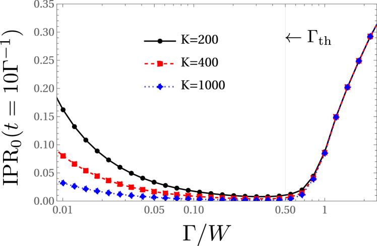
Figure 6: The time-dependent inverse participation ratio $\text{IPR}_{0}(t)$ as a function of the coupling strength $\Gamma$ for a fixed time $t=10\Gamma^{-1}$ and different number of levels $K$. Parameters: $\epsilon_{0}=0.2W$, $\epsilon_{0}^{\prime}=-0.2W$.

We now consider the case when the system energy is quenched from $\epsilon_{0}=0.2W$ to $\epsilon_{0}^{\prime}=-0.2W$ at time $t=0$. In Fig. 6 we present the inverse participation ratio $\text{IPR}_{0}(t)$ as a function of $\Gamma$ for a fixed time $t=10\Gamma^{-1}$. It exhibits a qualitatively similar behavior to the time-independent inverse participation ratio (corresponding to $t=0$) presented in Fig. 2. A notable difference is that the localization threshold $\Gamma_{\text{th}}$ is now shifted to a larger value of about $W/2$.

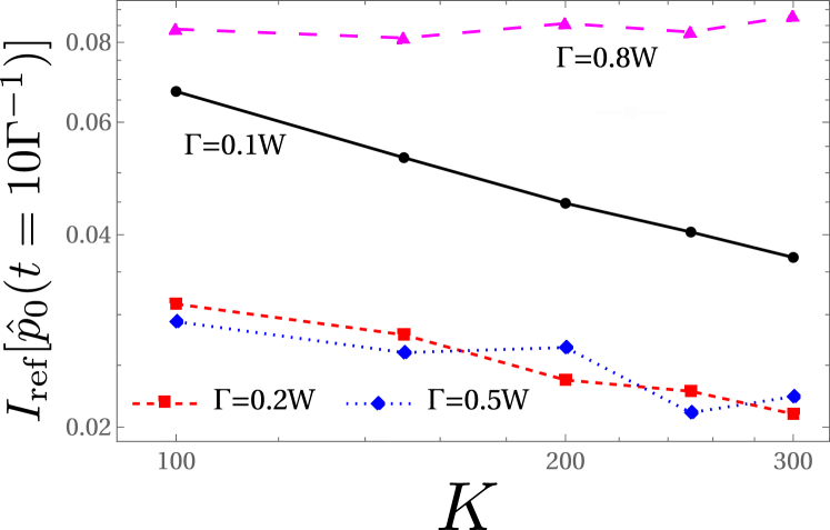
Figure 7: Scaling of the indicator of eigenstate thermalization $I_{\text{ref}}[\hat{p}_{0}(t)]$ with the number of level $K$ for different values of the coupling strength $\Gamma$, evaluated for $M=100$ randomly generated eigenstates and a fixed time $t=10\Gamma^{-1}$. The results are represented by dots, and lines are added for eye guidance. Parameters: $\epsilon_{0}=0.2W$, $\epsilon_{0}^{\prime}=-0.2W$.

In Fig. 7 we present the scaling of the modified indicator of eigenstate thermalization $I_{\text{ref}}[\hat{p}_{0}(t)]$ defined in Eq. (29) for a fixed time $t=10\Gamma^{-1}$. As previously, we consider only those eigenstates, whose reference temperatures belong to the interval $[0.4W,0.5W]$. We can observe a decrease of the analyzed quantity with increasing $K$ for $\Gamma=0.1W$ and $\Gamma=0.2W$ belonging to the delocalized regime. However, a decrease is now also observed for $\Gamma=0.5W$. This is because, as shown in Fig. 6, this coupling value now corresponds to the border of the delocalized and localized phase, rather than being located within the localized phase. However, the effect of localization is clearly visible for an even larger $\Gamma=0.8W$.

Thus far, we have shown that (in the delocalized regime and for large bath sizes) the evolution of the system tends to be the same for the system-bath setup initialized in typical eigenstates of its initial Hamiltonian and in the corresponding thermal states. Now, we go a step further by noting a well-established observation of open quantum system theory [67, 68, 69, 70, 71, 72, 73]: When the system-bath setup is initialized in the thermal state of the initial Hamiltonian $\hat{H}$, and then the Hamiltonian is weakly quenched, the reduced state of the system tends to relax to the equilibrium state for the new Hamiltonian. The justification for this occurrence and its conditions are thoroughly discussed in Ref. [73]. In particular, the perturbation has to be sufficiently weak, e.g., affect only the system Hamiltonian, without changing the bath Hamiltonian (which is a scenario considered here). Thus, one may expect that the same relaxation to the equilibrium value for the new Hamiltonian would also be observed when the system-bath setup is initialized in a typical eigenstate of its initial Hamiltonian $\hat{H}$.

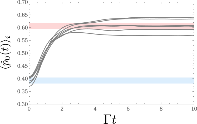
Figure 8: The evolution of the system occupancies $\langle\hat{p}_{0}(t)\rangle_{i}$ for six individual random eigenstates $|E_{i},N_{i}\rangle$ (gray solid lines). Blue- and red-shaded regions denote the range of allowed equilibrium occupancies of the system for the initial and the final Hamiltonian, respectively. Parameters: $\epsilon_{0}=0.2W$, $\epsilon_{0}^{\prime}=-0.2W$, $\Gamma=0.2W$, $K=300$.

To demonstrate that, in Fig. 8 we show the dynamics of the system occupancy $\langle\hat{p}_{0}(t)\rangle_{i}$ for a system-bath setup initialized in six different randomly generated eigenstates of the initial Hamiltonian. We choose $\Gamma=0.2W$ corresponding to the delocalized regime. It can be seen that initially the populations are distributed near the blue-shaded region, which corresponds to the range of allowed equilibrium occupancies of the system for the initial Hamiltonian $\hat{H}$. Then, the populations evolve so that after a certain time of the order of $\Gamma^{-1}$ the populations focus around the red-shaded region, which corresponds to the range of allowed equilibrium occupancies for the final Hamiltonian $\hat{H}^{\prime}$. Thus, the Hamiltonian quench indeed drives the system to thermalize with respect to the final Hamiltonian.

The occurrence of thermalization in the considered scenario is quite remarkable, as integrable models usually do not thermalize after quench, even when they exhibit thermalization of static observables [42, 43]. As already mentioned, the presence of thermalization in our case is related to the fact that we quench only the system Hamiltonian, leaving the bath Hamiltonian unchanged. Thus, the considered quench is only a small perturbation to the total system-bath Hamiltonian. Thermalization would not be observed for stronger perturbations, involving also the bath Hamiltonian. This does not invalidate the significance of our result, as quenches affecting only the system Hamiltonian are very relevant from the experimental point of view. For example, they correspond to typical experiments in the field of nanothermodynamics, performed on quantum dots or single-electron transistors attached to electrodes [74, 75, 76, 77].

VI Thermalization induced by bath eigenstates

So far we have focused on the case where the system-bath setup was initialized in the eigenstate of the total Hamiltonian $\hat{H}$. Let us now consider another case, where the initial state of the system is arbitrary, while the bath is initialized in the eigenstate of its Hamiltonian

$$\hat{H}_{B}=\sum_{k=1}^{K-1}\epsilon_{k}c_{k}^{\dagger}c_{k}.$$ (33)

Such eigenstates are then denoted as $|E^{B}_{i},N^{B}_{i}\rangle$. The initial state of the system-bath setup reads then

$$\rho_{i}(0)=\rho_{S}(0)\otimes|E^{B}_{i},N^{B}_{i}\rangle\langle E^{B}_{i},N^{B}_{i}|,$$ (34)

where $\rho_{S}(0)$ is the initial state of the system. A similar scenario, in which the baths were initialized in pure states sampled from the grand canonical ensemble, was recently investigated in Ref. [53].

Let us also define the initial state

$$\rho_{\text{mc}}(0)\equiv\rho_{S}(0)\otimes\rho_{\text{mc}}^{B},$$ (35)

which corresponds to the initial microcanonical state of the bath. Here $\rho_{\text{mc}}^{B}$ is defined via the right-hand-side of Eq. (14) with $|E_{i},N_{i}\rangle$ replaced by $|E^{B}_{i},N^{B}_{i}\rangle$. We now compare the dynamics of the system occupancy generated by single eigenstates and the microcanonical state. As previously, we work in the Heisenberg picture. The dynamics of the system occupancy is described via Eq. (30). The quench of the Hamiltonian now corresponds to the switching-on of the tunnel coupling $\Gamma$ at the time $t=0$. Since the system and the bath are initially uncoupled, we have $c_{k}=d_{k}$, $\hat{p}_{k}=\hat{n}_{k}$ and $a_{kl}=\delta_{kl}$.

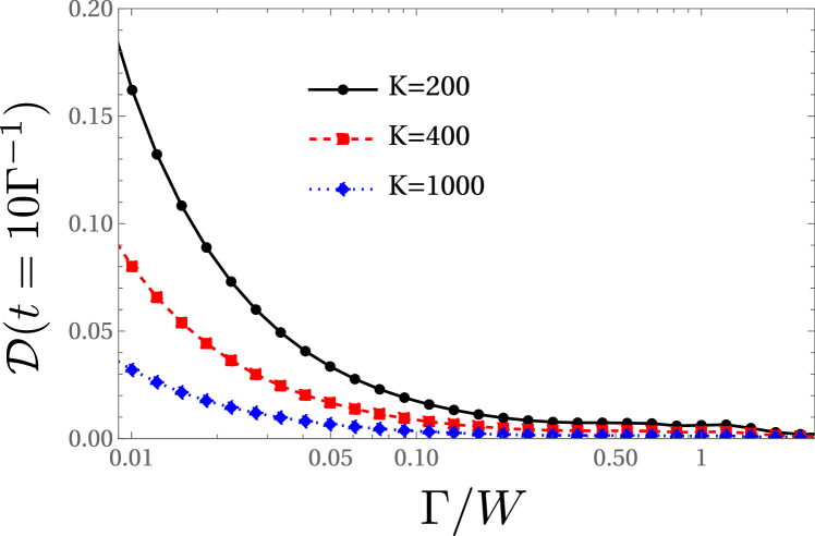
Figure 9: The localization coefficient $\mathcal{D}(t)$ as a function of the coupling strength $\Gamma$ for a fixed time $t=10\Gamma^{-1}$ and different number of levels $K$. Parameters: $\epsilon_{0}=-0.2W$.

Let us now consider the indicator of eigenstate thermalization defined in Eq. (17), where we now take $\langle\hat{A}\rangle_{i}=\text{Tr}[\rho_{i}(0)\hat{A}]$ and $\langle\hat{A}\rangle_{\text{mc}}=\text{Tr}[\rho_{\text{mc}}(0)\hat{A}]$. Using the same arguments as before, it can be bounded as

$$I_{\text{mc}}[\hat{p}_{0}(t)]\lessapprox\frac{1}{2}\sqrt{\mathcal{D}(t)},$$ (36)

where

$$\mathcal{D}(t)\equiv\text{IPR}_{0}(t)-|a_{00}(t)|^{4}=\sum_{l=1}^{K-1}|a_{0l}(t)|^{4}$$ (37)

is the localization coefficient. It corresponds to the previously defined time-dependent inverse participation ratio $\text{IPR}_{0}(t)$ with an excluded element $|a_{00}(t)|^{4}$; this is because the initial system occupancy is now the same for the states $\rho_{i}(0)$ and $\rho_{\text{mc}}(0)$. In Fig. 9 we plot this quantity as a function of $\Gamma$ for a fixed time $t=10\Gamma^{-1}$. One may observe that, in contrast to the inverse participation ratio, the localization coefficient does not imply localization for a large $\Gamma$. Therefore, the thermal behavior of the system occupancy can be expected regardless of coupling strength $\Gamma$. We note that the formation of bound states for large $\Gamma$ still manifests itself in the nonvanishing long-time value of the element $|a_{00}(t)|^{4}$, which corresponds to the long-time memory of the system about its initial state. However, this element does not contribute to $\mathcal{D}(t)$.

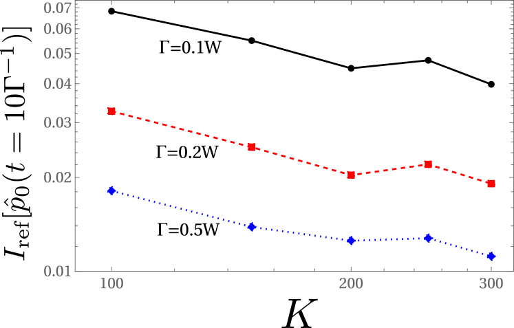
Figure 10: Scaling of the indicator of eigenstate thermalization $I_{\text{ref}}[\hat{p}_{0}(t)]$ with the number of level $K$ for different values of the coupling strength $\Gamma$, evaluated for $M=100$ randomly generated bath eigenstates and a fixed time $t=10\Gamma^{-1}$. The results are represented by dots, and lines are added for eye guidance. Parameters: $\langle\hat{p}(0)\rangle=0$, $\epsilon_{0}=-0.2W$.

Let us now analyze the modified indicator of eigenstate thermalization defined via Eq. (29). The system occupancy for the reference thermal state is now defined as $\langle\hat{p}_{0}(t)\rangle_{\text{gc},i}\equiv\text{Tr}[\rho_{\text{gc},i}(0)\hat{p}_{0}(t)]$, where $\rho_{\text{gc},i}(0)\equiv\rho_{S}(0)\otimes\rho^{B}_{\text{gc},i}$ and $\rho^{B}_{\text{gc},i}$ is the reference grand canonical state of the bath with the same energy and particle number as the considered eigenstate. We further focus on the case where the system is initially empty $(\langle\hat{p}(0)\rangle=0)$ and the bath is initially half-filled [$N_{i}^{B}=(K-1)/2$]. As before, we consider only those eigenstates of the bath, whose reference temperatures $T_{i}$ belong to the interval $[0.4W,0.5W]$. The scaling of the analyzed quantity with $K$ for different coupling strengths $\Gamma$ is presented in Fig. 10; here we use the same random eigenstates for all values of $\Gamma$. As in the cases considered above, it decreases with the system size (with certain statistical errors due to the finite sample size), implying thermalization in the thermodynamic limit $K\rightarrow\infty$. As suggested by Fig. 9, this is also observed for large values of $\Gamma$, since the localization now does not suppress the thermalization.

Figure 11: The evolution of the system occupancies $\langle\hat{p}_{0}(t)\rangle_{i}$ for six individual initial random bath eigenstates $|E_{i}^{B},N_{i}^{B}\rangle$ (gray solid lines) for an intermediate system-bath coupling $\Gamma=0.2W$. The red-shaded region denotes the range of allowed equilibrium occupancies. Parameters: $\langle\hat{p}(0)\rangle=0$, $\epsilon_{0}=-0.2W$, $K=301$.

Finally, as in the previous section, we analyze the evolution of the system occupancy to establish whether it relaxes to the equilibrium state for the total Hamiltonian. In Fig. 11 we show dynamics of the system occupancy for the bath initialized in six different random eigenstates for an intermediate system-bath coupling $\Gamma=0.2W$. As before, the red-shaded region denotes the range of allowed equilibrium system occupancies of the system for chosen Hamiltonian parameters and temperatures belonging to the considered window. Analogously to the case of Hamiltonian quench, after a certain relaxation time, the system occupancies focus around the red-shaded region, which witnesses the system relaxation to equilibrium.

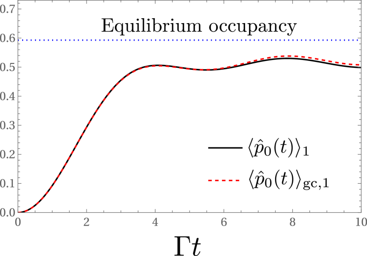
Figure 12: The evolution of the system occupancies for an initial bath eigenstate $|E_{1}^{B},N_{1}^{B}\rangle$ (black solid line) and the reference grand canonical state (red solid line) for a strong system-bath coupling $\Gamma=0.8W$. The blue dotted line denotes the equilibrium occupancy evaluated for the reference temperature $T_{1}$ and the chemical potential $\mu_{1}$. Other parameters as in Fig. 11.

To account for the effect of localization in the considered scenario, in Fig. 12 we present the evolution of the system occupancy for a large coupling strength $\Gamma=0.8W$. We focus on the evolution for a single initial state $\rho_{1}(0)$ (black solid line). It is compared with the results for a reference grand canonical state (red dashed line). The blue dotted line denotes the equilibrium occupancy calculated for the temperature $T_{1}$ and the chemical potential $\mu_{1}=0$ of the reference grand canonical state. We can see that now the system occupancy does not converge to its equilibrium value. This is characteristic for systems with bound states due to the long-time memory of the system about its initial state, which is encoded in the amplitude $|a_{00}(t)|^{2}$ [60, 61, 62, 63]. However, the system behavior is still thermal in the sense that the evolution of the system occupancy induced by the initial eigenstate of the bath and the reference thermal state is approximately the same.

VII Conclusions

We investigated the behavior of observables for individual eigenstates of a fully integrable noninteracting resonant level model. We have shown that typical eigenstates exhibit thermalization of the system occupancy, that is, the occupancy tends to have the same value as for the thermal state with the same energy and particle number as the considered eigenstate. Thermalization is related to delocalization of the single-particle state, corresponding to the occupied state of the system, over many single-particle eigenstates of the system-bath Hamiltonian. As a consequence, the system occupancy can be expressed as a weighted average of occupancies of the single-particle eigenstates. As shown by Khinchin in the context of classical systems [29], such averages of many independent degrees of freedom tend to thermalize in the thermodynamic limit due to the law of large numbers, independent of details of the system dynamics. We further show that the system thermalization becomes suppressed when the occupied state of the system becomes strongly localized in a few single-particle eigenstates due to formation of the bound states for a strong system-bath coupling. Furthermore, thermalization is not observed for the occupancies of the bath levels, which are always strongly localized.

We further went beyond the static scenario to consider the case where the system Hamiltonian is quenched at some moment of time. We have shown that after such a quench, the system occupancy tends to relax to the thermal value corresponding to a new Hamiltonian. This is remarkable, as integrable systems generally do not thermalize after quench, even when they exhibit thermalization of static observables [42, 43]. The presence of thermalization in our case is related to the fact that the quench involves only parameters of the system and not of the bath. Therefore, it only weakly perturbs the total system-bath Hamiltonian. Such quenches that involve only the system Hamiltonian are common in experiments on open quantum systems [74, 75, 76, 77].

Finally, we considered the case where the initial state of the system is arbitrary, while the bath is initialized in an eigenstate of its Hamiltonian. Then, for typical eigenstates, we observed the same thermalization behavior of the system as for baths initialized in thermal states with the same energy and particle number. While we focused on a system coupled to a single bath, this approach can easily be generalized to a multiple-bath scenario. In such a case, we may expect the emergence of nonequilibrium steady states, as previously observed for baths obeying ETH [23, 24] or initialized in pure states sampled from the grand canonical ensemble [53].

The paper contributes to the ongoing debate on whether nonintegrability should be regarded as a requirement for thermalization [25, 26, 37, 28, 31, 33, 32]. It is known that integrable systems do not exhibit thermalization of all observables in all physical scenarios [42, 43, 48, 18, 19]. In the considered system, this is illustrated by the lack of thermalization of bath level occupancies, or suppression of the system thermalization in the localized regime. The system will also not thermalize after the quench of the bath Hamiltonian. Nevertheless, the paper supports the conclusion of Refs. [31, 28, 53, 33, 32] that integrable systems can still exhibit a genuine thermal behavior of physically meaningful quantities in many physically relevant scenarios. Therefore, nonintegrability, chaos, and ETH should not be regarded (as sometimes done [25, 16]) as the sole mechanism to explain the origin of thermalization. Rather, there is value in using different complementary approaches (including arguments based on the typicality of states and observables) to get a complete picture of the emergence of thermodynamic behavior.

References

- Lebowitz and Penrose [1973] J. L. Lebowitz and O. Penrose, Modern ergodic theory, Physics Today 26, 23 (1973).
- Sinai [1963] Y. G. Sinai, On the foundations of the ergodic hypothesis for a dynamical system of statistical mechanics, Sov. Math., Dokl. 4, 1818 (1963).
- Sinai [1970] Y. G. Sinai, Dynamical systems with elastic reflections, Russ. Math. Surv. 25, 137 (1970).
- Bunimovich [1979] L. A. Bunimovich, On the ergodic properties of nowhere dispersing billiards, Commun. Math. Phys. 65, 295 (1979).
- Simányi [2004] N. Simányi, Proof of the Ergodic Hypothesis for Typical Hard Ball Systems, Ann. Henri Poincaré 5, 203 (2004).
- Gaspard [1998] P. Gaspard, Chaos, Scattering and Statistical Mechanics (Cambridge University Press, Cambridge, 1998).
- Dorfman [1999] J. Dorfman, An Introduction to Chaos in Nonequilibrium Statistical Mechanics, Cambridge Lecture Notes in Physics (Cambridge University Press, Cambridge, 1999).
- Kolmogorov [1954] A. N. Kolmogorov, On conservation of conditionally periodic motions for a small change in Hamilton’s function, Dokl. Akad. Nauk SSSR 98, 527 (1954).
- Arnol’d [1963] V. I. Arnol’d, Proof of a theorem of A. N. Kolmogorov on the preservation of conditionally-periodic motions under small perturbations of the Hamiltonian, Russ. Math. Surv. 18, 9 (1963).
- Moser [1962] J. K. Moser, On invariant curves of area-preserving mapping of an annulus, Nachr. Akad. Wiss. Göttingen Math.-Phys. Kl. II 1962, 1 (1962).
- Fermi et al. [1955] E. Fermi, P. Pasta, and S. Ulam, Studies of Nonlinear Problems, Los Alamos National Laboratory, Document LA-1940 (1955).
- Dauxois [2008] T. Dauxois, Fermi, Pasta, Ulam, and a mysterious lady, Physics Today 61, 55 (2008).
- Gogolin and Eisert [2016] C. Gogolin and J. Eisert, Equilibration, thermalisation, and the emergence of statistical mechanics in closed quantum systems, Rep. Prog. Phys. 79, 056001 (2016).
- Deutsch [1991] J. M. Deutsch, Quantum statistical mechanics in a closed system, Phys. Rev. A 43, 2046 (1991).
- Srednicki [1994] M. Srednicki, Chaos and quantum thermalization, Phys. Rev. E 50, 888 (1994).
- Deutsch [2018] J. M. Deutsch, Eigenstate thermalization hypothesis, Rep. Prog. Phys. 81, 082001 (2018).
- D’Alessio et al. [2016] L. D’Alessio, Y. Kafri, A. Polkovnikov, and M. Rigol, From quantum chaos and eigenstate thermalization to statistical mechanics and thermodynamics, Adv. Phys. 65, 239 (2016).
- Rigol et al. [2007] M. Rigol, V. Dunjko, V. Yurovsky, and M. Olshanii, Relaxation in a Completely Integrable Many-Body Quantum System: An Ab Initio Study of the Dynamics of the Highly Excited States of 1D Lattice Hard-Core Bosons, Phys. Rev. Lett. 98, 050405 (2007).
- Cassidy et al. [2011] A. C. Cassidy, C. W. Clark, and M. Rigol, Generalized Thermalization in an Integrable Lattice System, Phys. Rev. Lett. 106, 140405 (2011).
- Ilievski et al. [2015] E. Ilievski, J. De Nardis, B. Wouters, J.-S. Caux, F. H. Essler, and T. Prosen, Complete Generalized Gibbs Ensembles in an Interacting Theory, Phys. Rev. Lett. 115, 157201 (2015).
- Polkovnikov et al. [2011] A. Polkovnikov, K. Sengupta, A. Silva, and M. Vengalattore, Colloquium: Nonequilibrium dynamics of closed interacting quantum systems, Rev. Mod. Phys. 83, 863 (2011).
- Iyoda et al. [2017] E. Iyoda, K. Kaneko, and T. Sagawa, Fluctuation Theorem for Many-Body Pure Quantum States, Phys. Rev. Lett. 119, 100601 (2017).
- Xu et al. [2022] X. Xu, C. Guo, and D. Poletti, Typicality of nonequilibrium quasi-steady currents, Phys. Rev. A 105, L040203 (2022).
- Xu et al. [2023] X. Xu, C. Guo, and D. Poletti, Emergence of steady currents due to strong prethermalization, Phys. Rev. A 107, 022220 (2023).
- De Palma et al. [2015] G. De Palma, A. Serafini, V. Giovannetti, and M. Cramer, Necessity of Eigenstate Thermalization, Phys. Rev. Lett. 115, 220401 (2015).
- Bartsch and Gemmer [2017] C. Bartsch and J. Gemmer, Necessity of eigenstate thermalisation for equilibration towards unique expectation values when starting from generic initial states, Europhys. Lett. 118, 10006 (2017).
- Lebowitz [1993] J. L. Lebowitz, Macroscopic laws, microscopic dynamics, time’s arrow and Boltzmann’s entropy, Physica A 194, 1 (1993).
- Chakraborti et al. [2022] S. Chakraborti, A. Dhar, S. Goldstein, A. Kundu, and J. L. Lebowitz, Entropy growth during free expansion of an ideal gas, J. Phys. A: Math. Theor. 55, 394002 (2022).
- Khinchin [1949] A. I. Khinchin, Mathematical Foundations Of Statistical Mechanics (Dover Publications, New York, 1949).
- Mazur and Van der Linden [1963] P. Mazur and J. Van der Linden, Asymptotic Form of the Structure Function for Real Systems, J. Math. Phys. 4, 271 (1963).
- Baldovin et al. [2021] M. Baldovin, A. Vulpiani, and G. Gradenigo, Statistical mechanics of an integrable system, J. Stat. Phys. 183, 41 (2021).
- Cocciaglia et al. [2022] N. Cocciaglia, A. Vulpiani, and G. Gradenigo, Thermalization without chaos in harmonic systems, Physica A 601, 127581 (2022).
- Baldovin et al. [2023] M. Baldovin, R. Marino, and A. Vulpiani, Ergodic observables in non-ergodic systems: the example of the harmonic chain, Physica A 630, 129273 (2023).
- von Neumann [2010] J. von Neumann, Proof of the ergodic theorem and the H-theorem in quantum mechanics, Eur. Phys. J. H 35, 201 (2010).
- Goldstein et al. [2010] S. Goldstein, J. L. Lebowitz, C. Mastrodonato, R. Tumulka, and N. Zanghi, Normal typicality and von Neumann’s quantum ergodic theorem, Proc. R. Soc. A 466, 3203 (2010).
- Reimann [2015] P. Reimann, Generalization of von Neumann’s Approach to Thermalization, Phys. Rev. Lett. 115, 010403 (2015).
- Rigol and Srednicki [2012] M. Rigol and M. Srednicki, Alternatives to Eigenstate Thermalization, Phys. Rev. Lett. 108, 110601 (2012).
- Tasaki [1998] H. Tasaki, From Quantum Dynamics to the Canonical Distribution: General Picture and a Rigorous Example, Phys. Rev. Lett. 80, 1373 (1998).
- Gemmer and Mahler [2003] J. Gemmer and G. Mahler, Distribution of local entropy in the Hilbert space of bi-partite quantum systems: origin of Jaynes’ principle, Eur. Phys. J. B 31, 249 (2003).
- Goldstein et al. [2006] S. Goldstein, J. L. Lebowitz, R. Tumulka, and N. Zanghì, Canonical Typicality, Phys. Rev. Lett. 96, 050403 (2006).
- Popescu et al. [2006] S. Popescu, A. J. Short, and A. Winter, Entanglement and the foundations of statistical mechanics, Nat. Phys. 2, 754 (2006).
- Biroli et al. [2010] G. Biroli, C. Kollath, and A. M. Läuchli, Effect of Rare Fluctuations on the Thermalization of Isolated Quantum Systems, Phys. Rev. Lett. 105, 250401 (2010).
- Nandy et al. [2016] S. Nandy, A. Sen, A. Das, and A. Dhar, Eigenstate Gibbs ensemble in integrable quantum systems, Phys. Rev. B 94, 245131 (2016).
- Mori and Shiraishi [2017] T. Mori and N. Shiraishi, Thermalization without eigenstate thermalization hypothesis after a quantum quench, Phys. Rev. E 96, 022153 (2017).
- [45] A. W. Harrow and Y. Huang, Thermalization without eigenstate thermalization, arXiv:2209.09826 .
- Magán [2016] J. M. Magán, Random Free Fermions: An Analytical Example of Eigenstate Thermalization, Phys. Rev. Lett. 116, 030401 (2016).
- Lai and Yang [2015] H.-H. Lai and K. Yang, Entanglement entropy scaling laws and eigenstate typicality in free fermion systems, Phys. Rev. B 91, 081110(R) (2015).
- Li et al. [2016] X. Li, J. Pixley, D.-L. Deng, S. Ganeshan, and S. D. Sarma, Quantum nonergodicity and fermion localization in a system with a single-particle mobility edge, Phys. Rev. B 93, 184204 (2016).
- Łydżba et al. [2023] P. Łydżba, M. Mierzejewski, M. Rigol, and L. Vidmar, Generalized Thermalization in Quantum-Chaotic Quadratic Hamiltonians, Phys. Rev. Lett. 131, 060401 (2023).
- [50] P. Łydżba, R. Świętek, M. Mierzejewski, M. Rigol, and L. Vidmar, Normal weak eigenstate thermalization, arXiv:2404.02199 .
- [51] N. Shiraishi and H. Tasaki, Nature abhors a vacuum: A simple rigorous example of thermalization in an isolated macroscopic quantum system, arXiv:2310.18880 .
- [52] H. Tasaki, Macroscopic irreversibility in quantum systems: ETH and equilibration in a free fermion chain, arXiv:2401.15263 .
- Usui et al. [2024] A. Usui, K. Ptaszyński, M. Esposito, and P. Strasberg, Microscopic contributions to the entropy production at all times: from nonequilibrium steady states to global thermalization, New J. Phys. 26, 023049 (2024).
- Mori et al. [2018] T. Mori, T. N. Ikeda, E. Kaminishi, and M. Ueda, Thermalization and prethermalization in isolated quantum systems: a theoretical overview, J. Phys. B: At. Mol. Opt. Phys 51, 112001 (2018).
- Kramer and MacKinnon [1993] B. Kramer and A. MacKinnon, Localization: theory and experiment, Rep. Prog. Phys. 56, 1469 (1993).
- Linden et al. [2009] N. Linden, S. Popescu, A. J. Short, and A. Winter, Quantum mechanical evolution towards thermal equilibrium, Phys. Rev. E 79, 061103 (2009).
- Short [2011] A. J. Short, Equilibration of quantum systems and subsystems, New J. Phys. 13, 053009 (2011).
- Short and Farrelly [2012] A. J. Short and T. C. Farrelly, Quantum equilibration in finite time, New J. Phys. 14, 013063 (2012).
- Esposito and Gaspard [2003] M. Esposito and P. Gaspard, Spin relaxation in a complex environment, Phys. Rev. E 68, 066113 (2003).
- Cai et al. [2014] C.-Y. Cai, L.-P. Yang, C. Sun, et al., Threshold for nonthermal stabilization of open quantum systems, Phys. Rev. A 89, 012128 (2014).
- Xiong et al. [2015] H.-N. Xiong, P.-Y. Lo, W.-M. Zhang, D. H. Feng, and F. Nori, Non-Markovian Complexity in the Quantum-to-Classical Transition, Sci. Rep. 5, 13353 (2015).
- Yang et al. [2015] P.-Y. Yang, C.-Y. Lin, and W.-M. Zhang, Master equation approach to transient quantum transport in nanostructures incorporating initial correlations, Phys. Rev. B 92, 165403 (2015).
- Jussiau et al. [2019] É. Jussiau, M. Hasegawa, and R. S. Whitney, Signature of the transition to a bound state in thermoelectric quantum transport, Phys. Rev. B 100, 115411 (2019).
- Oganesyan and Huse [2007] V. Oganesyan and D. A. Huse, Localization of interacting fermions at high temperature, Phys. Rev. B 75, 155111 (2007).
- Žnidarič et al. [2008] M. Žnidarič, T. Prosen, and P. Prelovšek, Many-body localization in the Heisenberg magnet in a random field, Phys. Rev. B 77, 064426 (2008).
- Abanin et al. [2019] D. A. Abanin, E. Altman, I. Bloch, and M. Serbyn, Colloquium: Many-body localization, thermalization, and entanglement, Rev. Mod. Phys. 91, 021001 (2019).
- Jakšić and Pillet [1996] V. Jakšić and C.-A. Pillet, On a model for quantum friction III. Ergodic properties of the spin-boson system, Commun. Math. Phys. 178, 627 (1996).
- Bach et al. [2000] V. Bach, J. Fröhlich, and I. M. Sigal, Return to equilibrium, J. Math. Phys. 41, 3985 (2000).
- Merkli [2001] M. Merkli, Positive commutators in non-equilibrium quantum statistical mechanics, Commun. Math. Phys. 223, 327 (2001).
- Fröhlich and Merkli [2004] J. Fröhlich and M. Merkli, Another return of “return to equilibrium”, Commun. Math. Phys. 251, 235 (2004).
- Merkli et al. [2007] M. Merkli, I. M. Sigal, and G. P. Berman, Decoherence and Thermalization, Phys. Rev. Lett. 98, 130401 (2007).
- Merkli et al. [2008] M. Merkli, I. Sigal, and G. Berman, Resonance theory of decoherence and thermalization, Ann. Phys. (N.Y.) 323, 373 (2008).
- Trushechkin et al. [2022] A. S. Trushechkin, M. Merkli, J. D. Cresser, and J. Anders, Open quantum system dynamics and the mean force Gibbs state, AVS Quantum Sci. 4, 012301 (2022).
- Koski et al. [2013] J. V. Koski, T. Sagawa, O. P. Saira, Y. Yoon, A. Kutvonen, P. Solinas, M. Möttönen, T. Ala-Nissila, and J. P. Pekola, Distribution of entropy production in a single-electron box, Nat. Phys. 9, 644 (2013).
- Koski et al. [2014] J. V. Koski, V. F. Maisi, J. P. Pekola, and D. V. Averin, Experimental realization of a Szilard engine with a single electron, Proc. Natl. Acad. Sci. U.S.A. 111, 13786 (2014).
- Maillet et al. [2019] O. Maillet, P. A. Erdman, V. Cavina, B. Bhandari, E. T. Mannila, J. T. Peltonen, A. Mari, F. Taddei, C. Jarzynski, V. Giovannetti, et al., Optimal Probabilistic Work Extraction beyond the Free Energy Difference with a Single-Electron Device, Phys. Rev. Lett. 122, 150604 (2019).
- Scandi et al. [2022] M. Scandi, D. Barker, S. Lehmann, K. A. Dick, V. F. Maisi, and M. Perarnau-Llobet, Minimally Dissipative Information Erasure in a Quantum Dot via Thermodynamic Length, Phys. Rev. Lett. 129, 270601 (2022).