Circular Distribution of Agents using
Convex Layers
Abstract
This paper considers the problem of conflict-free distribution of agents on a circular periphery encompassing all agents. The two key elements of the proposed policy include the construction of a set of convex layers (nested convex polygons) using the initial positions of the agents, and a novel search space region for each of the agents. The search space for an agent on a convex layer is defined as the region enclosed between the lines passing through the agent’s position and normal to its supporting edges. Guaranteeing collision-free paths, a goal assignment policy designates a unique goal position within the search space of an agent. In contrast to the existing literature, this work presents a one-shot, collision-free solution to the circular distribution problem by utilizing only the initial positions of the agents. Illustrative examples demonstrate the effectiveness of the proposed policy.
1 Introduction
Swarm robotics and intelligence have garnered a lot of attention over the past few decades. This is primarily due to the growing advances in robotics and related fields like microelectronics and communication technology. In contrast to a single robot, swarms offer advantages in terms of cost, mobility, reliability, and ability to cover large areas. Applications like surveillance [1], search and rescue [2], payload transport [3], and crop spraying [4] desire the agents in a swarm to be spatially arranged in geometric patterns like line, wedge, circle, or polygon.
Circular formation of agents finds specific relevance in applications like target encirclement [5], ocean sampling [6], and boundary monitoring [7]. Refs. [8, 9] have proved through their algorithms that it is always possible to bring a finite number of agents arbitrarily positioned in a plane to a circular formation. A two-stage policy proposed in Refs. [10, 11] emphasizes circular formation as an intermediate configuration that can be used to eventually achieve other geometric patterns like convex and concave polygons.
Circular formation can be achieved by assigning unique goal positions for all agents on the circular boundary and then finding non-conflicting paths for the agents to move to their respective goal positions. Ref. [12] proposed a strategy to assign goals to multiple agents wherein the agents move radially towards the circumference of a circle that encompasses all agents. That approach, however, fails to offer conflict-free goal assignment for agents lying on the same radial line. Another radial goal assignment policy is considered by Ref. [13] wherein the agents use Sense-Process-Act cycles at each time step and switch their goal positions if a collision with another agent is detected. In conjunction with the radial goal assignment policy, Ref. [10] proposed an artificial potential function-based method to avoid collision between agents. Ref. [14] uses the velocity obstacle method to avoid inter-agent collisions as agents move to occupy predefined goal positions on a circular boundary. In Ref. [15], the circular formation strategy requires the agent closest to the circle to move along the radial line toward the circumference of the circle, while the other agents positioned on the same radial line remain stationary temporarily.
In Refs. [9, 16, 17, 18, 19], the circle formation methods essentially consider Look-Compute-Move (LCM) cycle for realizing collision avoidance among agents. Therein, the agent’s speed is commanded to be zero if a collision is detected; otherwise, the agents use a positive velocity. Further, monitoring of the agent’s configuration is required at each cycle. Ref. [20] proposed a circle formation strategy in which Voronoi diagram is constructed using the initial positions of the agents as generators. The vertex of the agent’s Voronoi cell which is closest to the circle is selected as its intermediate goal point. In that approach, the non-conflicting intermediate goal assignment relies on the unboundedness of the Voronoi cells, which may not be guaranteed as the number of agents increases. While assigning goal positions to the agents on a circular boundary, Ref. [11] considers intersecting paths as conflicts without assessing the temporal aspect of the collision possibilities. In all of the aforementioned works, partial or complete knowledge of the other agents’ positions is required at all times or at discrete time steps. This is necessary to compute input commands of the agents such that there is no inter-agent collision while they move to occupy their respective goal positions on the circle. The motivation for our work is to come up with a strategy that uses only the initial position of the agents and computes, at the initial time itself, a conflict-free goal assignment on the circular periphery.
To the best of the authors’ knowledge, none of the existing circular distribution works offer a one-shot, conflict-free goal assignment policy with constant and continuous speed for the agents. This paper presents a convex layer-based approach for driving a swarm of agents on a circular boundary. The main contributions of this paper are as follows.
-
1.
A novel angular region, called the search space, is defined for each agent in the swarm. Within this search space, a goal position is defined on the circumference of a circle that encompasses all agents.
-
2.
By virtue of the proposed angular region and the convex layer on which an agent is located, a guarantee is deduced which rules out any collision possibility among agents. Once the goal positions are assigned, the agents move directly toward their goal position along a straight line with a prescribed speed.
-
3.
The proposed policy generates one-shot conflict-free trajectories deduced for any number of agents in the swarm with arbitrary initial configuration within an encompassing circle.
The remainder of the paper is organized as follows: Section 2 contains the preliminaries necessary throughout the paper. The problem is formulated in Section 3 and the main results are presented in Section 4. Examples demonstrating the proposed policy are presented in Section 5 followed by concluding remarks in Section 6.
2 Preliminaries
2.1 Convex Hull
The convex hull for a set of points, is defined as the set of all points such that
| (1) |
where , and .
Some notable algorithms used for constructing Conv in are: Graham’s scan [21], Divide and Conquer [22], and Chan’s algorithm [23]. Graham’s scan offers low complexity and is used to generate Conv in this work.
Definition 1 ([24])
A point Conv is defined as the vertex of Conv if it cannot be expressed in the form of the convex combination of any two distinct points in Conv, that is,
| (2) |
where Conv and .
Definition 2
The supporting edges of a vertex are the edges of Conv that intersect at .
Definition 3
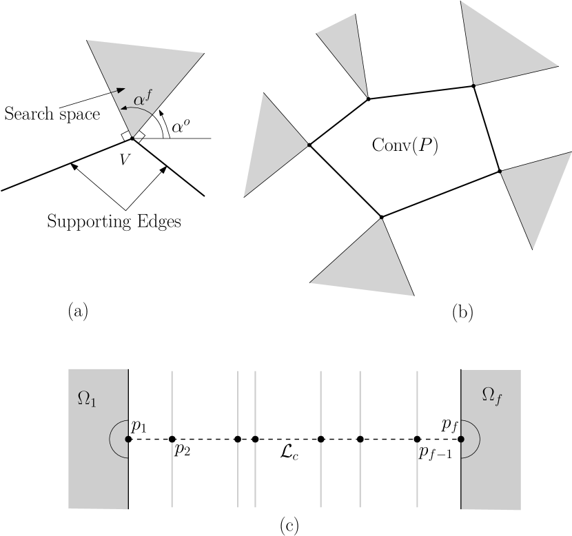
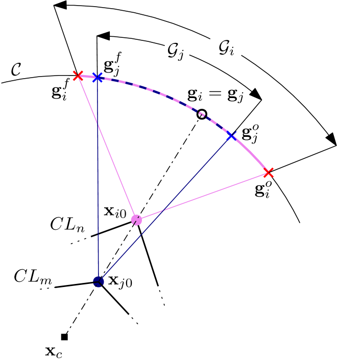
The search space for a vertex of Conv, is proposed as the angular region enclosed by the normals drawn at the supporting edges at (Fig. 1a). The search space range .
In the scenario where the points in are collinear on a line , the search space region of is the half-plane determined by the line and passing through such that (Fig. 1c). For the intermediate points on , the search space region is the straight line and passing through . When there is only one point in , the search space region spans the entire angular space, that is, .
2.2 Convex Layers
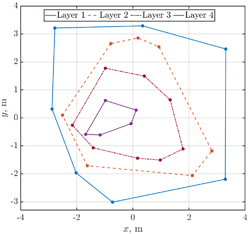
The convex layers [25] for a set of points are defined as the set of nested convex polygons formed using the following procedure: form the convex hull of the points in , delete the points from that form the vertices of the convex hull and continue the process until the number of points in is less than 3. Consider a set of randomly selected 26 points in a plane such that the and coordinates of points satisfy . For this example, Fig. 2 shows the formation of four convex layers using the aforementioned procedure. Some of the important properties of convex layers are:
-
(P1)
The set of convex layers for a set of points is unique.
-
(P2)
Each layer is a convex polygon.
-
(P3)
No two layers share a common vertex.
-
(P4)
For any two convex layers, one of the layers completely encompasses the other.
The procedure for forming convex layers is formally presented in Algorithm 1. Here denote the set of points where . The set of convex layers is denoted by where is the outermost layer and .
Input :
Output :
3 Circular Distribution Problem
Consider a planar region consisting of a swarm of point-sized agents. The kinematics of the th agent is governed by
| (3) |
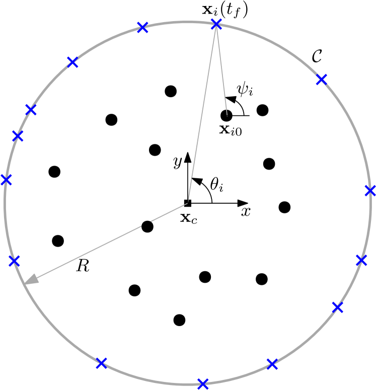
Here, and represent the position, the constant forward velocity, and the heading angle input, respectively, of the th agent. Let denote a circle where and are its center and radius, respectively, and the initial positions of the agents satisfy
| (4) |
where is the initial position of the th agent. The objective here is to determine such that at some finite time and in a collision-free manner, the th agent occupies a unique goal position on the circumference of , that is,
| (5) | ||||
| (6) |
Here, is the relative angular orientation of as measured in a fixed frame with its origin at . Fig. 3 shows a representative scenario of the problem. Further, this work considers the following assumptions:
-
(A1)
No two agents are initially collocated.
-
(A2)
Each agent is capable of moving in any direction.
-
(A3)
A centralized server has the initial position information of all agents.
-
(A4)
The server computes and communicates heading angle input for every agent.
-
(A5)
Low-level controllers track the prescribed and with negligible error.
4 Main Results
In this section, we propose a solution for determining a unique goal position on the circle for each agent and a conflict-free strategy for guiding the agents towards their respective goal position.
4.1 Proposed Goal Assignment Policy
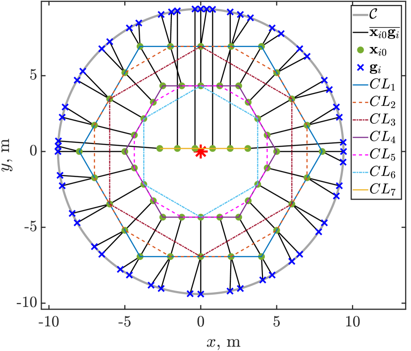
Using Algorithm 1, the set of convex layers is formed using the initial positions of the agents such that the set () stores the vertices of . Accordingly, each vertex of represents the initial position of an agent. Using Definition 3, the search space is constructed for the th agent. Let denotes the set of all points on . The set of potential goal positions, for the th agent is obtained from the intersection of and , that is,
| (7) |
In Fig. 4, the gray-shaded region and the green arc
¿
represent and of the th agent, respectively. The following theorem presents a strategy to determine the th agent’s goal position which offers the minimum Euclidean distance from .
Theorem 1
Consider the th agent with its position as expressed in polar coordinate system centered at (Fig. 4). Let intersect to obtain the arc ¿ such that the polar coordinates of and relative to are and , respectively . The goal position of the th agent for which it travels the minimum Euclidean distance to is
| (8) |
where .
Proof 4.2.
The distance between the th agent and a point can be expressed as:
| (9) |
Now, consider the problem
| (10) |
The Lagrangian Multiplier method is used to solve the constrained optimization problem in (10). The Lagrangian of the problem in (10) is expressed as
| (11) |
where are Lagrange multipliers. Let . Further, different combinations of active constraints are analyzed for and the feasibility of solutions is checked.
Case 1: . In this case, the Lagrangian in (11) reduces to , and the gradient and the Hessian of are
| (12) | ||||
| (13) |
In accordance with the first-order necessary condition, is evaluated using Eq. (12) to obtain the critical points of .
| (14) |
To determine the local minimum point from the critical points obtained in (14), the second-order necessary condition is checked by evaluating in (13) at , that is,
| (15) | ||||
| (16) |
Since from Eq. (15), the solution that minimizes is . Given , the solution is feasible when
| (17) | ||||
| Here, | (18) |
Case 2: . Here, using Eq. (11), the Lagrangian is obtained as , and the gradient and the Hessian of are
| (19) | ||||
| (20) |
Using Eq. (19) and applying the first-order necessary condition on to find its critical points,
| (21) | ||||
| (22) |
To check the second-order necessary condition, in (20) is evaluated at the point .
| (23) |
Let . Then, the eigenvalues of are
| (24) |
In (24), , the eigenvalues are mixed is indefinite and is a saddle point.
Case 3: . In this case, the Lagrangian in (11) is given by , and the gradient and the Hessian of are
| (25) | ||||
| (26) |
Following the first-order necessary condition, using Eq. (25),
| (27) | ||||
| (28) |
For the second-order necessary condition, is evaluated at as
| (29) |
Let . Accordingly, the eigenvalues of are
| (30) |
In (30), , the eigenvalues are mixed is indefinite and is a saddle point.
Two saddle points, and , are obtained from Cases 2 and 3, respectively. From Eq. (28), and from Eq. (22), . Combining both these cases, the two saddle points are now analyzed to find when .
| (31) |
Comparing and from Eq. (31),
| (32) | ||||
| (33) |
Case 4: . This case is infeasible as and both inequality constraints in (10) cannot be satisfied simultaneously.
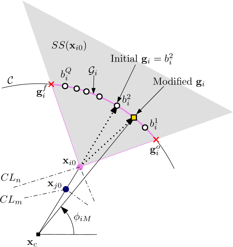
Following the goal assignment strategy discussed in Theorem 1, the next challenge is to ensure that each agent is assigned a unique goal. Although the policy proposed in (8) designates the goal position for each agent on the circumference of , it does not ensure a unique goal assignment for certain initial positional arrangements of the agents. An example of such a configuration is shown in Fig. 5 where and . Here, the goal positions for the th and the th agents are found to be collocated using the policy in (8).
To rule out the possibility of conflicting goal assignment, Algorithm 2 is proposed which assigns a unique goal for each of the agents irrespective of their initial positional arrangement. Algorithm 2 assigns goal positions in sequence, starting from the agents in , followed by , , and continuing until . Therein, is the set of goal positions assigned in previous iterations, and is the set of points in that lie on ¿ , that is,
| (34) |
Points in are assumed to be numbered clockwise around . A conflict for the th agent arises if
| (35) |
Consider the set where each element is defined by the angular position of the elements in the set with
| (36) |
For the case in (35), is recomputed as follows:
| (37) |
where is a constant. From Eq. (37), the direction of the shift in is clockwise/anti-clockwise if the angular separation of from its immediate neighboring point in is greater in the clockwise/anti-clockwise direction. The direction of the shift is conventionally chosen clockwise when . This procedure is formally presented in Algorithm 2. Consider again the example shown in Fig. 5. Using Algorithm 2, is modified as shown in Fig. 6.
Proposition 4.3.
The recomputed goal position of the th agent in (37) also lies in its set of potential goal positions, that is, .
Proof 4.4.
Remark 4.5.
Remark 4.6.
The heading angle input for the th agent is obtained by taking the argument of the vector , that is,
| (39) |
where and . Further, the final time is calculated by considering a straight line joining and with agent moving at constant speed , that is,
| (40) |
Remark 4.7.
The th agent employs a constant speed along obtained using (39) during the interval and stops when it reaches .
4.2 Result on Guaranteed Inter-agent Collision Avoidance
For the goal position assigned to each agent using Algorithm 2, Theorems (4.8) and (4.10) establish that there are no inter-agent collisions as the agents move towards their respective .
Theorem 4.8.
For the th agent in , a point satisfies the following relation:
| (41) |
where Conv.
Proof 4.9.
In Fig. 7, let be the included angle between the sides and of the triangle formed by the points . As shown in Fig. 7, let be the angles formed by the segment with the boundaries of , and be the angles formed by the segment with the supporting edges of . From the geometry in Fig. 7,
| (42) | ||||
| (43) |
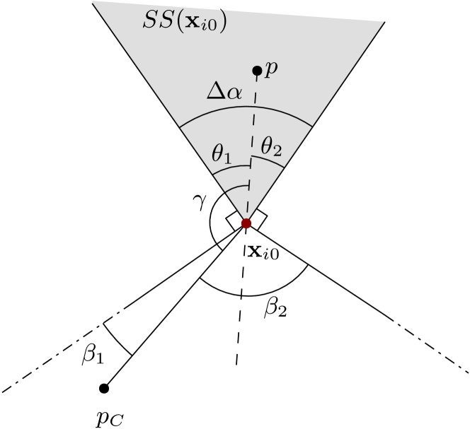
Here, is obtained as
| (44) |
Theorem 4.10.
Consider any two distinct agents and whose goal positions are and , respectively. As both agents move with the identical prescribed speed on the straight-line path connecting their initial positions to their respective goal positions, they do not collide.
Proof 4.11.
Consider . Without loss of generality, assume . From Algorithm 1, . Using Theorem 4.8,
| (45) |
From (45), reaches prior to as both agents move with the same speed . Hence , there is no collision between and .
For . Using the convex property of , the only point that lies on is . Since and , does not lie on the straight path joining and , that is, . This rules out any collision possibility for when .
5 Illustrative Examples
In this section, the proposed goal assignment policy in Algorithm 2 is demonstrated using MATLAB simulations through two examples, followed by a statistical analysis of the path length obtained for all agents. The prescribed speed of the agents m/s. The parameter in (37) is .
5.1 Example 1
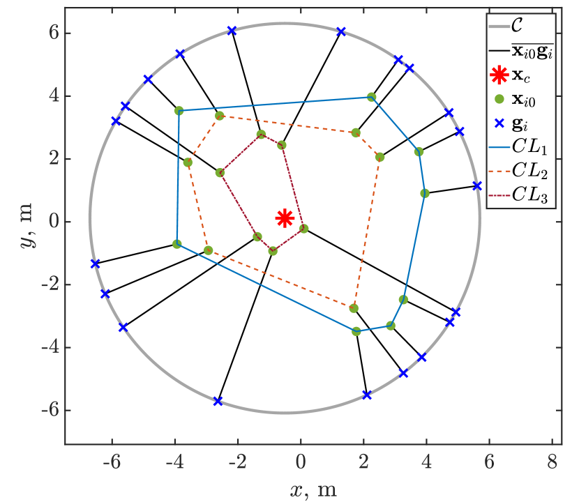
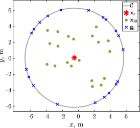
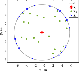
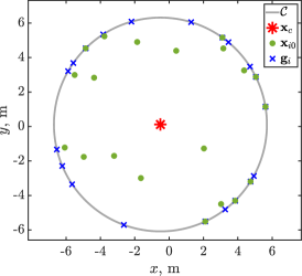
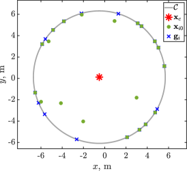
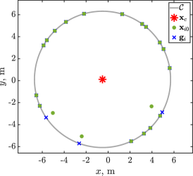
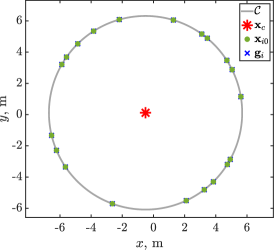
This example scenario considers 20 agents with initial positions chosen randomly within a rectangular region satisfying . The center of is (0.15, 0.06) and its radius is 5.03 m. The set of convex layers and the unique goal position for each agent are shown in Fig. 8. The time at which all agents reach , that is, s. Fig. 9 shows six consecutive snapshots of the simulation where the agents governed by (3) move to occupy their respective goal positions on .
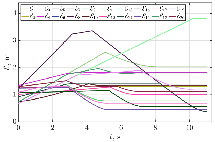
Further, is defined as the distance between the th agent and its closest neighbor, that is,
| (46) |
where . The time evolution of for all agents is shown in Fig. 10. Here, implies that the agents do not collide with each other.
5.2 Example 2
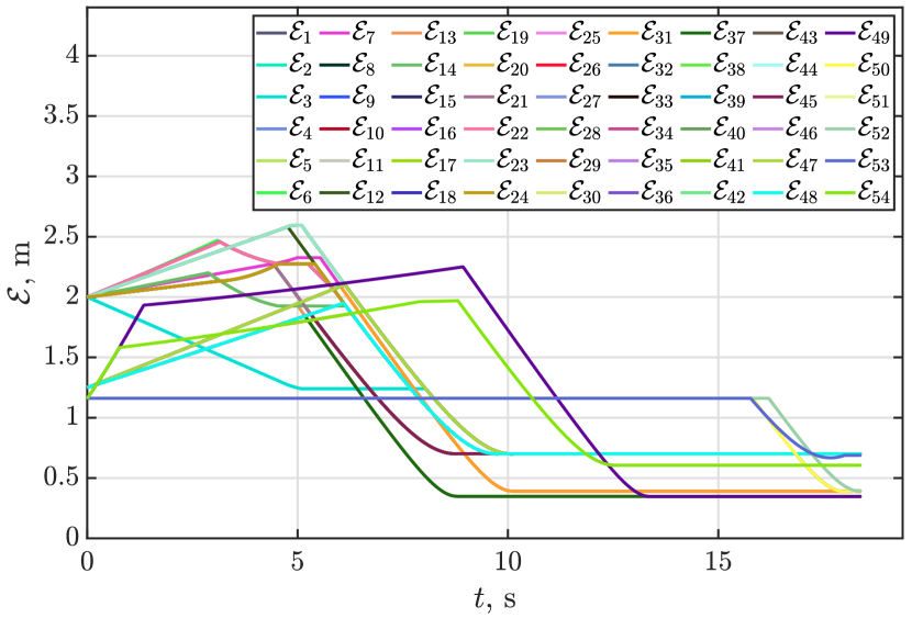
In this example, an initial arrangement of 54 agents distributed on two nested regular hexagons, with side lengths 8 and 6 m, and a line segment joining [-2.9,0] and [2.9,0] is considered. Therein, 24 agents are equispaced along the perimeter of each hexagon, and the remaining 6 agents are equispaced on the line segment. The center and radius of are [0,0] and m, respectively. A set of seven convex layers, that is, is formed using the initial positions of the agents. Fig. 11 shows the path followed by each agent to its respective goal position. The time taken for all agents to reach is 18.4 s. The variation of with time for all agents in Fig. 12 shows no inter-agent collision.
5.3 Monte Carlo Simulations
To quantitatively investigate the efficiency of the proposed goal assignment policy, Monte Carlo method is used. Therein, the initial positions of 20 agents are randomly sampled within the region considered in Example 1 for 100 scenarios.
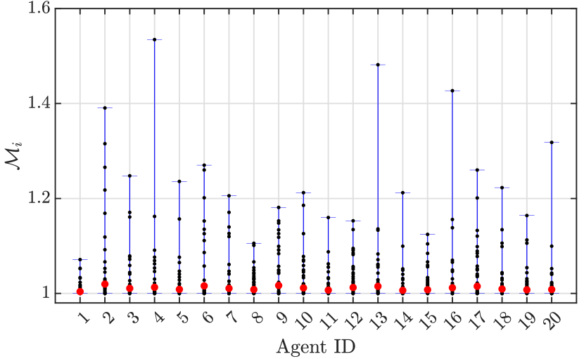
A performance metric is defined as the ratio of the distance covered by the th agent to the shortest distance required by that agent to reach , that is,
| (47) |
From (47), is aligned along the radial line . A higher value in indicates a greater deviation from the shortest possible path to . In Fig. 13, the values of in the 100 simulations are represented by black dots, while the red dot indicates the mean value of . The results are summarized in Table 1 where , for a scenario, measures the percentage increase in the sum of the path length for all agents compared to the sum of the shortest possible path length for all agents. Out of 100 scenarios, is found to be less than 5% in 97 of them.
| Number of scenarios | |
|---|---|
| 45 | |
| 31 | |
| 10 | |
| 7 | |
| 4 | |
| 3 |
6 Conclusion
This work presents a one-shot goal assignment policy for distributing multiple agents along a circular boundary encompassing the agents. Utilizing the geometry of convex layers, a search space region is proposed for each of the agents. Regardless of the initial arrangement of agents, the proposed goal assignment policy ensures a unique goal position for each agent within its search space region. A guarantee for inter-agent collision avoidance is established using the property that a point in the search space of an agent is closer to that agent as compared to any other agent lying within or on the convex layer on which the agent lies. A statistical analysis of path lengths in an example scenario shows that the average path length of agents remains very close to the average of the minimum Euclidean distance between their initial positions and the circular boundary. In contrast to the existing works, the proposed policy resolves conflicts at the initial time, and no further computations are required for detecting collisions, or altering speed or heading angle of the agents thereafter.
Future research directions include three-dimensional distribution of agents on regular or irregular boundaries.
References
- [1] J. Scherer and B. Rinner, “Multi-uav surveillance with minimum information idleness and latency constraints,” IEEE Robotics and Automation Letters, vol. 5, no. 3, pp. 4812–4819, 2020.
- [2] Y. Tian, K. Liu, K. Ok, L. Tran, D. Allen, N. Roy, and J. P. How, “Search and rescue under the forest canopy using multiple uavs,” 2020.
- [3] D. K. D. Villa, A. S. Brandão, and M. Sarcinelli-Filho, “Path-following and attitude control of a payload using multiple quadrotors,” in 2019 19th International Conference on Advanced Robotics (ICAR), pp. 535–540, 2019.
- [4] S. Ivić, A. Andrejčuk, and S. Družeta, “Autonomous control for multi-agent non-uniform spraying,” Applied Soft Computing, vol. 80, pp. 742–760, 2019.
- [5] J. Ma, W. Yao, W. Dai, H. Lu, J. Xiao, and Z. Zheng, “Cooperative encirclement control for a group of targets by decentralized robots with collision avoidance,” in 2018 37th Chinese Control Conference (CCC), pp. 6848–6853, IEEE, 2018.
- [6] N. E. Leonard, D. A. Paley, F. Lekien, R. Sepulchre, D. M. Fratantoni, and R. E. Davis, “Collective motion, sensor networks, and ocean sampling,” Proceedings of the IEEE, vol. 95, no. 1, pp. 48–74, 2007.
- [7] C. Song, L. Liu, and S. Xu, “Circle formation control of mobile agents with limited interaction range,” IEEE Transactions on Automatic Control, vol. 64, no. 5, pp. 2115–2121, 2018.
- [8] I. Suzuki and M. Yamashita, “Distributed anonymous mobile robots: Formation of geometric patterns,” SIAM J. Comput., vol. 28, pp. 1347–1363, 1999.
- [9] P. Flocchini, G. Prencipe, N. Santoro, and G. Viglietta, “Distributed computing by mobile robots: Uniform circle formation,” 2017.
- [10] R. Yang, A. Azadmanesh, and H. Farhat, “Polygon formation in distributed multi-agent systems.,” International Journal for Computers & Their Applications, vol. 30, no. 2, 2023.
- [11] R. Vaidyanathan, G. Sharma, and J. Trahan, “On fast pattern formation by autonomous robots,” Information and Computation, p. 104699, 2021.
- [12] S. Huang, W. Cui, J. Cao, and R. S. H. Teo, “Self-organizing formation control of multiple unmanned aerial vehicles,” in IECON 2019 - 45th Annual Conference of the IEEE Industrial Electronics Society, vol. 1, pp. 5287–5291, 2019.
- [13] S. Jiang, J. Cao, J. Wang, M. Stojmenovic, and J. Bourgeois, “Uniform circle formation by asynchronous robots: A fully-distributed approach,” in 2017 26th International Conference on Computer Communication and Networks (ICCCN), pp. 1–9, 2017.
- [14] J. Alonso-Mora, A. Breitenmoser, M. Rufli, R. Siegwart, and P. Beardsley, “Multi-robot system for artistic pattern formation,” in 2011 IEEE International Conference on Robotics and Automation, pp. 4512–4517, IEEE, 2011.
- [15] B. Katreniak, “Biangular circle formation by asynchronous mobile robots,” in International Colloquium on Structural Information and Communication Complexity, pp. 185–199, Springer, 2005.
- [16] G. A. Di Luna, R. Uehara, G. Viglietta, and Y. Yamauchi, “Gathering on a circle with limited visibility by anonymous oblivious robots,” arXiv preprint arXiv:2005.07917, 2020.
- [17] C. Feletti, C. Mereghetti, and B. Palano, “Uniform circle formation for swarms of opaque robots with lights,” in Stabilization, Safety, and Security of Distributed Systems: 20th International Symposium, SSS 2018, Tokyo, Japan, November 4–7, 2018, Proceedings 20, pp. 317–332, Springer, 2018.
- [18] S. Das, P. Flocchini, G. Prencipe, and N. Santoro, “Forming sequences of patterns with luminous robots,” IEEE Access, vol. 8, pp. 90577–90597, 2020.
- [19] R. Adhikary, M. K. Kundu, and B. Sau, “Circle formation by asynchronous opaque robots on infinite grid,” Computer Science, vol. 22, Feb. 2021.
- [20] X. Défago and A. Konagaya, “Circle formation for oblivious anonymous mobile robots with no common sense of orientation,” (New York, NY, USA), Association for Computing Machinery, 2002.
- [21] R. L. Graham, “An efficient algorithm for determining the convex hull of a finite planar set,” Info. Pro. Lett., vol. 1, pp. 132–133, 1972.
- [22] D. R. Smith, “The design of divide and conquer algorithms,” Science of Computer Programming, vol. 5, pp. 37–58, 1985.
- [23] T. M. Chan, “Optimal output-sensitive convex hull algorithms in two and three dimensions,” Discrete Comput. Geom., vol. 16, p. 361–368, apr 1996.
- [24] M. G. Resende and P. M. Pardalos, Handbook of optimization in telecommunications. Springer Science & Business Media, 2008.
- [25] B. Chazelle, “On the convex layers of a planar set,” IEEE Transactions on Information Theory, vol. 31, no. 4, pp. 509–517, 1985.