When time delays and phase lags are not the same: higher-order phase reduction unravels delay-induced synchronization in oscillator networks

Christian Bick1,2,3,4, Bob Rink1, and Babette A. J. de Wolff1 1Department of Mathematics, Vrije Universiteit Amsterdam, Amsterdam, the Netherlands
2Mathematical Insititute, University of Oxford, Oxford, UK
3Department of Mathematics, University of Exeter, Exeter, UK
4Institute for Advanced Study, Technische Universität München, Garching, Germany
Abstract

Coupled oscillators with time-delayed network interactions are critical to understand synchronization phenomena in many physical systems. Phase reductions to finite-dimensional phase oscillator networks allow for their explicit analysis. However, first-order phase reductions—where delays correspond to phase lags—fail to capture the delay-dependence of synchronization. We develop a systematic approach to derive phase reductions for delay-coupled oscillators to arbitrary order. Already the second-order reduction can predict delay-dependent (bi-)stability of synchronized states as demonstrated for Stuart–Landau oscillators.

Time delays in network interactions—induced by finite transmission speed for instance—shape the synchronization behavior of coupled oscillator networks [1]. It is crucial to determine how time delay affects synchronization, not only to understand complex physical systems, such as brain dynamics and function [2, 3], but also to control them [4, 5]. Phase reduction, i.e., deriving the dynamics of the phases ϕj𝕋:=/2πsubscriptitalic-ϕ𝑗𝕋assign2𝜋\phi_{j}\in\mathbb{T}:=\mathbb{R}/2\pi\mathbb{Z} of the oscillators, is a widely used dimension-reduction technique to analyze synchronization behaviour of coupled oscillator networks [6, 7, 8]. Since the seminal work by Kuramoto and Sakaguchi [9, 10], the standard approach to account for time delays is to approximate them by phase lags: If oscillator j𝑗j evolves at frequency ωjsubscript𝜔𝑗\omega_{j} in isolation, then its phase at time time tτ𝑡𝜏t-\tau is approximated by ϕj(tτ)ϕj(t)ωjτsubscriptitalic-ϕ𝑗𝑡𝜏subscriptitalic-ϕ𝑗𝑡subscript𝜔𝑗𝜏\phi_{j}(t-\tau)\approx\phi_{j}(t)-\omega_{j}\tau. For coupling strength ε𝜀\varepsilon, this approximation is generally valid only if ετ𝜀𝜏\varepsilon\tau is small [11]. This, however, significantly limits the applicability of the phase-lag approximation for many physically relevant systems: 
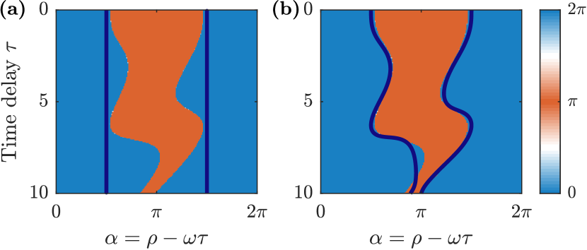
It fails to capture basic network synchronization properties even for moderate coupling strength and/or delays; cf. Fig. 1(a).

In this paper, we develop a systematic approach to phase reduction for delay-coupled oscillators, thereby clarifying how time delays affect the phase dynamics. Mathematical theory [12, 13] shows that $n$ delay-coupled oscillators—an infinite-dimensional system—generally give rise to finite-dimensional phase dynamics on $\mathbb{T}^{n}$ (rather than phase equations with time delay [14]). Computing these phase dynamics, however, has remained elusive. Our approach first reformulates the delay differential equation as an ordinary differential equation coupled to a transport equation. Then, we use a parametrization method [15] to compute the phase reduction order-by-order. This approach naturally recovers the phase-lag approximation at first order: The first-order phase dynamics is determined by the uncoupled zeroth-order evolution $\phi_{j}(t)=\phi_{j}(0)+\omega_{j}t$ for which a time delay is a phase lag. By contrast, the second-order approximation is determined by the nontrivial solutions of the first-order dynamics. Hence, the phase dynamics of order two and higher will depend non-trivially on the delay, in a way that we can compute explicitly.

Refer to caption
Figure 1: Time-delayed coupling influences the synchronization of two coupled Stuart–Landau oscillators (9) with states $z_{j}=r_{j}\mathrm{e}^{\phi_{j}}$ for parameters $a=b=1$ and coupling strength $\varepsilon=0.1$. The coloring shows the phase difference $\psi=\phi_{1}-\phi_{2}$ after $T=1000$ time units from an initial condition $(z_{1}(0),z_{2}(0))=(\mathrm{e}^{0i},\mathrm{e}^{0.01i})$ close to in-phase synchrony $\{z_{1}=z_{2}\}$: Blue indicates convergence to in-phase synchrony and red convergence to anti-phase synchrony $\{z_{1}=iz_{2}\}$. The stability boundaries of in-phase synchrony predicted by phase reduction are shown by blue curves: The first-order approximation (12) gives the vertical lines in Panel (a) as time delays correspond to phase lags. By contrast, the second-order approximation (13) captures the delay-dependence of synchronization beyond small $\tau$, as shown in Panel (b).

Our approach provides a new way to understand delay-induced synchronization phenomena: Computing the second-order phase reduction explicitly for two coupled Stuart–Landau (SL) oscillators demonstrates the nontrivial dependence of the synchronization dynamics on the time delay. As shown in Fig. 1(b), already the second-order approximation of the two-dimensional phase dynamics correctly predicts synchronization in the original infinite-dimensional delay-coupled equations.

Methodology: Delay through transport.—We consider a general model of $n$ nonlinear oscillators coupled with transmission delay. In isolation, the state $x_{j}\in\mathbb{R}^{m_{j}}$ of oscillator $j$ evolves according to $\dot{x}_{j}(t)=F_{j}(x_{j}(t))$ which admits a $T_{j}$-periodic limit cycle $x_{j}^{*}(t)$ of frequency $\omega_{j}=\frac{2\pi}{T_{j}}$. In other words, the (asymptotic) state of each oscillator is determined by the phase $\phi_{j}\in\mathbb{T}$ of the point $x_{j}^{*}(\phi_{j}/\omega_{j})$ on the $j$th limit cycle. For coupling strength $\varepsilon>0$, oscillator $j\in\{1,\dotsc,n\}$ evolves according to

$\displaystyle\dot{x}_{j}(t)=F_{j}(x_{j}(t))+\varepsilon\sum_{k=1}^{n}G_{j,k}\left(x_{j}(t),x_{k}(t-\tau_{j,k})\right),$ (1)

where the function $G_{j,k}$ specifies the coupling from oscillator $k$ to $j$ and $\tau_{j,k}\geq 0$ the time delay. We seek to compute the ordinary differential equations that determine the the evolution of $\boldsymbol{\phi}=(\phi_{1},\dotsc,\phi_{n})^{\mathsf{T}}\in\mathbb{T}^{n}$ as an expansion in the coupling strength $\varepsilon\geq 0$:

$\displaystyle\dot{\boldsymbol{\phi}}={\mbox{\boldmath$f$}{}}({\boldsymbol{\phi}},\varepsilon)=\mbox{\boldmath$\omega$}{}+\varepsilon{\mbox{\boldmath$f$}{}}^{(1)}(\boldsymbol{\phi})+\varepsilon^{2}{\mbox{\boldmath$f$}{}}^{(2)}(\boldsymbol{\phi})+\dotsb.$ (2)

Here $\mbox{\boldmath$\omega$}{}=(\omega_{1},\dotsc,\omega_{n})^{\mathsf{T}}$ determines the uncoupled (zeroth-order) dynamics and ${\mbox{\boldmath$f$}{}}^{(\ell)}$ is its correction of order $\ell$.

The first step in our approach is to replace Eq. (1) by an ordinary differential equation coupled to a transport equation. Specifically, we consider the co-evolution of oscillator histories $X_{j}(s,t)$ and states $x_{j}(t)=X_{j}(0,t)$ given by

$\displaystyle\dot{x}_{j}(t)=F_{j}(x_{j}(t))+\varepsilon\sum_{k=1}^{n}G_{j,k}\left(x_{j}(t),X_{k}(-\tau_{j,k},t)\right)$ (3a)
$\displaystyle\partial_{t}X_{j}(s,t)=\partial_{s}X_{j}(s,t).$ (3b)

Note that problems (1) and (3) are equivalent: Solutions to the transport equation (3b) with boundary condition $X_{j}(0,t)=x_{j}(t)$ are given by $X_{j}(s,t)=x_{j}(t+s)$. In other words, $s\mapsto X_{j}(s,t)$ is the history of $x_{j}$ up to time $t$, parametrized by the history variable $s\in(-\infty,0]$.

In the second step, we match the phase dynamics (2) to be computed to the dynamics of the coupled system (3). To this end, we seek functions $e$, $E$ that relate solutions $\boldsymbol{\phi}(t)$ of the phase dynamics (2) to solutions $\mbox{\boldmath$X$}{}(s,t)=(X_{1}(s,t),\dotsc,X_{n}(s,t))^{\mathsf{T}}$, $\mbox{\boldmath$x$}{}(t)=(x_{1}(t),\dotsc,x_{n}(t))^{\mathsf{T}}$ of (3) through

$\displaystyle\mbox{\boldmath$x$}{}(t)$ $\displaystyle=\mbox{\boldmath$e$}{}(\boldsymbol{\phi}(t),\varepsilon),$ $\displaystyle\mbox{\boldmath$X$}{}(s,t)$ $\displaystyle=\mbox{\boldmath$E$}{}(s,\boldsymbol{\phi}(t),\varepsilon)$ (4)

with boundary condition $\mbox{\boldmath$e$}{}(\boldsymbol{\phi},\varepsilon)=\mbox{\boldmath$E$}{}(0,\boldsymbol{\phi},\varepsilon)$. Substitution of (2) and (4) into (3) gives

$\displaystyle\partial_{\boldsymbol{\phi}}e_{j}(\boldsymbol{\phi},\varepsilon)\cdot{\mbox{\boldmath$f$}{}}(\boldsymbol{\phi},\varepsilon)$ $\displaystyle={F}_{j}(e_{j}({\boldsymbol{\phi}},\varepsilon))$
$\displaystyle+\,\varepsilon\sum_{k}G_{j,k}(e_{j}(\boldsymbol{\phi},\varepsilon),E_{k}(-\tau_{j,k},\boldsymbol{\phi},\varepsilon)),$ (5a)
$\displaystyle\partial_{\boldsymbol{\phi}}E_{j}(s,\boldsymbol{\phi},\varepsilon)\cdot{\mbox{\boldmath$f$}{}}(\boldsymbol{\phi},\varepsilon)$ $\displaystyle=\partial_{s}E_{j}(s,\boldsymbol{\phi},\varepsilon).$ (5b)

Fulfilling these conjugacy equations links ${\mbox{\boldmath$e$}{}}(\boldsymbol{\phi})$, ${\mbox{\boldmath$E$}{}}(\boldsymbol{\phi})$ and the phase dynamics ${\mbox{\boldmath$f$}{}}(\boldsymbol{\phi})$ to the dynamics of (3)—and thus (1).

The third step is to expand (5) in powers of $\varepsilon$ to obtain iterative equations to determine ${\mbox{\boldmath$e$}{}}(\boldsymbol{\phi})$, ${\mbox{\boldmath$E$}{}}(\boldsymbol{\phi})$, and ${\mbox{\boldmath$f$}{}}(\boldsymbol{\phi})$. Write

$\displaystyle\mbox{\boldmath$e$}{}(\boldsymbol{\phi}(t),\varepsilon)$ $\displaystyle=\mbox{\boldmath$e$}{}^{(0)}(\boldsymbol{\phi}(t))+\varepsilon\mbox{\boldmath$e$}{}^{(1)}(\boldsymbol{\phi}(t))+\dotsb$
$\displaystyle\mbox{\boldmath$E$}{}(s,\boldsymbol{\phi}(t),\varepsilon)$ $\displaystyle=\mbox{\boldmath$E$}{}^{(0)}(s,\boldsymbol{\phi}(t))+\varepsilon\mbox{\boldmath$E$}{}^{(1)}(s,\boldsymbol{\phi}(t))+\dotsb$

and substitute this, together with (2), into (5). Collecting zero-th-order ($\varepsilon^{0}$) terms in (5) gives

$\displaystyle\partial_{\boldsymbol{\phi}}e_{j}^{(0)}(\boldsymbol{\phi})\cdot\mbox{\boldmath$\omega$}{}$ $\displaystyle={F_{j}}(e^{(0)}_{j}(\boldsymbol{\phi}))$ (6a)
$\displaystyle\partial_{\boldsymbol{\phi}}E_{j}^{(0)}(s,\boldsymbol{\phi})\cdot\mbox{\boldmath$\omega$}{}$ $\displaystyle=\partial_{s}E_{j}^{(0)}(s,\boldsymbol{\phi}).$ (6b)

For $\ell\geq 1$, collecting $\ell$th-order ($\varepsilon^{\ell}$) terms in (5) yields

$\displaystyle\partial_{\boldsymbol{\phi}}e^{(0)}_{j}(\boldsymbol{\phi})\cdot\mbox{\boldmath$f$}{}^{(\ell)}(\boldsymbol{\phi})+\partial_{\boldsymbol{\phi}}e^{(\ell)}_{j}(\boldsymbol{\phi})\cdot\mbox{\boldmath$\omega$}{}\hskip 7.11317pt$
$\displaystyle-DF_{j}(e^{(0)}_{j}(\boldsymbol{\phi}))\cdot{e_{j}}^{(\ell)}(\boldsymbol{\phi})$ $\displaystyle=h_{j}^{(\ell)}(\boldsymbol{\phi})$ (7a)
$\displaystyle\partial_{\boldsymbol{\phi}}E_{j}^{(\ell)}(s,\boldsymbol{\phi})\cdot{\mbox{\boldmath$\omega$}{}}-\partial_{s}E_{j}^{(\ell)}(s,\boldsymbol{\phi})$ $\displaystyle=H_{j}^{(\ell)}(s,\boldsymbol{\phi})$ (7b)

where $DF_{j}$ denotes the $(m_{j}\times m_{j})$-Jacobian matrix of $F_{j}$, while $h_{j}^{(\ell)}$ and $H_{j}^{(\ell)}$ are inhomogeneous terms that can be computed explicitly from the lower-order expressions. For instance, for $\ell=1$ these terms are given by

$\displaystyle h_{j}^{(1)}(\boldsymbol{\phi})=\sum_{k}G_{j,k}\big{(}e_{j}^{(0)}(\boldsymbol{\phi}),E_{k}^{(0)}(-\tau_{j,k},\boldsymbol{\phi})\big{)},$
$\displaystyle H_{j}^{(1)}(s,\boldsymbol{\phi})=-\partial_{\boldsymbol{\phi}}E_{j}^{(0)}(s,\boldsymbol{\phi})\cdot\mbox{\boldmath$f$}{}^{(1)}(\boldsymbol{\phi}).$

Thus, (7) forms a system of inductive equations that determine the phase dynamics to arbitrary order $\ell$.

The fourth step is now to solve these equations order-by-order. The zeroth-order equations (6) have solution $e_{j}^{(0)}(\boldsymbol{\phi})=x_{j}^{*}(\phi_{j}/\omega_{j})$, $E_{j}^{(0)}(s,\boldsymbol{\phi})=e_{j}^{(0)}(\boldsymbol{\phi}+\mbox{\boldmath$\omega$}{}s)=x_{j}^{*}(\phi_{j}/\omega_{j}+s)$, i.e., the periodic orbits of the uncoupled system. At first-order ($\ell=1$), equation (7a) is a system of inhomogeneous linear equations for $\mbox{\boldmath$e$}{}^{(1)}$ and $\mbox{\boldmath$f$}{}^{(1)}$ that depend on $\mbox{\boldmath$e$}{}^{(0)}$, $\mbox{\boldmath$E$}{}^{(0)}$. These equations can be solved in exactly the same way as for problems without time delay, for example using Floquet theory [15]. Because the inhomogeneous terms $h_{j}^{(1)}(\boldsymbol{\phi})$ depend on $E_{k}^{(0)}(-\tau_{j,k},\boldsymbol{\phi})=e_{k}^{(0)}(\boldsymbol{\phi}-\mbox{\boldmath$\omega$}{}\tau_{j,k})$, the delays $\tau_{j,k}$ appear in $\mbox{\boldmath$e$}{}^{(1)}$ and $\mbox{\boldmath$f$}{}^{(1)}$ through phase lags of the unperturbed periodic orbits, as expected. The first-order equation (7b) is an inhomogeneous linear transport equation for $\mbox{\boldmath$E$}{}^{(1)}$. It can be solved using the method of characteristics, which—with boundary condition $\mbox{\boldmath$E$}{}^{(1)}(0,\boldsymbol{\phi})=\mbox{\boldmath$e$}{}^{(1)}(\boldsymbol{\phi})$—gives

$$\begin{split}E_{j}^{(1)}(s,\boldsymbol{\phi})&=e_{j}^{(1)}(\boldsymbol{\phi}+\mbox{\boldmath$\omega$}{}s)\\ &\qquad\quad-\int_{0}^{s}H_{j}^{(1)}\big{(}\sigma,\boldsymbol{\phi}+\mbox{\boldmath$\omega$}{}(s-\sigma)\big{)}\,\mathrm{d}\sigma.\end{split}$$ (8)

Equations (7) for order $\ell>1$ have the same structure: They consist of a system of inhomogeneous linear equations for $\mbox{\boldmath$e$}{}^{(\ell)}$ and $\mbox{\boldmath$f$}{}^{(\ell)}$ that can be solved with Floquet theory, and a system of inhomogeneous transport equations for $\mbox{\boldmath$E$}{}^{(\ell)}$ that can be solved by the method of characteristics. Our method thus allows to analytically compute phase reductions of (1) to arbitrary order in the coupling strength $\varepsilon$.

Delay-coupled Stuart–Landau oscillators.—As a proof of principle, we apply our method to compute second-order phase equations for two identical delay-coupled Stuart–Landau (SL) oscillators

$\displaystyle\dot{z}_{1}$ $\displaystyle=(a+ib)z_{1}-\left|z_{1}\right|^{2}z_{1}+\varepsilon\mathrm{e}^{i\rho}\left(z_{2}(t-\tau)-z_{1}\right)$ (9)
$\displaystyle\dot{z}_{2}$ $\displaystyle=(a+ib)z_{2}-\left|z_{2}\right|^{2}z_{2}+\varepsilon\mathrm{e}^{i\rho}\left(z_{1}(t-\tau)-z_{2}\right)$

with $z_{j}\in\mathbb{C}$ and $i:=\sqrt{-1}$. We assume that $a>0$ and $b\neq 0$, so that in the absence of coupling, the SL oscillators possess identical limit cycles $z_{j}^{*}(t)=\sqrt{a}\mathrm{e}^{ibt}$ of frequency $\omega:=\omega_{j}=b$. As a result we have $e_{j}^{(0)}(\boldsymbol{\phi})=\sqrt{a}\mathrm{e}^{i\phi_{j}}$, $E_{j}^{(0)}(s,\boldsymbol{\phi})=\sqrt{a}\mathrm{e}^{i(\phi_{j}+\omega s)}$ and $\mbox{\boldmath$\omega$}{}=(\omega,\omega)^{\mathsf{T}}$ to order $\varepsilon^{0}$.

The symmetry of the problem allows to avoid the use of Floquet theory to solve the first-order equations and instead make the phase-difference ansatz

$\displaystyle\mbox{\boldmath$e$}{}^{(1)}(\boldsymbol{\phi})$ $\displaystyle=(e^{i\phi_{1}}A(\phi_{2}-\phi_{1}),e^{i\phi_{2}}A(\phi_{1}-\phi_{2}))^{\mathsf{T}},$
$\displaystyle\mbox{\boldmath$f$}{}^{(1)}(\boldsymbol{\phi})$ $\displaystyle=(B(\phi_{2}-\phi_{1}),B(\phi_{1}-\phi_{2}))^{\mathsf{T}},$

with real-valued functions $A,B$ on $\mathbb{T}$. This transforms (7) into the single complex equation

$\displaystyle i\sqrt{a}B(\theta)+2aA(\theta)$ $\displaystyle=\sqrt{a}\mathrm{e}^{i\rho}(\mathrm{e}^{i(\theta-\omega\tau)}-1).$ (10)

Equation (10) is readily solved for $A(\theta)$ and $B(\theta)$ by examining its real and imaginary parts separately, yielding

$\displaystyle\mbox{\boldmath$f$}{}^{(1)}(\boldsymbol{\phi})$ $\displaystyle=\begin{pmatrix}\sin(\phi_{2}-\phi_{1}-\omega\tau+\rho)-\sin(\rho)\\ \sin(\phi_{1}-\phi_{2}-\omega\tau+\rho)-\sin(\rho)\end{pmatrix}$ (11)
and
$\displaystyle\mbox{\boldmath$e$}{}^{(1)}(\boldsymbol{\phi})$ $\displaystyle=\frac{1}{2\sqrt{a}}\!\begin{pmatrix}\mathrm{e}^{i\phi_{1}}\left[\cos(\phi_{2}-\phi_{1}-\omega\tau+\rho)-\cos(\rho)\right]\\ \mathrm{e}^{i\phi_{2}}\left[\cos(\phi_{1}-\phi_{2}-\omega\tau+\rho)-\cos(\rho)\right]\end{pmatrix},$

which describe the first-order phase dynamics. Note the phase lag in (11). We calculate $\mbox{\boldmath$E$}{}^{(1)}$ from (8) to obtain

$\displaystyle\mbox{\boldmath$E$}{}^{(1)}(s,\boldsymbol{\phi})=\mbox{\boldmath$e$}{}^{(1)}(\phi_{1}+\omega s,\phi_{2}+\omega s)$
$\displaystyle+s\begin{pmatrix}i\sqrt{a}\mathrm{e}^{i(\phi_{1}+\omega s)}\left[\sin(\phi_{2}-\phi_{1}-\omega\tau+\rho)-\sin(\rho)\right]\\ i\sqrt{a}\mathrm{e}^{i(\phi_{2}+\omega s)}\left[\sin(\phi_{1}-\phi_{2}-\omega\tau+\rho)-\sin(\rho)\right]\end{pmatrix}.$

The second term in the formula shows the nontrivial dependence on the history variable $s$.

For the second-order approximation, note that $\mbox{\boldmath$E$}{}^{(1)}(-\tau,\boldsymbol{\phi})$ enters into the inhomogeneity ${\mbox{\boldmath$h$}{}}^{(2)}$ of the iterative equations that determine ${\mbox{\boldmath$f$}{}}^{(2)}$ and ${\mbox{\boldmath$e$}{}}^{(2)}$. We can therefore expect $\mbox{\boldmath$f$}{}^{(2)}$ to depend on the time delay $\tau$ in a nontrivial fashion. Solving the corresponding second-order equations as explained above—details are given in [16]—we find

$\displaystyle\mbox{\boldmath$f$}{}^{(2)}(\boldsymbol{\phi})=\left[\frac{1}{4a}-\frac{\tau}{2}\right]\sin(2\rho-2\omega\tau)\begin{pmatrix}1\\ 1\end{pmatrix}$
$\displaystyle+\tau\sin(\rho)\begin{pmatrix}\cos(\phi_{2}-\phi_{1}-\omega\tau+\rho)\\ \cos(\phi_{1}-\phi_{2}-\omega\tau+\rho)\end{pmatrix}$
$\displaystyle+\frac{\tau}{2}\cos(2\rho-2\omega\tau)\begin{pmatrix}\sin(2(\phi_{2}-\phi_{1}-\omega\tau+\rho))\\ \sin(2(\phi_{1}-\phi_{2}-\omega\tau+\rho))\end{pmatrix}$
$\displaystyle-\left[\frac{1}{4a}+\frac{\tau}{2}\right]\sin(2\rho-2\omega\tau)\begin{pmatrix}\cos(2(\phi_{2}-\phi_{1}-\omega\tau+\rho))\\ \cos(2(\phi_{1}-\phi_{2}-\omega\tau+\rho))\end{pmatrix}.$

Together with (11), this specifies the phase dynamics (2) and its dependence on the delay up to second order; we omit explicit expressions of $\mbox{\boldmath$e$}{}^{(2)}$ and $\mbox{\boldmath$E$}{}^{(2)}$ as they are not relevant for the phase dynamics.

Phase reduction shows delay-dependent synchronization.—The phase equations that we derived for (9) elucidate how the synchronization of the network depends on the time delay $\tau$. Introducing the phase difference coordinate $\psi:=\phi_{1}-\phi_{2}$ yields effective one-dimensional dynamics. In-phase synchrony corresponds to the equilibrium $\psi=0$ and anti-phase synchrony to the equilibrium $\psi=\pi$. Thus, the stability of these equilibria is crucial to understand the synchronization dynamics of the delay-coupled oscillator network.

To first order, the time delay enters as a phase lag. Specifically, the phase equations (2) truncated at first order imply that the phase difference $\psi$ evolves according to

$$\dot{\psi}=-2\varepsilon\cos(\rho-\omega\tau)\sin(\psi).$$ (12)

governed by a single harmonic. The first-order approximation thus predicts that the synchronization behavior is fully determined by the effective phase lag $\alpha=\rho-\omega\tau$: The equilibrium $\psi=0$ is linearly stable for $\alpha\in(-\frac{\pi}{2},\frac{\pi}{2})$, the equilibrium $\psi=\pi$ is linearly stable for $\alpha\in(\frac{\pi}{2},\frac{3\pi}{2})$, and there is an exchange of stability in a degenerate bifurcation at $\alpha\in\{\frac{\pi}{2},\frac{3\pi}{2}\left(\equiv-\frac{\pi}{2}\right)\}$. These stability boundaries are depicted in Fig. 1(a) as vertical lines. At the same time, solving the time-delayed differential equations (9) numerically shows that for coupling strength $\varepsilon=0.1$ the first-order approximation breaks down for time delays well below one period of the uncoupled SL oscillators; cf. the shading in Fig. 1(a).

The second-order phase equations do capture the delay-dependence of the synchronization. With $\alpha=\rho-\omega\tau$ as above, the phase dynamics (2) truncated at second order evaluates to

$\displaystyle\dot{\psi}$ $\displaystyle=-2\left(\varepsilon\cos(\alpha)-\varepsilon^{2}\tau\sin(\rho)\sin(\alpha)\right)\sin(\psi)$ (13)
$\displaystyle\qquad-\varepsilon^{2}\left(\tau+\frac{1}{2a}\sin^{2}(2\alpha)\right)\sin(2\psi).$

Note that the second-order terms introduce a second harmonic, and make the Fourier coefficients depend explicitly on the time delay $\tau$. Linear stability of in-phase synchrony $\psi=0$ is determined by the Lyapunov exponent

$$\lambda^{(0)}=\cos(\alpha)+\varepsilon\left(\tau+\frac{1}{2\alpha}\sin^{2}(2\alpha)-\tau\sin(\rho)\sin(\alpha)\right).$$

The bifurcation curves $\lambda^{(0)}=0$ are colored blue in Fig. 1(b). They not only provide a more accurate approximation of the numerical simulations (coloring), but also qualitatively capture the delay-dependence of the synchronization transition.

Refer to caption
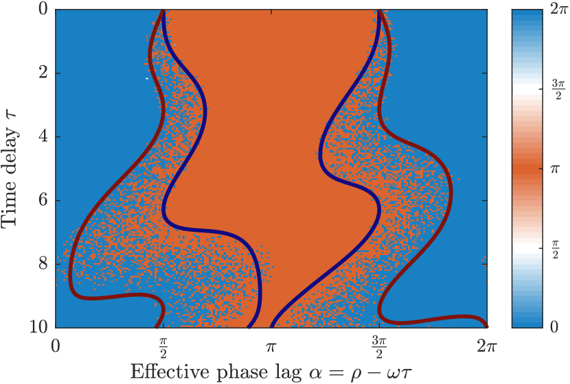
Figure 2: Random initial conditions show delay-dependent regions of bistability between in-phase synchrony and anti-phase synchrony for coupled SL oscillators (9); parameters and coloring are chosen as in Fig. 1. The curves indicate the stability boundaries predicted by the second-order phase reduction (13) for in-phase synchrony (dark blue, as in Fig. 1) determined by $\lambda^{(0)}=0$, and anti-phase synchrony (dark red) determined by $\lambda^{(\pi)}=0$.

The second-order phase equations also capture delay-dependent multistability. Indeed, simulations of the delay-coupled SL oscillators (9) with random initial conditions show that there is a large (delay-dependent) range of parameters for which the system exhibits bistability between in-phase and anti-phase synchrony; this corresponds to the speckled area in Fig. 2. Computing the Lyapunov exponent $\lambda^{(\pi)}$ of $\psi=\pi$ in addition to $\lambda^{(0)}$ yields approximate bounds for the domain of bistability, for a coupling strength of $\varepsilon=0.1$ and delays of the order of one period of oscillation (blue/red lines in Fig. 2).

Discussion.—Our approach explains why even simple oscillators can show complex delay-dependent synchronization behavior that is not captured by a phase-lag approximation. In the example of coupled Stuart–Landau oscillators, the first-order phase equation (12) is given by a single harmonic function. First-order phase reduction is thus of limited use in predicting phase synchronisation, as a single harmonic cannot predict bistability of in-phase and anti-phase synchrony. For more complicated oscillators—such as oscillations close to a relaxation limit—one expects that already the first-order phase dynamics displays multiple harmonics [17]. While this implies that multistability can already be detected at first order, the correct delay-dependence will generally only be apparent to second order.

Applying our phase reduction method to larger networks is straightforward and will shed light on how time delays affect phase interactions to arbitrary order. Even if the coupling between nonlinear oscillators is additive—as in (1)—phase interactions beyond first order will display nonpairwise terms that describe indirect phase interactions [18]. Thus, phase reduction can link phase-lag parameters in higher-order interaction networks [19, 20]—that have so far been chosen ad-hoc—to physically meaningful quantities like time delays. We will discuss this in more detail in future work.

We developed a systematic and general method to compute the finite-dimensional phase dynamics of an infinite-dimensional delay-coupled oscillator network up to arbitrary order. Importantly, the approach provided here not only yields the phase dynamics (2) to arbitrary order but also makes explicit—through the functions $e$ and $E$—how this dynamics is embedded in the phase space of the full system. In other words, it can explain observed amplitude variations [21]. As with any phase reduction method, solving the iterative equations explicitly can become computationally complex. Hence, it would be desirable to implement our method in a computer to determine phase dynamics automatically to arbitrary order in any oscillator model. It would also be interesting to adapt the method presented here to coupled delay-induced oscillations; see also [22].

References