Urban traffic resilience control - An ecological resilience perspective \ARTICLEAUTHORS
Shengling Gao \AFFSchool of Mathematical Sciences, Beihang University, Beijing, China. \EMAILshengling_gao@buaa.edu.cn
Zhikun She \AFFCorresponding author. School of Mathematical Sciences, Beihang University, Beijing, China. \EMAILzhikun.she@buaa.edu.cn
Quanyi Liang \AFFCo-Corresponding author. School of Mathematical Sciences, Beihang University, Beijing, China. \EMAILqyliang@buaa.edu.cn
Nan Zheng \AFFCo-Corresponding author. Institute of Transport Studies, Department of Civil Engineering, Monash University, Clayton, Australia. \EMAILNan.Zheng@monash.edu
Daqing Li \AFFSchool of Reliability and Systems Engineering, Beihang University, Beijing, China. \EMAILdaqingl@buaa.edu.cn
Urban traffic resilience has gained increased attention, with most studies adopting an engineering perspective that assumes a single optimal equilibrium and prioritizes local recovery. On the other hand, systems may possess multiple metastable states, and ecological resilience is the ability to switch between these states according to perturbations. Control strategies from these two different resilience perspectives yield distinct outcomes. In fact, ecological resilience oriented control has rarely been viewed in urban traffic, despite the fact that traffic system is a complex system in highly uncertain environment with possible multiple metastable states. This absence highlights the necessity for urban traffic ecological resilience definition. To bridge this gap, this paper defines urban traffic ecological resilience as the ability to absorb uncertain perturbations by shifting to alternative states. The goal is to generate a system with greater adaptability, without necessarily returning to the original equilibrium. Our control framework comprises three aspects: portraying the recoverable scopes; designing alternative steady states; and controlling system to shift to alternative steady states for adapting large disturbances. Among them, the recoverable scopes are portrayed by attraction region; the alternative steady states are set close to the optimal state and outside the attraction region of the original equilibrium; the controller needs to ensure the local stability of the alternative steady states, without changing the trajectories inside the attraction region of the original equilibrium as much as possible. Note that, this paper gives inner and outer estimations of attraction region with explicit algebraic expressions, as the attraction region for nonlinear systems are usually very complex and difficult to obtain. Comparisons with classical engineering resilience oriented urban traffic resilience control schemes show that, proposed ecological resilience oriented control schemes have better adaptability and can generate greater resilience. These results will contribute to the fundamental theory of future resilient intelligent transportation system.
Urban traffic resilience; resilience control; ecological resilience; macroscopic fundamental diagram; attraction region; stability; alternative steady state
1 Introduction
Traffic congestion is plaguing most of megacities (Huang et al. (2020a), Zeng et al. (2019)). Congested transportation systems are highly vulnerable, and often fall into collapse under extreme events such as poor weather and accidents. Such vulnerability of transportation network operations is a "persistent urban disease". Therefore, how to sustain functional road transportation systems has been a long-standing research topic, in particular the challenging objective is to improve the resilience of operations towards uncertain perturbations.
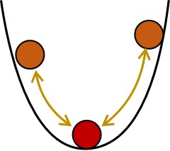
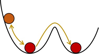
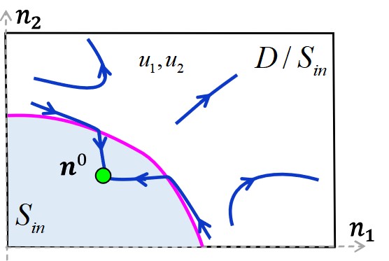
Resilience, first proposed by Holling (1973) in the ecology field, denotes the system ability to absorb unexpected disturbances and to keep persistence. Over the past few decades, resilience has been greatly developed in various disciplines including ecology, engineering, and psychology (Martin-Breen and Anderies (2011), Hosseini, Barker, and Ramirez-Marquez (2016a)). In general, there are two perspectives on resilience: engineering resilience and ecological resilience (Holling (1996)). Noteworthy, this categorization of resilience is discipline-independent. One can use ball-and-cup heuristic to illustrate these two perspectives (Scheffer et al. (1993), Rölfer, Celliers, and Abson (2022), Liao (2012), Walker et al. (2004)), as shown in Fig. 1: when the ball is at the cup bottom, it symbolizes a steady state, known as an “attractor”; the shape of the cup portrays the recoverable phase space of the corresponding attractor, usually described as the shape of potential function (landscape) or attraction basin; the yellow arrows represent perturbations and system responses. Fig. 1(a) illustrates the engineering resilience, which usually assumes there exists a single steady state and characterizes the system ability to absorb disturbances and recover to this single steady state. Studies related to engineering resilience typically aim at rapid local or global recovery of a single steady-state system (Tilman and Downing (1994), O’Neill et al. (1986), Pimm (1984)). In contrast, Fig. 1(b) shows the ecological resilience, which features multiple metastable states and the perturbations are absorbed through a multi-state shifting, without requiring the returning to a single steady state. Clearly, ecological resilience emphasizes persistence with uncertainty (Holling (1973), Folke (2006), Zeng et al. (2022)). As such, ecological resilience can transform a system under instability from one basin of attraction to another (Holling (1973)), even for cases where they are far from the stable equilibrium as defined otherwise in engineering resilience.
Road network resilience is an emerging research subject. Most of the developed works are towards engineering resilience, aiming at a rapid recovery to a non-congested equilibrium or a single optimal equilibrium. For example, the classic perimeter control schemes developed based on the macroscopic fundamental diagram (short for MFD) characterization of congestion dynamics, have received much attention in recent years (Geroliminis and Daganzo (2008), Haddad and Geroliminis (2012), Aghamohammadi and Laval (2020), Laval, Leclercq, and Chiabaut (2017), Johari et al. (2021), Haddad (2015), Khwais and Haddad (2022), Haddad and Zheng (2020), Mariotte, Leclercq, and Laval (2017), Haddad and Mirkin (2020), Ramezani, Haddad, and Geroliminis (2015), Li, Yildirimoglu, and Ramezani (2021), Mohajerpoor, Cai, and Ramezani (2023), Kouvelas, Saeedmanesh, and Geroliminis (2023), Tsitsokas, Kouvelas, and Geroliminis (2023), Yang, Menendez, and Zheng (2019), Dantsuji, Fukuda, and Zheng (2021), Ampountolas, Zheng, and Geroliminis (2017), Yang, Zheng, and Menendez (2018), Su et al. (2020)). The perimeter control schemes regulate the proportion of entering traffic at the perimeter of the networks via traffic signal control. In this direction, Haddad and Geroliminis (2012) calculated the "region of attraction" (short for RA) and designed a state feedback control to increase the RA for enlarging the recoverable area towards a single non-congested stable equilibrium. One pre-condition though, is that the system is within the states as defined by RA. In face of the so-called “hyper-congestion” which is far beyond the stable equilibrium state (e.g. a congestion density value twice as much as the critical density) and beyond RA, recovering to the desired system equilibrium cannot be guaranteed, and the system will inevitably fail, e.g. becoming unrecoverable grid lock. On the other hand, Zhong et al. (Zhong et al. (2020a, 2018a, 2018b)) and Huang et al. (Huang et al. (2020b)) developed control schemes where the control would aim at a designated point, for example the point near the critical density or critical accumulation where the network flow reaches its maximum. However, the sufficient conditions of these controllers require that the disturbance to the systems, i.e. the incoming traffic demand to the road networks, cannot be high and fast-varying over time, which limits the controllability towards real world traffic situations. Most recently, Gao et al. (2022) proposed a novel control scheme based on RA, denoted as RCS-single, focusing specifically towards the recovery to the single optimal equilibrium from hyper-congested states. This is one of the first exploratory works looking at the “resilience” of system control. Nevertheless, this work was still within the framework of a single equilibrium system, and the recovery speed is very slow. For systems where instability is coupled with complex disturbances, in the case of hyper-congestions accompanied by persistently high travel demand, the existing controls are not only time-consuming, but also the objective of returning to single equilibrium is impractical. In literature, the impact of large changes in travel demand causing the instability of MFD was pointed out in multiple studies, such as Daganzo, Gayah, and Gonzales (2011), Zhong et al. (2020b), Haddad and Zheng (2020).
Urban traffic is a complex dynamic system, which may exist multiple metastable states (Zeng et al. (2020)). Given the above discussion on the limitation of the single-objective control schemes, a more realistic way appears to be guiding the system to switch between multiple metastable states under perturbations. While the engineering resilience-oriented system controls have its values, there is a need to address the limitation towards system perturbations. Future resilient traffic system, that is capable of withstanding large and rapidly changing environments and contingencies, absorbing environmental uncertainties and developing different adaptive landscapes, would be by nature an ecosystem-like dynamic system. In other words, controlling such system should embrace an ecological perspective, where the ecological operation essentially enables the system to shift among alternative stable states (Holling (1996), Folke et al. (2010), Walker and Salt (2012), Gunderson (2000), Dakos and Kéfi (2022), Scoones et al. (2020)). Therefore, this work develops an ecological resilience control for managing congested urban road systems. The control aim is to enhance road traffic flow systems with greater adaptability towards different perturbations, such as congestion, unusual travel demand, sudden infrastructure closure, and accidents. Our work will, for the first time, provide an analytical modeling framework and the proves on system shifting between alternative steady states. Our work will demonstrate that such system is superior and much more resilient, comparing to controlled systems that aiming at returning to a single state, such as an original equilibrium or a pre-defined optimal state.
Built upon the MFD-based traffic flow representation system, this paper proposes a methodology for deriving ecological resilience control under large disturbances. Our control methodology comprises three aspects: portraying the recoverable system states, designing the target steady system states, and developing control mechanisms to regulate system towards steady states. Specifically, the RA framework will be adopted but extended, where the recoverable scopes are portrayed by attraction region; the alternative steady states are set close the optimal state and outside the attraction region of the original equilibrium; the controller is devised to guarantee the local stability of the alternative steady states, without changing the dynamics around the original equilibrium as much as possible. We showcase the proposed methodology in two-region road systems (i.e. two congested road networks whose traffic flow and congestion interact with each other, and each road network has its own MFD to describe its traffic dynamics). We first derive the explicit algebraic expressions of the boundaries of inner and outer estimations of the attraction regions. Building upon these theoretical boundary delineations, we then design two distinct resilience control schemes, denoted as RCS-1 and RCS-2, respectively. Considering a four-equilibria system as an illustration, we test two resilient control schemes. The control performance can be seen in Fig. 13 and Fig. 15 (more details and discussions will be provided in section 5). CPC (denotes constant perimeter control) and RCS-single (proposed by Gao et al. (2022)) are two benchmark methods. As a general remark, the proposed resilience control schemes and RCS-single can prevent the evolution of vehicle density (also called vehicle accumulation) or to jam vehicle density (corresponding to zero completion flow), while CPC is unable to impede such occurrences. Furthermore, the resilience measures summarized in Table 2 indicate that, RCS-1 and RCS-2 outperform RCS-single as they exhibit greater resilience measures in most cases, corresponding to smaller resilience triangle (resilience loss). This superiority stems from the ability of RCS-1 and RCS-2 to guide the trajectories towards alternative stable states that are more easily attainable, thereby enhancing adaptability. Moreover, the local landscape (local Lyapunov function (Wang et al. (2021), Willems (1971), Blanchini (1995))) near the target point of controlled system with RCS-2 clearly shows the effect of our control scheme.
The main contributions of this study encompass three key aspects:
-
(1)
We establish a theoretical foundation for the approximate depiction of recoverable states for multi-equilibrium systems, by deriving the inner and outer estimations of attraction regions with explicit algebraic expressions for multi-equilibrium MFD dynamics, utilizing invariant sets. Note that the computation of RA for multiple equilibria nonlinear systems is especially intricate and hard to obtain.
-
(2)
We innovatively propose a leap from single-steady state control (from an engineering resilience perspective) to multi-steady states control (from an ecological resilience perspective), by leveraging the developed theory of approximate depiction of recoverable states and the stability theory of switch systems. This effort yields explicit control methodological, providing a clear pathway for the implementation of a control system that navigates across different stability landscapes.
-
(3)
We innovatively design a resilience measure utilizing the classical resilience triangle and completion flow. And it intuitively depicts the loss of completed trips compared to the maximum potential number of trips that could have been completed during the recovery period.
2 The control system dynamics and its ecological resilience
This paper showcases the advancement and performance of an ecological resilience-oriented control in a two-region system (known also as two-reservoir system in literature) traffic flow control problem, where the traffic dynamics of the two regions follow an MFD-based representation. Sec. 2.1 firstly gives the mathematical description of the MFD-based modeling framework, Sec. 2.2 illustrates the ecological resilience control framework for MFD dynamics, and then Sec. 2.3 defines ecological resilience measure.
2.1 Two-region MFD dynamics
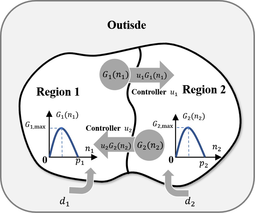
To start with, we consider a two-region MFD system, illustrated in Fig. 2. The urban traffic network is partitioned into three parts: Region 1, Region 2, and the Outside. Our primary focus lies on Regions 1 and 2, and each endowed with its own MFD. The MFD delineates the correlation between the travel completion flow and vehicle accumulation (density) of region at time , manifesting a single peak, characterized by an initial ascent succeeded by a descent. Classical perimeter control methodologies regulate the traffic flow ratio entering Regions 2 and 1 through signal controls, denoted as allowed pass rates and . As illustrated in Fig. 2, for each region at time , there are two inflows (marked as gray arrows directed toward region i) and one completion flow (marked as gray circle). The first inflow, (, ) signifies the allowed traffic inflow transferred from to i with the pass rate . The second inflow, denoted as , represents the fixed net inflow from the outside to , encapsulating uncontrollable demand, commonly known as disturbance.
The model can be described by MFD dynamic (Aboudolas and Geroliminis (2013), Gao et al. (2022)):
| (1) |
with the boundary condition:
| (2) |
Let , , and , system (1) can be simplified to . Note that perimeter controllers and are assumed to be constants. Therefore, they can be denoted as constant perimeter control, short for CPC. The fixed net inflow is also assumed to be constants. Moreover, as a realistic scene, we here use the parabolic-MFD: with opening size and jam accumulation of region , as shown in Fig. 2 and Fig. 3. Then we have the maximum capacity at the critical vehicle accumulation . Note that , and are satisfied to avoid overflow. Without loss of generality, we can assume , then the condition of and in Eq. (2) can be simplified as Condition :
| (3) |
For the two-region MFD dynamic (1) with boundary condition (2) under traffic demand , given the MFD function , we aim to generate a transportation system from ecological resilience perspective by combining the stability characteristics of the MFD dynamics.
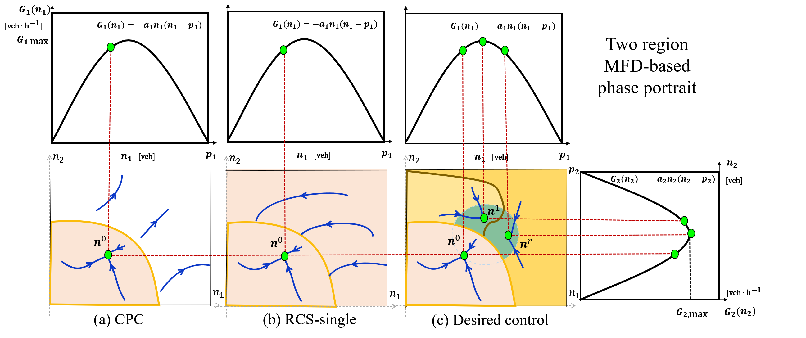
To achieve this objective, we first introduce concepts related to stability characteristics. The stability characteristics can be elucidated by phase portrait, where the phase portrait is a geometric representation of the dynamic system trajectories on the phase plane. As shown in Fig. 3(a), the phase plane is , and each point (state) in plane denotes the vehicle accumulation in two regions. Progressing to the right or upward along the plane signifies a corresponding increase in the vehicle accumulation within Region 1 (Region 2). Moreover, the axis in Fig. 3(a) corresponds to the ordinate of the right MFD and axis corresponds to the abscissa of the upper MFD. The completion flow () increases with the vehicle accumulation before the critical vehicle accumulation (), reaching a peak (), and subsequently decreases until it diminishes to zero at the right (upper) boundary, signifying a traffic jam. As shown in Fig. 3(a), the attraction region (light pink region) of the equilibrium point (green circle) is a set of the initial points. The trajectories start from these initial points will converge towards , while trajectories start from outside attraction region will move away from and towards either the upper or right boundary. Note that equilibrium point satisfies . We can introduce the definition of attraction region for the general equilibrium as follows:
Definition 2.1
Note that, the classical concept of the "attraction domain" was originally defined for asymptotically stable equilibria (Wang, She, and Ge (2020b), Zheng et al. (2018), Ratschan and She (2010), Wang, She, and Ge (2020a)). Especially, for MFD dynamic (1), Gao et al. (2022) defined the "attraction region" for the unstable single equilibrium point. Differently, we here in this paper define for the general equilibrium , including both unstable equilibrium and stable equilibrium.
2.2 Ecological resilience control framework for MFD dynamics
In the traffic flow theory and traffic control community, how to recover the traffic system from congestion has been a challenging research question. The classical perimeter control schemes, which utilizes MFD as references for optimal control, target on recovering the traffic system to a specified equilibrium. Such schemes are known to be constrained and uneconomical for hyper-congestion conditions, because these conditions are far from the single optimal control objective and there exist complex dynamics in the system that prevent the system from even getting closer to the targeted equilibrium. For this reason, our approach defines a new control objective, built upon which a corresponding control methodology is developed.
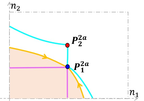
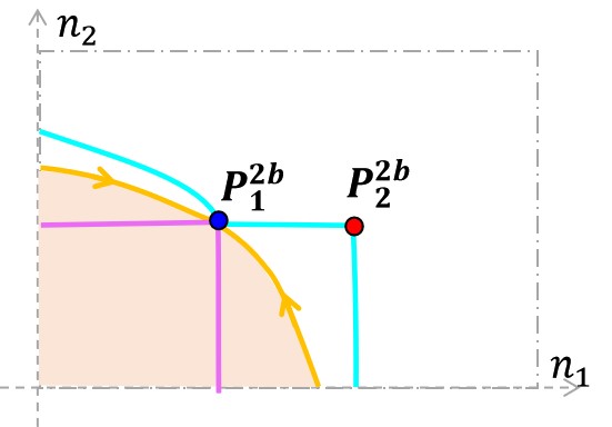
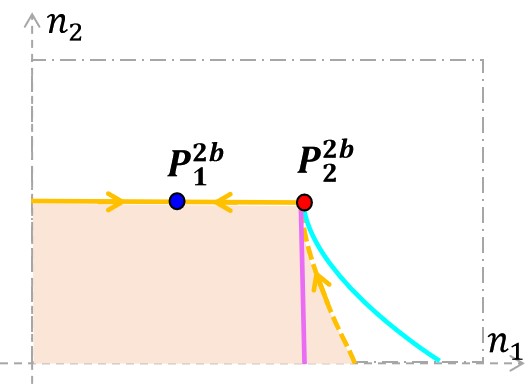
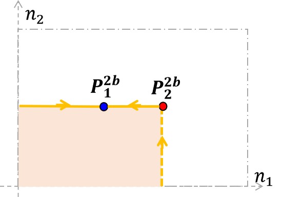
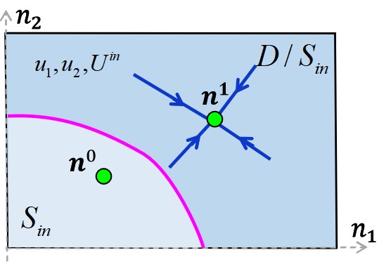
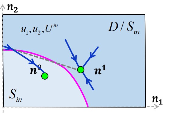
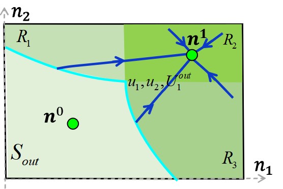
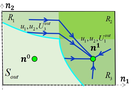
In essence, ecological resilience considers the existence of multiple metastable states in a dynamic system, and it enables the system to shift between states as a way to absorb or adapt to rapid external changes. Inspired by this nature, we aim to construct an ecological resilience traffic system resembling Fig. 3(c), with multiple metastable states (marked as green circles), where multiple metastable states includes the original uncongested equilibrium and alternative steady states ( with number of alternative steady states ).
To generate the ecological resilience traffic system resembling Fig. 3(c), our first critical issue is how to select multiple metastable states. Initially, we aim to leverage the inherent landscape of the system as much as possible. Therefore, we preserve the original non-congested equilibrium point of the system, denoted as . This point coincidentally aligns with the single equilibrium point set by the classical CPC control system (as shown in Fig. 3(a)) or the single equilibrium point of the RCS-single control system proposed by Gao et al. (2022) (as depicted in Fig. 3(b)), satisfying . After determining , the next step involves selecting alternative stable states . There are two key criteria for selecting alternative stable states: one to position them as close to the optimal and critical vehicle accumulation as possible; the other is to position them outside the attraction region (depicted in the light pink region) of the original non-congested equilibrium point . The first criterion seeks to increase the completion flow, given that such completion flow tends to decline as the vehicle accumulation gets further from the critical vehicle accumulation (see Fig. 3(c)). The second criterion is crucial because states within the attraction region of will spontaneously recover to . Here, we provide a quantitative description of the selectable range. For the first criterion, we aim to select , such that the absolute distance between completion flow and maximum completion flow is less than , where denotes the absolute distance between completion flow of the original equilibrium and maximum completion flow. That is,
| (5) |
substituting and , yields
| (6) |
corresponds to the interior of an ellipse. Combining the second criterion, the selectable range of alternative stable states is
| (7) |
as the green region shown in Fig. 3(c).
Once multiple metastable states have been chosen, the next consideration is how to devise a control scheme that enables the system to recover to appropriate steady states. Controlling a system with multi-steady states poses more challenges compared to a system with a single stable state. The first challenge lies in determining which state the system should recover to, and the second challenge is devising a strategy to facilitate the system recovery to the respective target stable state. To address the first challenge, we need to identify the attraction region of the original equilibrium. It is essential to note that, for nonlinear systems, the attraction region is typically intricate, and obtaining explicit algebraic expressions for it can be challenging. In this direction, Gao et al. (2022) derived the attraction region with explicit algebraic expressions for the single-equilibrium MFD dynamics. Different from their work, we consider multi-equilibria (including two-equilibria and four-equilibria) systems in this paper. Given the involvement of multiple equilibrium points and nontrivial boundary shapes, their approach can not be applicable here. To this end, our first effort is the estimation of the attraction region for the multi-equilibria systems (see Sec. 3 and App. 7). Upon obtaining an estimation of the attraction region with explicit expressions for the boundaries (including inner and outer estimations) of the original uncongested equilibrium point, a natural boundary between the original uncogested equilibrium and the alternative steady state emerges.
The second challenge, i.e., how to devise a strategy to facilitate the system recovery to the respective target steady state is also intricate. To tackle this issue, we make a second effort using a switched controlled system and design two control schemes based on the inner and outer estimations of the attraction region (see Sec. 4). It is essential to emphasize that Gao et al. (2022) also explored this direction. Their switched controlled system is depicted in Fig. 3(b), where trajectories originating outside the attraction region are directed towards its boundary before spontaneously converging towards the single equilibrium. The proposed control, however, addresses a significantly different and more complex problem. We aim to utilize the escaped trajectories (from attraction region) and guide them to appropriate steady points. Therefore, this novel framework faces new technical barriers, namely how to find a feasible control that can recover system to of target point within recovery time under corresponding perturbations, where denotes an arbitrarily small positive number; and of a state is described as the set . Note that the target point can be any state in multiple metastable states, depending on the size of the perturbation; and system can switch between multiple metastable states in facing with different perturbations. Moreover, the system can also switch between optimal and suboptimal states, if the optimal state satisfies the conditions of the alternative steady states.
2.3 Measuring urban traffic resilience
We have depicted the envisioned ecological traffic resilience system and presented the resilience control framework. However, a quantitative indicator for traffic ecological resilience is still absent. It is imperative to establish a quantitative measure for traffic ecological resilience, thereby enhancing a more intuitive perception of the ecological resilience of traffic and facilitating a more straightforward evaluation and reference for control effectiveness.
The quantitative assessment of resilience can be categorized into two main types: general resilience measure methods and structure-based model-driven resilience measure (Hosseini, Barker, and Ramirez-Marquez (2016b)). We prioritize general resilience measure in this paper, given that the second type is more reliant on specific models. Among general resilience measure, the “resilience triangle” introduced in Bruneau et al. (2003) has gained notable attention. Originally designed for assessing a community resilience loss during earthquakes, it calculates the resilience loss through a definite integral:
| (8) |
where represents community service quality at time , expressed as a percentage scale from 0 to 100. starts declining at and returns to the normal state at . The deviation between the quality of degraded infrastructure and the normal infrastructure quality is quantified through . A higher RL indicates lower resilience, while a lower RL suggests higher resilience.
In this direction, Gao et al. (2022) marks one of the initial attempts to provide a quantitative interpretation of urban traffic resilience. They defined urban traffic resilience as the integral of the absolute deviation between vehicle density (vehicle accumulation) and the optimal vehicle density during the recovery period. However, the defined resilience measure lacks an evident physical interpretation. Thus, we revise the definition of deviation as the difference between the completion flow and the maximum completion flow . That is:
| (9) |
Note that, the unit of is . Based on the defined , we can define the ecological traffic resilience measure as follows:
| (10) |
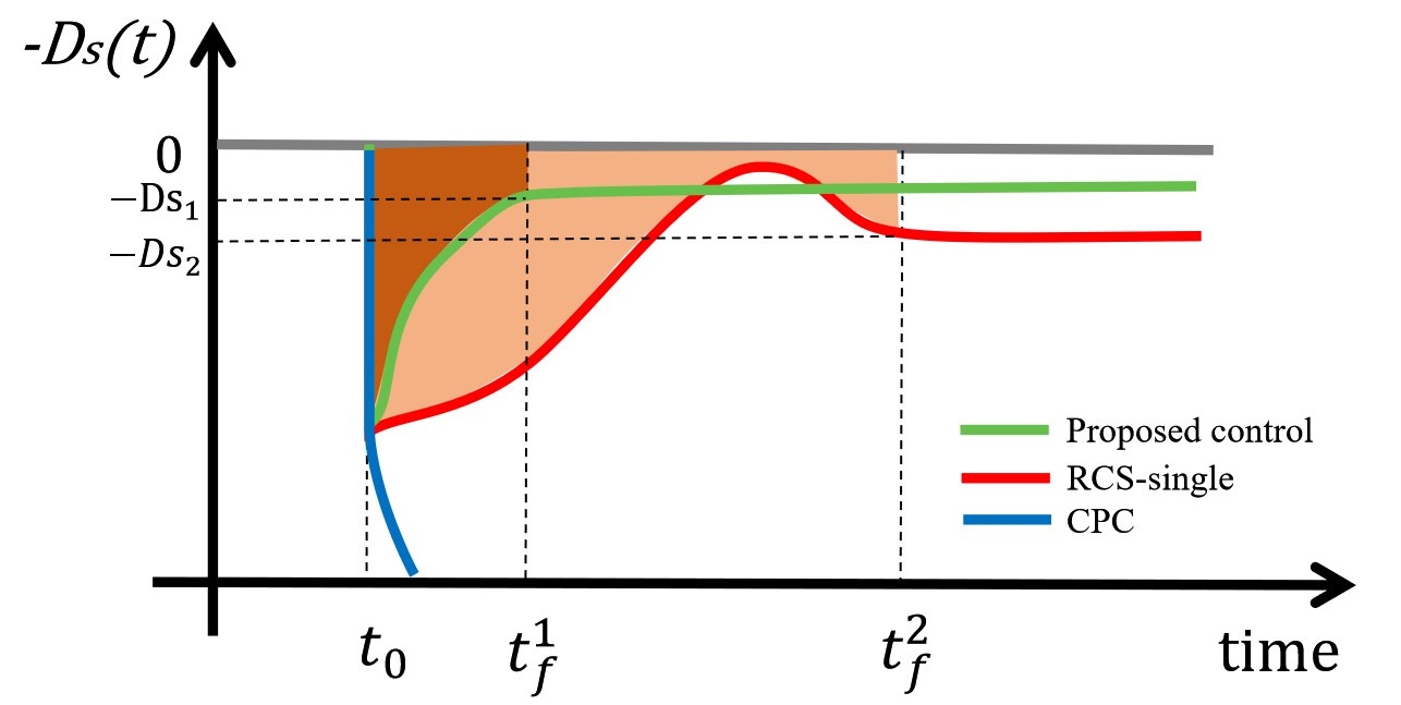
Here is the time when system recovers and stabilizes at functional steady states. Formula (10) implies that is negative. Thus, corresponds to the area of the resilience triangle, depicted as the dark brown shaded region in 4. Noteworthily, the unit of resilience measure is , and it denotes the loss of completed trips compared to the maximum potential number of trips that could have been completed during the recovery period.
We depict a schematic diagram of the resilience triangle under three different controls, as shown in Fig. 4. Notably, under hyper-congestion, CPC fails to recover system and instead rapidly collapses system; while RCS-single and the proposed control can ensure recoverability. The resilience control proposed in this paper outperforms RCS-single, as it enables the system to recover to an alternative stable states with higher completion flow within a shorter time. Thus, the resilience triangle (loss) under our proposed control method (the dark brown area in Fig. 4) is smaller than that of RCS-single (the light brown area). Note that the original equilibrium is assumed to be a stable non-congested state, rather than an optimal state.
3 Stability analysis and spontaneous attraction region estimation for multi-equilibria system
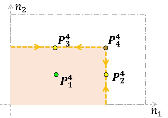
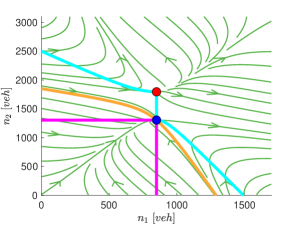
In the previous section, for multi-equilibria system, we defined ecological resilience of urban traffic with an MFD-based representation. In this section, we will derive the global phase portrait and the spontaneous attraction region for the multi-equilibria system under CPC ( and ). Sec. 3.1 discusses and verifies the local stability of the MFD dynamic; Sec. 3.2 derives and illustrates the global phase portrait; and Sec. 3.3 presents the estimation of spontaneous attraction region that are used to design the proposed control in Sec. 4. Note that multiple equilibria systems include both two-equilibrium systems and four-equilibrium systems. According to Gao et al. (2022), two equilibria exist if and only if Condition : or Condition : holds; four equilibria exist if and only if Condition : holds. We in this section mainly present the theoretical analysis for two-equilibria system. The theoretical analysis for four-equilibria system can be found in App 7.
3.1 Local stability verification
Consider the two-equilibria case with Condition . According to Condition , we have:
| (11) |
Bringing the first equation of (11) into system (1), the system dynamics become:
| (12) |
For systems (3.1), the two equilibria can be denoted as (), where , . Upon substituting Formula (11) into Formula (1), the system (1) reduces by one variable, , significantly simplifying our analysis. However, Formula (3.1) remains cumbersome. To further simplify the system for subsequent analysis, we shift equilibrium point of the system (3.1) to . That is, letting and , we can simplify system (3.1) as:
| (13) |
The two equilibria for the new system (3.1) are and . Noteworthy, system (3.1) possesses the same properties as system (3.1) since system (3.1) is obtained by shifting system (3.1). Due to the simpler formulation of system (3.1), we in the following use system (3.1) to derive local stability characteristics, global phase portraits, and attraction region estimations. The properties obtained are equally valid for system (3.1). Therefore, all our propositions and theorems are summarized for system (3.1).
From the aforementioned conversion, we derive the following proposition for its two equilibria.
Proposition 3.1
Under Condition , the two equilibria and of system (3.1) are both saddle-node points.
Proof: We have that and of system (3.1) are equivalent to and of system (3.1), thus we consider the stability of and . For , we have , indicating that:
and
According to Theorem 7.1 in Zhang (2006), we can analyze the nature of equilibrium points by calculating the bifurcation function (defined in Zhang (2006)), yields:
where is obtained by letting . Since Condition holds, we have holds for all except . Moreover, the power exponent of function is 2. Thus, is a saddle-node point (see Zhang (2006) Theorem 7.1(iii)), indicating that is a saddle-node point. Similarly, we can prove that is a saddle-node point.
Proposition 3.1 reveals that, for system (1) under , the two equilibria and are both saddle-node point. Similarly, for system (1) under , we can also prove that two equilibria and are both saddle-node point. These results will help us to reveal the local stability of the two equilibria, which will assist in subsequent derivations of attraction region, providing foundation for understanding the global properties of the system.
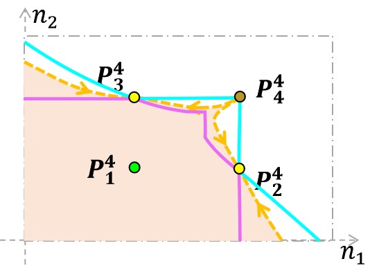
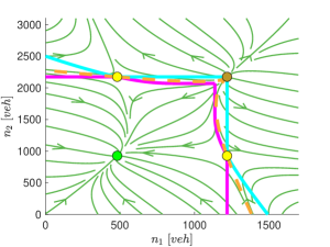
For the four-equilibria system, we also try to capture the local stability through linearization, and the detailed analysis can be found in App. 7.1. In App. 7.1, we denote the four equilibria as (), and we have that is a locally stable node, and are saddle points, is an unstable node, which can be summarized as Proposition 7.1 in App. 7.1.
3.2 Global phase portrait derivation
To capture more properties of the system, we aim to delve further into its global nature. Global analysis of dynamical systems is often intricate, lacking a unified analytical approach. For MFD dynamics, we overcome this gap by first dividing the phase space into several subregions using demarcation lines, followed by delineating the trajectory trends within each subregion, and ultimately analyzing and deriving the global phase portrait leveraging the trajectory trends in each subregion. For simplicity in analysis, we continue to consider the more straightforward formulation of Formula (3.1). Note that, the aforementioned demarcation lines are obtained by solving =0 or =0 respectively. The trajectory trends in each region are determined by and . For instance, if > 0 (> 0), the trajectories move to the right (upward), while if < 0 (< 0), the trajectories move to the left (downward). Furthermore, considering that the demarcation lines =0 or =0 take different shapes under four distinct parameter conditions, we will separately examine these under four conditions.
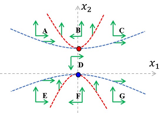
First consider Condition : . Under this condition, both demarcation lines manifest as hyperbolas, illustrated by the red and blue dotted curves in Fig. 5(a), with the expressions and . In addition, we have and on the red dotted curves except for and ; and we have and on the blue dotted curves except for and . It is worth mentioning that, since holds, the location of these four curves are is uniquely determined, as shown in Fig. 5(a). Then, the plane can be divided into seven unbounded regions by these four curves. Moreover, Table 1 summarizes the symbols of () in these seven regions. On the basis of Table 1, the phase portrait of (3.1) under Condition can be obtained, as shown in Fig. 5(a).
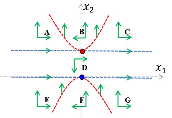
| Derivative | Symbol in region | ||||||
| A | B | C | D | E | F | G | |
Subsequently, we can verify that regions B and E are both positive invariant sets by utilizing proof by contradiction. Given that the trajectories starting from B and E will not escape, we can further obtain that there exist no close orbits for system (3.1) under Condition .
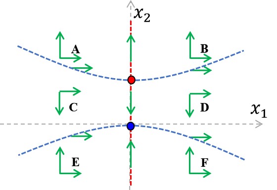
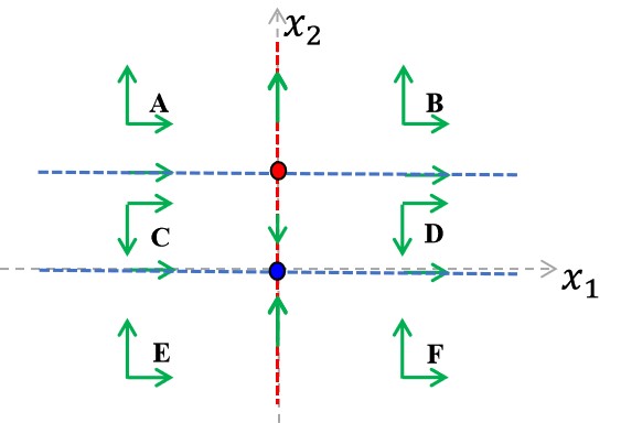
When Condition : , : or : hold, the two demarcation lines can manifest as one hyperbola and one straight line (as shown in Fig. 5(b) and 5(c)) or as two straight lines (as shown in Fig. 5(d)). After obtaining the demarcation lines, we follow similar steps as above. As such, we verify that no close orbits exist under these conditions, and the corresponding phase portraits are illustrated in Fig. 5(b), 5(c) and 5(d). Similarly, we can also obtain the phase portrait for system (1) under Condition , and there also exists no close orbit.
For the four-equilibria system, we also try to capture the global phase portraits, and the detailed analysis can be found in App. 7.2. Note that the steps of global phase portrait derivation differ from that used for two-equilibrium system. Due to the increased number of equilibria, the combination of demarcation lines becomes intricately complex. On one hand, variations in demarcation line types (e.g., two hyperbolas, one hyperbola and one straight line, two straight lines, etc.) lead to different phase portraits. On the other hand, different relative positions of demarcation lines (e.g., whether the foci of two hyperbolas lie on the same axis) add another layer of complexity. The method for two equilibria are insufficient to address the challenges posed by four equilibria. Furthermore, the increased number of equilibrium points also hinders us from directly determining the locations of corresponding separatrices. New methods are required to capture the global phase portrait. We solve these in App. 7.2 by subdividing Condition into five new distinct conditions. That is, Condition : ; Condition : ; Condition : ; Condition : ; Condition : , where ; and . The five conditions mentioned above correspond to different positions of demarcation lines. In App. 7.2, by discussing the shape of critical demarcation lines under each condition, we have summarized 20 distinct phase portraits for four-equilibria system and verifies that no closed orbit exists.
3.3 Spontaneous attraction region estimation
In the following, for two-equilibria system (3.1), the attraction region for the unstable saddle-node point will be derived. Note that, Gao et al. (2022) developed a method to find certain special trajectories, e.g., for system with single-equilibrium. This form of special solution cannot apply here for multi-equilibrium systems. In this case, the theoretical attraction region boundaries are identified by finding certain separatrices of the equivalent systems (3.1), and the inner and outer attraction regions can be obtained by finding the positive invariant sets, under the aforementioned four conditions respectively.
Firstly, we consider Condition . As shown in Fig. 6(a), the two red dotted demarcation curves can be denoted as (), where . Similarly, the two blue dotted demarcation lines can be denoted as (), where . Obviously, the vertexes of the demarcation lines are exactly the two equilibria and .
Assuming the lower blue dotted line intersects with at and , where . The trajectory starting from and will go into in E as ; and the trajectory starting from will escape A from the upper boundary of A and stay in B moving away from as . Thus, due to the continuous dependence theorem of solutions on initial conditions (Zhang (2006)), there exists a with , such that the trajectory starting from any with will enter E and then go to in E as , and the trajectory starting from any with will enter A, then escape A from the upper boundary of A and stay in B moving away from as . Thus, the trajectory starting from , donated as = , is a stable separatrix of , as shown in Fig. 6(a). Similarly, assuming the lower red dotted line intersect with at and . By similar analysis, we can obtain that there exists an with , such that the trajectory starting from any with will enter E and then go to in E as , and the trajectory starting from any with will enter G, then escape G from the upper boundary of G and stay in D moving away from as . Thus, the trajectory starting from , donated as , is a stable separatrix of , as shown in Fig. 6(a).
Subsequently, combining with phase portrait Fig. 5(a), we can verify that the region is a positive invariant set utilizing proof by contradiction, where , depicted as the light blue zone in Fig. 6(a). Or else, there will be at least one trajectory originated from , and enter (or ) through the upper boundary (or right boundary) of , where and . Obviously, it is contradictory with the trajectory direction in phase portrait 5(a). Further, joining Fig. 6(a) with Fig. 5(a), we have that: the trajectory starting from any point in will escape D from the lower boundary of D and entering E, and the trajectory starting from any point in will escape F from the left boundary of F and entering E. Since E is a positive invariant set, and we have and in E, the trajectory starting from any point in E will go to as . Thus, the trajectory starting from any point in the positive invariant set will go to as , implying , i.e., is an inner estimation of attraction region (Zheng et al. (2018), Wang, She, and Ge (2020b)) for .
Similarly, region (the light yellow region shown in Fig. 6(a)) is also a positive invariant set, where
Note that and are also positive invariant sets. In addition, the trajectory starting from point in will escape from the upper boundary of and enter moving far from , or escape from the lower boundary of and enter moving far from . Thus, we can obtain that , i.e., the region is an outer estimation of attraction region for . Further, we can obtain that and , as the yellow lines shown in Fig. 6(a).
When Condition hold, we can obtain two stable separatrices and of ; the inner estimation of attraction region ; and outer estimation of attraction region by similar analysis. Furthermore, we have and , as shown in Figs. 6(b). When or hold, we can first simplify the system (3.1) by bringing in corresponding conditions. Then, by repeating the above analysis, we can obtain corresponding results, as shown in Figs. 6(c) and 6(d).
Consequently, for the system (3.1), the estimation of the attraction region for the saddle-node points has been obtained. Further, letting and , the estimation of attraction region for can be obtained. Denoting and , where , we can obtain the theorem as below.
Theorem 3.2
For the unstable saddle-node point , under Condition , we have , where the attraction region , the inner estimation of attraction region and the outer estimation of attraction region are defined as follows:
-
(1)
Under Conditions and , , where and denotes the two stable separatrices and of , respectively;
, where
and
-
(2)
Under Condition , , where denotes the stable separatrix of ; ; ;
-
(3)
Under Condition , .
Note that () holds all the time.
Similarly, for system (1) under Condition , we can obtain the inner () and outer () estimations of attraction regions for under four different conditions, as shown in Fig. 8.
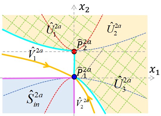
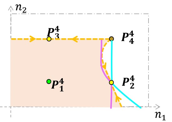
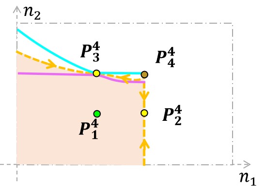
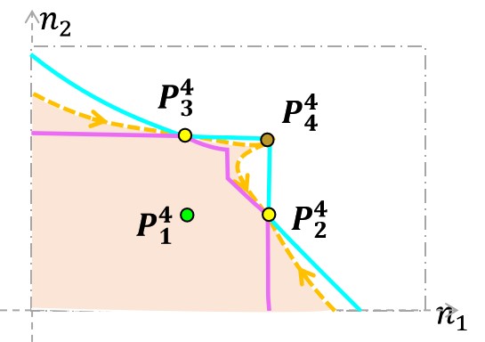
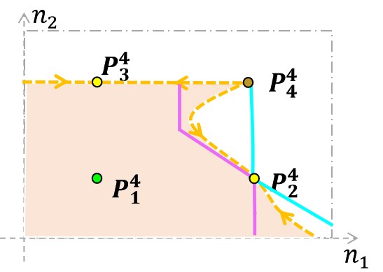
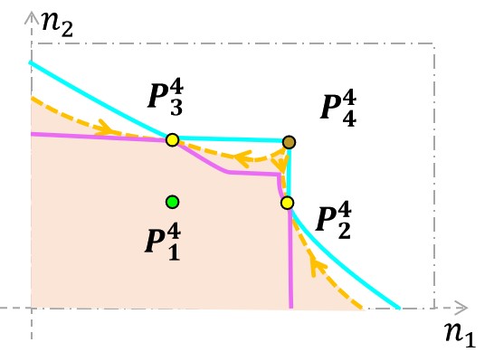
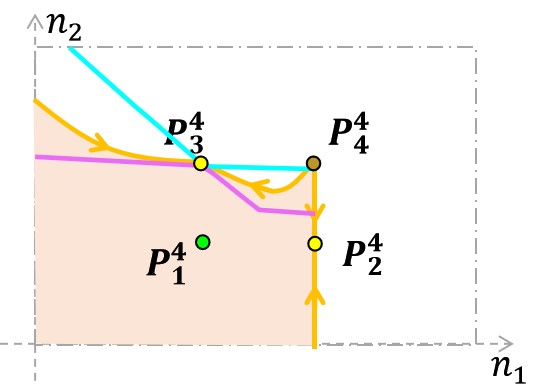
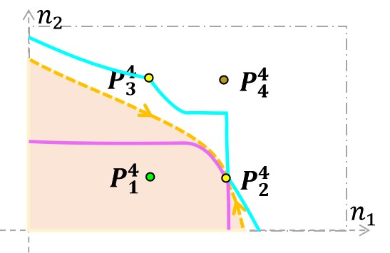
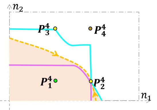
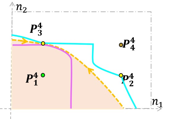
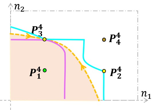
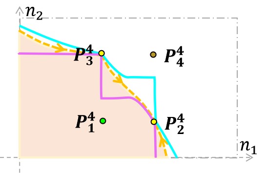
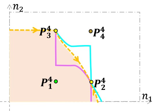
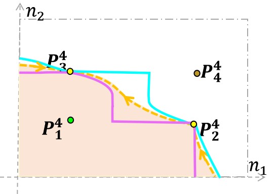
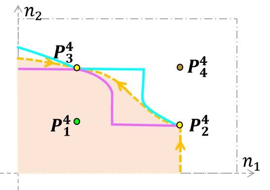
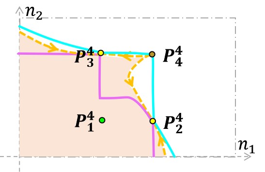
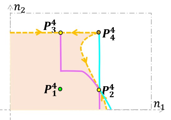
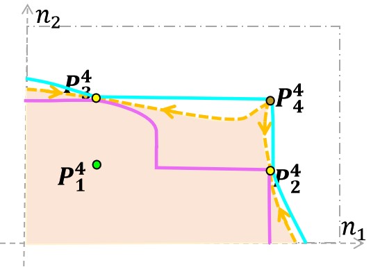
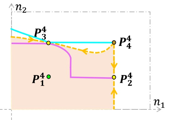
For the four-equilibrium system, we also try to obtain the inner () and outer () estimations of attraction regions, and the detailed analysis can be found in App. 7.3. Note that for the four-equilibrium system, the attraction regions become more intricate due to the increased number of equilibria. In App. 7.3, through a novel classification method, we obtained 20 distinct inner and outer estimations of attraction regions, which can be summarized as Theorems 7.2, 7.3, and 7.4 in App. 7.3. The geometries of the attraction region for the four-equilibrium system are illustrated as the pale pink region shown in Fig. 9.
4 Ecological resilience control design
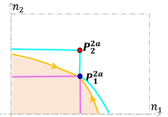
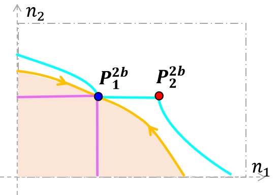
In the previous two sections, we obtain the inner () and outer () estimations of attraction regions with explicit algebraic expressions under each condition for a multi-equilibria MFD-represented traffic dynamic system (1). Note that for two-equilibria system, corresponds to or , and corresponds to or ; for two-equilibria system, corresponds to and corresponds to . While In this section, we will design two distinct resilience control schemes, aiming to facilitate the recoverability of the system to its respective steady states while minimally altering the original landscape, utilizing the obtained and . Sec. 4.1 illustrates the resilience control schemes utilizing , denoted as RCS-1, and Sec. 4.2 provides the resilience control schemes utilizing , denoted as RCS-2.
The trajectories starting from inside attraction region (or inner estimations of attraction regions) can converge to the original equilibrium, while for those that starting from outside attraction region (or outer estimations of attraction regions) will move away from the equilibrium. Our primary task is to control the trajectories that move away from the equilibrium point and guide them towards an alternative steady state. For multi-equilibria systems (1), we set up an alternative steady state = in or , respectively. Then, the control schemes (RCS-1 and RCS-2) shall steer the trajectories to the of within the recovery time . Note that the control does not necessarily bring the system to the equilibrium state , which allows the system to be adaptive (to a feasible steady state) and recoverable (to less congested state progressively).
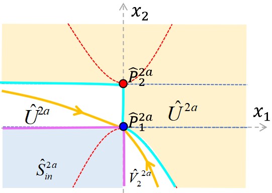
Generally speaking, there are three main differences between the RCS-1 and RCS-2 schemes. With respect to control “intensity”, RCS-1 is more aggressive than RCS-2. That is, the control region for RCS-1 is much larger than RCS-2, as control action () are imposed in () under RCS-1 (RCS-2) and we have . With respect to control mechanism, RCS-1 has a universal control algorithm applied to all alternative steady states, while RCS-2 applies three forms of control, depending on the location of the alternative steady state. Here, we choose three control methods to prevent the emergence of new equilibrium points on the boundary of outer estimation of attraction regions. For instance, trajectories from the boundary of tend to escape , and one control scheme might lead to intersections between trajectories from and trajectories from . This could potentially generate new equilibrium points on the boundary of the outer estimation of attraction regions, complicating theoretical derivations and causing control inefficiencies. With respect to control effect, the trajectories starting from will move towards , while trajectories starting from will move towards (Fig. 10(b)), or (Fig. 10(c)).
4.1 Control formulation of RCS-1
The domain can be divided into two subregions: and , as shown in Fig. 10. If the starting points are in , CPC and that satisfy Conditions , or are conducted. According to Theorems 3.2, 7.2 and 7.4, trajectories from these starting points will move towards the . Instead, if the initial states are in , new control action is activated for recovering trajectories starting from to the of the target point within the recovery time , The target point can be the uncongested equilibrium or the alternative steady state in . Specifically, for system (1), if the starting states are in , we apply the following control , defined by:
| (14) |
where . By adding proposed controller (14) to system (1), the trajectories starting from will move towards directly (Fig. 10(b)), or intersect (Fig. 10(c)). Once intersecting , we rest the control, i.e., immediately, as such that the trajectories will follow the initial system (1). According to Theorems 3.2, 7.2 and 7.4, trajectories from these starting points will move towards the .
By doing so, we have developed a switched controlled system (She and Xue (2014), Skafidas et al. (1999), Gao et al. (2022), She et al. (2020)) as:
where when , when .
Remark 4.1
For multi-equilibria systems (1), certain inner estimations of attraction regions do not contain its partial boundaries (e.g. Figs. 6(d), 8(d), 9(b) etc.). This is because the trajectories starting from the partial boundaries will deviate from the uncongested equilibrium point. In such cases, are imposed until the trajectories intersect with , where is obtained by moving the line down (or left) by .
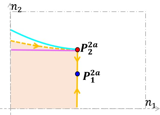
4.2 Control formulation of RCS-2
RCS-2 is designed based on . Likewise, the domain can be divided into and , and can be further divided into , and , as illustrated in Fig. 11. If the starting states are in , CPC and that satisfy Conditions , or will be conducted. According to Theorems 3.2, 7.2 and 7.4, trajectories from these starting points will move towards or escape from the upper boundaries of and enter . Once the states enter in , control action will be activated for recovering trajectories to the of in within the recovery time .
Specifically, for a given system (1), there are three cases of control action , depending on the location of . First consider Case 1, where lies in , as depicted in Fig. 11(b). In this case, proposed RCS-2 is as follows: in addition to and , we will apply an additional control in , and in , where are defined by:
| (15) |
and are defined by:
| (16) |
by adding proposed controller (4.2) to system (1), the trajectories starting from will vertically escape from the upper boundary of and enter . Moreover, by adding proposed controller (15) to system (1), the trajectories starting from will move towards directly, as shown in Fig. 11(b). Thus, any trajectories entering will move towards under the controller.
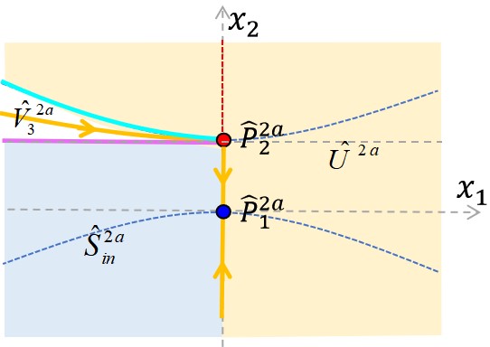
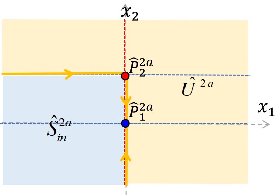
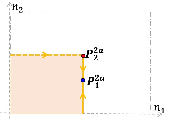
Then consider Case 2, where lies in . In this case, in will be applied. Subsequently, any trajectories going into will go to under our proposed controller, as shown in Fig. 11(c).
Finally consider Case 3, where lies in , as shown in Fig. 11(d). similarly, we will apply control action in , and in , where are defined by:
| (17) |
by adding proposed controller (4.2) to system (1), the trajectories starting from will horizontally escape from the right boundary of and enter . Moreover, by adding proposed controller (15) to system (1), the trajectories starting from will move towards directly, as shown in Fig. 11(d). Thus, any trajectories entering will move towards under our proposed controller.
By doing so, we have developed another switched controlled system (She and Xue (2014), Skafidas et al. (1999), Gao et al. (2022), She et al. (2020)) as:
where when , and features different formulation in different cases when . Specifically,
-
•
in case 1, when and when ;
-
•
in case 2, when ;
-
•
in case 3, when and when .
Remark 4.2
and would have the same formulation if the alternative steady state in both controllers are same. This implies that there may exist initial states, such that the system may end up with identical recovery trajectories under RCS- 1 and RCS-2, respectively.
Furthermore, for a given system (1), if a stable equilibrium point exists (i.e., Condition holds), a local Lyapunov function can be found (Wang et al. (2021), Willems (1971), Blanchini (1995)) for the new controlled system with RCS-2. Specifically, denoting , we can prove that the function is a local Lyapunov function for system (1) with RCS-2, where and
with ; ; . Obviously, holds for all except for and . Moreover, holds if and only if and . In addition, in the neighborhood of , we have holds, and detailed proofs are as follows:
Letting , where , we can transform the system (1) into:
| (18) |
where ; ; and represent second-order remained terms.
By the above coordinate transformation, denoting , we can obtain that:
| (19) | |||||
where and . Then we have:
| (20) | |||||
where represents the high-order remained terms, and the lowest power of it is cubic. Obviously, holds for arbitrary in the neighborhood of except , as we have . That is, holds for arbitrary in the neighborhood of , implying function serves as a local Lyapunov function for the system in the neighbor of .
Similarly, we can prove that holds in the neighborhood of . Specifically, letting and , we have
| (21) |
where represents the high-order remained terms, and the lowest power of it is cubic. Obviously, holds for arbitrary in the neighborhood of except , as is a symmetric positive definite matrix. In other words, holds for arbitrary in the neighborhood of , implying function is also local Lyapunov function for system in the neighbor of .
5 Case studies
In this section, the control performance of the proposed resilient control by comparative case studies are demonstrated. In particular, we benchmark with the classical perimeter control (CPC) and the traffic-resilience oriented control proposed in Gao et al. (2022).
5.1 Numerical verification
A two-region system is set up for case studies, where the network and traffic settings follow the Downtown San Francisco road network from Aboudolas and Geroliminis’ work (Aboudolas and Geroliminis (2013)). We adopt the function form of the MFD models from Gao et al. (2022) for comparison purposes, i.e., for region 1 and for region 2, with maximum capacity , and jam accumulations , .
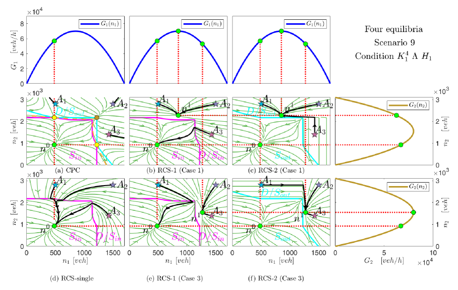
Based on this MFD data, we consider traffic flow dynamics following Eq. (1) and (2) as defined in Sec. 2.1. We first validate the theoretical results of inner and outer estimation of attraction regions for both two and four equilibria derived in Sec. 3 (refer to Theorems 3.2, 7.2 and 7.4, Figs. 7, 8 and 9), accumulating to a total of 28 distinct phase portraits (8 for two-equilibria system and 20 for four-equilibria system). To achieve this, we consider 28 different scenarios, labeled as Scenario 1 to Scenario 28. Each scenario has distinct allowed flow rates and net fixed demand (), corresponding to the 28 conditions in Sec. 3. For example, Scenario 1 corresponds to Condition . We showcase two scenarios (scenario 1 and scenario 9) in Fig. 12. Fig. 12(a) depicts the phase portrait for Scenario 1: , satisfying Condition , corresponding to the two-equilibrium case. It verifies Theorem 1 (or Fig. 7(a)). Fig. 12(b) presents the phase portrait for Scenario 9: , satisfying Condition , corresponding to the four-equilibrium case. It verifies Theorem 2 (or Fig. 9(a)). Parameters and numerical results for other scenarios can be found in App. 8: Fig. 22, Fig. 23 and Table 4. The results are also consistent with our theoretical findings.
Next, numerical phase portraits of the controlled systems under RCS-1 and RCS-2 are demonstrated, as depicted in Fig. 13(b), 13(c), and 13(e), 13(f). Here we use Scenario 9 as a showcase, which corresponds to the complex four-equilibria case. For the simpler two-equilibria case, the control scheme can also be applicable. Note that Case denotes the case where the alternative steady state . The illustration of can be found in Fig. 11. Here, we take Case 1 () and Case 3 () as examples. Fig. 13(a) represents the results under CPC control, serving as a benchmark control. Let us focus on the part in Fig. 13(a), (b), and (e). In Fig. 13(a), a small portion of the trajectories in enters , while a larger portion of the trajectories moves towards the upper or right boundaries of the phase portrait, approaching grid-lock, i.e., high traffic density but low outflow. In contrast, Fig. 13(b) and 13(e) demonstrate that RCS-1 is capable of guiding trajectories starting from towards either the non-congested equilibrium point or the alternative steady state in , avoiding grid-lock. Similarly, in Fig. 13(a), trajectories in all move towards the upper and right boundaries of the phase portrait, while Fig. 13(c) and 13(f) confirm that RCS-2 directs trajectories in towards the alternative steady state in . These results demonstrate the recoverability under RCS-1 and RCS-2. Furthermore, the similar trajectories in (upper region in ) in Fig. 13(b) and 13(c) confirm that there exist some initial states such that the recovery trajectories starting from them under RCS-1 and RCS-2 are identical, as illustrated in Remark 2. This is because, in , RCS-1 and RCS-2 have the same control formulation.
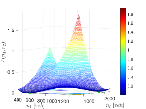
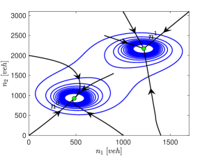
Moreover, for the case where the system has a stable equilibrium (we here use scenario 9 as a showcase), we can find the function defined in Sec. 4.2, as shown in Fig. 14(a), is a local Lyapunov function for the controlled system with RCS-2. Moreover, the projection of in the plane is shown in the Fig. 14(b). Note that the local Lyapunov is only applicable to four-equilibria system, and is not suitable for two-equilibria system, as the there exist no stable equilibria in two-equilibria system.
5.2 Comparison on proposed two control schemes with CPC and RCS-single
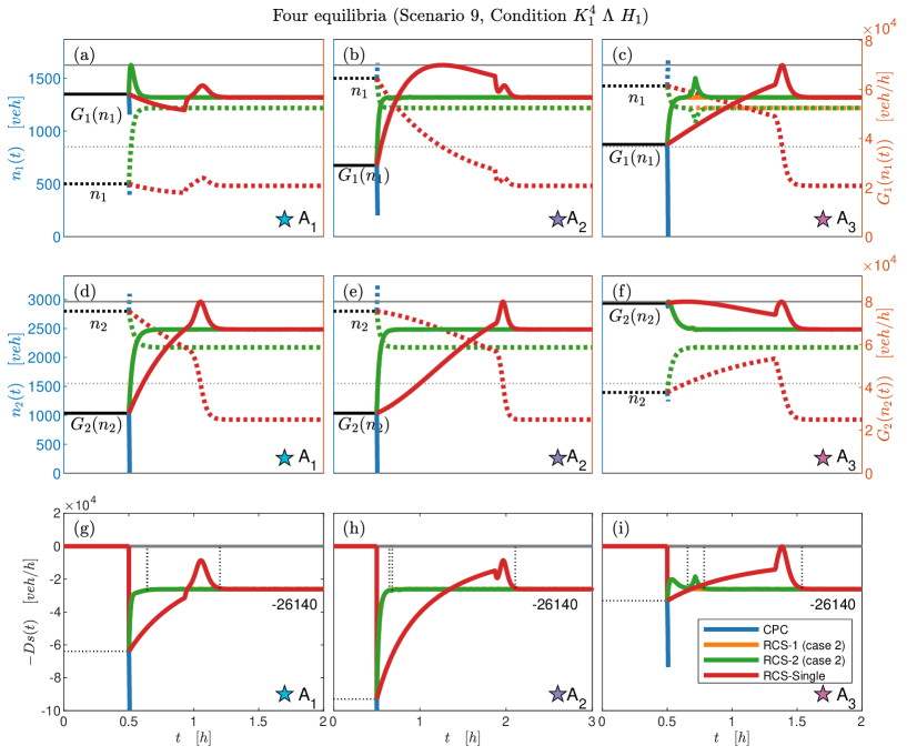
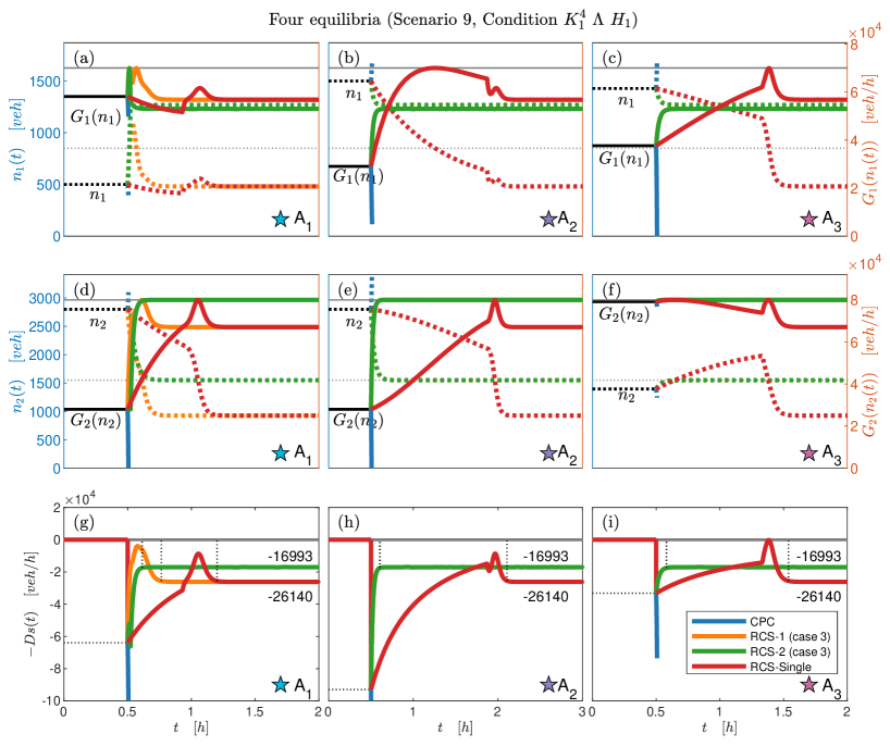
In this section, we compare our proposed control schemes (RCS-1 and RCS-2) with two classical perimeter control strategies (RCS-single in Gao et al. (2022) and CPC in Haddad and Geroliminis (2012)) to show the resilience of our approaches. We maintain the same MFD setup as in the previous section, and use scenario 9 as an example. Fig. 13(d) depicts the numerical simulation of phase portrait for the control system with RCS-single, where trajectories within the whole region recover to the original equilibrium . The key distinction between RCS-single and proposed schemes lies in the trajectories within the part: our proposed control schemes can recover to the alternative steady state , while RCS-single can only recover to the original equilibrium .
Then, we calculate the resilience measure (defined in Eq. (10)) under different control schemes. Resilience measures are situation-dependent, where situations referring to states (vehicle accumulations) after disturbances, also known as initial recovery states. For instance, we assume state perturbations suddenly occur at moment . Situation denotes the disturbed state at as (). Here, we consider three situations, i.e., , and , marked as three pentagrams in Fig. 13. Following these trajectories (the black lines in Fig. 13) departing from the pentagrams, we plot the vehicle accumulation , completion flow rate , and the numerical diagrams of deviation from maximum completion flow ( and ) evolving with time under each control scheme (CPC, RCS-1, RCS-2, RCS-single) in Fig. 15. Here we use Case 1 (corresponding to Fig. 13(b) and 13(c)) as an example to illustrate performance the proposed control schemes, and the results for Case 2 and Case 3 can be found in App. 8, Fig. 24 and Fig. 25.
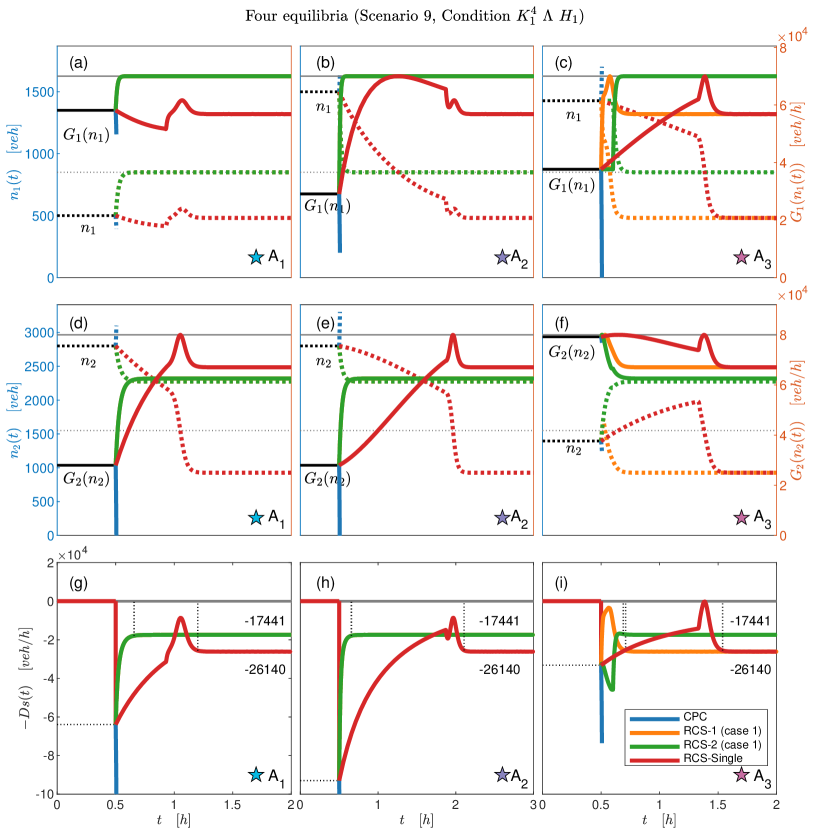
Clearly, as depicted in Fig. 15(g), (h), and (i), traffic system collapses rapidly under CPC (blue solid line) (within 0.006 for , 0.01 for and 0.007 for ); under RCS-single (red solid line), system initially rises slowly approaching maximum completion flow, then rebounds and stabilizes at a deviation of 26140 (within 0.70 for , 1.61 time for and 1.04 for ); under the proposed RCS-1 (yellow solid line), the system swiftly recovers to a deviation of 17441 (within 0.16 for and 0.16 for , coinciding with the green solid line), or it first rises rapidly approaching the maximum completion flow, then rebounds and stabilizes at a deviation of 26140 (within 0.21 for ); under the proposed RCS-2 (green solid line), the system swiftly recovers to a deviation of 17441 (within 0.16 for and 0.16 for ), or it resists the continued deterioration of the system, guiding a swift recovery, and stabilizes at a deviation of 17441 (within 0.19 for ). Here, we take as an example to elucidate the reasons for the aforementioned phenomena. Under CPC, the vehicle accumulation (Fig. 15(d), blue dotted line) develops from 2800 to a jam vehicle accumulation of 3100 within 0.006 , leading to the completion flow (blue solid line) tending towards 0. This causes Region 2 to enter a gridlock state from which it cannot recover. Under RCS-single, the vehicle accumulation (Fig. 15(a), red dotted line) initially decreases slowly from 500 , then slowly increases before decreasing again, finally stabilizing at the original equilibrium of 481 . Correspondingly, the completion flow decreases slowly, then increases slowly, before decreasing again and stabilizing at 56818 . Simultaneously, the vehicle accumulation (Fig. 15(d), red dotted line) decreases slowly at first, then rapidly decreases and stabilizes at 926 . Consequently, the completion flow (Fig. 15(d), red solid line) first rises slowly to maximum completion flow, then rapidly decreases and stabilizes at 67045 . Therefore, the recoverability of RCS-single is guaranteed, but with a longer duration. Under the proposed RCS-1 and RCS-2, due to high travel demand, the vehicle accumulation (Fig. 15(a), green dotted line) rapidly increases from 500 and stabilizes at 850, resulting in the completion flow (Fig. 15(a), green solid line) rapidly rising and stabilizing at the maximum completion flow of . Simultaneously, the vehicle accumulation (Fig. 15(b), green dotted line) rapidly decreases from 2800 to 2274 , leading the completion flow quickly stabilized at 62559 . Consequently, RCS-1 and RCS-2 can ensure rapid recoverability, outperforming RCS-single. It is noteworthy that in this scenario, RCS-1 and RCS-2 exhibit identical recovery trajectories. We also provide the cases of RCS-1 and RCS-2 employing different recovery trajectories, as shown in Fig. 15(c), (f), and (i).
For a more accurate comparison, based on Fig. 15 and Eq. (10), we integrate the curve of versus to obtain the value of resilience measure, under RCS-1, RCS-2, and RCS-single. The results are outlined in Table 2. Noteworthy, the absolute value of corresponds to the area of the resilience triangle during the recovery period, and it signifies the loss of actual completed trips compared to the maximum number of trips that could have been completed during the recovery period. A larger resilience measure corresponds to a smaller area of the resilience triangle (less loss), indicating greater resilience. As presented in Table 2, for all three Situations (, and ), resilience measures for RCS-1 and RCS-2 are significantly larger than RCS-single, demonstrating exceptional recovery capabilities.
| resilience control | |||||||||
|---|---|---|---|---|---|---|---|---|---|
| Case 1 | Case 2 | Case 3 | Case 1 | Case 2 | Case 3 | Case 1 | Case 2 | Case 3 | |
| RCS-1 | -4031 | -4384 | -3110 | -4284 | -5646 | -3681 | -4250 | -3302 | -1710 |
| RCS-2 | -4031 | -4384 | -5800 | -4284 | -6558 | -6615 | -3776 | -3302 | -1744 |
| RCS-single | -24568 | -56501 | -20584 | -24568 | -56501 | -20584 | -24568 | -56501 | -20584 |
6 Conclusion
In this paper, we define the ecological resilience of urban traffic, and further propose a resilience control methodology from the perspective of ecological resilience. Specifically, the ecological resilience of urban traffics is defined by the ability for a traffic system to resist uncertain perturbations by shifting to alternative states. The resilience control methodology comprises three aspects: portraying the recoverable scopes, designing alternative steady states, controlling system to shift to alternative steady states for adapting large disturbances. Among them, the recoverable scopes are portrayed by inner and outer estimations of attraction regions; the alternative steady states are set close to the optimal state and outside the recoverable scopes of the original equilibrium; the controller ensures the local stability of the alternative steady states, without changing the trajectories inside the recoverable scopes of the original equilibrium as much as possible. We implemented the proposed control framework in a two-region traffic network described by parabolic MFD dynamic, and designed proposed control schemes (RCS-1 and RCS-2). Comparisons with the classical urban traffic resilience control schemes (CPC and RCS-single, etc.) show that, proposed resilience control schemes (RCS-1 and RCS-2) has a better adaptability and generates a greater resilience measure. Noteworthy, RCS-1 differs with RCS-2 in control intensity, control formulation and control effect. Note that, for multi-region (more than two-region) MFD dynamics, our resilience control idea can still be applied. The difficulty in implementing the resilience control idea is that for N-dimensional system, the equilibrium point will be more complex, and the attraction region maybe more difficult to obtain. Moreover, the inner estimation of attraction region we can obtain may shrink and the outer estimation of attraction region may expand, potentially affecting the effectiveness of the regulation scheme.
There is still work to be done in the future. Given this paper considers mainly constant MFD dynamics, and it is worth to extend the methodology of this paper to more general time-varying MFD dynamics in the future. Moreover, a feasible resilience control is provided in this paper, and future work will be extended to find an optimal resilience control scheme.
This work was supported by the National Key RD Program of China (No.2022YFA1005103), the National Natural Science Foundation of China (12371452, 72225012, 72288101, 71822101, 12101030) and the Fundamental Research Funds for the Central Universities.
References
- Aboudolas and Geroliminis (2013) Aboudolas K, Geroliminis N, 2013 Perimeter and boundary flow control in multi-reservoir heterogeneous networks. Transportation Research Part B: Methodological 55:265–281.
- Aghamohammadi and Laval (2020) Aghamohammadi R, Laval JA, 2020 Dynamic traffic assignment using the macroscopic fundamental diagram: A review of vehicular and pedestrian flow models. Transportation Research Part B: Methodological 137:99–118.
- Ampountolas, Zheng, and Geroliminis (2017) Ampountolas K, Zheng N, Geroliminis N, 2017 Macroscopic modelling and robust control of bi-modal multi-region urban road networks. Transportation Research Part B: Methodological 104:616–637.
- Blanchini (1995) Blanchini F, 1995 Nonquadratic lyapunov functions for robust control. Automatica 31(3):451–461.
- Bruneau et al. (2003) Bruneau M, Chang SE, Eguchi RT, Lee GC, O’Rourke TD, Reinhorn AM, Shinozuka M, Tierney K, Wallace WA, Von Winterfeldt D, 2003 A framework to quantitatively assess and enhance the seismic resilience of communities. Earthquake spectra 19(4):733–752.
- Daganzo, Gayah, and Gonzales (2011) Daganzo CF, Gayah VV, Gonzales EJ, 2011 Macroscopic relations of urban traffic variables: Bifurcations, multivaluedness and instability. Transportation Research Part B: Methodological 45(1):278–288.
- Dakos and Kéfi (2022) Dakos V, Kéfi S, 2022 Ecological resilience: What to measure and how. Environmental Research Letters 17(4):043003.
- Dantsuji, Fukuda, and Zheng (2021) Dantsuji T, Fukuda D, Zheng N, 2021 Simulation-based joint optimization framework for congestion mitigation in multimodal urban network: a macroscopic approach. Transportation 48:673–697.
- Folke (2006) Folke C, 2006 Resilience: The emergence of a perspective for social ecological systems analyses. Global Environ Change 16(3):253–267.
- Folke et al. (2010) Folke C, Carpenter SR, Walker B, Scheffer M, Chapin T, Rockström J, 2010 Resilience thinking: integrating resilience, adaptability and transformability. Ecology and society 15(4).
- Gao et al. (2022) Gao S, Li D, Zheng N, Hu R, She Z, 2022 Resilient perimeter control for hyper-congested two-region networks with mfd dynamics. Transportation Research Part B: Methodological 156:50–75.
- Geroliminis and Daganzo (2008) Geroliminis N, Daganzo CF, 2008 Existence of urban-scale macroscopic fundamental diagrams: Some experimental findings. Transportation Research Part B: Methodological 42(9):759–770.
- Gunderson (2000) Gunderson LH, 2000 Ecological resilience–in theory and application. Annual review of ecology and systematics 425–439.
- Haddad (2015) Haddad J, 2015 Robust constrained control of uncertain macroscopic fundamental diagram networks. Transportation Research Part C 59(OCT.):323–339.
- Haddad and Geroliminis (2012) Haddad J, Geroliminis N, 2012 On the stability of traffic perimeter control in two-region urban cities. Transportation Research Part B: Methodological 46(9):1159–1176.
- Haddad and Mirkin (2020) Haddad J, Mirkin B, 2020 Resilient perimeter control of macroscopic fundamental diagram networks under cyberattacks. Transportation Research Part B: Methodological 132:44–59.
- Haddad and Zheng (2020) Haddad J, Zheng Z, 2020 Adaptive perimeter control for multi-region accumulation-based models with state delays. Transportation Research Part B: Methodological 137:133–153.
- Holling (1973) Holling CS, 1973 Resilience and stability of ecological systems. Annual review of ecology and systematics 1–23.
- Holling (1996) Holling CS, 1996 Engineering resilience versus ecological resilience. Engineering within ecological constraints 31(1996):32.
- Hosseini, Barker, and Ramirez-Marquez (2016a) Hosseini S, Barker K, Ramirez-Marquez JE, 2016a A review of definitions and measures of system resilience. Reliability Engineering & System Safety 145:47–61.
- Hosseini, Barker, and Ramirez-Marquez (2016b) Hosseini S, Barker K, Ramirez-Marquez JE, 2016b A review of definitions and measures of system resilience. Reliability Engineering & System Safety 145:47–61.
- Huang et al. (2020a) Huang HJ, Xia T, Tian Q, Liu TL, Wang C, Li D, 2020a Transportation issues in developing china’s urban agglomerations. Transport Policy 85:A1–A22.
- Huang et al. (2020b) Huang Y, Xiong J, Sumalee A, Zheng N, Lam W, He Z, Zhong R, 2020b A dynamic user equilibrium model for multi-region macroscopic fundamental diagram systems with time-varying delays. Transportation Research Part B: Methodological 131:1–25.
- Johari et al. (2021) Johari M, Keyvan-Ekbatani M, Leclercq L, Ngoduy D, Mahmassani HS, 2021 Macroscopic network-level traffic models: Bridging fifty years of development toward the next era. Transportation Research Part C: Emerging Technologies 131:103334.
- Khwais and Haddad (2022) Khwais M, Haddad J, 2022 Optimal presignal control for two-mode traffic at isolated signalized intersections. Transportation science 57(2):376–398.
- Kouvelas, Saeedmanesh, and Geroliminis (2023) Kouvelas A, Saeedmanesh M, Geroliminis N, 2023 A linear-parameter-varying formulation for model predictive perimeter control in multi-region mfd urban networks. Transportation Science 57(6):1496–1515.
- Laval, Leclercq, and Chiabaut (2017) Laval JA, Leclercq L, Chiabaut N, 2017 Minimal parameter formulations of the dynamic user equilibrium using macroscopic urban models: Freeway vs city streets revisited. Transportation research procedia 23:517–530.
- Li, Yildirimoglu, and Ramezani (2021) Li Y, Yildirimoglu M, Ramezani M, 2021 Robust perimeter control with cordon queues and heterogeneous transfer flows. Transportation Research Part C: Emerging Technologies 126:103043.
- Liao (2012) Liao KH, 2012 A theory on urban resilience to floods-a basis for alternative planning practices. Ecology and society 17(4).
- Mariotte, Leclercq, and Laval (2017) Mariotte G, Leclercq L, Laval JA, 2017 Macroscopic urban dynamics: Analytical and numerical comparisons of existing models. Transportation Research Part B: Methodological 101:245–267.
- Martin-Breen and Anderies (2011) Martin-Breen P, Anderies JM, 2011 Resilience: A literature review .
- Mohajerpoor, Cai, and Ramezani (2023) Mohajerpoor R, Cai C, Ramezani M, 2023 Optimal traffic signal control of isolated oversaturated intersections using predicted demand. IEEE Transactions on Intelligent Transportation Systems 24(1):815–826.
- O’Neill et al. (1986) O’Neill RV, Deangelis DL, Waide JB, Allen TF, Allen GE, 1986 A hierarchical concept of ecosystems (Princeton University Press).
- Pimm (1984) Pimm SL, 1984 The complexity and stability of ecosystems. Nature 307(5949):321–326.
- Ramezani, Haddad, and Geroliminis (2015) Ramezani M, Haddad J, Geroliminis N, 2015 Dynamics of heterogeneity in urban networks: aggregated traffic modeling and hierarchical control. Transportation Research Part B: Methodological 74:1–19.
- Ratschan and She (2010) Ratschan S, She Z, 2010 Providing a basin of attraction to a target region of polynomial systems by computation of lyapunov-like functions. SIAM Journal on Control and Optimization 48(7):4377–4394.
- Rölfer, Celliers, and Abson (2022) Rölfer L, Celliers L, Abson D, 2022 Resilience and coastal governance: knowledge and navigation between stability and transformation. Ecology and Society 27(2).
- Scheffer et al. (1993) Scheffer M, Hosper SH, Meijer ML, Moss B, Jeppesen E, 1993 Alternative equilibria in shallow lakes. Trends in ecology & evolution 8(8):275–279.
- Scoones et al. (2020) Scoones I, Stirling A, Abrol D, Atela J, Charli-Joseph L, Eakin H, Ely A, Olsson P, Pereira L, Priya R, et al., 2020 Transformations to sustainability: combining structural, systemic and enabling approaches. Current Opinion in Environmental Sustainability 42:65–75.
- She and Xue (2014) She Z, Xue B, 2014 Discovering multiple lyapunov functions for switched hybrid systems. SIAM Journal on Control and Optimization 52(5):3312–3340.
- She et al. (2020) She Z, Zhang A, Lu J, Hu R, Sam Ge S, 2020 Design proportional-integral-derivative/proportional-derivative controls for second-order time-varying switched nonlinear systems. International Journal of Robust and Nonlinear Control 30(5):1979–2000.
- Skafidas et al. (1999) Skafidas E, Evans RJ, Savkin AV, Petersen IR, 1999 Stability results for switched controller systems. Automatica 35(4):553–564.
- Su et al. (2020) Su Z, Chow AH, Zheng N, Huang Y, Liang E, Zhong R, 2020 Neuro-dynamic programming for optimal control of macroscopic fundamental diagram systems. Transportation Research Part C: Emerging Technologies 116:102628.
- Tilman and Downing (1994) Tilman D, Downing JA, 1994 Biodiversity and stability in grasslands. Nature 367(6461):363–365.
- Tsitsokas, Kouvelas, and Geroliminis (2023) Tsitsokas D, Kouvelas A, Geroliminis N, 2023 Two-layer adaptive signal control framework for large-scale dynamically-congested networks: Combining efficient max pressure with perimeter control. Transportation Research Part C: Emerging Technologies 152:104128.
- Walker et al. (2004) Walker B, Holling CS, Carpenter SR, Kinzig A, 2004 Resilience, adaptability and transformability in social–ecological systems. Ecology and society 9(2).
- Walker and Salt (2012) Walker B, Salt D, 2012 Resilience thinking: sustaining ecosystems and people in a changing world (Island press).
- Wang, She, and Ge (2020a) Wang S, She Z, Ge SS, 2020a Estimating minimal domains of attraction for uncertain nonlinear systems. IEEE Transactions on Systems, Man, and Cybernetics: Systems .
- Wang, She, and Ge (2020b) Wang S, She Z, Ge SS, 2020b Inner-estimating domains of attraction for nonpolynomial systems with polynomial differential inclusions. IEEE transactions on cybernetics .
- Wang et al. (2021) Wang S, Wu W, Lu J, She Z, 2021 Inner-approximating domains of attraction for discrete-time switched systems via multi-step multiple lyapunov-like functions. Nonlinear Analysis: Hybrid Systems 40:100993.
- Willems (1971) Willems JC, 1971 The generation of lyapunov functions for input-output stable systems. SIAM Journal on Control 9(1):105–134.
- Yang, Menendez, and Zheng (2019) Yang K, Menendez M, Zheng N, 2019 Heterogeneity aware urban traffic control in a connected vehicle environment: A joint framework for congestion pricing and perimeter control. Transportation Research Part C: Emerging Technologies 105:439–455.
- Yang, Zheng, and Menendez (2018) Yang K, Zheng N, Menendez M, 2018 Multi-scale perimeter control approach in a connected-vehicle environment. Transportation Research Part C: Emerging Technologies 94:32–49.
- Zeng et al. (2020) Zeng G, Gao J, Shekhtman L, Guo S, Lv W, Wu J, Liu H, Levy O, Li D, Gao Z, et al., 2020 Multiple metastable network states in urban traffic. Proceedings of the National Academy of Sciences 117(30):17528–17534.
- Zeng et al. (2019) Zeng G, Li D, Guo S, Gao L, Gao Z, Stanley HE, Havlin S, 2019 Switch between critical percolation modes in city traffic dynamics. Proceedings of the National Academy of Sciences 116(1):23–28.
- Zeng et al. (2022) Zeng X, Yu Y, Yang S, Lv Y, Sarker MNI, 2022 Urban resilience for urban sustainability: Concepts, dimensions, and perspectives. Sustainability 14.
- Zhang (2006) Zhang Z, 2006 Qualitative theory of differential equations, volume 101 (American Mathematical Soc.).
- Zheng et al. (2018) Zheng X, She Z, Liang Q, Li M, 2018 Inner approximations of domains of attraction for a class of switched systems by computing lyapunov-like functions. International Journal of Robust and Nonlinear Control 28(6):2191–2208.
- Zhong et al. (2020a) Zhong R, Cai H, Xu D, Chen C, Sumalee A, Pan T, 2020a Dynamic feedback control of day-to-day traffic disequilibrium process. Transportation Research Part C: Emerging Technologies 114:297–321.
- Zhong et al. (2018a) Zhong R, Chen C, Huang Y, Sumalee A, Lam W, Xu D, 2018a Robust perimeter control for two urban regions with macroscopic fundamental diagrams: A control-lyapunov function approach. Transportation Research Part B: Methodological 117:687–707.
- Zhong et al. (2018b) Zhong R, Huang Y, Chen C, Lam W, Xu D, Sumalee A, 2018b Boundary conditions and behavior of the macroscopic fundamental diagram based network traffic dynamics: A control systems perspective. Transportation Research Part B: Methodological 111:327–355.
- Zhong et al. (2020b) Zhong R, Xie X, Luo J, Pan T, Lam W, Sumalee A, 2020b Modeling double time-scale travel time processes with application to assessing the resilience of transportation systems. Transportation research part B: methodological 132:228–248.
7 Global phase portrait and attraction region for four-equilibria system
we will consider the four-equilibria cases, derive its qualitative characteristics under CPC ( and ), and further provide an inner and outer estimations of attraction regions. Specifically, local stability verification of the four-equilibria system will be shown in App. 7.1; global phase portrait derivation is performed in App. 7.2; and spontaneous attraction region estimation of four-equilibria system will be included in App. 7.3.
7.1 Local stability verification
According to Condition , we have:
| (22) |
We first verify the local stability of the four equilibria for system (1) satisfying (22). Under Condition (), we have the following proposition for its four equilibria.
Proposition 7.1
Under Condition (), for system (1), is a locally stable node, and are saddle points, is an unstable node.
Proof: For system (1), we can get the derivative operator () at the equilibrium as follows:
Thus, the two eigenvalues () of satisfy:
| (23) |
Note that the discriminant for Eq. (23) is:
-
1.
For =(,), we can get , then Eq. (23) has two real roots and . Moreover, we have: , , which implies . Thus, we can conclude the equilibrium point is a locally stable node.
-
2.
For =(,), we can get , then Eq. (23) has two real roots and , where . Moreover, we have: , which implies . Thus, we have that the equilibrium point is a saddle point.
-
3.
For =(,), we also have , then Eq. (23) has two real roots and , where . Moreover, we have: , which indicates . Thus, is a saddle point.
-
4.
For =(,), we have , Moreover, the two real roots and of Eq. (23) satisfy , , which implies . Thus, is an unstable node.
7.2 Global phase portrait derivation
Subsequently, for the four-equilibria system (1) under Condition (), the global phase portrait will be derived. First letting and , we simplify system (1) as:
| (24) |
where , , , and . Obviously, the corresponding four equilibria of system (24) are , , and . Note that the four equilibria of the original system (1) are , , , and . Moreover, since and , we have that Condition (or inequality (22)) holds if and only if Condition ():
| (25) |
holds. Further, Condition () can be divided into five sub-conditions:
-
(1)
Condition : ;
-
(2)
Condition :
-
(3)
Condition :
-
(4)
Condition : ;
-
(5)
Condition :
Thus in the following, we will discuss the global qualitative characteristics and attraction region for equivalence system (24) under Condition () respectively, where .
To begin with, we consider the phase portrait under Condition (), which can be partitioned into four sub-Conditions: (), (), () and ().
First consider Condition (). Following the steps in Sec. 3.2, we have that: the demarcation lines are and , portrayed as the red and blue dotted curve respectively in Fig. 16(a). In addition, we have and on these two red curves, indicating when or holds and when holds. Similarly, we have and on these two blue curves, implying when or holds and when holds. Obviously, we can obtain nine unbounded regions in divided by these four curves. Moreover, Table 3 summarizes the symbols of () in these nine regions. On the basis of Table 3, the phase portrait of (24) under Condition () can be obtained, as shown in Fig. 16(a). Subsequently, based on the phase portrait 5(a), by utilizing proof by contradiction, we can verify that regions B, G and F are positive invariant sets. Since the trajectories starting from B, G and F will not escape, there exist no close orbits for system (24) under Condition ().
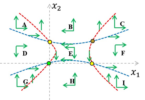
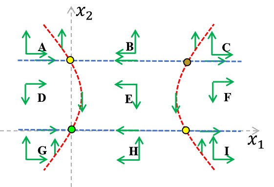
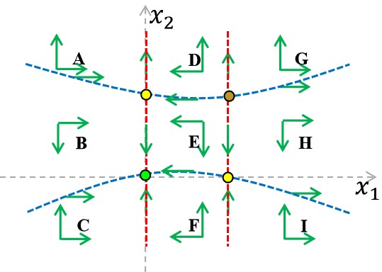
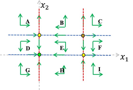
| Derivative | Symbol in the region | ||||||||
| A | B | C | D | E | F | G | H | I | |
Then, for Conditions (), () and (), we can also simplify the system (24) and then perform the above analysis. In a similar way, we can obtain four corresponding curves under each Condition, which separate to nine unbounded regions. Then the corresponding phase portraits of (24) under these three Conditions can be acquired, as shown in Figs. 16(b), 16(c) and 16(d). Further, we can also obtain the positive invariant sets under each Condition, which verify that there is no close orbit for system (24) under Conditions (), () and (). Thus, there exists no close orbit, for the system (1) under Condition .
7.3 Spontaneous attraction region estimation
Based on the nonexistence of close orbits and Fig. 16, we will next analyze the attraction region of the locally stable node . For this purpose, we wish to find certain corresponding separatrices of system (24) under Conditions (), (), () and (). However, due to the increased number of equilibria, it seems very difficult to find certain separatrices directly. Thus, we will first find inner and outer estimations of attraction regions, and then find certain corresponding separatrices under the above four conditions.
To start with, we consider Condition (). The two red dotted demarcation lines can be denoted as (), where . Similarly, the two blue dotted demarcation lines can be denoted as (), where . Obviously, the vertex of the line is and the vertex of the line () is . Subsequently, in light of Fig. 16(a), we can similarly verify that the region (the light yellow region shown in Fig. 17(a)) is a positive invariant set, where with
Moreover, by similar analysis to in two-equilibria case, we can arrive that , i.e., is an outer estimation of attraction region for .
In addition, (the light blue region shown in Fig. 17(a)) is also a positive invariant set, where
with
Further, we can prove that is an inner estimation of attraction region for by following two steps. Firstly, the trajectory starting from any point in will entering the bounded region as , where
as we have on the left boundary of and on the lower boundary of . Secondly, the trajectory starting from any point in bounded region will go to as , since there is no closed orbit, and there exists only one stable node in the bounded region (Zhang (2006)).
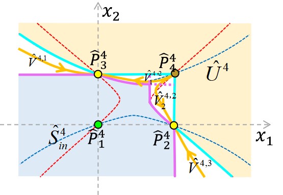
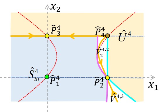
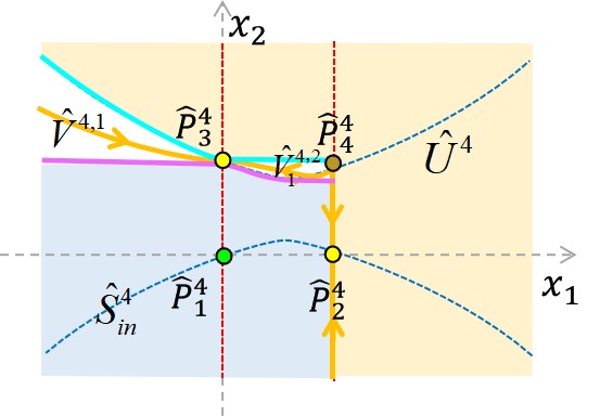
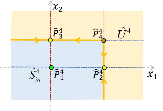
As for Conditions (), () and (), through similar analysis, we can obtain the inner and outer estimations of attraction regions for , as shown in the Figs. 17(b), 17(c) and 17(d). Further, letting and , the inner and outer estimations of attraction regions for can be obtained. Denoting and , where and , we can arrive at the following theorem.
Theorem 7.2
Under Condition (), for the local stable point , we have , where the inner estimation of attraction region and the outer estimation of attraction region are defined as follows:
-
(1)
Under Condition (),
-
(2)
Under Condition (),
-
(3)
Under Condition (),
-
(4)
Under Condition (),
Note that () holds all the time.
Clearly, according to Theorem 7.2, the inner and outer estimations of attraction regions for under () with can be obtained, as shown in the Figs. 9(a)–9(d).
Moreover, we will derive the boundaries of the attraction region of under Condition (), by finding certain corresponding separatrices located in of equivalent systems (24), as shown in Fig. 17(a), where
and , where
Obviously, we can obtain a stable separatrix for the saddle point and a stable separatrix for the saddle point . Moreover, we can further obtain another stable separatrix of , which satisfy and , by following two steps. Firstly, we can verify that the region is a negative invariant set, otherwise there will exist contradiction with the trajectory direction at the boundary line of region . Secondly, the trajectory starting from any point in bounded region will go to as , since there is no closed orbit, and there exists only one unstable node in the bounded region (Zhang (2006)). Similarly, we can obtain another stable separatrix for , which satisfies and . Clearly, these four separatrices are exactly the boundaries of the attraction region for .
Further, letting and , the attraction region boundary for under Condition () can be obtained. Denoting () to be the two stable separatrices of , and () to be the two stable separatrices of , the below theorem can be arrived.
Theorem 7.3
Under Condition (), for the local stable point , we have , where
satisfying , and are defined as:
and
with and . Note that () holds all the time.
In summary, the attraction region of under corresponding conditions are plotted as light pink zones in the Figs. 9(a)-9(d).
Secondly, we consider Condition (), which can be partitioned into two sub-Conditions: () and (). Note that and . By repeating the analysis as above, the corresponding phase portraits of (24) under these two sub-conditions can be obtained; and further prove that there is no close orbit for system (24) under above two sub-conditions. In addition, we can obtain the inner and outer estimations of attraction regions for , and deduce the boundary of attraction region for , as shown in the Figs. 18(a) and 18(b). Further, letting and , we can obtain the inner and outer estimations of attraction regions for which are defined in Theorem 7.2 (1), and the attraction region boundary for under Conditions () and (), as shown in Figs. 9(e) and 9(f).
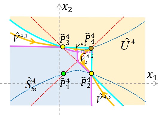
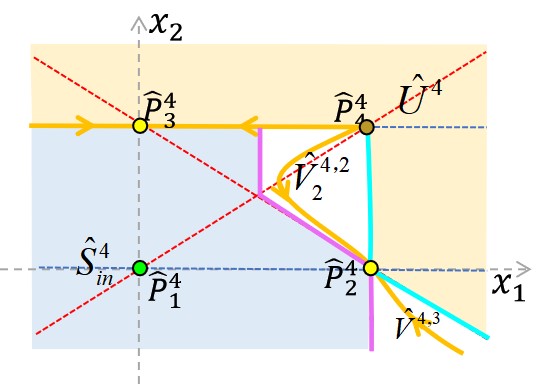
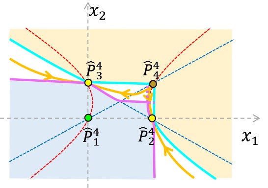
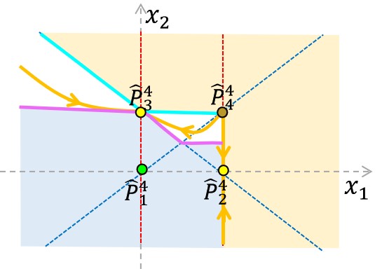
Thirdly, we analyze the phase portrait and the attraction region of under Condition (), which can be partitioned into two sub-Conditions: () and (). Note that and . Notice that Condition () is symmetric to Condition (), so the analysis process and results are similar. Thus, we can obtain the inner and outer estimations of attraction regions for in a similar way, as shown in Figs. 18(c) and 18(d). Further, letting and , the attraction region of under Conditions () and () can be obtained, as shown in Figs. 9(g) and 9(h).
Fourthly, we consider Condition (), which can be partitioned into two sub-Conditions: Condition () and (). Note that and .
We first consider Condition (). For system (24) under Condition (), following the steps as Condition (), the global phase portrait can be obtained, as shown in Fig. 19(a); further prove that there exist no close orbits; and subsequently derive the inner estimation of attraction region and the outer estimation of attraction region , where
and
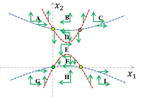
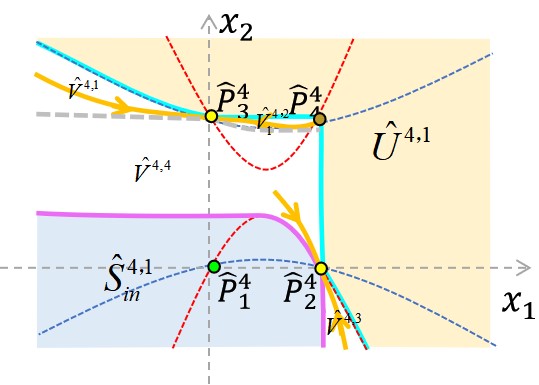
Thus, we will next deduce the boundaries of the attraction region of by finding certain corresponding separatrices located in of equivalent systems (24), as shown in Fig. 19(b), where and . By similar analysis as above, we can obtain a stable separatrix for the saddle point ; a stable separatrix for the saddle point ; and another stable separatrix of , which satisfy and . Note that and are defined above. As for another stable separatrix for in , there are three types, where in type 1, ; in type 2, ; and in type 3, ; as shown in Figs. 20(a), 20(b) and 20(c), respectively.
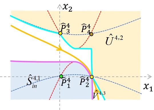
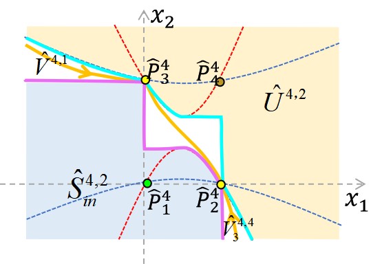
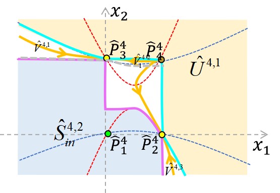
Further, we can refine the inner and outer estimations of attraction regions under each type. Specifically, In type 1, the outer estimation of attraction region can be refined as , where
since the region is a negative invariant set and the trajectory starting from any point in bounded region will go to as . In type 2, the outer estimation of attraction region can also be refined as for the same reason. Moreover, the inner estimation of attraction region can be refined as , where
since any trajectory starting from the region will also go to as . In type 3, the inner estimation of attraction region can be refined as for the same reason.
In summary, the refined inner and outer estimations of attraction regions in each type are obtained, as shown in Figs. 20(a), 20(b) and 20(c). Then, letting and , we can obtain the attraction region, inner and outer estimations of attraction regions in each type of system (1) under Conditions (), which are shown in Fig. 20. Moreover, denoting and , where , the below theorem can be arrived.
Theorem 7.4
Under Condition (), for the local stable point , we have , where , the inner estimation of attraction region and outer estimation of attraction region have three types, which are defined as follows:
-
(1)
In type 1: , where represents when and when ;
-
(2)
In type 2: , where represents when , represents when , and represents when ;
-
(3)
In type 3: is defined in Theorem 7.3;
Note that () holds all the time.
Then, for Conditions (), we can also simplify the system (24) and then perform the above analysis. In a similar way, we can obtain the phase portrait for system (24) and further verify that there are no close orbits under Conditions (). Thus, we can obtain three types of attraction regions, and further obtain three types of refined the inner and outer estimations of attraction regions under each type, as shown in Figs. 21(a), 21(b) and 21(c). Then letting and , we can obtain three types of attraction regions of (1) under Conditions (), as shown in Figs. 9(j), 9(n) and 9(r).
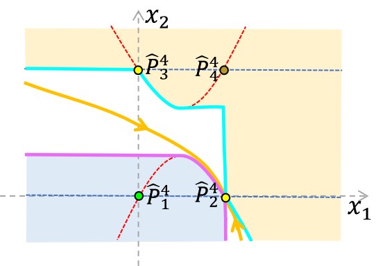
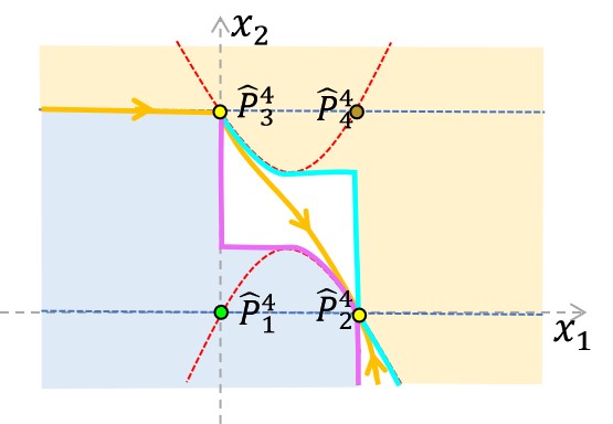
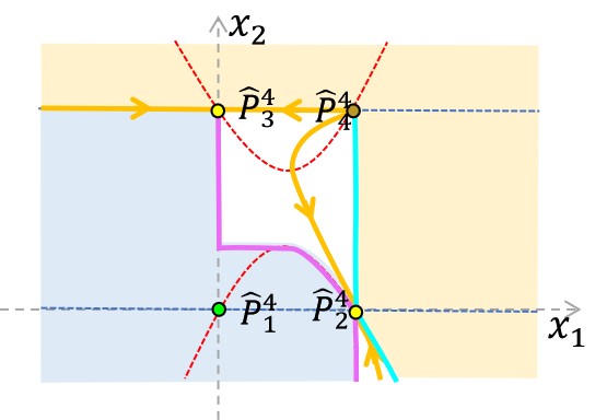


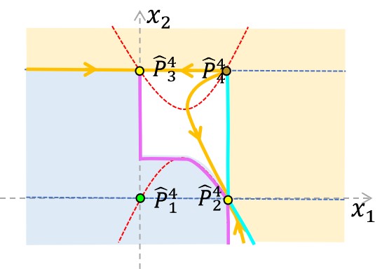
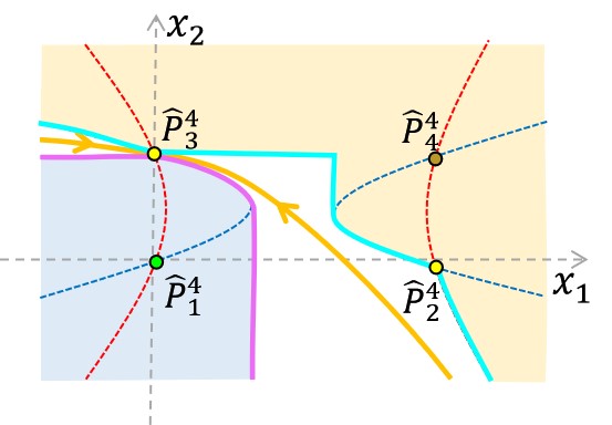
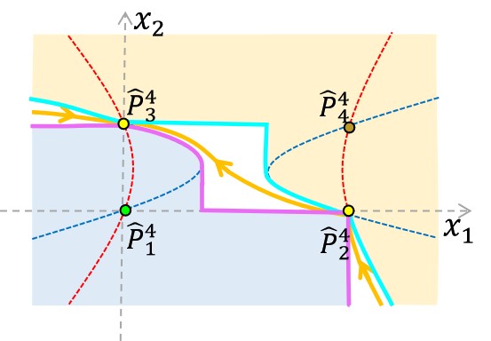
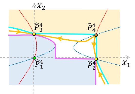
Finally, we analyze the phase portrait and the attraction region of under Condition (), which can be partitioned into two sub-Conditions: () and (). Note that and . Notice that Condition () is symmetric to Condition (), so the analysis process and results are similar. By repeating the analysis as above, we can get the refined results under Conditions () and (), as shown in Figs. 21 and 9.
8 Numerical verification of the Global phase portrait and attraction region
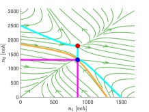
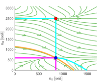
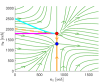
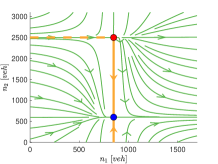
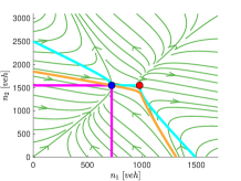
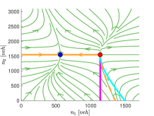
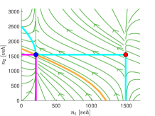
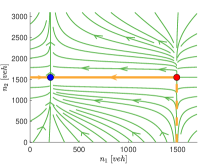
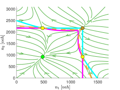

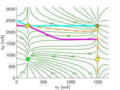
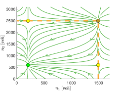
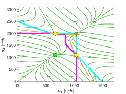
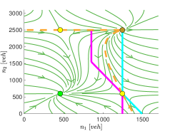
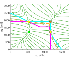
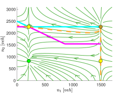
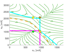
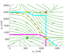
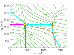
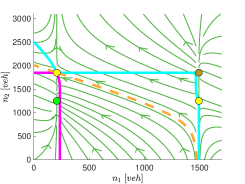
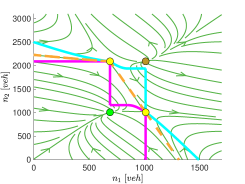
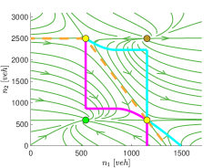
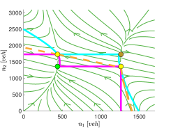
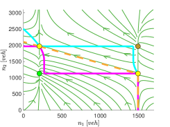
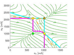
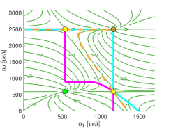
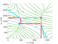
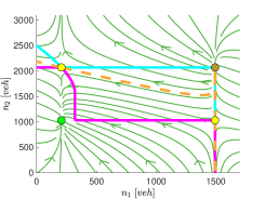
| Scenarios | Flow rates | Network-outside demands | Satisfying Condition | Corresponding phase portrait | ||
|---|---|---|---|---|---|---|
| Scenario 1 | Condition | Fig. 22(a) | ||||
| Scenario 2 | Condition | Fig. 22(b) | ||||
| Scenario 3 | Condition | Fig. 22(c) | ||||
| Scenario 4 | Condition | Fig. 22(d) | ||||
| Scenario 5 | Condition | Fig. 22(e) | ||||
| Scenario 6 | Condition | Fig. 22(f) | ||||
| Scenario 7 | Condition | Fig. 22(g) | ||||
| Scenario 8 | Condition | Fig. 22(h) | ||||
| Scenario 9 | Condition | Fig. 23(a) | ||||
| Scenario 10 | Condition | Fig. 23(b) | ||||
| Scenario 11 | Condition | Fig. 23(c) | ||||
| Scenario 12 | Condition | Fig. 23(d) | ||||
| Scenario 13 | Condition | Fig. 23(e) | ||||
| Scenario 14 | Condition | Fig. 23(f) | ||||
| Scenario 15 | Condition | Fig. 23(g) | ||||
| Scenario 16 | Condition | Fig. 23(h) | ||||
| Scenario 17 | Condition | Fig. 23(i) | ||||
| Scenario 18 | Condition | Fig. 23(m) | ||||
| Scenario 19 | Condition | Fig. 23(q) | ||||
| Scenario 20 | Condition | Fig. 23(j) | ||||
| Scenario 21 | Condition | Fig. 23(n) | ||||
| Scenario 22 | Condition | Fig. 23(r) | ||||
| Scenario 23 | Condition | Fig. 23(k) | ||||
| Scenario 24 | Condition | Fig. 23(o) | ||||
| Scenario 25 | Condition | Fig. 23(s) | ||||
| Scenario 26 | Condition | Fig. 23(l) | ||||
| Scenario 27 | Condition | Fig. 23(p) | ||||
| Scenario 28 | Condition | Fig. 23(t) | ||||