Characterisation of the TOI-421 planetary system using CHEOPS, TESS, and archival radial velocity data

Abstract

Context. The TOI-421 planetary system contains two sub-Neptune-type planets ($P_{\rm b}\sim 5.2$ days, $T_{\rm eq,b}\sim 900$ K, and $P_{\rm c}\sim 16.1$ days, $T_{\rm eq,c}\sim 650$ K) and is a prime target to study the formation and evolution of planets and their atmospheres. The inner planet is especially interesting as the existence of a hydrogen-dominated atmosphere at its orbital separation cannot be explained by current formation models without previous orbital migration.

Aims. We aim to improve the system parameters to further use them to model the interior structure and simulate the atmospheric evolution of both planets, to finally gain insights into their formation and evolution. We also investigate the possibility of detecting transit timing variations (TTVs).

Methods. We jointly analysed photometric data of three TESS sectors and six CHEOPS visits as well as 156 radial velocity data points to retrieve improved planetary parameters. We also searched for TTVs and modelled the interior structure of the planets. Finally, we simulated the evolution of the primordial H-He atmospheres of the planets using two different modelling frameworks.

Results. We determine the planetary radii and masses of TOI-421 b and c to be $R_{\rm b}=2.64\pm 0.08\,R_{\oplus}$, $M_{\rm b}=6.7\pm 0.6\,M_{\oplus}$, $R_{\rm c}=5.09\pm 0.07\,R_{\oplus}$, and $M_{\rm c}=14.1\pm 1.4\,M_{\oplus}$. Using these results we retrieved average planetary densities of $\rho_{\rm b}=0.37\pm 0.05\,\rho_{\oplus}$ and $\rho_{\rm c}=0.107\pm 0.012\,\rho_{\oplus}$. We do not detect any statistically significant TTV signals. Assuming the presence of a hydrogen-dominated atmosphere, the interior structure modelling results in both planets having extensive envelopes. While the modelling of the atmospheric evolution predicts for TOI-421 b to have lost any primordial atmosphere that it could have accreted at its current orbital position, TOI-421 c could have started out with an initial atmospheric mass fraction somewhere between $10$ and $35\%$.

Conclusions. We conclude that the low observed mean density of TOI-421 b can only be explained by either a bias in the measured planetary parameters (e.g. driven by high-altitude clouds) and/or in the context of orbital migration. We also find that the results of atmospheric evolution models are strongly dependent on the employed planetary structure model.

1 Introduction

The exact mechanisms of planet formation and evolution are still highly debated. For example, the classical core-accretion model (e.g. Bodenheimer & Pollack 1986; Pollack et al. 1996) has been challenged by more recent theories predicting much faster planet formation, such as the pebble accretion model (Johansen & Lacerda 2010; Ormel & Klahr 2010; Lambrechts & Johansen 2012; Johansen et al. 2015). A large sample of diverse planets with a mass and radius measured at at least $3\sigma$ significance is needed to test and compare different formation and evolution models. Efforts to compile such a sample have recently been led by the Transiting Exoplanet Survey Satellite (TESS; Ricker et al. 2014) and the CHaracterising ExOPlanet Satellite (CHEOPS; Benz et al. 2021), in close collaboration with large ground-based observing campaigns conducted with high-resolution spectrographs such as the High Accuracy Radial velocity Planet Searcher (HARPS; Mayor et al. 2003), its twin HARPS-N (Cosentino et al. 2012), the Calar Alto high-Resolution search for M dwarfs with Exoearths with Near-infrared and optical Echelle Spectrographs (CARMENS; Quirrenbach et al. 2014), and the Echelle SPectrograph for Rocky Exoplanet and Stable Spectroscopic Observations (ESPRESSO; Pepe et al. 2021). More than 5500 exoplanets have been confirmed so far and over 950 of them have both radii and masses measured at more than 3$\sigma$ confidence.

To test different formation models, we must also understand how planets evolve. Processes such as atmospheric mass loss and orbital migration can have a significant impact on planet parameters such as mass and radius over the course of the evolution. Multi-planet systems are especially important in the context of constraining planet formation and evolution as they allow us to compare planets with different sizes and compositions in the same system, thus they are illuminated by the same star. The prime targets for investigating the evolution of primordial planetary atmospheres are planets that have retained some part of their initial hydrogen-dominated envelope accreted during their formation, while also having been subject to strong mass loss driven by internal thermal energy and/or absorption of high-energy – X-ray and extreme ultraviolet (EUV; together XUV) – stellar radiation. The almost 11 Gyrs old system hosting two sub-Neptune-like planets TOI-421 (Carleo et al. 2020) checks all of this criteria and therefore has become a gold-standard target to study planetary atmospheric evolution and its implications for planet formation scenarios.

Carleo et al. (2020) presented a first simulation of the atmospheric evolution using the tool presented by Kubyshkina et al. (2019a, b) and assuming a hydrogen-dominated atmosphere and a formation of the planets at the orbital separation at which they are currently observed. The tool simultaneously constrains the initial atmospheric mass fraction and the evolution of the stellar rotation rate, where the latter acts as a proxy for the XUV stellar emission. They find that their models provide no additional constraint on the stellar rotation history of TOI-421 upon that retrieved from observations of young open cluster stars. For planet c, they find an initial atmospheric mass fraction of roughly 30% and a present-day atmospheric mass fraction of roughly 10%, meaning the planet would have lost about two-thirds of its primordial atmosphere over the course of its evolution due to the absorption of XUV radiation. Instead, for TOI-421 b they find that the existence of a planet as observed by Carleo et al. (2020) is not possible within the framework of the employed model. Given the measured planetary parameters, the planet should have completely lost any hydrogen-dominated atmosphere within the first gigayear, independent of the rotational evolution of the host star. According to their simulations, the planet would either have to orbit about twice as far out than measured or could not host a hydrogen-dominated atmosphere.

TOI-421 b is not the first planet for which a discrepancy is observed between the low measured bulk density, compatible with the presence of a hydrogen-dominated atmosphere, and the predicted mass loss rates, which are too large to enable the presence of a low-density envelope. Lammer et al. (2016) find the same problem for CoRoT-24b and Cubillos et al. (2017) find that about 15% of mini-Neptunes out of a large sample detected mostly by the Kepler satellite also share this peculiar property. Carleo et al. (2020) already mention a few possible solutions to this problem. Most importantly, the considered atmospheric evolution framework assumes that planets form within the protoplanetary nebula at the observed orbital separation. A formation further out and a subsequent orbital migration to the present-day orbit would allow for both more hydrogen gas being accreted during the time before the dispersal of the nebula and possibly lower XUV fluxes during the earlier stages of planet evolution (particularly in the case of post-disk migration). Another possible explanation is the presence of high-altitude aerosols, which could lead to an overestimate of the planetary radius (Lammer et al. 2016; Cubillos et al. 2017; Gao & Zhang 2020). This possibility finds some support in both observations (e.g. Libby-Roberts et al. 2020; Chachan et al. 2020) and modelling (e.g. Wang & Dai 2019; Ohno & Tanaka 2021). There might also be a replenishment of light gases released from the crust into the atmosphere, which would in turn counteract the effect of escape (e.g. Kite et al. 2019). Finally, they also mention the possibility that there are biases in the observed planetary parameters; for example, undetected planets in the system might affect the mass measurements.

Kubyshkina et al. (2022a, b) use the planet parameters derived by Carleo et al. (2020) to model the atmospheric evolution of the planets using more sophisticated models. Kubyshkina et al. (2022a) first show that the effects of stellar wind on the overall mass loss of the planets are negligible, justifying the use of evolutionary models that do not account for stellar winds. Kubyshkina et al. (2022b) then expand the atmospheric evolution framework already employed in Carleo et al. (2020) by additionally accounting for planetary internal thermal evolution. They find similar results as Carleo et al. (2020): while within their model planet c has started out with an initial atmospheric mass fraction of $0.30\pm 0.07$, planet b would have had to start out with a very significant initial atmospheric mass fraction lying somewhere between $0.48$ and $0.71$. However, as mentioned before in Carleo et al. (2020), Kubyshkina et al. (2022b) also conclude that such a high initial atmospheric mass fraction is unlikely for such a planet. Using a model by Mordasini (2020) to estimate the amount of hydrogen a planetary core could accrete before the dispersal of the protoplanetary nebula as a function of mass and orbital separation, they find that planet b could not have formed with such an extensive initial envelope within the ice line, implying a formation scenario beyond the ice line. Lopez (2017) show that in the case of a formation beyond the ice line, the presence of water vapour in the atmosphere could significantly reduce the heating efficiency and thus the mass loss rates. This would also be consistent with most formation models, which predict sub-Neptunes to be water-rich (Alibert et al. 2013; Raymond et al. 2018; Venturini et al. 2020; Izidoro et al. 2021; Emsenhuber et al. 2021).

Finally, it must also be noted that none of the current atmospheric evolution models have taken the effects of the possible presence of a planetary magnetic field into account. The consequence of the presence of a planetary magnetic field for atmospheric mass loss is not trivial. It is believed that the escape is reduced by the confinement of ionised atmospheric species within the closed magnetic field lines, while it is enhanced by the escape of atmospheric ions through the polar regions of the open magnetic lines and re-connection on the night-side (Khodachenko et al. 2015; Sakai et al. 2018; Carolan et al. 2021).

In this work, we present new space-based photometric data of both planets obtained by CHEOPS and TESS and include them in a global analysis of both photometric and radial velocity datasets. By the addition of data obtained by a second, independent photometric instrument, the high precision photometric measurements obtained by CHEOPS, and the additional transits observed by TESS, we aim to decrease the uncertainties on the system parameters. We investigate the possibility of detecting TTVs. We model the interior structures of the planets within an Bayesian framework and use the updated planetary parameters to constrain different kinds of atmospheric evolution models that assume that both planets host a hydrogen-dominated atmosphere. We compare the performance and results of the different methods to both highlight their advantages and disadvantages as well as better understand the possible past evolution of TOI-421 b, a sub-Neptune in an orbit that would imply catastrophic hydrodynamic escape of any kind of primordial hydrogen-dominated atmosphere.

2 Stellar characterisation

The spectroscopic stellar parameters ($T_{\mathrm{eff}}$, $\log g$, microturbulence velocity, [Fe/H]) were estimated using the ARES+MOOG methodology, which is described in detail in Sousa et al. (2021); Sousa (2014); Santos et al. (2013). This was done by using the latest version of ARES (Sousa et al. 2007, 2015) to consistently measure the equivalent widths (EW) of selected iron lines on the combined HARPS spectrum of TOI-421. We used the list of iron lines presented in Sousa et al. (2008). A minimisation process is then used in this analysis to find the ionisation and excitation equilibrium to finally obtain the atmospheric parameters $T_{\mathrm{eff}}$, $\log g$, and microturbulence velocity. This process makes use of a grid of Kurucz model atmospheres (Kurucz 1993) and the radiative transfer code MOOG (Sneden 1973). We also derived a more accurate trigonometric surface gravity using recent GAIA data following the same procedure as described in Sousa et al. (2021), which provided a consistent value when compared with the spectroscopic surface gravity.

Using the aforementioned stellar atmospheric parameters, we determined the abundances of Na, Mg, Si, Ti, and Ni following the classical curve-of-growth analysis method described in Adibekyan et al. (2012, 2015). Similar to the stellar parameter determination, we used ARES to measure the EWs of the spectral lines of these elements, and again used a grid of Kurucz model atmospheres along with the radiative transfer code MOOG to convert the EWs into abundances, assuming local thermodynamic equilibrium. Abundances of the elements are presented in Table 1.

Using the results of our spectral analysis as priors, we built spectral energy distributions (SEDs) using stellar atmospheric models from two catalogues (Kurucz 1993; Castelli & Kurucz 2003) to compute the stellar radius of TOI-421 via a MCMC modified infrared flux method (IRFM; Blackwell & Shallis 1977; Schanche et al. 2020). From these SEDs, we compared synthetic and observed broadband photometry in the Gaia $G$, $G_{\mathrm{BP}}$, and $G_{\mathrm{RP}}$, 2MASS $J$, $H$, and $K$, and WISE $W1$ and $W2$ (Skrutskie et al. 2006; Wright et al. 2010; Gaia Collaboration et al. 2023) bandpasses to derive the stellar bolometric flux that is converted into effective temperature and angular diameter via the Stefan-Boltzmann law. Thus, we obtain the stellar radius by combining the angular diameter with the offset-corrected Gaia parallax (Lindegren et al. 2021). As our SEDs were constructed using two catalogues, we account for model uncertainties using a Bayesian modelling averaging of the radius posterior distributions and report a weighted average in Table 1.

The stellar effective temperature $T_{\mathrm{eff}}$, metallicity [Fe/H], and radius $R_{\star}$ along with their uncertainties constitute the basic input set for deriving both the stellar mass $M_{\star}$ and age $t_{\star}$ from stellar evolutionary models. To get a first pair of mass and age estimates, we applied the isochrone placement algorithm (Bonfanti et al. 2015, 2016), which interpolates the input parameters within pre-computed grids of PARSEC v1.2S (Marigo et al. 2017) isochrones and tracks. In addition to the basic input set, we further use $v\sin{i}=1.8\pm 1.0$ km s^-1 (Carleo et al. 2020) as input to let the isochrone fitting work in synergy with gyrochronology as detailed in Bonfanti et al. (2016) to better constrain mass and age. Additionally, a second pair of mass and age values was obtained with the Code Liègeois d’Évolution Stellaire (CLES; Scuflaire et al. 2008), which builds the evolutionary track best fitting the stellar input parameters following a Levenberg-Marquadt minimisation scheme (Salmon et al. 2021). After checking the mutual consistency of the two respective pairs of mass and age values via the $\chi^{2}$-based criterion outlined in Bonfanti et al. (2021a), we finally merged the results and obtained $M_{\star}=0.833_{-0.054}^{+0.048}\,M_{\odot}$ and $t_{\star}=10.9_{-5.2}^{+2.9}$ Gyr. See Bonfanti et al. (2021a) for further details about the specific statistical treatment.

Table 1: Adopted stellar parameters of TOI-421

Parameter	Value	Unit	Source
Gmag	$9.78$	-	SWEET-Cat
Spectral Type	G9V	-	C2020
$T_{\mathrm{eff}}$	$5291\pm 64$	K	This work
$\log g$	$4.48\pm 0.03$	-	This work
Radius	$0.866\pm 0.006$	$R_{\odot}$	This work
Mass	$0.833^{+0.048}_{-0.054}$	$M_{\odot}$	This work
Density	$1.29\pm 0.15$	$\rho_{\odot}$	This work
Age	$10.9_{-5.2}^{+2.9}$	Gyr	This work
Rotation Period	$39.6\pm 1.6$	days	This work
$\left[\mathrm{Fe/H}\right]$	$-0.044\pm 0.04$	-	This work
$\left[\mathrm{Ni/H}\right]$	$-0.04\pm 0.03$	-	This work
$\left[\mathrm{Mg/H}\right]$	$0.02\pm 0.04$	-	This work
$\left[\mathrm{Si/H}\right]$	$-0.05\pm 0.05$	-	This work
$\left[\mathrm{Ti/H}\right]$	$0.04\pm 0.06$	-	This work
$\left[\mathrm{Na/H}\right]$	$-0.05\pm 0.04$	-	This work
$v\sin{i}$	$1.8\pm 1.0$	km s-1	C2020

Table 2: Log of CHEOPS observations.

Visit	Start Date	End Date	Duration	Efficiency	File Key
No.	[UTC]	[UTC]	[hours]	[%]	-
			Planet b
1	2021-11-19 01:13	2021-11-19 13:18	12.09	66.0	CH_PR100024_TG013601_V0300
2	2021-12-10 03:32	2021-12-10 10:00	6.47	90.2	CH_PR100024_TG014701_V0300
3	2022-01-10 08:00	2022-01-10 15:05	7.09	67.6	CH_PR100024_TG014702_V0300
4	2022-11-28 14:27	2022-11-29 00:10	9.72	80.0	CH_PR100024_TG014703_V0300
			Planet c
5	2022-12-04 15:17	2022-12-05 02:41	11.41	83.4	CH_PR100024_TG015301_V0300
6	2022-12-20 17:02	2022-12-21 0433	11.52	77.5	CH_PR100024_TG015302_V0300

Table 3: Log of TESS photometric observations of TOI-421.

Sector	Start date	End date	Number of PDCSAP
No.	[UTC]	[UTC]	data points
05	2018-07-25	2018-08-22	$17\leavevmode\nobreak\ 323$
06	2018-08-22	2018-09-20	$14\leavevmode\nobreak\ 610$
32	2020-11-19	2020-12-17	$17\leavevmode\nobreak\ 423$

Table 4: Log of radial velocity observations of TOI-421.

Instrument	Start date	End date	Number of RVs
	[UTC]	[UTC]	data points
FIES	2019-02-02	2019-03-13	$9$
HARPS	2019-02-14	2020-01-23	$105$
PFS	2019-02-18	2019-10-11	$9$
HIRES	2019-09-17	2020-03-20	$33$

3 Description of the acquired data

3.1 CHEOPS data

CHEOPS performed a total of six observations (visits) of TOI-421 between November 2021 and December 2022 (see Table 4). Each visit contains a single transit event and also includes data being acquired both before and after the transit. Each individual visit comprises several CHEOPS orbits and a single orbit covers roughly 100 minutes. However, the target cannot be observed throughout an entire CHEOPS orbit, due to Earth occultations and South Atlantic Anomaly (SAA) crossings. This leads to gaps in the observations with a width that varies from visit to visit depending on target coordinates and observation time. The duration and the observing efficiency (i.e. the relative amount of time in which the target is visible to CHEOPS throughout a visit) of each visit are also listed in Table 4.

The CHEOPS observations are available as sub-array data products (Benz et al. 2021) at a cadence equal to the exposure time of 60 s. The sub-arrays contain a circular region around the target with a radius of 100 pixels. We processed the data with PSF photometry utilising PIPE(see also Morris et al. 2021; Szabó et al. 2021; Brandeker et al. 2022). In general, CHEOPS observations are affected by instrumental noise such as stray light from the Earth and Moon (Moon glint), smearing effects, or spacecraft jitter. The flux measurements usually show a particularly strong correlation with the spacecraft roll angle (see also Lendl et al. 2020; Bonfanti et al. 2021a). The spacecraft is designed to rotate around itself exactly once every orbit around the Earth. Therefore, the roll angle parameter is directly linked to the orbital position of the spacecraft. Instrumental noise must be accounted for during data analysis in order to identify and measure the transit signals of the planets (see Section 4). Prior to performing data analysis, we removed all points that were flagged by PIPE, which for example include those contaminated by cosmic rays. We performed a sigma clipping and removed all points with the median absolute deviation (MAD) higher than five to discard outliers. We also removed points with peculiar high backgrounds by removing any point with a background larger than four times the median background value, as well as points with a peculiar high pointing offset by removing all points with a centroid-offset of more than one pixel.

3.2 TESS data

TOI-421 was observed by TESS in Sectors 5, 6 and 32 at 2 min cadence. The TESS photometric baseline, therefore, spans from July 2018 to December 2020 (see Table 3 for further details). In our analysis, we used the Pre-search Data Conditioning Simple Aperture Photometry (PDCSAP) flux, provided by the Science Processing Operations Center (SPOC) pipeline (Smith et al. 2012; Stumpe et al. 2014; Jenkins et al. 2016). This light curve type is subject to more treatment than the Simple Aperture Photometry (SAP) flux and is specifically intended for detecting exoplanets. The pipeline attempts to remove systematic artefacts, while keeping planetary transits intact. It also already accounts for dilution caused by nearby contaminating stars. The data were downloaded from the Mikulski Archive for Space Telescopes (MAST). We did not apply outlier removal in the TESS dataset. To save computation time and simplify the treatment of long-term trends caused by stellar activity in the dataset we only used data points, which we expected to be within a 0.25 day window centred around the expected transit mid-point. We used the following transit timing parameters to define this window after having performed a preliminary analysis of the data to retrieve these values: $T_{\rm 0,b}=2459189.7336$ BJD, $P_{\rm b}=5.1975736$ days, and $T_{\rm 0,c}=2459195.30753$ BJD, $P_{\rm c}=16.0675425$ days.

3.3 Radial velocity

Carleo et al. (2020) published a total of 156 radial velocity (RV) measurements of TOI-421 obtained between February 2019 and March 2020 by four different instruments: The FIbre-fed Échellé Spectrograph at La Palma, Spain (FIES; Frandsen & Lindberg 1999; Telting et al. 2014); the High Accurarcy Radial velocity Planet Searcher at La Silla, Chile (HARPS; Mayor et al. 2003); the HIgh Resolution Échelle Spectrometer on Hawaii, USA (HIRES; Vogt et al. 1994); and the Planet Finder Spectograph at Las Campanas, Chile (PFS; Crane et al. 2006, 2008, 2010). An overview of the observation dates and the number of acquired RV points is listed in Table 4. A detailed description of the data can be found in Carleo et al. (2020).

In the case of the FIES, HIRES, and PFS data we used the reduced RV data published by Carleo et al. (2020) and made available at the Centre Données astronomiques de Strasbourg (CDS) astronomical data centre. The corresponding data products provide only the time stamp of the observation and the measured RV value including its uncertainty. The HARPS data reduced using the HARPS data reduction software (DRS) are also available at the CDS and accompanied with line profile asymmetry indicators, namely the FWHM, the bisector inverse slope of the cross-correlation function (CCF) and the CaII H and K lines activity indicator $\log{R^{\prime}_{HK}}$.

We did not use the published HARPS radial velocities reduced using the DRS, but employed a novel reduction approach, using the CCFs of the published HARPS spectra, along with their $\log{R^{\prime}_{HK}}$ activity indicators. Namely, we performed a Skew Normal fit onto the CCFs (Simola et al. 2019), and for each epoch of observation we derived the radial velocity, the Skew-Normal full width half maximum (FHWM_SN), the contrast ($A$), and the asymmetry parameter ($\gamma$) along with their uncertainties. Details of this reduction process are described in Bonfanti et al. (2023) and Fridlund et al. (2023, accepted).

4 Data analysis

4.1 CHEOPS pre-fit detrending

We used the PyCHEOPS python package (Maxted et al. 2021) to correct the CHEOPS data for instrumental effects and long-term temporal trends. To this end we excluded all data points that were observed during a transit event and then fitted coefficients of detrending models on the out-of-transit data only. The detrending models were chosen independently for each visit by individually adding detrending basis vectors one by one and retaining an additional vector only when supported by a higher Bayes factor computed from the Bayesian information criterion (BIC; Schwarz 1978). In this way we used up to second-order harmonics of the roll angle, up to second-order polynomials in PSF centroid position and time, and a first-order linear model on background. Additionally, a 18-segment spline was fit on top of these models. The spline fits small-scale flux changes as a function of roll angle to remove glint effects. After fitting the coefficients of the detrending models on the out-of-transit data, the models were also applied to the in-transit-data and the uncertainties of the individual data-points were inflated to account for the uncertainties of the detrending coefficients. In our joint analysis we then used the detrended datasets only and no additional detrending models.

Table 5: Overview of the results of different baseline models for the HARPS datasets

Dataset	Baseline Model	$R_{\rm b}$ [$R_{\oplus}$]	$M_{\rm b}$ [$M_{\oplus}$]	$e_{\rm b}$	$R_{\rm c}$ [$R_{\oplus}$]	$M_{\rm c}$ [$M_{\oplus}$]	$e_{\rm c}$
DRS	Carleo et al. (2020)	$2.68\pm 0.19$	$7.2\pm 0.7$	$0.16\pm 0.08$	$5.09\pm 0.16$	$16.4\pm 1.1$	$0.15\pm 0.04$
	Polynomials	$2.69\pm 0.11$	$6.6\pm 0.8$	$0.12\pm 0.07$	$5.03\pm 0.07$	$15.0\pm 1.3$	$0.23\pm 0.04$
	SHO-GP	$2.61\pm 0.08$	$7.2\pm 0.7$	$0.18\pm 0.04$	$5.06\pm 0.07$	$12.7\pm 1.4$	$0.22\pm 0.04$
SNF	Polynomials	$2.72\pm 0.11$	$7.0\pm 0.9$	$0.10\pm 0.06$	$5.00\pm 0.08$	$14.7\pm 1.4$	$0.25\pm 0.05$
	SHO-GP	$2.61\pm 0.07$	$7.3\pm 0.6$	$0.17\pm 0.05$	$5.01\pm 0.08$	$12.4\pm 1.3$	$0.25\pm 0.05$

4.2 Mitigating stellar activity in radial velocity data

Carleo et al. (2020) have shown that the radial velocity data are affected by stellar activity. Specifically, they performed an in-depth frequency analysis of the HARPS data and found a significant peak in the RV residuals following the subtraction of the planetary signals corresponding to a period of $\sim 42$ days and an RV semi-amplitude of $\sim 2.4$ m/s. They also recovered this peak in the periodogram of the $\log{R^{\prime}_{HK}}$ and FWHM activity indicators in the HARPS DRS data. They attribute this peak to a plage-dominated activity signal after carefully analysing a contour map of the HARPS CCF residuals and also searching for rotational modulation in the available WASP-South and TESS photometry. In their subsequent global analysis, Carleo et al. (2020) account for this activity induced signal by fitting a third Keplerian to the RV data, resulting in an additional sinusoidal signal at a period of $43.24^{+0.57}_{-0.55}$ days and with a semi-amplitude of $2.4\pm 0.3$ m/s. The epoch of this signal is however fairly unconstrained, with an uncertainty of $\sim 5$ days, as reported by Carleo et al. (2020). Furthermore, stellar activity in general is not strictly sinusoidal (e.g. Lanza et al. 2001) and adding sinusoidal baselines has been shown to sometimes introduce spurious harmonics that bias the final result (Pont et al. 2011; Tuomi et al. 2014; Rajpaul et al. 2015). Because the epoch is unconstrained and the known problems of adding a simple sinusoidal model, we aim to provide alternative baseline models. To compare different approaches, we analysed the HARPS data, which is the only RV dataset that also provides activity indicators, obtained through two different extractions methods and using two different approaches, as explained below. To help constraining both the ephemeris and the eccentricity of the orbits, we also included all photometric data in this particular analysis. We used the stellar parameters derived in Section 2. To show that the corresponding results are not an artefact of the data reduction process, we performed the analysis once using the DRS-reduced data published in Carleo et al. (2020) and once using the data reduced with the novel approach of performing a Skew Normal fit to the CCFs (see Section 3.3). The later reduction approach will be denoted as SNF.

The first baseline model we used is a model fitting polynomial functions to the activity indicators acompanying both the HARPS DRS and HARPS SNF data. The analysis was performed using the MCMCI code (Bonfanti & Gillon 2020). As previously done with the CHEOPS data, we choose the detrending models independently for both HARPS datasets by individually adding detrending basis vectors one by one and retaining an additional vector only when supported by a higher Bayes factor computed from the BIC. In this way, we ended up using a second-order polynomial in FWHM and a first-order polynomial in $\log{R^{\prime}_{HK}}$ for the DRS data and first-order polynomials in FWHM_SN, contrast, and $\log{R^{\prime}_{HK}}$ for the SNF data. We did also perform a breakpoint analysis (Simola et al. 2022; Bonfanti et al. 2023) to determine possible parts of the RV time series that would require different detrending basis vectors, but did not find any breakpoints indicating that the whole time series can be adequately detrended with the same detrending model. The 14 individual transit events present in the TESS data were treated as 14 individual light curves. For each of them a second-order polynomial in time was used as a baseline model.

The second baseline model we used is a Gaussian process (GP; Rasmussen & Williams 2005) using a critically damped Simple-Harmonic-Oscillator (SHO) kernel (Foreman-Mackey et al. 2017). The kernel ($\kappa$) is defined by an amplitude of variations $S_{0}$ and an angular frequency of the variations $\omega_{0}$, which can be translated to a period of variations by $P=2\pi/\omega_{0}$:

$$\kappa(\tau)=S_{0}\,\omega_{0}\,e^{-\frac{1}{\sqrt{2}}\,\omega_{0}\,\tau}\rm cos\left(\frac{\omega_{0}\,\tau}{\sqrt{2}}-\frac{\pi}{4}\right)$$ (1)

We further constrained the period of the variations by fitting a Gaussian function to the strongest peak in the periodogram of the FWHM_SN activity indicator in the HARPS SNF data, which resulted in a prior on the period of variations at $41.2\pm 2.1$ days. We also observed a similar peak in the periodogram of the $\log{R^{\prime}_{HK}}$ activity indicator. The analysis was performed using the allesfitter Python package (Günther & Daylan 2021). The hybrid spline baseline option available in allesfitter was applied to the TESS photometry.

Table 8 shows the retrieved planetary parameters for all combinations of RV baseline models and datasets, as well as the values reported in Carleo et al. (2020). We find that as expected the retrieved planetary radii are not dependent on the chosen RV baseline model. We do not find significant differences in the retrieved mass and eccentricity of planet b, with all results agreeing with each other well within their $1\sigma$ confidence intervals. For the mass of planet c, we find that our new analyses result in a smaller planetary mass compared to the value reported in Carleo et al. (2020). The masses retrieved when using the SHO-GP baseline are smaller than those obtained using the polynomials baseline, but all four new model approaches are consistent with each other within their $1\sigma$ confidence intervals. In the case of the eccentricity of planet c, we find that all of the new analyses find a higher eccentricity than reported in Carleo et al. (2020). Again, we also find that all four new approaches agree with each other well within their $1\sigma$ confidence intervals.

Regardless of the adopted technique to extract the RV time series and the indicators of stellar activity (either DRS or SNF), we obtain consistent results in terms of planetary masses and eccentricities after applying the polynomial detrending baseline based on the activity indicators. This proves that the SNF-based technique enables us to infer reliable RV-related parameters, and thus we adopt the SNF-based HARPS RVs also in the following joint analysis (Sec. 4.3).

Because two completely independent approaches (i.e. the polynomial-based and GP-based detrending) retrieve consistent results independently on how the data were reduced, we believe that both approaches are justified. To choose a model for our final global analysis, we also looked at the periodogram of the residuals when applying the different baseline models (see Figure 1). We find that the approach using an SHO-GP baseline performs best at removing the activity-induced signal. We therefore chose this approach for our global analysis using all of the available radial velocity datasets.

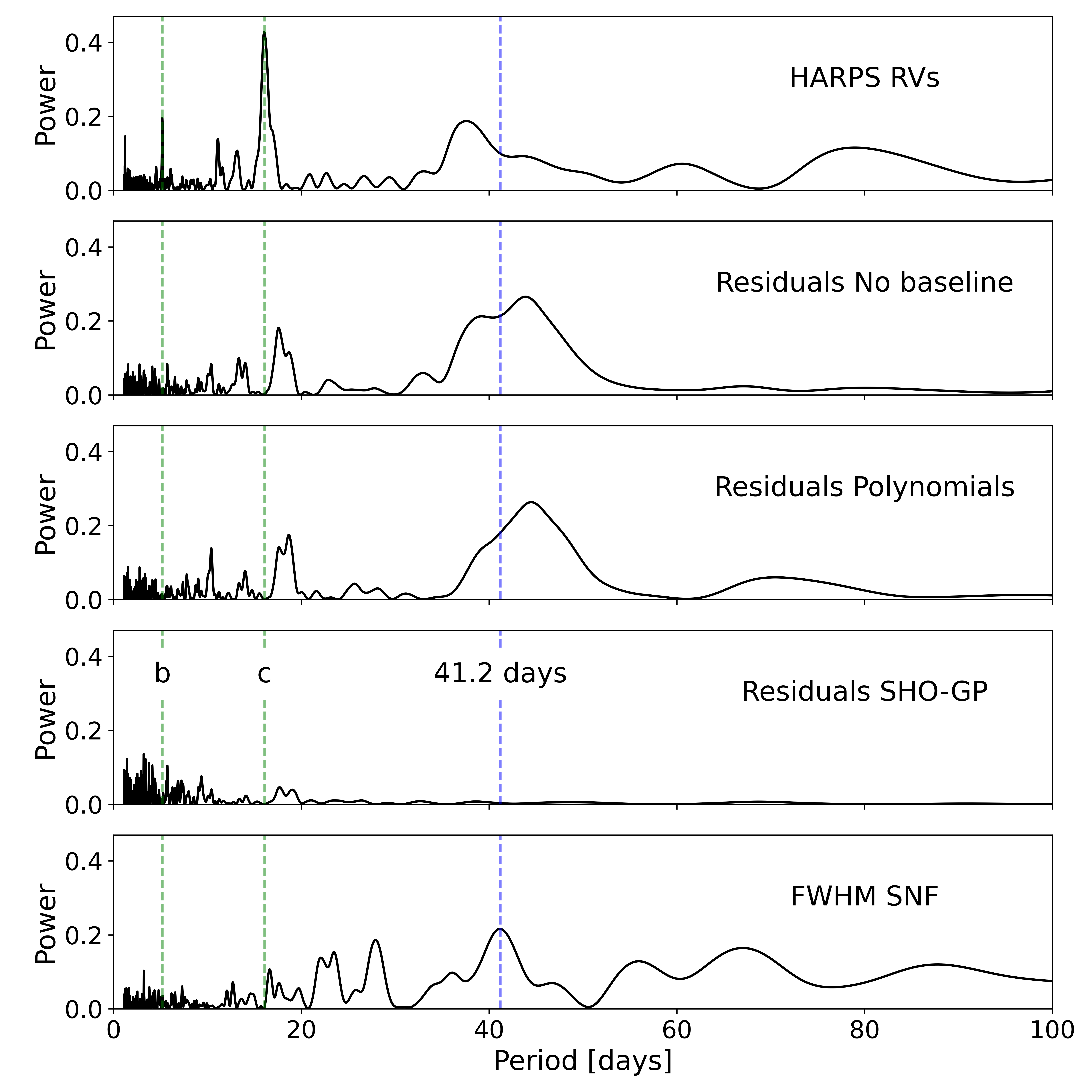
Figure 1: Periodograms of the HARPS SNF data and residuals (i.e. RV - planet signals) when using different baseline models. 1st panel: Raw HARPS SNF data. 2nd panel: Residuals when fitting only for the planetary signals, without any baseline. 3rd panel: Residuals when fitting for the planetary signals and for linear detrending vectors of the activity indicators. 4th panel: Residuals when fitting for the planetary signals and employing a SHO-GP as baseline. 5th panel: FWHM_SN. The dashed green lines represent the orbital periods of the two known planets. The dashed blue line represents the most significant peak in the periodogram of the FWHM_SN activity indicator.

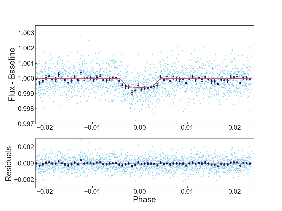
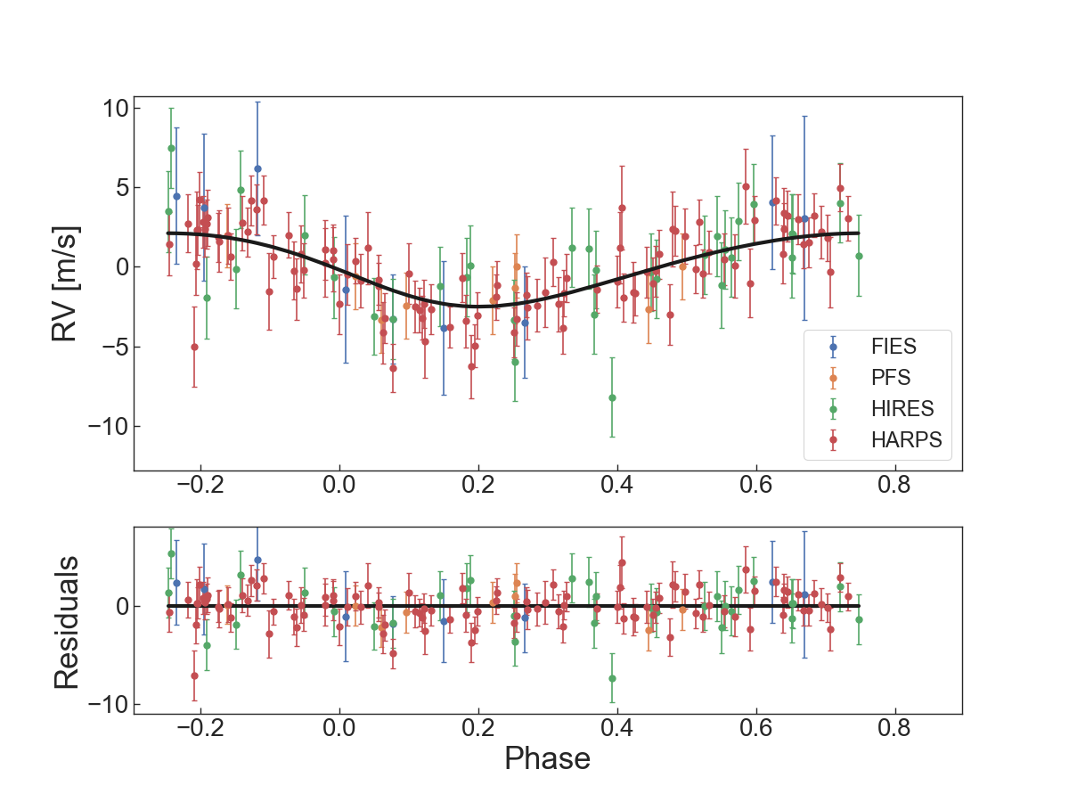
Figure 2: Phase-folded CHEOPS, TESS, and RV data of TOI-421 b. Top panel: Phase-folded and detrended transit light curve of TOI-421 b using four CHEOPS visits. The bright and dark blue points are the original data and the 5-min binned data points, respectively. The red line is the median fitted model and the residuals of the fit are shown in the panel below the light curve. Middle panel: Same as the top panel, but using TESS data observed during Sectors 5, 6, and 32. Bottom panel: Phase-folded and detrended RV data for TOI-421 b using FIES (blue), PFS (yellow), HIRES (green) and HARPS (red). The black line is the median fitted model and the residuals of the fit are shown in the panel below the RV curve. The median fitted model of TOI-421 c has been subtracted from all RV data points.

Figure 3: Same as Figure 2, but for TOI-421 c and using 2 CHEOPS visits.

Table 6: Retrieved planetary and stellar parameters

Parameters	Symbols	Priors	Values	Units
Planet b
Orbital period	$P_{\rm b}$	$\mathcal{U}(5.1975,5.1977)$	$5.197576\pm 0.000005$	days
Transit time	$T_{\rm 0,b}$	$\mathcal{U}(2459189.7,2459189.76)$	$2459189.7341\pm 0.0005$	BJD
Planet-to-star radius ratio	$R_{\rm b}/R_{\star}$	$\mathcal{U}(0.02,0.04)$	$0.0279\pm 0.0008$	-
Impact parameter	$b_{\rm b}$	$\mathcal{U}(0.0,1.1)$	$0.942\pm 0.011$	-
Eccentricity	$e_{\rm b}$	$\mathcal{U}(0.0,1.0)$	$0.13\pm 0.05$	-
Argument of periapsis	$\omega_{\rm b}$	$\mathcal{U}(0,360)$	$140\pm 30$	deg
RV semi-amplitude	$K_{\rm b}$	$\mathcal{U}(1,4)$	$2.83\pm 0.18$	m/s
Transit duration	$\rm dur_{b}$	-	$0.0454\pm 0.0014$	days
Semi-major axis	$a_{\rm b}$	-	$0.0554\pm 0.0010$	AU
Radius	$R_{\rm b}$	-	$2.64\pm 0.08$	$R_{\oplus}$
Mass	$M_{\rm b}$	-	$6.7\pm 0.6$	$M_{\oplus}$
Mean density	$\rho_{\rm b}$	-	$0.37\pm 0.05$	$\rho_{\oplus}$
Equilibrium Temperature	$T_{\rm eq,b}$	-	$922\pm 14$	K
Planet c
Orbital period	$P_{\rm c}$	$\mathcal{U}(16.0672,16.0678)$	$16.067541\pm 0.000004$	days
Transit time	$T_{\rm 0,c}$	$\mathcal{U}(2459195.305,2459195.310)$	$2459195.30741\pm 0.00018$	BJD
Planet-to-star radius ratio	$R_{\rm c}/R_{\star}$	$\mathcal{U}(0.04,0.07)$	$0.0540\pm 0.0006$	-
Impact parameter	$b_{\rm c}$	$\mathcal{U}(0.0,1.1)$	$0.70\pm 0.03$	-
Eccentricity	$e_{\rm c}$	$\mathcal{U}(0.0,1.0)$	$0.19\pm 0.04$	-
Argument of periapsis	$\omega_{\rm c}$	$\mathcal{U}(0,360)$	$102\pm 14$	deg
RV semi-amplitude	$K_{\rm c}$	$\mathcal{U}(3,6)$	$4.1\pm 0.3$	m/s
Transit duration	$\rm dur_{c}$	-	$0.1148\pm 0.0009$	days
Semi-major axis	$a_{\rm c}$	-	$0.1170\pm 0.0018$	AU
Radius	$R_{\rm c}$	-	$5.09\pm 0.07$	$R_{\oplus}$
Mass	$M_{\rm c}$	-	$14.1\pm 1.4$	$M_{\oplus}$
Mean density	$\rho_{\rm c}$	-	$0.107\pm 0.012$	$\rho_{\oplus}$
Equilibrium Temperature	$T_{\rm eq,c}$	-	$635\pm 9$	K
Stellar Parameters
Stellar Density	$\rho_{\star}$	$\mathcal{N}(1.28,0.09)$	$1.28\pm 0.06$	$\rho_{\odot}$
Limb darkening coefficients
CHEOPS passband	$q_{1_{\mathrm{CHEOPS}}}$	$\mathcal{N}(0.487,0.048)$	$0.44\pm 0.04$	-
	$q_{2_{\mathrm{CHEOPS}}}$	$\mathcal{N}(0.359,0.015)$	$0.363\pm 0.010$	-
TESS passband	$q_{1_{\mathrm{TESS}}}$	$\mathcal{N}(0.377,0.040)$	$0.378\pm 0.03$	-
	$q_{2_{\mathrm{TESS}}}$	$\mathcal{N}(0.311,0.015)$	$0.316\pm 0.011$	-
Instrumental Parameters
CHEOPS White-noise	$\sigma_{\rm CHEOPS}$	$\mathcal{U}(6,2500)$	$305\pm 5$	ppm
TESS White-noise	$\sigma_{\rm TESS}$	$\mathcal{U}(17,6740)$	$722\pm 7$	ppm
HARPS Jitter	$\sigma_{\rm HARPS}$	$\mathcal{U}(0.05,135)$	$1.0\pm 0.4$	m/s
HIRES Jitter	$\sigma_{\rm HIRES}$	$\mathcal{U}(0.05,135)$	$2.2\pm 0.4$	m/s
PFS Jitter	$\sigma_{\rm PFS}$	$\mathcal{U}(0.05,135)$	$2.0\pm 0.7$	m/s
FIES Jitter	$\sigma_{\rm FIES}$	$\mathcal{U}(0.001,135)$	$0.02\pm 0.16$	m/s
HARPS offset	$\gamma_{\rm HARPS}$	$\mathcal{U}(-50,50)$	$1.8\pm 0.9$	m/s
HIRES offset	$\gamma_{\rm HIRES}$	$\mathcal{U}(-50,50)$	$-0.8\pm 0.4$	m/s
PFS offset	$\gamma_{\rm PFS}$	$\mathcal{U}(-50,50)$	$2.3\pm 1.3$	m/s
FIES offset	$\gamma_{\rm FIES}$	$\mathcal{U}(-50,50)$	$-7.1\pm 1.3$	m/s
HARPS Amplitude of variations	$\log(S_{0,\rm HARPS})$	$\mathcal{U}(-15,-5)$	$-8.9\pm 0.3$	-
HIRES Amplitude of variations	$\log(S_{0,\rm HIRES})$	$\mathcal{U}(-15,-5)$	$-11.3\pm 1.1$	-
PFS Amplitude of variations	$\log(S_{0,\rm PFS})$	$\mathcal{U}(-15,-5)$	$-9.5\pm 0.8$	-
FIES Amplitude of variations	$\log(S_{0,\rm FIES})$	$\mathcal{U}(-15,-5)$	$-12.3\pm 1.6$	-
RV angular frequency of variations	$\omega_{0,\rm RV}$	$\mathcal{N}(0.153,0.008)$	$0.159\pm 0.007$	1/days
RV Period of variations	$P_{\rm rot,\star}$	$\mathcal{N}(41.2,2.1)$	$39.6\pm 1.6$	days

Figure 4: Stability analysis of the TOI-421 planetary system. For fixed initial conditions (Table 9), the parameter space of the system was explored by varying the orbital period $P_{\mathrm{b}}$ and the eccentricity $e_{\mathrm{b}}$ of planet-b (left panel) and the eccentricities of both planets (right panel). The step size was $10^{-3}$ day in orbital period and $0.0025$ in eccentricity. For each initial condition, the system was integrated over 5000 yr and a stability indicator was calculated, which involved a frequency analysis of the mean longitude of the inner planet. The chaotic diffusion was measured by the variation in the frequency (see text). Red points correspond to highly unstable orbits, while blue points correspond to orbits which are likely to be stable on a billion-years timescale. The black dots show the values of the best fit solution (Table 9).

4.3 Joint analysis

We performed a joint analysis of all photometric and RV datasets using allesfitter. For each of the planets we fitted for the radius-ratio $R_{\rm p}/R_{\star}$, the cosine of the inclination $i$, the term $(R_{\rm p}+R_{\star})/a$, the transit mid-time, the orbital period, the RV semi-amplitude, and the parameters $\sqrt{e}\,\rm cos(\omega)$ and $\sqrt{e}\,\rm sin(\omega)$, which determine the eccentricity $e$ and the argument of periapsis $\omega$.

While using uniform priors for the planetary parameters, we did apply Gaussian priors on the stellar radius and mass according to the values presented in Section 2. This resulted in a prior on the mean stellar density, which in turn constrains the transit model. We also applied a quadratic limb-darkening (LD) law using the parametrisation proposed by Kipping (2013) and used Gaussian priors on the LD coefficients according to theoretically computed values including their uncertainties using the LDCU Python package (see Table 9). LDCU is a modified version of the python routine implemented by Espinoza & Jordán (2015) that computes the LD coefficients and their corresponding uncertainties using a set of stellar intensity profiles accounting for the uncertainties on the stellar parameters. The stellar intensity profiles are generated based on two libraries of synthetic stellar spectra: ATLAS (Kurucz 1979) and PHOENIX (Husser et al. 2013). To check the validity of this additional prior, we performed the same analysis presented here also without constraining the LD coefficients except for their physical boundaries. Although in this case the LD coefficients are only poorly constrained, all of the retrieved planetary parameters are consistent with those presented in this work within their $1\sigma$ confidence intervals.

As discussed in Carleo et al. (2020), the TESS light curves are contaminated by a M dwarf companion (GAIA-ID 2984582227215748224) at an angular distance of $29.4^{\prime\prime}$. The contamination was computed by Carleo et al. (2020) to be $1.8\pm 0.4\%$. The TESS PDSCAP light curves already account for the dilution of the light curve caused by possible contaminants via the contamination estimate in the TESS Input Catalog (TIC). We note that the estimated contamination ratio of 0.0246 is consistent with the value computed by Carleo et al. (2020). Because we used PSF and not aperture photometry for the extraction of the CHEOPS photometry, the CHEOPS data are not affected by contamination.

For the photometric observations, we did fit for an additional white-noise term per instrument. For the RV data, we also added a further jitter-term and a constant offset for each instrument. In terms of baseline models, we used the already detrended CHEOPS data (see Section 4.1) and applied the hybrid spline baseline option in allesfitter to the TESS photometry. As discussed in Section 4.2, for the baselines of the RV data we used a GP with an SHO kernel. While fitting for individual amplitudes of variations $S_{0}$ for each instrument, we jointly fit for a single angular frequency (and therefore period) of variations. We again imposed a prior on this parameter defined by the strongest peak in the periodogram of the FWHM_SN activity indicator in the HARPS SNF data.

The global analysis was performed using the dynamic nested sampling algorithm (e.g. Feroz & Hobson 2008; Feroz et al. 2019) implemented in allesfitter via the dynesty Python package (Speagle 2020). The results of our fit and the successively computed planetary parameters are listed in Table 9. We note that both planetary radii and masses are consistent with the results presented in Carleo et al. (2020) at the $1\sigma$ level. The uncertainties on the radius of both planets decreased by a factor of $\sim 2.5$. Despite the more conservative uncertainty on the stellar mass, the uncertainty on the mass of planet b also decreased. Noteworthy is also the difference in the median values of the transit timing. There is a difference of 74 seconds when comparing the period of planet b as derived by us and as derived by Carleo et al. (2020). This adds up to a difference of 87 minutes ($\sim 1.5$ hours) per year. In the case of planet c, the two periods differ by 56 seconds, which amounts to 21 minutes per year. Considering the prospects of future follow-up spectroscopic observations (see Section 8), these differences of several hours since the publication of the original ephemeris in Carleo et al. (2020) are especially relevant. Finally, we note that we have also been able to significantly detect the eccentricity of both planets, which is especially important in the context of planet formation models and possible observations of the planetary eclipses for atmospheric studies.

4.4 Stability analysis

The TOI-421 system is composed by two close-in low mass planets ($M_{b}\approx 6.7\,M_{\oplus}$, $M_{c}\approx 14.1\,M_{\oplus}$) in moderate eccentric orbits ($e_{b}\approx 0.13$, $e_{c}\approx 0.19$) and near a 3:1 mean motion resonance ($P_{c}/P_{b}\approx 3.091$, Table 9). Because the masses of the planets are in the super-Earth regime, the stability should be assured (eg. Elser et al. 2013). Nevertheless, the significant eccentricity of the planets can introduce many higher order mean motion resonances that can disturb the system.

In order to get a reliable and comprehensive view of the stability of the system, we performed a global frequency analysis (Laskar 1990, 1993) in the same way as achieved for other planetary systems (e.g. Correia et al. 2005, 2010). The system was integrated on a regular 2D mesh of initial conditions in the vicinity of the best fit (Table 9). We used the symplectic integrator SABAC4 (Laskar & Robutel 2001), with a step size of $5\times 10^{-4}$ yr and general relativity corrections. Each initial condition was integrated for 5000 yr, and a stability indicator, $\Delta=|1-n_{b}^{\prime}/n_{b}|$, was computed. Here, $n_{b}$ and $n_{b}^{\prime}$ are the main frequency of the mean longitude of the planet over 2500 yr and 5000 yr, respectively, calculated via the frequency analysis (Laskar 1993). In Figure 4, the results are reported in colour, where orange and red represent strongly chaotic trajectories with $\Delta>10^{-2}$, while extremely stable systems for which $\Delta<10^{-8}$ are shown in cyan and blue. Yellow indicates the transition between the two, with $\Delta\sim 10^{-4}$.

In a first experiment, we explored the stability of the system by varying the orbital period and the eccentricity of the inner planet (Fig. 4, left). We confirm that the best fit solution is stable, despite the existence of some higher order mean motion resonances for eccentricities $e_{b}>0.3$. We also note the presence of a large unstable region at low eccentricity on the right hand side of the figure, corresponding to the 3:1 mean motion resonance. The inner planet is close enough to the star to undergo strong tidal interactions that drive the period ratio to a value above the exact resonance, as it was already reported for many other near resonant systems comprising low-mass planets (e.g. Lissauer et al. 2011; Delisle & Laskar 2014).

As the eccentricity plays an important role in the stability of the system, in a second experiment, we varied the eccentricities of both planets (Fig. 4, right). Though the eccentricities are not very well constrained in the best fit solution (Table 9), we observe that the system is stable as long as $e_{b}\lesssim 0.2$ and $e_{c}\lesssim 0.3$, that is, the system remains stable even if one takes the $3\sigma$ maximum for both eccentricities. We conclude that the TOI-421 planetary system as presented in Table 9 is reliable and resilient to the uncertainties in the determination of the orbital parameters.

5 TTV analysis

Carleo et al. (2020) investigated the possibility of detecting transit timing variations (TTVs). They found an expected TTV signal with a period of $\sim 180$ days and an amplitude of $\sim 4$ minutes. However, they identify two main issues preventing a TTV detection in their analysis: Their photometric baseline covers less than half of the expected TTV period and they observe large uncertainties in the individual transit centre times of the TESS observations ($\sim 1$ minute for the outer and $\sim 4$ minutes for the inner planet). With the addition of a new TESS sector and additional high precision photometric observations by CHEOPS, both issues can be addressed. The photometric baseline now spawns $\sim 1500$ days, although it is sparsely sampled.

To attempt a detection of TTVs we employed a TTV analysis using allesfitter. We fixed the orbital periods and mid-transit times for both planets according to our previously retrieved results. We fitted for the times of all individual transit events by fitting for the differences to the expected transit time. For all other parameters we imposed Gaussian priors according to the values listed in Table 9.

The differences between the observed and calculated mid-transit times are shown in Figure 5. We also re-computed the amplitude of the TTVs, which would be expected for each planet due to the presence of the other planet. For doing this, we used 300 randomly selected posterior samples from the previous joint analysis (see Section 4.3) using the TTVFast code (Deck et al. 2014). The expected TTV amplitude is also shown in Figure 5. We do find hints of TTVs of the order of a few minutes for both planets, however only at low statistical significance. We confirm the observed uncertainties of $\sim 4$ and $\sim 1$ minutes for the TESS observations reported in Carleo et al. (2020). The uncertainty on the transit timing of the first CHEOPS observation of planet b is also $\sim 4$ minutes. The remaining three transit events of planet b observed by CHEOPS still show uncertainties of $\sim 1.5$ minutes, despite the increased photometric precision compared to TESS. Considering also the uncertainty on the linear ephemeris (shown in purple in Figure 5) a statistically significant detection of the expected TTVs would therefore only be possible for the two transit events of planet c observed with CHEOPS, which both show uncertainties of $\sim 22$ seconds. However, both of these observations are consistent with no TTVs within their $1\sigma$ confidence intervals. Therefore, despite the longer photometric baseline and the high photometric precision of the CHEOPS observations, we also fail at statistically significantly detecting the expected TTV signal. Additionally, from the TTV analysis we do not find any evidence supporting the existence of additional planets.

Figure 5: Difference between observed (O) and calculated (C) mid-transit times for TOI-421 b (top) and TOI-421 c (bottom) using observations by TESS (blue) and CHEOPS (green). The red line indicates a difference of zero, which corresponds to no TTVs. The purple lines indicate the $1\sigma$ uncertainties of the linear ephemeris. The red area represents the amplitude of the expected variations considering the dynamical interactions of the two planets as computed from the TTVfast code. See text for further details.

6 Interior structure modelling

Using the results from the joint analysis described in Section 4.3, we inferred the internal structure of both TOI-421 b and c. We followed the procedure introduced in Leleu et al. (2021), which is based on the work of Dorn et al. (2017). In the following, we outline the most important aspects of the used method and present the results.

Our approach uses a full-grid Bayesian inference scheme and models the entire planetary system simultaneously. To make this computationally feasible, we use a deep neural network with six hidden layers trained on our forward model, which models the radius of a planetary structure with a given mass and composition, assuming the planet is spherically symmetric and consists of four fully distinct layers. We use equations of state from Hakim et al. (2018), Sotin et al. (2007), and Haldemann et al. (2020) to model the inner iron core (Fe with up to 19% S), the silicate-rich mantle (Si, Mg, Fe), and a condensed water layer. On top of this structure, we separately model an H-He envelope according to the model of Lopez & Fortney (2014). For the Si/Mg/Fe ratios of the planets, we assume that they match the ones of the host star exactly (Thiabaud et al. 2015).

In our inference scheme, we use priors that are uniform on a simplex for the mass fractions of the iron core, silicate mantle, and water layer, which ensures that they always add up to one. All these mass fractions are calculated with respect to the condensed part of the planet without the H-He envelope. Additionally, we assume a maximal water mass fraction of 0.5 (Thiabaud et al. 2014; Marboeuf et al. 2014). For the H-He layer, our used prior is uniform in log. We note that the results of our analysis do depend to a certain extent on the chosen priors, as this is a highly degenerate problem.

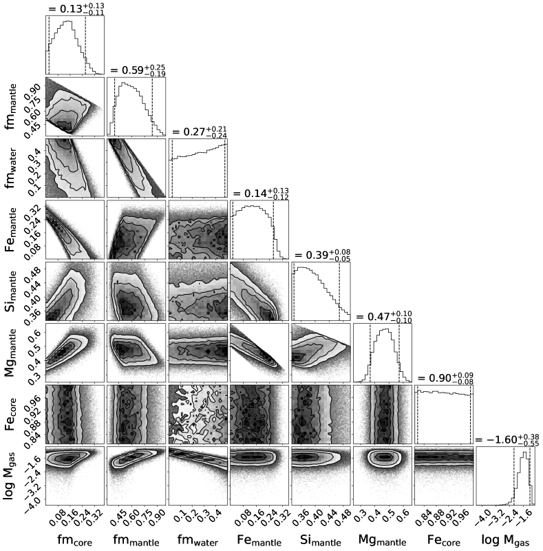
Figure 12: Posteriors of the internal structure parameters obtained for TOI-421 b, namely the inner iron core, silicate mantle, and water layer mass fractions with respect to the condensed part of the planet without the H-He envelope, the molar fractions of Fe, Si, and Mg in the mantle and Fe in the inner core, and the logarithm of the mass of the H-He layer in Earth masses. Each column is labelled with the median of the corresponding posterior, with the 5${}^{\textrm{th}}$ and 95${}^{\textrm{th}}$ percentiles as uncertainties.

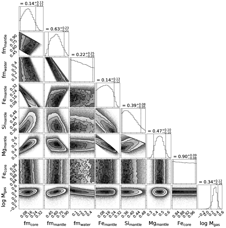
Figure 13: Same as Figure 12, but for TOI-421 c.

The results are visualised in the corner plots in Figures 12 and 13. For both planets, the presence of a water layer remains unconstrained. Meanwhile, the posteriors for the mass and radius of the H-He layer as well as the present-day atmospheric mass fraction show median values of $0.03^{+0.04}_{-0.02}$ $M_{\oplus}$, $0.73^{+0.24}_{-0.22}$ $R_{\oplus}$, and $0.0038\pm 0.0013$ for TOI-421 b and $2.17^{+0.72}_{-0.67}$ $M_{\oplus}$, $2.96^{+0.25}_{-0.25}$ $R_{\oplus}$, and $0.155\pm 0.012$ for TOI-421 c.

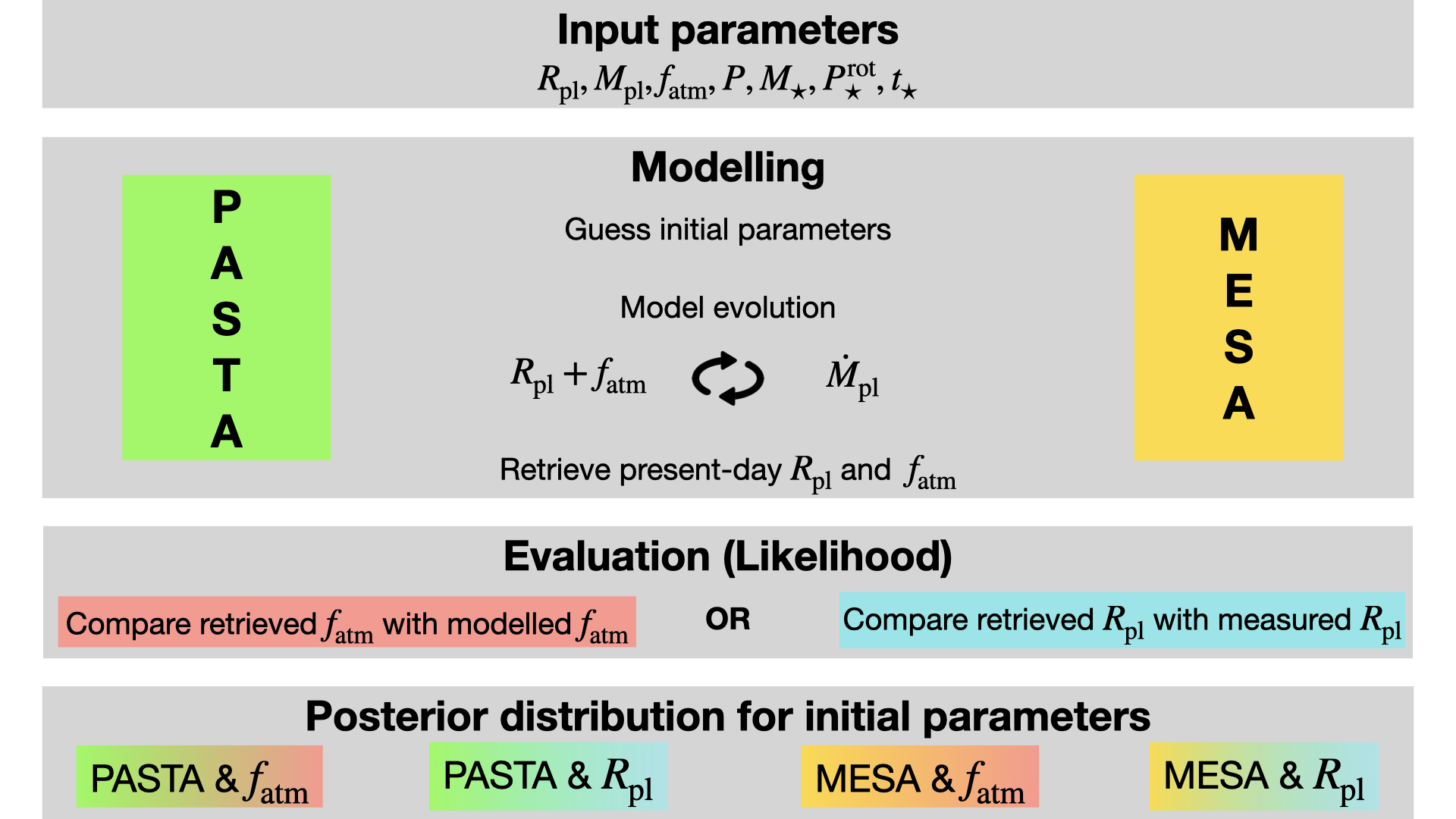
Figure 6: Schematic overview of the different atmospheric evolution modelling approaches compared in this work.

7 Atmospheric evolution

In the following sections (7.1–7.2), we present modelling results of the atmospheric evolution of the planets in the TOI-421 system aiming at constraining their primordial parameters. To have an insight into which physical mechanisms and model assumptions are of particular relevance for such analysis, we employed two different theoretical models and, furthermore, probed two different approaches to fitting the present-day parameters of the planets. First, we employed the Planetary Atmospheres and Stellar RoTation rAtes (PASTA; Bonfanti et al. 2021b) algorithm, which has the advantage of a probabilistic approach enabling one to accurately estimate uncertainties, but omits some of the potentially relevant physics (Section 7.1). For the second model, we employed the framework developed by Kubyshkina & Vidotto (2021); Kubyshkina et al. (2022b) making use of MESA (Modules for Experiments in Stellar Astrophysics; Paxton et al. 2011, 2013, 2018, 2019) to track the thermal evolution and atmospheric structure of the planets (later on referred to as ’MESA-based’ model; Section 7.2). This model includes more advanced physics compared to PASTA, but does not allow one to employ Bayesian statistics due to its long computation time.

In both cases, we run the evolution models attempting to reproduce the present-day parameters of TOI-421 b and c to constrain the primordial parameters of the system (i.e. the free parameters of our models). However, both of our evolution models employ specific atmospheric structure models (relating radius, mass, and atmospheric mass fraction) different from the model presented in Section 6. For PASTA, it is the model based on accretion simulations for pure hydrogen atmospheres by Johnstone et al. (2015b), while MESA relies on physics similar to that of Lopez & Fortney (2014, accounting for thermal evolution) and initial conditions extrapolated from stellar birth lines. Therefore, when fitting for the present-day radii given in Table 9, both evolution models implicitly fit for atmospheric mass fractions different from that given in Section 6, which has been obtained using a more sophisticated structure model. Recent literature (e.g. Delrez et al. 2021; Cabrera et al. 2023) has suggested fitting for the modelled present-day atmospheric mass fractions instead of the radii in order to include the information gained from more sophisticated structure models. In this case, the evolution models implicitly fit for radii different from those obtained from the light curve analysis. In fact, the fitted radii depend on the specific model within the evolution tool that convert $f_{\rm atm}$ into $R_{\rm pl}$. To assess the validity of this alternative approach and identify potential caveats in both approaches, we simulated the evolution for both models once fitting for the observed radii and once fitting for the present-day atmospheric mass fractions from Section 6. Figure 6 provides a schematic overview of the employed workflow and the different model approaches compared in this work. We summarise assumptions and results of each modelling run and fitting approach in Table 7.

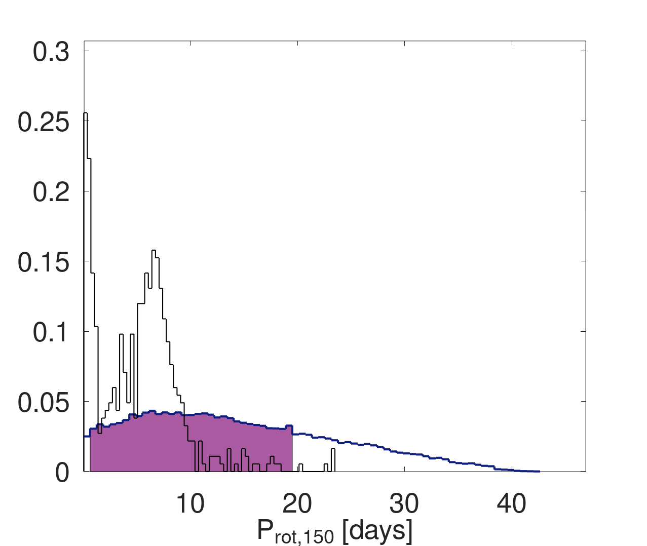
Figure 7: Posterior distribution (dark blue) of the stellar rotation rate of TOI-421 after 150 Myr derived by PASTA. The purple area represents the HPD interval of the distribution. The black line represents the distribution of the stellar rotation rate of young open cluster stars with masses comparable to that of TOI-421 based on the collection of data provided by Johnstone et al. (2015a).

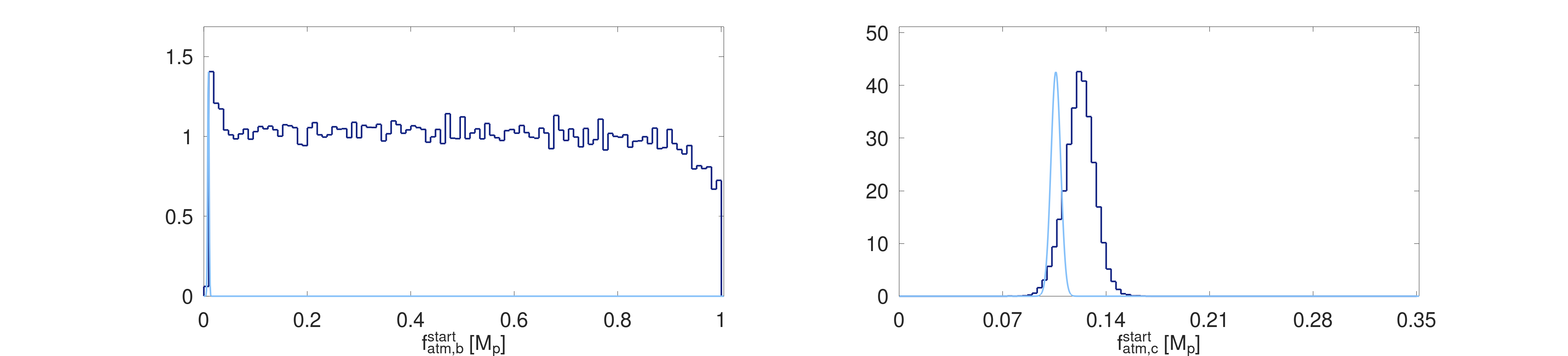
Figure 8: Posterior distribution (dark blue) for the mass of the planetary atmosphere of TOI-421 b (left) and TOI-421 c (right) at the time of the dispersal of the protoplanetary disk derived by PASTA when fitting for the planetary radius (i.e. using the interior structure model by Johnstone et al. (2015b) to convert the observed radius to the present-day atmospheric mass fraction). The light blue line represents the distribution of the estimated present-day atmospheric mass fraction.

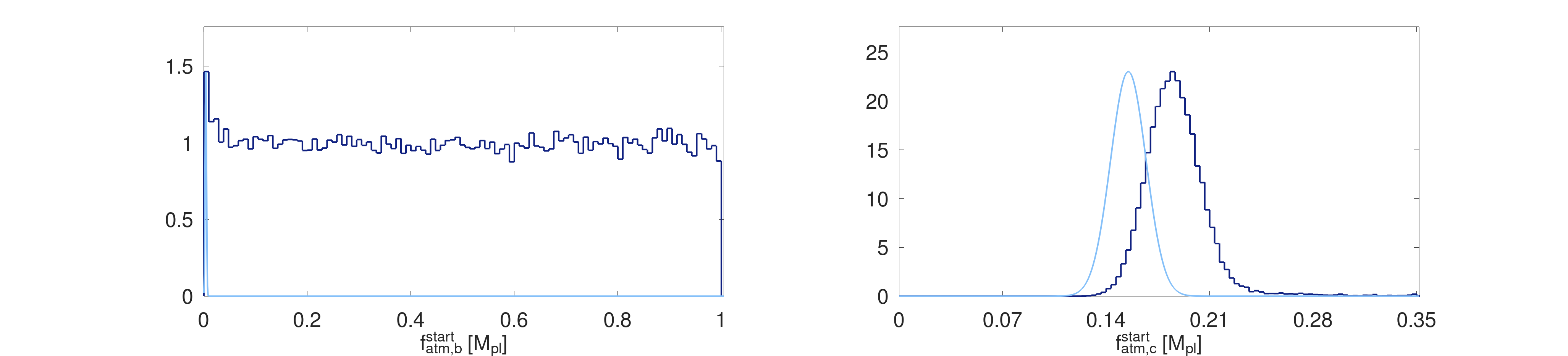
Figure 9: Same as Figure 8, but when fitting for the present-day atmospheric mass fraction (i.e. using the interior structure model described in Section 6 to convert the observed radius to the present-day atmospheric mass fraction).

7.1 Atmospheric evolution with PASTA

PASTA is a planetary atmospheric evolution code based on the original code presented by Kubyshkina et al. (2019a, b). To account for the wide spread in possible stellar rotation rates (hence, L_XUV values) at early ages (e.g. Tu et al. 2015), PASTA simultaneously constrains the evolution of planetary atmospheres and of the stellar rotation rate by combining a model predicting planetary atmospheric escape rates based on hydrodynamic simulations – this has the advantage over other commonly used analytical estimates in that it accounts for both XUV-driven and core-powered mass loss (Kubyshkina et al. 2018) –, a model of the evolution of the stellar XUV flux (using a broken power law to model the evolution of the stellar rotation period; Bonfanti et al. 2021b), a model relating planetary parameters and atmospheric mass (Johnstone et al. 2015b), and stellar evolutionary tracks (Choi et al. 2016).

PASTA works under two main assumptions: (1) planet migration did not occur following the dispersal of the protoplanetary disk; and (2) the planets hosted at some point in the past or still host a hydrogen-dominated atmosphere. The free parameters (i.e. subject to uniform priors) are the planetary initial atmospheric mass fractions at the time of the dispersal of the protoplanetary disk ($f_{\rm atm}^{\rm start}$), which we assume occurs at an age of 5 Myr (see for example Alexander et al. 2014; Kimura et al. 2016; Gorti et al. 2016), and the stellar rotation period at 150 Myr as well as the index of the power law controlling the stellar rotation period of stars older than 2 Gyr, which both are used as a proxy for the stellar XUV emission. The code returns constraints on the free parameters and on their uncertainties by implementing the atmospheric evolution algorithm (for more details on the algorithm see Bonfanti et al. 2021b) in a Bayesian framework (namely the MC3 code Cubillos et al. 2017), using the system parameters with their uncertainties as input priors. PASTA can be set up to either (1) fit the observed planetary radius (e.g. Bonfanti et al. 2021b) or alternatively (2) the modelled present-day atmospheric mass fraction (e.g. Delrez et al. 2021; Cabrera et al. 2023).

As a proxy for the evolution of the stellar rotation period, Fig. 7 displays the posterior distribution (including the high posterior density, HPD) of the stellar rotation period at an age of 150 Myr ($P_{\mathrm{rot,150}}$) when fitting for the present-day atmospheric mass fraction. This distribution is then compared to that of stars member of young open clusters that are of comparable mass extracted from Johnstone et al. (2015a). We find that PASTA is unable to constrain the rotation history of the host star, as indicated by the rather flat posterior distribution. We find an identical result (not shown here) when fitting for the planetary radius instead of the present-day atmospheric mass fraction, which is to be expected as the rotation history of the star is unconstrained and therefore independent of the adopted present-day planetary parameters.

Figures 8 and 9 show the posterior distributions of the initial atmospheric mass fraction for both planets in comparison to the present-day atmospheric mass fraction obtained when fitting for the observed planetary radius and the modelled present-day atmospheric mass fraction, respectively. In both cases PASTA is unable to constrain the initial atmospheric mass fraction of TOI-421 b. For planet c, both approaches return a well-constrained Gaussian posterior distribution for the initial atmospheric mass fraction, indicating that TOI-421 c has lost significant amounts of its primary atmosphere to hydrodynamic escape over the course of its evolution.

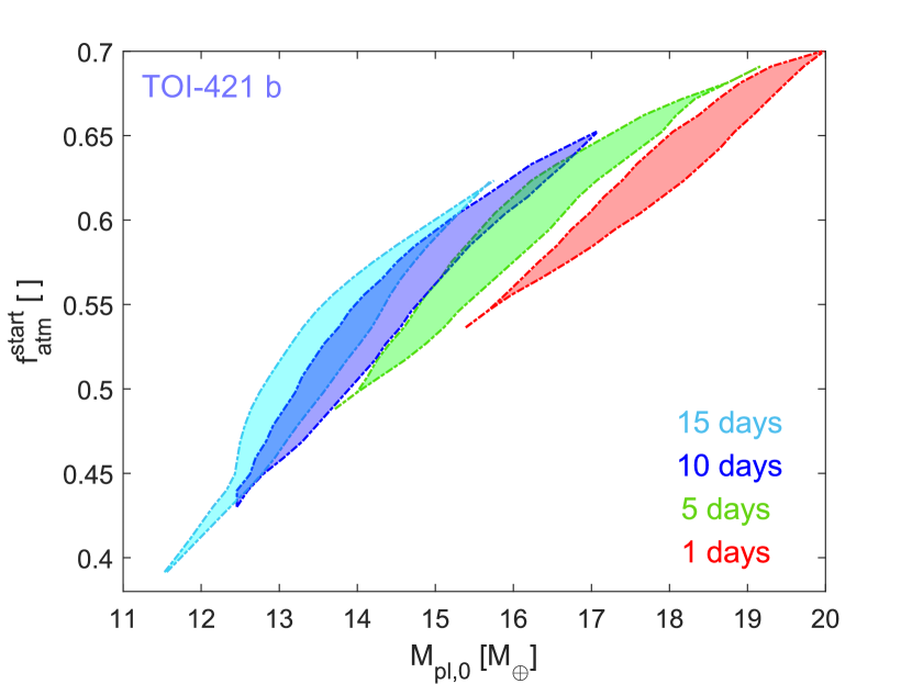
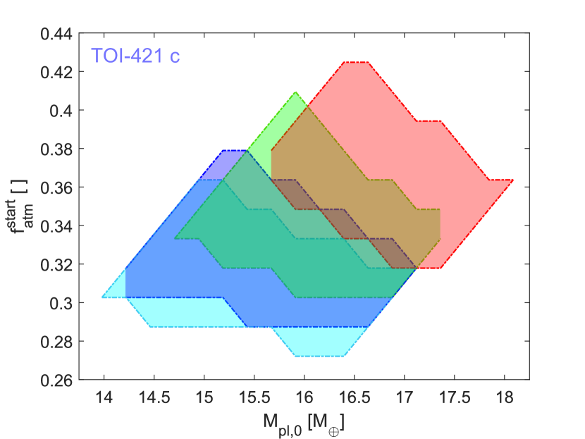
Figure 10: Results of the atmospheric evolution modelling with MESA. Top panel: Initial atmospheric mass fraction against the initial mass of the planet allowing us to reproduce the present-day parameters of TOI-421 b according to our atmospheric evolution models. The admissible combinations of $f_{\rm atm}^{\rm start}$ and $M_{\rm pl,0}$ are shown by the shaded areas, and different colours correspond to different assumptions on the stellar rotation history (i.e. on the rotation period at 150 Myr), as indicated in the legend. Bottom panel: Same as top, but for TOI-421 c.

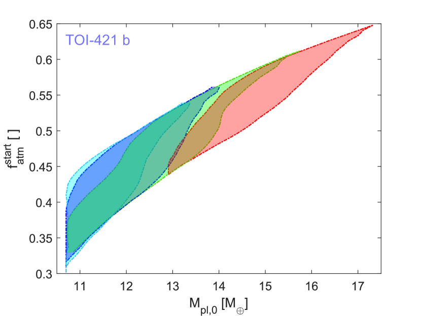
Figure 11: Initial atmospheric mass fraction against the initial mass of the planet allowing us to reproduce the present-day parameters of TOI-421 b (top) and TOI-421 c (bottom) obtained employing the atmospheric mass fraction estimated in Section 6, instead of the observed radius. Notations are the same as in Figure 10.

7.2 Atmospheric evolution based on MESA

As an alternative to PASTA, we also employed the planetary atmosphere evolution model developed by Kubyshkina & Vidotto (2021); Kubyshkina et al. (2022b) relying on the same basic assumptions (no migration and accretion of a primary atmosphere), but employing more sophisticated physics. In detail, the model combines the thermal evolution of a planet hosting a hydrogen-dominated envelope performed with MESA (Paxton et al. 2011, 2013, 2018, 2019) and atmospheric escape based on hydrodynamic modelling (Kubyshkina et al. 2018; Kubyshkina & Fossati 2021) to track the evolution of planetary atmospheric parameters with time. In terms of thermal evolution, the model accounts for both the relaxation of the post-formation luminosity of a planet and changes in planetary equilibrium temperature due to the evolution of the host star. The atmospheric mass loss rates are obtained by direct interpolation on a grid of hydrodynamic upper atmosphere models (Kubyshkina & Fossati 2021).

To account for both the evolution of $L_{\rm XUV}$ and of internal stellar parameters, the model employs the Mors stellar evolution code (Johnstone et al. 2021; Spada et al. 2013). The stellar parameters predicted by Mors for a 0.833 $M_{\odot}$ star at the age of $10.9^{+2.9}_{-5.2}$ Gyr are consistent with the present-day parameters of TOI-421 within $1\sigma$. In terms of X-ray luminosity, the model prediction lies about 15% below the constraint made by (Carleo et al. 2020) based on the $\log{R^{\prime}_{HK}}$ index as outlined in Linsky et al. (2013, 2014); Fossati et al. (2017). For the specific internal parameters of the model, such as planetary core parameters and the lifetime of the protoplanetary disk, we followed the approach used in Kubyshkina et al. (2022b), but these parameters have a minor impact on the results.

As the MESA-based evolutionary model is too computationally expensive to run within a Bayesian framework, for the parameters of the system, we consider either a single value (if the parameter is well constrained, further considering that variations within 1$\sigma$ have a minor impact on the results) or a discrete grid of values (for the key parameters). Thus, we considered single values of stellar mass and orbital separations, but a range of values for the initial stellar rotation rate (controlling $L_{\rm XUV}$) and the initial planetary parameters. Namely, we adopted rotation periods of 1, 5, 10, and 15 days at 150 Myr to span the expected range of stellar rotation periods in young open clusters (see for example Fig. 7). Furthermore, for planet b, we considered initial masses spanning from 10.5 to 24 $M_{\oplus}$ and, for each planetary mass, initial atmospheric mass fractions varying between 15% and 70%. The grid steps for both parameters vary depending on the gradient of the predicted values. Thus, for the planetary mass, the step varies from $0.2$ $M_{\oplus}$ (low-mass end) to $1.0$ $M_{\oplus}$ (at high masses); for the atmospheric mass fraction the step varies between 1% and 5%. For the presentation of the results, we interpolate the outputs onto a regular grid. Differently from Kubyshkina et al. (2022b), we discarded $f_{\rm atm}^{\rm start}$ values above 70%, as they are unlikely from the point of view of formation models. Instead, we extended our grid to lower mass and atmospheric mass fraction values to account for the changes in the observational constraints. For planet c, we considered $M_{\rm pl,0}$ and $f_{\rm atm}^{\rm start}$ lying in the 12.7–22.2 $M_{\oplus}$ and 15–44% range, respectively. The grid steps are 0.2–0.7 $M_{\oplus}$ for the initial mass and 1–2% for the initial atmospheric mass fraction. After performing forward modelling, we checked a-posteriori, which combinations of initial parameters reproduce the estimated present-day planetary properties accounting for their 1$\sigma$ uncertainties.

Table 7: Fitting parameters of the evolution models and their constraints on the initial parameters of TOI-421 system.

Planet	Model	Fitting parameter	$R_{\rm p}$ [$R_{\oplus}$]	$f_{\rm atm}$	$f_{\rm atm}^{\rm start}$	$M^{\rm start}_{\rm p}$ [$M_{\oplus}$]	$f_{\rm atm}^{\rm loss}$ [%]
b	PASTA	$R_{\rm p}$	$\mathbf{2.64\pm{0.08}}$	$0.0087\pm 0.0014$	–	–	–
b	PASTA	$f_{\rm atm}$	$2.32\pm 0.13$	$\mathbf{0.0038\pm{0.0013}}$	–	–	–
c	PASTA	$R_{\rm p}$	$\mathbf{{5.09\pm 0.07}}$	$0.106\pm 0.003$	$0.122\pm 0.010$	$14.4\pm 1.4$	$15\pm 8$
c	PASTA	$f_{\rm atm}$	$6.47\pm 0.7$	$\mathbf{0.155\pm{0.012}}$	$0.19\pm 0.02$	$14.7\pm 1.5$	$22\pm 12$
b	MESA-based	$R_{\rm p}$	$\mathbf{2.64\pm{0.08}}$	$0.026\pm 0.008$	$0.55\pm 0.15$	$14.5\pm 5.0$	$98\pm 2$
b	MESA-based	$f_{\rm atm}$	$2.13\pm 0.13$	$\mathbf{0.0038\pm{0.0013}}$	$0.47\pm 0.17$	$12.6\pm 4.2$	$\sim 99$
c	MESA-based	$R_{\rm p}$	$\mathbf{5.09\pm 0.07}$	$0.242\pm 0.014$	$0.35\pm 0.08$	$16.4\pm 2.6$	$41\pm 21$
c	MESA-based	$f_{\rm atm}$	$4.3\pm 0.2$	$\mathbf{0.155\pm{0.012}}$	$0.23\pm 0.06$	$15.5\pm 2.0$	$39\pm 22$

Figures 10 and 11 summarise our results by showing the $M_{\rm pl,0}$ and $f_{\rm atm}^{\rm start}$ pairs that enable us to reproduce the present-day mass and radius and atmospheric mass fraction assuming different stellar rotation evolution scenarios. At its short orbit, TOI-421 b experiences extreme atmospheric escape with predicted mass loss rates at the present time as high as $\sim 10^{11}-10^{12}$ g s^-1 (Carleo et al. 2020; Kubyshkina et al. 2022a, b; Berezutsky et al. 2022). Therefore, assuming that the planet did not migrate since the time of protoplanetary disk dispersal, we conclude that to achieve its present-day parameters, TOI-421 b had to start its evolution with a mass at least a factor of 1.6 larger than measured and with an initial atmospheric mass fraction larger than 30%, even if the host star evolved as a very slow rotator. There is also a strong correlation between $M_{\rm pl,0}$ and $f_{\rm atm}^{\rm start}$ indicating that the planet has undergone a strong atmospheric boil-off phase at the beginning of its evolution.

Similar to when employing PASTA, we find that TOI-421 c has lost significant amounts of its primordial atmosphere to hydrodynamic escape. However, in the case of the MESA-based models, the escape is expected to be more significant compared to the results of the PASTA models, implying that the planet had a more extensive hydrogen envelope at the beginning of its evolution.

8 Discussion

8.1 Comparison of different atmospheric evolution models

In Section 7, we have employed two different algorithms to simulate the evolution of the primary atmospheres of the TOI-421 planets. The two models mainly differ in the interior structure model they employ to convert atmospheric mass fractions to planetary radii and vice versa. Additionally, the algorithm using the MESA models does also account for planetary thermal evolution and how this affects mass loss, while PASTA does not. Furthermore, they employ different models to follow the evolution of the stellar rotation rate and XUV luminosity. While both models always use their built-in structure models at every step of the evolution, we also tried to constrain the present-day gas-mass by considering the results of a more sophisticated structure model (see Section 6). In these cases, the models fit for the present-day atmospheric mass fraction instead of the observed present-day radius.

In general, we find that the predicted initial atmospheric mass fraction is strongly dependent on the underlying interior structure model used to convert a given planetary radius to an atmospheric mass fraction, and vice versa. When the structure model predicts a higher present-day atmospheric mass fraction, the evolution also results in a higher initial atmospheric mass fraction. This is to be expected as the existence of more gas today presumably implies the existence of more gas at the beginning of the evolution. The relation is however not linear, because a larger amount of gas at any point in time implies a larger planetary radius, and thus a stronger mass loss (Kubyshkina et al. 2020). Therefore we observe that the MESA-based models predict consistently larger initial atmospheric mass fractions than the PASTA models, because its corresponding structure model also results in larger atmospheric mass fractions given the same planetary radii.

With respect to using a modelled present-day atmospheric mass fraction instead of the observed planetary radius to constrain the evolution model (e.g. Delrez et al. 2021; Cabrera et al. 2023), we find that this approach can lead to significantly over- or underestimated planetary radii in the evolution calculations. Since each model always uses its internal structure model to convert atmospheric mass fractions to planetary radii and vice versa at every step of the evolution, this approach forces the model to assume a radius different from the one actually observed in order to match its prediction of an atmospheric mass fraction with the input value. The calculation of a mass loss rate is however strongly dependent on the planetary radius, implying that this approach does not predict consistent mass loss rates during the evolution. Therefore, to employ this approach it is first necessary to check that the interior structure model used in the evolution model returns a radius consistent with the observed one, when providing the atmospheric mass fraction as input.

When converting the observed planetary radius to an atmospheric mass fraction, the more simplistic interior structure models used within our evolution models are not consistent with the more complex interior structure model presented in Section 6. Nevertheless, constraining our evolution models with the results of the more complex interior structure model, also resulted in being inaccurate. Therefore, it appears that none of the model approaches presented in this work are ideal to simulate the atmospheric evolution of this system. Their results may therefore be only considered to be indicative and firm conclusions should be drawn on results that are consistent with all of the approaches. To resolve this issue, new atmospheric evolution models, which use a more complex interior structure model self-consistently, are necessary. Ideally, such a model would also include the possibility to model the presence of volatiles, such as water vapour, in the atmosphere (Burn et al. 2024).

8.2 Planet formation and evolution scenarios of the TOI-421 planetary system

Mordasini (2020) derived a power-law to compute the envelope mass $M_{\rm e,0}$ accreted by a planet while being embedded in the protoplanetary disk as a function of its core-mass $M_{\rm c}$ and orbital separation $a$

$$\frac{M_{\rm e,0}}{M_{\oplus}}=0.024\left(\frac{M_{\rm c}}{M_{\oplus}}\right)^{2.23}\left(\frac{a}{1\rm AU}\right)^{0.72}\,.$$ (2)

This power-law results from fits of corresponding numerical simulations assuming a Sun-like star and a grid of planets with orbital separations ranging from $0.1$ to $1$ AU and core-masses ranging from $1$ to $10\,M_{\oplus}$. Although also being a G-type star, TOI-421 is not exactly Sun-like and with an orbital separation of $\sim 0.055$ AU planet b is also not covered by the grid. Furthermore, the amount of accreted gas is dependent on the lifetime of the protoplanetary disk, with longer disk-lifetimes resulting in more accretion. The disk-lifetime was a free parameter in the simulations of Mordasini (2020) and the derived power-law was then computed on the whole set of simulation results, which had an average disk-lifetime of $2$ Myrs. However, we do not know the real lifetime of the protoplanetary disk of TOI-421, which could be significantly different from $2$ Myrs. Therefore, Equation (2) can just be used to get an order-of-magnitude estimate of the accreted gas-mass.

Employing Equation (2) for both planets using the planetary parameters in Table 9 and assuming that $M_{\rm c}=M_{\rm p}-M_{\mathrm{gas}}$ with $M_{\mathrm{gas}}$ being the present-day gas-mass derived in Section 6, we computed an initial atmospheric mass fraction of $0.030$ and $0.097$ for TOI-421 b and c, respectively. As previously concluded by both Carleo et al. (2020) and Kubyshkina et al. (2022b), we find that TOI-421 b should have lost all of its primary atmosphere to hydrodynamic escape. Even if the planet had accreted a gas-mass an order-of-magnitude larger than estimated by Equation (2) and even if the star had been a very slow rotator, the short orbital separation would have led to enough XUV irradiation to completely strip the planet of its atmosphere. Under the assumptions taken by the evolution models considered in this work, the low measured density of planet b remains an unresolved problem.

In the case of TOI-421 c, we find that all of our atmospheric evolution models result in the planet having had a larger initial atmospheric mass fraction than that predicted by Equation 2. This would imply that similarly to planet b, it is unlikely that planet c formed and evolved hosting a hydrogen-dominated atmosphere at its current orbital separation.

As discussed by Kubyshkina et al. (2022b), the low observed mean density of TOI-421 b might be explained by migration, which implies that the planet formed at a larger orbital separation, where it could have accreted more volatiles. Therefore, following Kubyshkina & Fossati (2022), without migration, a planet born with a primary atmosphere could have the parameters of TOI-421 b in terms of mass and radius if it formed – and evolved – around 0.2–0.3 AU. In a migration scenario, this distance can be seen as a closest-in orbit at which TOI-421 b could have been formed, with the real birthplace located likely further away from the star. In particular, if the planet formed beyond the ice line, a large fraction of its atmosphere would be likely formed or replenished by (partial) melting of the ice in its core (Lopez 2017). In this case, atmospheric evolution would likely be rather different from the case of a pure hydrogen-dominated atmosphere atop a rocky core as considered here, because the available large amount of water vapour in the atmosphere would lead to a more compact atmosphere, significantly reducing atmospheric loss. Furthermore, the addition of a significant amount of heavier species in the atmosphere would lead to additional cooling, and thus lower mass loss (e.g. Johnstone 2020). Additionally, one would also need to employ a different internal structure model (e.g. Aguichine et al. 2021) than the one used in Section 6. If TOI-421 b has been subject to migration, TOI-421 c most likely has migrated as well. As mentioned before, the majority of atmospheric evolution models would require planet c to have accreted significantly more gas than what is predicted by Equation (2). Analogous to planet b, this could also be explained by formation further out compared to the current orbital location and subsequent inward migration of TOI-421 c.

Alternatively, the low density of TOI-421 b might also be explained by the presence of high-altitude clouds (e.g. Lammer et al. 2016; Cubillos et al. 2017; Gao & Zhang 2020). These clouds would bias the measurement of the planetary radius by artificially inflating it compared to that obtained assuming a clear atmosphere. In the case of the Kepler-bandpass (430–880 nm), which is very similar to the CHEOPS-bandpass, a clear hydrogen-dominated atmosphere is opaque in transmission at $\sim 100$ mbar (Lammer et al. 2016; Gao & Zhang 2020), while the presence of aerosols can make the atmosphere opaque already at pressures as low as several nbar. The exact pressure at which the atmosphere becomes opaque is strongly dependent on the atmospheric temperature profile and chemical composition. In order to quantify the possible bias, we use the pressure-temperature profile computed for TOI-421 b by the hydrodynamic model described in Kubyshkina et al. (2018) to determine the height of the $1\mu\rm{bar}$-level, which is a plausible location of high-altitude clouds (Kawashima & Ikoma 2018; Kawashima et al. 2019; Kawashima & Ikoma 2019; Lavvas et al. 2019; Gao & Zhang 2020). Assuming that the atmosphere is opaque below this level, this would imply an overestimation of the planetary radius by 34%. The planetary radius would then be at $\sim 1.97\,R_{\oplus}$, which would in turn result in a mean planetary density of $\sim 0.88\,\rho_{\oplus}$. Using the interior structure model by Johnstone et al. (2015b) built into PASTA this would result in a present-day atmospheric mass fraction of $0.00011$ (i.e. $\sim 98.7\%$ less than when using the observed radius). Additionally, assuming identical relative uncertainties on mass and radius as for the actual measurements (see Table 9), the planet would also be consistent with no H-He atmosphere at all within $1\sigma$, thus allowing for the planet to have formed at its current location without the need of additional orbital migration. Future transmission spectroscopy observations with the James Webb Space Telescope (Gardner et al. 2023) can enable one to explore the atmospheric composition and the existence of high-altitude aerosols, thus constraining the formation and evolution scenarios described above.

9 Conclusion

Using three sectors of TESS data, six CHEOPS visits, and a total of 156 archival radial velocity data points obtained by four different instruments, we derived the mean density of TOI-421 b $0.37\pm 0.05\leavevmode\nobreak\ \rho_{\oplus}$ and TOI-421 c $0.107\pm 0.012\leavevmode\nobreak\ \rho_{\oplus}$, provided updated ephemerides for both planets and a detailed characterisation of the host star. In the process we compared a novel reduction approach for HARPS data, which fits a Skew Normal fit onto the CCFs, with the standard DRS reduced data, finding that results obtained with both approaches are well in agreement with each other. We also attempted to detect TTVs, but concluded that the photometric precision achieved by CHEOPS is not sufficient to statistically significantly detect the expected TTV signal of planet b. In the case of planet c, despite the sufficient precision achieved by CHEOPS, no TTV signal could be identified.

On the basis of the newly retrieved planetary parameters and assuming the presence of a hydrogen-dominated atmosphere, we performed modelling of the interior structure of the planets. We find that under this assumption both planets would have an extensive envelope. Finally, we modelled the evolution of these hydrogen-dominated atmospheres using four different approaches and two different atmospheric evolution models. Independently of the considered model and evolution of the stellar rotation rate, assuming no post-disk migration, we found that TOI-421 b should have completely lost its primary atmosphere. The observed low mean density can therefore not be explained by a formation and subsequent evolution of planet b at its current orbital position. One possible explanation would be a bias in the measured planetary parameters, particularly the planetary radius, as a result of the presence of high-altitude aerosols. Alternatively, the planet might have also undergone orbital migration, including the possibility of a formation beyond the ice line. In this case the atmosphere would no longer be hydrogen-dominated, but most-likely also include a significant amount of water vapour, which would reduce atmospheric loss. A spectroscopic follow-up observation, for example by JWST, has the potential of resolving this dichotomy.

When comparing the different atmospheric evolution approaches used in this work for TOI-421 c, we find that the predicted initial atmospheric mass fraction is strongly dependent on the underlying interior structure model. It ranges between $\sim 10$ and $\sim 35\%$, depending on the considered model and evolution of the stellar rotation rate. While the lower boundary of this range would allow for in situ formation, the majority of solutions would suggest that the planet has also been subject to orbital migration at some point in its evolution. The large range of possible initial atmospheric mass fractions and the fact that no model is clearly more advantageous than the others led us to conclude that results of such models must be reported in ranges rather than in fixed values. It also clearly highlights the necessity of developing new atmospheric evolution models, which use more complex interior structure models self-consistently throughout the modelled evolution, and also account for the presence of volatiles such as water vapour in the atmosphere.

Appendix A Results of internal structure modelling