On the Empirical Complexity of Reasoning and Planning in LLMs

Liwei Kang Zirui Zhao¹¹footnotemark: 1 David Hsu Wee Sun Lee
National University of Singapore
{kang, ziruiz, dyhsu, leews}@comp.nus.edu.sg Equal contribution, listed in alphabetical order.

Abstract

Large Language Models (LLMs) work surprisingly well for some complex reasoning problems via chain-of-thought (CoT) or tree-of-thought (ToT), but the underlying reasons remain unclear. We seek to understand the performance of these methods by conducting experimental case studies and linking the outcomes to sample and computational complexity in machine learning. We found that if problems can be decomposed into a sequence of reasoning steps and learning to predict the next step has a low sample and computational complexity, explicitly outlining the reasoning chain with all necessary information for predicting the next step may improve performance. Conversely, for problems where predicting the next step is computationally hard, adopting ToT may yield better reasoning outcomes than attempting to formulate a short reasoning chain.

Liwei Kang^†^†thanks: Equal contribution, listed in alphabetical order. Zirui Zhao¹¹footnotemark: 1 David Hsu Wee Sun Lee National University of Singapore {kang, ziruiz, dyhsu, leews}@comp.nus.edu.sg

1 Introduction

Reasoning and planning tasks are often challenging due to their inherently multi-step processes. Recently, large language models (LLMs) showed surprising results on reasoning problems when they were asked to explain their reasoning step-by-step through a chain of thought (CoT) Wei et al. (2022) before providing their answers. This was followed by improvements through the use of search algorithms in the tree-of-thought (ToT) Yao et al. (2023); Xie et al. (2023).

Despite these advancements, the conditions for the effectiveness of chain-of-thought and tree-of-thought methods remain unclear. For example, CoT has been very successful in solving grade school math problems, but in the Game of 24, where four numbers need to be manipulated with arithmetic operations to obtain the number 24, CoT provides a solution with a short reasoning chain and fails badly, whereas ToT works reasonably well Yao et al. (2023) (see Fig 1 for CoT and ToT representation of the Game of 24).

We investigate reasoning and planning problems in the context of natural language processing. A reasoning problem entails deducing the answer to a question from provided evidence and applicable reasoning rules. It often requires applying various rules multiple times to connect different pieces of evidence. Planning, a subset of reasoning, requires an action sequence to achieve a desired goal state from a current state. This involves considering available actions and transition functions, which estimate the resultant state from a current state and action. Planning often requires reasoning over a long time horizon, making it computationally harder to solve.

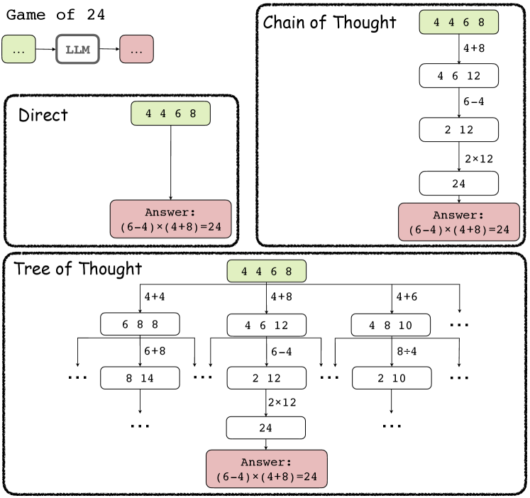
Refer to caption — Figure 1: An illustration of LLM reasoning methods on the Game of 24. Given four poker cards, the player combines the cards using basic arithmetic operations, $(+,-,\times,\div)$ , to reach the target number of 24.

In this paper, we investigate when and why CoT and ToT are effective in reasoning and planning problems from the viewpoint of sample complexity, computational complexity of learning, and computational complexity of reasoning. Sample complexity measures how much data is required for learning. If a learning problem is less complex, as measured by the number of parameters or description length, it correspondingly requires less training data Shalev-Shwartz and Ben-David (2014). This motivates us to analyse the sample complexity of decomposing a problem into multiple steps. Furthermore, learning may become computationally intractable if the values of hidden variables are not observed during learning Aloise et al. (2009); Blum and Rivest (1988), motivating us to consider the presence of hidden variables during learning of chain-of-thought. Finally, for reasoning and planning problems that are computationally hard to solve, e.g. NP-hard problems, it is unlikely that a small predictor producing a short chain of thought that can solve the problem exists in the worst case. This motivates the use of more complex thought structures, e.g., a search tree.

We empirically study these issues through four case studies on grade school mathematics Cobbe et al. (2021), a simple dynamic programming problem Dziri et al. (2023), air travel planning Zhao et al. (2023), and Game of 24 Yao et al. (2023). Common grade school maths problems and the dynamic programming problem we consider have computationally efficient reasoning components. Air travel planning has two different efficient solutions that we compare. Finally, the Game of 24 appears to be computationally difficult.

We study the problems under different settings, including using pre-trained models, fine-tuning, and in-context learning. Our main findings are consistent over the different settings and can be summarized as follows:

•

CoT and ToT can enhance LLM reasoning by lowering the sample complexity through decomposing a problem. In all four cases, decomposition by a chain or tree structure reduces sample complexity and improves performance. In air travel planning, the decomposition with smaller sample complexity performs better.
•

Explicitly annotating all necessary information in predicting the next step can improve CoT performance. In the dynamic programming problem, we show that explicitly demonstrating the relevant variables helps to improve chain-of-thought reasoning further.
•

When finding a short chain solution is computationally hard, a tree structure may be helpful. For tasks like Game of 24, finding a short-chain solution is likely computationally hard, and the tree of thought works substantially better.

These findings suggest a few guiding principles for using LLM to solve reasoning and planning tasks in practice: 1) if simple decomposed problem representations can be found, consider using CoT or ToT, 2) explicitly annotate information required for next-step prediction in the prompts, and 3) use the chain of thought to solve problems in which finding a short chain solution is computationally efficient, otherwise, consider using the tree of thought.

2 Related Works

LLMs have shown significant progress in tackling reasoning and planning problems. Initial studies Wei et al. (2022); Wang et al. (2022); Kojima et al. (2022); Chen et al. (2022); Gao et al. (2023) unveiled various prompting techniques that enable LLMs to demonstrate reasoning processes step by step, thereby substantially boosting their reasoning abilities. This approach has been swiftly adapted to address everyday planning issues Huang et al. (2022a, b); Ahn et al. (2022); Song et al. (2023); Wang et al. (2023); Singh et al. (2023). Subsequent research has integrated LLMs with diverse search algorithms, further enhancing their capability to solve complex reasoning and planning challenges Zhang et al. (2023); Yao et al. (2023); Zhao et al. (2023); Xie et al. (2023); Ding et al. (2023); Feng et al. (2023); Hao et al. (2023); Liu et al. (2023). Nonetheless, a systematic exploration of the conditions under which these methodologies excel or falter is lacking. Our work delves into the empirical principles guiding LLM behaviour across different reasoning frameworks, offering insights into selecting appropriate reasoning strategies for varied task types. While similar efforts Zhao et al. (2023) have discussed different methods’ sample complexity for solving planning problems, they overlook computational implications. One recent study Dziri et al. (2023) discussed the Chain-of-thought’s limitation of compositional reasoning, but they lack a systematic discussion on how to decide the right structure for assembling the reasoning steps. Our research systematically discusses LLM’s capability from the sample complexity and the computational complexity of learning and reasoning.

3 Preliminaries

3.1 Sample and Computational Complexity

We are interested in learning predictors, which take an input, e.g., a sequence of words, and produce a prediction, e.g. a label that may be used directly or as a component of a larger reasoning process. The predictors often have parameters that need to be learned, and for simplicity, we assume that the parameters are discretized with a finite discretization. Instead of the number of parameters, we use a more general notion of description length as a measure of the complexity of a predictor, where the description length is the number of bits required to describe the learnable part of the predictor. Predictors with a small description length can be shown to require less training data, i.e. a small sample complexity Shalev-Shwartz and Ben-David (2014), in order to achieve low generalization error.

Computational complexity is relevant in two ways in this paper: 1) in the amount of computation required for learning, e.g. finding the correct parameters in the predictor given the training data, and 2) in the amount of computation required for reasoning, e.g. finding the solution given a problem after learning.

3.2 LLM reasoning methods

Many LLM reasoning methods have been proposed for performing reasoning using LLMs; we mainly study three representatives and their variants in this paper, namely Direct, Chain-of-thought (CoT), and Tree-of-thought (ToT).

Direct The Direct approach utilizes LLMs to solve reasoning tasks by prompting the model to provide immediate answers. This method may have a low sample complexity if the neural network architecture closely aligns with the reasoning algorithm Xu et al. (2020), meaning a small predictor can effectively represent the algorithm. However, challenges arise when unobserved variables make learning computationally intractable Aloise et al. (2009); Blum and Rivest (1988), though overparameterization might ease learning difficulties Allen-Zhu et al. (2019). Analyzing the alignment between the predictor and algorithm is complex, so we explore a tabular representation for simplicity. In problems with $N$ variables, each taking $K$ values, direct answers require learning a table of size $K^{N}$ , which exponentially increases with more variables. Empirical observations in case studies assess whether the transformer architecture can learn the problem or if it resembles table-filling behaviour.

CoT The Chain-of-thought Wei et al. (2022) method engages LLMs in generating reasoning steps before reaching a conclusion, either by demonstrating these steps in the prompt or by prompting the model “Let’s think step by step” Kojima et al. (2022) at the end of the prompt. CoT often outperforms the Direct approach in reasoning tasks by decomposing problems into actionable components. The LLM extracts or generates actions based on language descriptions or world knowledge, applies these actions through a prediction function (i.e., transition function in planning) to get the next observations, and grounds variable values as needed. With $A$ possible actions, each depending on $a_{i}$ variables, the description length for these actions is proportional to $\sum_{i=1}^{A}K^{a_{i}}$ . We also need a policy function predicting action to select based on observations with its description length of $K^{M}$ if it depends on $M$ variables. If the policy depends only on whether the variables have been observed rather than their values, then a binary table of size $2^{M}$ is sufficient. We use the description length of transition functions and policies as indicators of the sample complexity for decomposed problems.

ToT A tree-of-thought method combines LLMs with a search algorithm, structuring reasoning steps into a tree and selecting promising next steps by self-evaluation. It shows significant improvement in hard problems Yao et al. (2023). Unlike CoT, ToT may not use a policy but relies on an evaluation function for decision-making and a goal recognizer for termination. The complexity of transition functions and the evaluation process in ToT is analyzed similarly to CoT. The computational complexity of solving (versus learning) a reasoning or planning problem becomes a key factor in choosing between CoT and ToT, especially since some problems, e.g. NP-complete problems, have verifiable solutions in polynomial time but are unlikely to have an efficient policy to find solutions. ToT, with its search algorithm, presents a viable solution approach for such hard problems.

We seek to understand the complexity of the problems in the case studies using simple representations. However, LLM learning uses the transformer architecture and is difficult to analyse. Furthermore, the effects of pre-training, which we do not control, are present throughout. Instead, we empirically observe whether the analysis reflects the practical behaviour of the LLMs and whether the insights from analysis are useful in practice, i.e. when analysis suggests that a particular method is preferred, whether it is indeed preferred empirically.

4 Case Studies¹¹1See Appendix A and E for experimental details and complete prompts.

4.1 Grade School Maths

GSM8K Cobbe et al. (2021) consists of grade school math problems described in natural language. It is a real-world problem that LLMs solve very well with CoT Achiam et al. (2023). We investigated a subset of 50 randomly selected problems and discovered that 49 of them can be solved with a chain-style algorithm where, at each step, an equation can be selected such that the values of all variables except one in the equation be known, allowing the value of the remaining variable to be inferred. The remaining problem that cannot be solved this way can be solved using simultaneous equations with two variables, but we ignore this type of problem in the remainder of this study.

4.1.1 Analysis

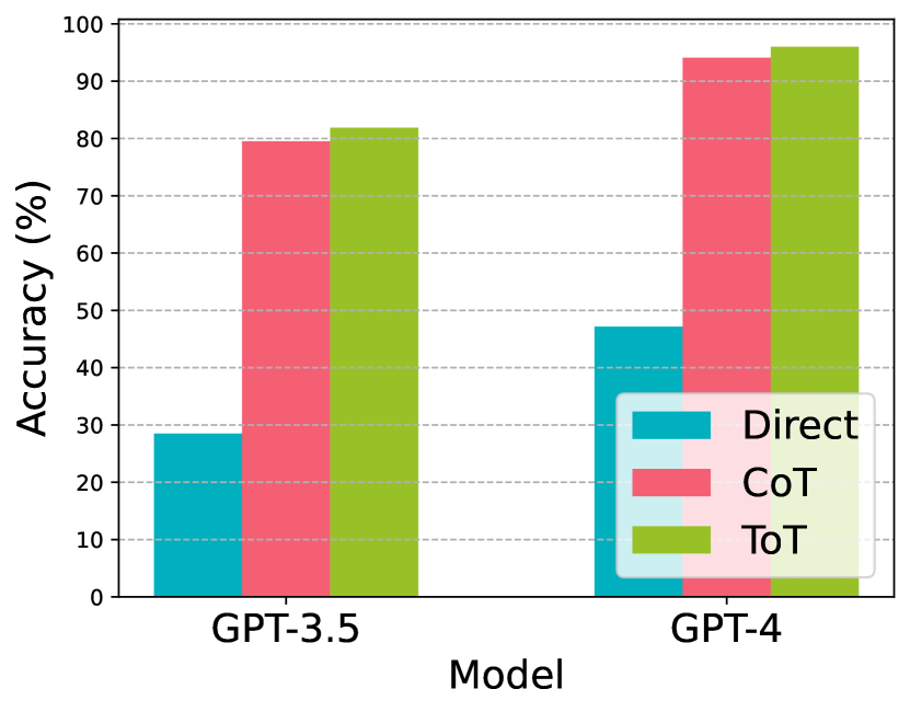
Direct Consider a problem with $N$ variables each can take $K$ values. A tabular representation would require a table of size $K^{N}$ and description length of $O(K^{N}\log K)$ for each question type, assuming each answer also takes $K$ possible values. In the GSM8K dataset, the variable values are usually limited to no more than $6$ digits and the average number of variables per question is $3.93$ . Fig. 2(a) shows that both GPT-3.5 and GPT-4 do not achieve very high accuracy using Direct.

CoT For chain-of-thought (CoT), assuming $A$ different actions whose transition functions require $a_{i}$ variables, the total description length of these operations would be $O(\sum_{i=1}^{A}K^{a_{i}}\log K)$ . In the dataset, the average number of variables in a reasoning step is $2.19$ , so each step is relatively simple. From our analysis, the number of equations that need to be learned as world knowledge appears to be relatively small (see Appendix B.1), and the average number of reasoning steps in the dataset is 3.17. To decide the next equation, we can select an equation where the values of all except one variable are known. There exists a linear time forward chaining algorithm, which we describe in the Appendix B.2, to do that; this translates to a relatively small policy that needs to be learned. These components of the decomposed problems look relatively simple and suggest that decomposition with CoT may be reasonable for this problem. However, the LLM still needs to learn to extract the equations from the question, to learn those that do not appear in the question as world knowledge, and to ground the values of the variables from the previous observations. The LLMs, particularly GPT-4, do remarkably well on GSM8K (see Fig. 2(a)), indicating that extraction and grounding may not be major hurdles for LLMs, which have been trained on large amounts of data. Some errors are still present and are discussed in the Appendix B.3.

ToT We run a beam search ToT, branching after each sentence on the choice of the next sentences suggested by the LLM. We prompt the same LLM to self-evaluate the quality of each proposed reasoning step. As discussed for CoT, there is a simple policy for deciding the next equation to solve, hence search may give limited improvement; this agrees with our experiments as shown in Fig. 2(a).

4.1.2 Fine-tuning Experiments

The GPT experiments suggest that LLMs have difficulties learning to solve GSM type questions directly. To check that, we do fine-tuning experiments with a simplified math word problem. We construct one template word problem with seven variables:

In a zoo, there are $v_{1}$ giraffes. The number of penguins is $v_{2}$ times the number of giraffes, and there are $v_{3}$ times as many monkeys as giraffes. The zoo also has zebras, which are 1/ $v_{4}$ , the number of penguins, and lions, which are 1/ $v_{5}$ , the number of monkeys. If penguins, monkeys, lions, and zebras together make up $v_{6}$ % of the zoo’s total animal population, and elephants constitute $v_{7}$ % of the total, find out how many elephants are there in the zoo.

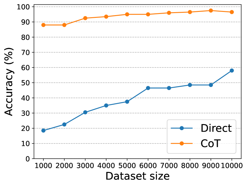
Colored font indicates a variable, the problem is essentially solving one equation: $\text{elephant}=(v_{1}v_{2}+v_{1}v_{3}+v_{1}v_{3}/v_{5}+v_{1}v_{2}/v_{4})v_{7}/v_{6}$ .

We randomly generate 10k configurations of the variables and perform supervised fine-tuning with Direct and CoT with varying amounts of data from 1k to 10k. The results are shown in Fig. 2(b). Note that each CoT example provides substantially more information than each Direct example, but CoT is substantially better even when Direct is provided with 10 times more training examples (Direct at 10k vs CoT at 1k). This suggests that the transformer in the LLM is behaving more like a tabular predictor and is not able to learn to decompose the problem internally without being trained explicitly to do so.

4.2 Dynamic Programming

We study another problem, the Maximum Weighted Independent Set problem (MWIS) Kleinberg and Tardos (2005): Given a sequence of integers, find a subsequence with maximum sum such that no two elements in the subsequence are adjacent in the original sequence. The problem can be solved in linear time using dynamic programming (see Appendix C.1). MWIS was studied in Dziri et al. (2023), showing that LLMs trained on short sequences generalize poorly to longer sequences. In this paper, we focus on the amount of annotation provided in learning where only the answer is provided in Direct, whereas different levels of explicitness in annotation can be provided in CoT.

4.2.1 Analysis

Direct Consider a sequence with $N$ integers; each may take $K$ values. A tabular representation would have $K^{N}$ entries, where each entry needs $N$ bits to indicate the presence of the $N$ number in the subsequence, giving a description length of $O(NK^{N})$ .

CoT Using CoT (see Appendix E.2 for examples), we can see each reasoning step as applying a function to known variables and derive some intermediate results. The function may take up to 3 variables with a constant number of unique functions. We also need a table of size $O(N)$ to indicate which function to use in the next step. The description length of CoT would be $O(K^{3}\log K+N)$ which appears manageable.

4.2.2 In-context Learning

In this section, we will compare prompting LLMs to answer the MWIS problem directly with prompting them to answer using CoT. We will also study two versions of CoT demonstrations and demonstrate that a more explicit demonstration can improve performance substantially.

Consider the following line from the CoT demonstration (see E.3 for the entire demonstration):
Implicit prompt (from Dziri et al. (2023)): … Since dp[0] != input[0] + dp[2] (6 != -4 + 5)
We can make it more explicit as follows:
Explicit prompt: … Since dp[0]=6, input[0]=-4, dp[2]=5, input[0] + dp[2] = 1 != 6 = dp[0]

Both prompts demonstrate steps to use DP to solve the MWIS problem, but in the Implicit prompt, when autoregressively generating the token "!=", the values of dp[0], input[0], dp[2], and input[0]+dp[2] are not explicitly stated in the immediate context and need to be inferred from all previous observations.

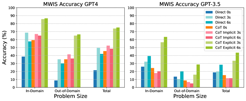
As shown in Fig. 3, making the demonstrations explicit provides more than 20% improvement in many cases compared to the implicit demonstrations from Dziri et al. (2023). This is consistent with the learning problem becoming computationally easier if the relevant variables are made explicit during learning. The sample complexity may also be smaller: the explicit demonstrations is decomposing the single reasoning steps into multiple simpler steps, effectively creating a small chain-of-thought. In contrast to the making the single step a small CoT, we can view deciding between "!=" and "==" in the implicit demonstration as a function of all the previously observed variables. The tabular representation of such a function would have a large description length which suggests that it would require a larger sample complexity to learn.

We observe that prompting LLM to directly give an answer yields performance comparable to the implicit CoT method in Fig. 3. This suggests that while we prompt the LLM to "directly" give an answer, the underlying transformer model is not necessarily learning it by populating a table of size $K^{N}$ as it is unlikely to encounter a very large number of examples of the MWIS problem during pre-training. This suggest that the transformer used in the LLM may align well with the reasoning algorithm used here. We explore this further in fine-tuning experiments.

4.2.3 Fine-tuning Experiments

We perform fine-tuning experiments to study both in- and out-of-domain performance.

To examine the generalizability of the fine-tuned model to OOD examples, we define two types of Domain: 1) Problem size: Fine-tune with problems of sizes 4, 5, and 6. Test with problems of size ranging from 4 to 10. All numbers in the input array are uniformly sampled from $[-100,100]$ 2) Number range: Fine-tune and test with problems of sizes 4, 5, and 6. For fine-tuning data, numbers in the input array are uniformly sampled from $[-100,100]$ , while for OOD test examples, numbers are uniformly sampled from $[-1000,1000]$ .

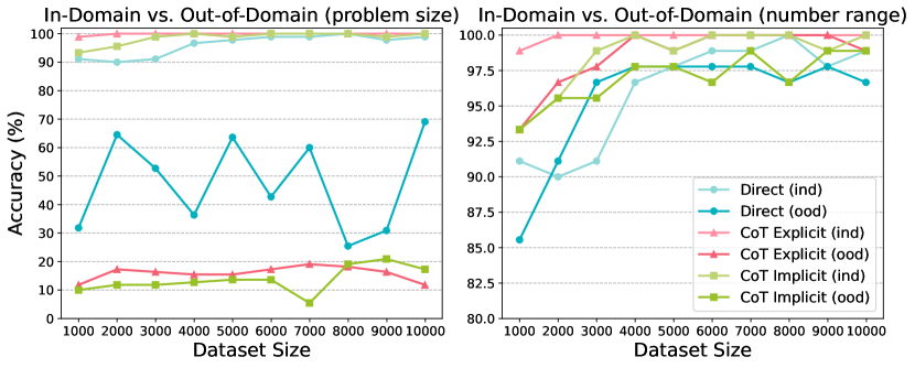
Results For in-domain test examples, we observe that CoT Explicit performs better with the same number of training examples compared with CoT Implicit and Direct. Interestingly, with more fine-tuning data, Direct can achieve performance similar to CoT Explicit. This differs from the math word problem in 4.1.2 where Direct is not comparable with CoT even with ten times more fine-tuning data. Training the transformer to directly approximate the result of this dynamic programming algorithm seems easier than training it to compute the result of a multivariate equation in 4.1.2. But it is unclear whether the difficulty in word math problem is due to computational complexity in learning or poor alignment of transformer with solving that equation; we discuss more about this in Appendix D.

As shown in Dziri et al. (2023), CoT is terrible at generalizing to reasoning length longer than training data, worse than Direct, possibly because LLMs learn by doing pattern matching rather than in a compositional manner Dziri et al. (2023); Kharitonov and Chaabouni (2020). However, all methods exhibit fairly good generalization to different ranges of numbers. In this case, pattern matching may be less of an issue as the structure of the solution remains the same.

4.3 Air Travel Planning

Consider the problem of planning for an air trip: given the starting city and destination, provide the flight route using the direct flights out of each city. For example, if the problem is: What is the flight route from Singapore to New Orleans? One valid answer might be: Singapore-San Francisco-Houston-New Orleans. It is a typical graph search problem: there is an implicit graph where nodes are cities on the earth, and edges are direct flights out of each city. Given a pair of nodes, we aim to find a valid path connecting two graph nodes. To solve this problem, we can either use LLM to predict the flight route directly or use the LLM’s knowledge of the flight graph between cities to conduct a graph search. This problem has been studied in Zhao et al. (2023) using prompting. In this paper, we go further and linearize the graph search algorithm into a CoT, allowing us to study fine-tuning and learning of the graph search algorithm.

4.3.1 Analysis

Assume there are $N$ cities in the domain, and we randomly select two cities as the current and target cities. We first repeat the description length analysis from Zhao et al. (2023), then extend it to a linearized ToT.

Direct & CoT Generating the path directly is essentially the same as CoT as we generate the next city on the path autoregressively. A concise representation of this approach is a table: the row and column of this table are the current city and goal city, and the table entry records the next city to fly to in order to get to the goal. This table has $N^{2}$ entries in total, and each entry takes $\log N$ bits to describe. Thus, the description length of this table is $O(N^{2}\log N)$ bits.

ToT Another method is to use ToT reasoning, in which the LLM acts as the graph, i.e., predicts the direct flight from the current city, together with a hand-coded breadth-first search (BFS) algorithm to find the valid route. Assuming that the total number of edges grows proportionally to the number of cities, describing a sparse graph with $N$ nodes takes approximately $O(N\log N)$ bits, with $\log N$ bits to describe each city in the adjacency list. The graph describes the transition functions; thus, ToT can be described using $O(N\log N)$ bits if the other components are hand-coded. We can linearize the BFS algorithm into a CoT which is entirely generated by the LLM. Other than providing the adjacent cities to each city, the components include being maintaining a first-in-first-out queue, checking whether a city has been visited and recognizing the goal city. For a sparse graph as described, the runtime of BFS is $O(N)$ , which translates to the existence of relatively small predictors for all the functions.

4.3.2 Experiments

Since Direct and CoT are essentially the same, we compare CoT with ToT experimentally. For ToT, the LLM is used only in the expansion step of BFS, when it is queried to generate the neighbour of a city. In addition, we linearize the ToT process into a CoT by generating all the intermediate steps in the BFS computation in ToT-linear.

We use the Kaggle World Cities³³3https://www.kaggle.com/datasets/max-mind/world
-cities-database database data and sample 212 cities with more than 1 million populations. We divide the cities into a large city group (with a population of more than 5 million) and a mid-sized city group (with a population between 1 million and 5 million). We sampled 58 large cities and 154 mid-sized cities. We use the Virtual Radar Server⁴⁴4https://github.com/vradarserver/standing-data to get the real-time (Jan 13, 2024) flight data as the ground truth. We evaluate the settings of travelling between large cities and mid-sized cities.

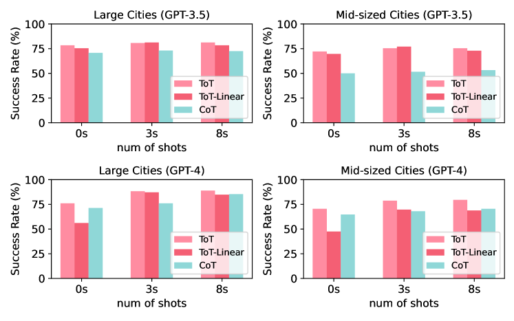
In-context learning The result for in-context learning is shown in Fig. 5. For GPT-3.5, ToT outperforms CoT slightly in large cities and substantially in mid-sized cities. This is consistent with the analysis where the description length of CoT and ToT are $O(N^{2}\log N)$ and $O(N\log N)$ respectively: the gap between CoT and ToT would be larger when $N$ is larger. Surprisingly, ToT-linear is comparable to ToT, even for zero-shot, where the steps in the BFS algorithm are briefly described in the prompt without any examples of its execution, indicating that there is some pre-training of the BFS algorithm in GPT-3.5. GPT-4 generally does better than GPT-3.5 for ToT and CoT, possibly because it has been trained with more data. Interestingly, GPT-4 does not do so well for ToT-linear, particularly for zero-shot, indicating that its pre-training for the BFS algorithm is possibly poorer than GPT-3.5.

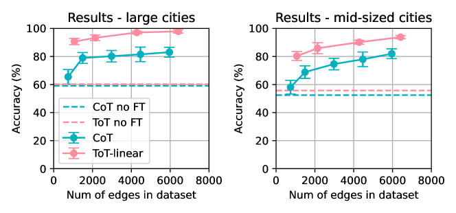
Fine-tuning Experiments In-context learning depends substantially on the pre-training, which we do not control. Fine-tuning allows us to better control the amount of training data used in the experiments. The results of our fine-tuning experiments are in Fig. 6. Each ToT-linear example is longer than a CoT example; hence, we plot the results based on the number of edges observed in training. The results are consistent with the complexity analysis, with ToT-linear performing better than CoT.

4.4 Game of 24

Unlike the above-mentioned problems that can be solved in polynomial time, many puzzle tasks are much harder and unlikely to be efficiently solvable. We use the Game of 24 shown in the introduction: given four numbers, the player must use basic arithmetic operations $(+,-,\times,\div)$ and all four numbers to reach 24. These types of puzzle games are often designed to be hard to solve Kendall et al. (2008), although we are not aware of results on the computational complexity of the Game of 24⁵⁵5A modified version with $N$ rather than four numbers, arbitrary target number instead of 24, and only addition and multiplication with zero allowed is the same as subset-sum, an NP-complete problem. This suggests that similar puzzles are computationally difficult to solve.. The results in Yao et al. (2023), obtained with in-context learning, show that CoT fails while ToT does substantially better. We extend the results by showing that CoT fails in fine-tuning as well, suggesting that the failure is likely due to the mismatch between the computational structure of CoT and the problem. We also consider the decomposition of the actions for in-context learning and show that the decomposition of complex actions into a sequence of simpler actions within a ToT can lead to substantial improvement in performance.

4.4.1 Analysis

We provide a general form of Game of 24 for analysis. Assume $N$ numbers are given, and each number can take $K$ different values. The goal is to use those numbers with arithmetic operations $(+,-,\times,\div)$ to reach $T$ . For the standard Game of 24, $N=4$ , $T=24$ .

Direct Represented as a table, there are $K^{N}$ inputs. A solution is an expression consisting of the $N$ numbers together with $N-1$ operations and corresponding parentheses. Assuming $\log K$ bits to represent numbers, this can be represented using $O(N\log K)$ bits, giving a total table size of $O(NK^{N}\log K)$ bits.

CoT For CoT, the $N-1$ operations are produced in a step-by-step manner. For each step, there are $N(N-1)/2$ ways to select two numbers and 6 distinct operations (both ordering for $-$ and $\div$ , while $+$ and $*$ are symmetric), giving possible $3N(N-1)$ actions. Each operation can be represented with a table with $K^{2}$ entries using $O(K^{2}\log K)$ bits, although pretraining likely has learned these operations for small $K$ . This gives a total description length of $O(N^{2}K^{2}\log K)$ if each action is learned using its own table. If we decompose the selection of two numbers and the arithmetic operation into two steps, then the total description length is $O(N^{2}+K^{2}\log K)$ , and we consider this decomposition in our experiments. Like other computationally difficult problems, there is no simple known policy for selecting the next action. A simple tabular policy would have $O(K^{N})$ entries, and each described using $O(\log N)$ bits.
ToT ToT uses the same actions as CoT but does not need a policy. Instead, we have a goal recognizer and an evaluation function that decides which nodes to expand. Verifying whether a solution is correct can be done in $O(N)$ time, hence a goal recognizer with a small representation exists. Difficult computational problems typically do not have a simple evaluation function; a tabular evaluation function would have $O(K^{N})$ entries. However, a ToT may use a larger computation budget to search a larger part of the search tree when the evaluation function is weaker, compared to CoT, where the next action is selected with a fixed learned policy.

4.4.2 Experiments

As in Yao et al. (2023), we use the hard games indexed 901-1000 from 4nums.com for testing. In our experiments, we consider the output as correct if the expression evaluates to 24 and uses all the input numbers once. To show that it is unlikely that a small chain solution can be easily learned, we fine-tuned Llama-7b-chat with 1200 solution trajectories of Game of 24. Both CoT and Direct failed in all test cases, showing that moderate amounts of data are unlikely sufficient for learning in these settings. For in-context learning, the success rate of the 100 games is reported in Fig. 7.

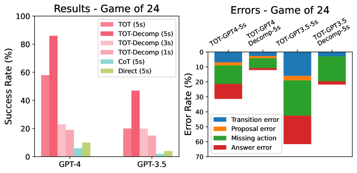
For ToT, we use a beam search with a beam width of 5 and the same action and self-evaluation prompts as Yao et al. (2023). We also constructed a more decomposed version of ToT, ToT-Decomp, where we decompose the action into two steps: the selection of two numbers and the arithmetic operation (see Appendix E.5.1 for examples). Also, ToT-Decomp uses a small CoT that provides the steps for constructing the final equation from the sequence of actions and states in the solution, whereas ToT directly generates the final equation from the action-state sequence.

The results are consistent with those from Yao et al. (2023), with ToT clearly outperforming CoT and Direct. We also find that ToT-Decomp substantially outperforms ToT, demonstrating the advantages of decomposition even within the components of ToT. We perform error analysis as shown in Fig. 7, where we categorize the errors into four types: 1) transition error, where the next state (remaining numbers) is generated incorrectly; 2) proposal error, where the LLM does not generate the correct numbers in the action expression; 3) missing actions, where there are valid actions but not proposed by the LLM; and 4) answer error, where the search is correct but the final expression is incorrect. The results show a substantial reduction in each type of error in ToT-Decomp compared to ToT.

5 Conclusion

This paper introduces a detailed empirical study to understand the effectiveness of chain-of-thought (CoT) and tree-of-thought (ToT) reasoning in planning and reasoning tasks from sample and computational complexity in machine learning. We view the CoT and the ToT as decomposition methods for the underlying problem and study the complexity of the component predictors in the decomposed problems. Our study finds that when the solution can be decomposed as a chain of reasoning steps where predicting the next step is not difficult, explicitly demonstrating the reasoning chain during learning can be helpful. Leaving out important variables for deciding the next reasoning step instead of making all relevant variables explicit in the demonstrations can also make learning more difficult. Finally, when algorithmic analysis indicates that predicting the next reasoning step in a CoT is computationally hard, a ToT structure can be helpful.

Limitations

The suggested methodology from this paper is to analyse the chain-of-thought as a decomposition of the problem and to analyse the complexity of its components. If learning the components has low sample complexity and the computational complexity of predicting the next reasoning step is low, then learning to solve the problem using a chain-of-thought would be reasonable. On the other hand, if the computational complexity of predicting the next reasoning step is high, it may be reasonable to consider learning the components and using a tree-of-thought to solve the problem. This oversimplifies various aspects of the problem. Even though the components have low sample complexity, it may be difficult to learn them in practice as the computational complexity of learning may be high, although this may be alleviated by overparameterization of the predictors used to learn the components. Another issue is out-of-domain generalization. As shown in the MWIS case study, generalization in-domain does not mean that the method will generalize out-of-domain, which may be further exacerbated by overparameterization. Further limitations may apply when doing in-context learning where very few examples are used. Performance may depend heavily on the pre-trained LLM used in this setting. Nonetheless, our case studies suggest that the proposed methodology may still be useful in the in-context learning setting. We would suggest using the guidelines proposed in this paper in a similar way that the Occam Razor principle in the philosophy of science is used. Occam’s Razor suggests that simple explanations for a scientific phenomenon be preferred until shown otherwise by observations. The suggestions we proposed may not work all the time but should similarly be preferred until empirical observations suggest otherwise.

Ethics Statement

This paper studies reasoning and planning in LLMs from a general perspective. While we do not focus on ethics issues, reasoning and planning techniques can potentially be useful in ensuring that AI agents behave ethically through the use of appropriate reward or goal functions that may possibly be learned from data. They may also be used in harmful ways in planning more sophisticated attacks against others. Research on both the use of reasoning and planning for ensuring ethical AI agent behaviour and in mitigating the use of reasoning and planning in performing harmful attacks should be encouraged.

References

Achiam et al. (2023) Josh Achiam, Steven Adler, Sandhini Agarwal, Lama Ahmad, Ilge Akkaya, Florencia Leoni Aleman, Diogo Almeida, Janko Altenschmidt, Sam Altman, Shyamal Anadkat, et al. 2023. Gpt-4 technical report. arXiv preprint arXiv:2303.08774.
Ahn et al. (2022) Michael Ahn, Anthony Brohan, Noah Brown, Yevgen Chebotar, Omar Cortes, Byron David, Chelsea Finn, Keerthana Gopalakrishnan, Karol Hausman, Alex Herzog, et al. 2022. Do as i can, not as i say: Grounding language in robotic affordances. arXiv preprint arXiv:2204.01691.
Allen-Zhu et al. (2019) Zeyuan Allen-Zhu, Yuanzhi Li, and Yingyu Liang. 2019. Learning and generalization in overparameterized neural networks, going beyond two layers. Advances in neural information processing systems, 32.
Aloise et al. (2009) Daniel Aloise, Amit Deshpande, Pierre Hansen, and Preyas Popat. 2009. Np-hardness of euclidean sum-of-squares clustering. Machine learning, 75:245–248.
Blum and Rivest (1988) Avrim Blum and Ronald Rivest. 1988. Training a 3-node neural network is np-complete. Advances in neural information processing systems, 1.
Chen et al. (2022) Wenhu Chen, Xueguang Ma, Xinyi Wang, and William W Cohen. 2022. Program of thoughts prompting: Disentangling computation from reasoning for numerical reasoning tasks. arXiv preprint arXiv:2211.12588.
Cobbe et al. (2021) Karl Cobbe, Vineet Kosaraju, Mohammad Bavarian, Mark Chen, Heewoo Jun, Lukasz Kaiser, Matthias Plappert, Jerry Tworek, Jacob Hilton, Reiichiro Nakano, et al. 2021. Training verifiers to solve math word problems. arXiv preprint arXiv:2110.14168.
Ding et al. (2023) Ruomeng Ding, Chaoyun Zhang, Lu Wang, Yong Xu, Minghua Ma, Wei Zhang, Si Qin, Saravan Rajmohan, Qingwei Lin, and Dongmei Zhang. 2023. Everything of thoughts: Defying the law of penrose triangle for thought generation. arXiv preprint arXiv:2311.04254.
Dowling and Gallier (1984) William F Dowling and Jean H Gallier. 1984. Linear-time algorithms for testing the satisfiability of propositional horn formulae. The Journal of Logic Programming, 1(3):267–284.
Dziri et al. (2023) Nouha Dziri, Ximing Lu, Melanie Sclar, Xiang Lorraine Li, Liwei Jian, Bill Yuchen Lin, Peter West, Chandra Bhagavatula, Ronan Le Bras, Jena D Hwang, et al. 2023. Faith and fate: Limits of transformers on compositionality. arXiv preprint arXiv:2305.18654.
Feng et al. (2023) Xidong Feng, Ziyu Wan, Muning Wen, Ying Wen, Weinan Zhang, and Jun Wang. 2023. Alphazero-like tree-search can guide large language model decoding and training. arXiv preprint arXiv:2309.17179.
Gao et al. (2023) Luyu Gao, Aman Madaan, Shuyan Zhou, Uri Alon, Pengfei Liu, Yiming Yang, Jamie Callan, and Graham Neubig. 2023. Pal: Program-aided language models. In International Conference on Machine Learning, pages 10764–10799. PMLR.
Hao et al. (2023) Shibo Hao, Yi Gu, Haodi Ma, Joshua Jiahua Hong, Zhen Wang, Daisy Zhe Wang, and Zhiting Hu. 2023. Reasoning with language model is planning with world model. arXiv preprint arXiv:2305.14992.
Hu et al. (2021) Edward J Hu, Yelong Shen, Phillip Wallis, Zeyuan Allen-Zhu, Yuanzhi Li, Shean Wang, Lu Wang, and Weizhu Chen. 2021. Lora: Low-rank adaptation of large language models. arXiv preprint arXiv:2106.09685.
Huang et al. (2022a) Wenlong Huang, Pieter Abbeel, Deepak Pathak, and Igor Mordatch. 2022a. Language models as zero-shot planners: Extracting actionable knowledge for embodied agents. In International Conference on Machine Learning, pages 9118–9147. PMLR.
Huang et al. (2022b) Wenlong Huang, Fei Xia, Ted Xiao, Harris Chan, Jacky Liang, Pete Florence, Andy Zeng, Jonathan Tompson, Igor Mordatch, Yevgen Chebotar, et al. 2022b. Inner monologue: Embodied reasoning through planning with language models. arXiv preprint arXiv:2207.05608.
Kendall et al. (2008) Graham Kendall, Andrew Parkes, and Kristian Spoerer. 2008. A survey of np-complete puzzles. ICGA Journal, 31(1):13–34.
Kharitonov and Chaabouni (2020) Eugene Kharitonov and Rahma Chaabouni. 2020. What they do when in doubt: a study of inductive biases in seq2seq learners. In International Conference on Learning Representations.
Kleinberg and Tardos (2005) Jon Kleinberg and Eva Tardos. 2005. Algorithm Design. Addison-Wesley Longman Publishing Co., Inc., USA.
Kojima et al. (2022) Takeshi Kojima, Shixiang Shane Gu, Machel Reid, Yutaka Matsuo, and Yusuke Iwasawa. 2022. Large language models are zero-shot reasoners. Advances in neural information processing systems, 35:22199–22213.
Liu et al. (2023) Jiacheng Liu, Andrew Cohen, Ramakanth Pasunuru, Yejin Choi, Hannaneh Hajishirzi, and Asli Celikyilmaz. 2023. Making ppo even better: Value-guided monte-carlo tree search decoding. arXiv preprint arXiv:2309.15028.
Shalev-Shwartz and Ben-David (2014) Shai Shalev-Shwartz and Shai Ben-David. 2014. Understanding machine learning: From theory to algorithms. Cambridge university press.
Singh et al. (2023) Ishika Singh, Valts Blukis, Arsalan Mousavian, Ankit Goyal, Danfei Xu, Jonathan Tremblay, Dieter Fox, Jesse Thomason, and Animesh Garg. 2023. Progprompt: Generating situated robot task plans using large language models. In 2023 IEEE International Conference on Robotics and Automation (ICRA), pages 11523–11530. IEEE.
Song et al. (2023) Chan Hee Song, Jiaman Wu, Clayton Washington, Brian M Sadler, Wei-Lun Chao, and Yu Su. 2023. Llm-planner: Few-shot grounded planning for embodied agents with large language models. In Proceedings of the IEEE/CVF International Conference on Computer Vision, pages 2998–3009.
Touvron et al. (2023) Hugo Touvron, Louis Martin, Kevin Stone, Peter Albert, Amjad Almahairi, Yasmine Babaei, Nikolay Bashlykov, Soumya Batra, Prajjwal Bhargava, Shruti Bhosale, et al. 2023. Llama 2: Open foundation and fine-tuned chat models. arXiv preprint arXiv:2307.09288.
Wang et al. (2023) Guanzhi Wang, Yuqi Xie, Yunfan Jiang, Ajay Mandlekar, Chaowei Xiao, Yuke Zhu, Linxi Fan, and Anima Anandkumar. 2023. Voyager: An open-ended embodied agent with large language models. arXiv preprint arXiv:2305.16291.
Wang et al. (2022) Xuezhi Wang, Jason Wei, Dale Schuurmans, Quoc Le, Ed Chi, Sharan Narang, Aakanksha Chowdhery, and Denny Zhou. 2022. Self-consistency improves chain of thought reasoning in language models. arXiv preprint arXiv:2203.11171.
Wei et al. (2022) Jason Wei, Xuezhi Wang, Dale Schuurmans, Maarten Bosma, Fei Xia, Ed Chi, Quoc V Le, Denny Zhou, et al. 2022. Chain-of-thought prompting elicits reasoning in large language models. Advances in Neural Information Processing Systems, 35:24824–24837.
Weiss et al. (2021) Gail Weiss, Yoav Goldberg, and Eran Yahav. 2021. Thinking like transformers. In International Conference on Machine Learning, pages 11080–11090. PMLR.
Xie et al. (2023) Yuxi Xie, Kenji Kawaguchi, Yiran Zhao, Xu Zhao, Min-Yen Kan, Junxian He, and Qizhe Xie. 2023. Self-evaluation guided beam search for reasoning. In Thirty-seventh Conference on Neural Information Processing Systems.
Xu et al. (2020) Keyulu Xu, Jingling Li, Mozhi Zhang, Simon S Du, Ken-ichi Kawarabayashi, and Stefanie Jegelka. 2020. What can neural networks reason about? In International Conference on Learning Representations.
Yao et al. (2023) Shunyu Yao, Dian Yu, Jeffrey Zhao, Izhak Shafran, Thomas L Griffiths, Yuan Cao, and Karthik Narasimhan. 2023. Tree of thoughts: Deliberate problem solving with large language models. arXiv preprint arXiv:2305.10601.
Zhang et al. (2023) Shun Zhang, Zhenfang Chen, Yikang Shen, Mingyu Ding, Joshua B Tenenbaum, and Chuang Gan. 2023. Planning with large language models for code generation. arXiv preprint arXiv:2303.05510.
Zhao et al. (2023) Zirui Zhao, Wee Sun Lee, and David Hsu. 2023. Large language models as commonsense knowledge for large-scale task planning. arXiv preprint arXiv:2305.14078.
Zhou et al. (2024) Hattie Zhou, Arwen Bradley, Etai Littwin, Noam Razin, Omid Saremi, Joshua M. Susskind, Samy Bengio, and Preetum Nakkiran. 2024. Understanding length generalization by thinking like transformers. In The Twelfth International Conference on Learning Representations.

Appendix A Experimental Details

All prompting experiments are done with gpt-3.5-
turbo-1106 and gpt-4-1106-preview. All fine-tuning experiments are done with Llama2-7B-chat Touvron et al. (2023) with LoRA $r=64$ , $\alpha=16$ Hu et al. (2021) applied to query and value matrices, and uses $batch\_size=1$ and gradient accumulation steps $=32$ . The template word problem is fine-tuned for 10 epochs with a learning rate of $1e-3$ . MWIS and Game of 24 are fine-tuned for 5 epochs with a learning rate of $3e-4$ . Travel planning is fine-tuned for 300 gradient optimization steps with a learning rate of $3e-4$ . The fine-tuning data is wrapped in the template "<s> [INST] {{prompt}} [/INST] {{completion}} </s>" and the loss is calculated on completion tokens.

Appendix B GSM8K

B.1 Common Rules in GSM8K

We analyzed 50 problems from the GSM8K training set and identified a set of rules. The first five are general rules that can be inferred from the questions and are applicable to multiple problems. The last four are question-specific rules, involving commonsense knowledge that are not mentioned in the questions.

1.

Amount A = Amount B * multiplier
2.

Amount A = Amount B + difference
3.

Total = N_unit * Amount per unit
4.

Total = Sum of components
5.

Current Amount = Initial Amount - Amount Given + Amount Received
6.

Question-specific (implicit): One hour = 60 Minutes
7.

Question-specific (implicit): one sandwich has two slices of bread
8.

Question-specific (implicit): face has two eyes
9.

Question-specific (implicit): 1 quarter = 25 cent; 1 dime = 10 cent; 1 nickel = 5 cent

B.2 An Efficient Algorithm for GSM8K

Based on our analysis of the GSM8K problems in 4.1.1, we give a formulation of the GSM8K problems, and show that there exists an algorithm that has runtime linear to the total input length.

Problem Formulation

Input: A set of $N$ variables $\{V_{1},...,V_{N}\}$ , where the values of some variables are known (from natural language input), while some are unknown (to be inferred); A set of $M$ equations $\{R_{1},...,R_{M}\}$ , where all equations have exactly one variable on LHS; A target variable $V_{t}$ whose value we want to know.

Output: The value of $V_{t}$ .

The solvability of the problem ensures that for all variables, if the value is not given in the natural language question, will appear on the LHS of some equation.

An Efficient Algorithm :

Inspired by Dowling and Gallier (1984), we design an algorithm whose runtime is linear to the size of the problem (total length of all equations).

We maintain a list numvars $[M]$ which stores the number of unsolved variables on RHS for each equation; a list lhslist $[M]$ which stores which variable is on LHS of an equation; a list equationlist $[N]$ which stores the index of the equations where the corresponding variable appears on RHS. We say an equation $R_{i}$ is ready to be processed if numvars $[i]=0$ . We maintain a queue that will contain the equations that are ready to be processed, and it is initialized to contain the equations that are ready to process given the known variables from natural language input.

Then we loop over the queue. Let equation1 be the current head of the queue and let nextvar $=$ lhslist $[$ equation1 $]$ be the variable on the LHS of of equation1. Pop the head of the queue, and iterate over $\texttt{equationlist}[\texttt{nextvar}]$ , for every equation2 in it, reduce $\texttt{numvars}[\texttt{equation2}]$ by $1$ , and if $\texttt{numvars}[\texttt{equation2}]$ becomes $0$ , add equation2 to the queue.

Loop until the queue is empty, we would have solved the values of all $N$ variables. Refer to Algorithm 1 for a more concise representation of the algorithm.

Algorithm 1 Forward Chaining Algorithm for GSM8K Problems

N

variables

\{V_{1},\ldots,V_{N}\}

, with known and unknown values.

M

equations

\{R_{1},\ldots,R_{M}\}

, each with one variable on LHS.

4:Target variable

V_{t}

to find the value of.

6:Value of

V_{t}

7:numvars

[1\ldots M]\leftarrow

Number of unsolved variables on RHS of each

R_{i}

8:lhslist

[1\ldots M]\leftarrow

Variable on LHS of each

R_{i}

9:equationlist

[1\ldots N]\leftarrow

Indices of

R_{i}

where

V_{j}

appears on RHS.

10:Initialize queue readyQueue with indices of

R_{i}

where numvars

[i]=0

11:while readyQueue is not empty do

12:

i\leftarrow

Dequeue from readyQueue.

13:

V_{j}\leftarrow

lhslist

[i]

14: for each

k

in equationlist

[j]

15: numvars

[k]\leftarrow

numvars

[k]-1

16: if numvars

[k]=0

then

17: Enqueue

k

into readyQueue.

18: end if

19: end for

20:end while

21:return Value of

V_{t}

Complexity of the Algorithm numvars and lhslist can be initialized in $O(L)$ , where $L$ is the total length of all equations. When processing an equation, the decrement of numvars corresponds to the "deletion" of occurrences of the variable in an equation, each variable in the equation is looked only once, thus processing all equations also runs in $O(L)$ . Overall, the runtime of the algorithm is $O(L)$ , i.e. linear to the total length of the equations. If we assume each variable appears only once on the LHS of equations, and each equation has a number of variables up to a constant $C$ (as we have seen in 4.1.1, this is often true for GSM8K problems), the runtime of the algorithm would be $O(N)$ , i.e. linear to the number of variables in the problem.

B.3 GSM8K Errors

We observe three types of errors from GPT, namely grounding error, calculation error, and missing rule. We provide an example for each type.

Listing 1: Grounding Error

⬇

Question:

Annie was given a pack of crayons. The pack contained 21 crayons. She already had a box of 36 crayons in her locker. Her friend Bobby gave her half the amount she already had in her locker. She decided to give her sister Mary 1/3 of her total amount of crayons. How many crayons does she give to Mary?

GPT-3.5 response:

"Annie originally had 21 crayons in the pack and 36 crayons in her locker.

So she had a total of 21 + 36 = 57 crayons.

Bobby gave her half the amount she already had, so he gave her 57 / 2 = 28.5 crayons, but since you can’t have half a crayon, let’s round down to 28.

So she now has 57 + 28 = 85 crayons.

So 1/3 of her total amount of crayons is 85 / 3 = 28.33 crayons, but since you can’t have a fraction of a crayon, let’s round down to 28 crayons.

So she gives Mary 28 crayons.

So the answer is 28."

In Listing 1, the problem involves using the rule "Amount A = Amount B * multiplier", which should be grounded as "Amount from Bobby = Amount in Locker * 1/2", not "Amount from Bobby = Amount Annie have in total * 1/2".

Listing 2: Calculation Error

⬇

Question:

To get free delivery, Alice needs to spend a minimum of $35.00 online at her favorite grocery store. In her cart she has 1.5 pounds of chicken at $6.00 per pound, 1 pack of lettuce for $3.00, cherry tomatoes for $2.50, 4 sweet potatoes at $0.75 each, 2 heads of broccoli for $2.00 each and a pound of Brussel sprouts for $2.50. How much more does she need to spend in order to get free delivery?

GPT-3.5 response:

"Alice’s total so far is:

(1.5 * 6) + 3 + 2.50 + (4 * 0.75) + (2 * 2) + 2.50

= 9 + 3 + 2.50 + 3 + 4 + 2 + 2.50

= 26.00

To get free delivery, she needs to spend at least $35.00.

So she needs to spend 35 - 26

= 9.00 more to get free delivery.

So the answer is 9.00."

In Listing 2, the calculation is wrong.

Listing 3: Missing Rule

⬇

Question:

A Ferris wheel can accommodate 70 people in 20 minutes. If the Ferris wheel is open from 1:00 pm until 7:00 pm, how many people will get to ride?

GPT-3.5 response:

"The Ferris wheel can accommodate 70 people in 20 minutes.

There are 6 periods of 20 minutes from 1:00 pm to 7:00 pm.

So in total, the Ferris wheel can accommodate 70 * 6 = 420 people.

So 420 people will get to ride the Ferris wheel from 1:00 pm until 7:00 pm.

So the answer is 420."

In Listing 3, one commonsense knowledge (one hour has 60 minutes) not mentioned in the question is not properly used in the solution.

Appendix C Dynamic Programming

C.1 Algorithm for MWIS

An algorithm that solves the Maximum Weighted Independent Set problem and runs in time $O(N)$ where $N$ is the number of numbers in the input is shown in Algorithm 2.

Algorithm 2 Dynamic Programming Algorithm for the Maximum Weighted Independent Set problem

1:An array

arr

of integers

2:A sequence of decisions maximizing a certain criterion based on

arr

N\leftarrow\text{length of }arr

4:Initialize

dp[0\ldots N-1]

with zeros

dp[N-1]\leftarrow\max(arr[N-1],0)

dp[N-2]\leftarrow\max(arr[N-1],arr[N-2],0)

7:for

i\leftarrow N-3

downto

0

dp[i]\leftarrow\max(dp[i+1],arr[i]+dp[i+2],0)

9:end for

10:Initialize

result

as an empty list

11:

can\_access\_next\_item\leftarrow\textbf{true}

12:for

i\leftarrow 0

N-3

13: if

dp[i]=arr[i]+dp[i+2]

and

can\_access\_next\_item

then

14: Append

1

result

15:

can\_access\_next\_item\leftarrow\textbf{false}

16: else

17: Append

2

result

18:

can\_access\_next\_item\leftarrow\textbf{true}

19: end if

20:end for

21:if

dp[N-2]=arr[N-2]

and

can\_access\_next\_item

then

22: Append

1

result

23:else

24: Append

2

result

25:end if

26:if

dp[N-1]=arr[N-1]

and

can\_access\_next\_item

then

27: Append

1

result

28:else

29: Append

2

result

30:end if

31:return

result

Appendix D Inductive bias of Transformers

From the math word problem and dynamic programming fine-tuning experiments, we see that for some tasks (maximum weighted independent set), the transformer can learn to directly answer the problem efficiently, while for some other tasks (word problem), the direct answer is hard to learn.

We conduct two more experiments to study what might affect the performance of learning to direct answer other than sample complexity: 1) learn the max function, where the input is a list of integers, and the expected output is the maximum value in the input list. This requires only looping over the sequence once, and storing one intermediate value; 2) another dynamic programming problem called rain water⁶⁶6https://leetcode.com/problems/trapping-rain-
water/ that requires looping over the array three times and storing two one-dimensional arrays for memorization. These two problems are similar to MWIS as they all require looping over the input sequence and maintaining some internal variables during the iteration. We use them to study whether the difference between learning to directly answer the template word problem and MWIS is related to the inductive bias of transformers. To eliminate the confounding part, the difficulty of language in the template word problem described in 4.1.2, we perform a modified version of the problem, where we remove all natural language in the prompt. The input would look like "1, 6, 4, 3, 2, 14, 8", and the expected output for this example would be "8".

Task	Accuracy (%)
MWP	58.00
MWIS ( $n\in[4,5,6]$ )	98.89
MWIS ( $n=200$ )	0.01
max ( $n=30$ )	99.50
rain water ( $n=10$ )	89.00

Table 1: Fine-tuning results of different problems. MWP stands for the modified word problem where the input contains only 7 numbers. All tasks are fine-tuned with 10k direct answer examples and evaluated on in-domain examples.

From the results in Table 1, we see that the modified word problem has a similar performance as the original version described in 4.1.2 and Fig. 2(b), which suggests that natural language is not the bottleneck of the template word problem. From the table, we also see that MWIS, max, and rain water perform significantly better than MWP. This suggests that it might be easy for transformers to learn this loop type of problem when the problem size is small. However, when the problem size of MWIS is large ( $n=200$ ), the model fails to generalize to unseen test examples. This aligns with previous findings Weiss et al. (2021); Zhou et al. (2024) that suggest that it would consume one transformer layer to approximate one iteration in an algorithm. And with a problem size of $200$ , it can be hard for transformers to approximate the algorithm in a generalizable way, thus some other patterns in the training set may be exploited, leading to poor generalization.

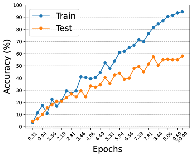
From Fig. 8 we can see that for the template word problem, the transformer can fit the training set reasonably well, while the test set performance peaks at $58.0\%$ . This suggests that by learning to answer directly, the transformer is behaving similarly to learning by filling a table, instead of learning the underlying rational function, which supports our description length analysis.

Appendix E Prompts

E.1 GSM8K Prompts

Listing 4: GSM8K Direct prompt

⬇

direct_8s = """Please answer a math word problem given the following exapmles. Respond only the answer, in the format "The answer is ###."

Example:

Question: There are 15 trees in the grove. Grove workers will plant trees in the grove today. After they are done, there will be 21 trees. How many trees did the grove workers plant today?

The answer is 6.

Question: If there are 3 cars in the parking lot and 2 more cars arrive, how many cars are in the parking lot?

The answer is 5.

Question: Leah had 32 chocolates and her sister had 10 more chocolates than her. If they ate 35, how many pieces do they have left in total?

The answer is 39.

Question: Jason had 20 lollipops. He gave Denny some lollipops. Now Jason has 12 lollipops. How many lollipops did Jason give to Denny?

The answer is 8.

Question: Shawn has five toys. For Christmas, he got two toys each from his mom and dad. How many toys does he have now?

The answer is 9.

Question: There were nine computers in the server room. Five more computers were installed each day, from monday to thursday. How many computers are now in the server room?

The answer is 29.

Question: Michael had 58 golf balls. On tuesday, he lost 23 golf balls. On wednesday, he lost 2 more. How many golf balls did he have at the end of wednesday?

The answer is 33.

Question: Olivia has $23. She bought five bagels for $3 each. How much money does she have left?

The answer is 8.

Question: {question}

The answer is

"""

Listing 5: GSM8K CoT and ToT prompt

⬇

cot_8s = """Please answer a math word problem given the following example. Respond with reasoning steps, and end with the answer, in the format "So the answer is ###."

Example:

Let’s think step by step.

Question: There are 15 trees in the grove. Grove workers will plant trees in the grove today. After they are done, there will be 21 trees. How many trees did the grove workers plant today?

Solution: There are 15 trees originally.

And there were 21 trees after some more were planted.

So 21 - 15 = 6 trees were planted.

So the answer is 6.

Let’s think step by step.

Question: If there are 3 cars in the parking lot and 2 more cars arrive, how many cars are in the parking lot?

Solution: There are originally 3 cars.

And 2 more cars arrive.

So there are 3 + 2 = 5 cars now.

So the answer is 5.

Let’s think step by step.

Question: Leah had 32 chocolates and her sister had 10 more chocolates than her. If they ate 35, how many pieces do they have left in total?

Solution: Originally, Leah had 32 chocolates.

And her sister had 10 more chocolates than her.

So her sister had 42 chocolates.

So in total they had 32 + 42 = 74 chocolates.

Then they ate 35 chocolates.

Therefore they had 74 - 35 = 39 chocolates left.

So the answer is 39.

Let’s think step by step.

Question: Jason had 20 lollipops. He gave Denny some lollipops. Now Jason has 12 lollipops. How many lollipops did Jason give to Denny?

Solution: Jason started with 20 lollipops.

Then he had 12 after giving some to Denny.

So he gave Denny 20 - 12 = 8 lollipops.

So the answer is 8.

Let’s think step by step.

Question: Shawn has five toys. For Christmas, he got two toys each from his mom and dad. How many toys does he have now?

Solution: Shawn started with 5 toys.

And he got 2 toys each from his mom and dad.

So he got 2 + 2 = 4 toys.

Therefore, he has 5 + 4 = 9 toys now.

So the answer is 9.

Let’s think step by step.

Question: There were nine computers in the server room. Five more computers were installed each day, from monday to thursday. How many computers are now in the server room?

Solution: There were originally 9 computers.

And 5 more computers were added from onday to thursday.

There are 4 days between monday and thursday.

So 5 * 4 = 20 computers were added in total.

So there are 9 + 20 = 29 computers now.

So the answer is 29.

Let’s think step by step.

Question: Michael had 58 golf balls. On tuesday, he lost 23 golf balls. On wednesday, he lost 2 more. How many golf balls did he have at the end of wednesday?

Solution: Michael started with 58 golf balls.

And he lost 23 golf balls on tuesday.

So after losing 23 on tuesday, he had 58 -23 = 35.

And then he lost 2 more golf balls on wednesday.

So after losing 2 more on wednesday, he had 35 - 2 = 33 golf balls.

So the answer is 33.

Let’s think step by step.

Question: Olivia has $23. She bought five bagels for $3 each. How much money does she have left?

Solution: Olivia had 23 dollars.

And she bought 5 bagels.

And each bagel costs 3 dollars.

So she spent 5 * 3 = 15 dollars.

So she has 23 - 15 = 8 dollars left.

So the answer is 8.

Let’s think step by step.

Question: {question}

Solution:

"""

Listing 6: GSM8K ToT self-evaluation prompts

⬇

evaluate_prompt = ’’’

Q: Julie climbed 15 steps up the giant slide. She climbed down 6 steps to talk to her friend, Maria. Then she climbed up 8 steps to get to the top. How many steps does the slide have?

Julie climbed 15 steps up.