Robust and tractable multidimensional exponential analysis

H. N. Mhaskar, S. Kitimoon  and Raghu G. Raj, Senior Member IEEE Institute of Mathematical Sciences, Claremont Graduate University, Claremont, CA 91711, U.S.A.. The research of HNM was supported in part by NSF grant DMS 2012355, and ONR grants N00014-23-1-2394, N00014-23-1-2790. email: hrushikesh.mhaskar@cgu.eduInstitute of Mathematical Sciences, Claremont Graduate University, Claremont, CA 91711, U.S.A..
email: sippanon.kitimoon@cgu.edu U.S. Naval Research Laboratory, Washington DC, 20375, U.S.A.. The research of this author is supported in part by the Office of Naval Research (ONR), via 1401091801. email: raghu.g.raj.civ@us.navy.mil
Abstract

Motivated by a number of applications in signal processing, we study the following question. Given samples of a multidimensional signal of the form

f()=k=1Kakexp(i,𝐰k),𝐰1,,𝐰kq,q,||<n,formulae-sequence𝑓bold-ℓsuperscriptsubscript𝑘1𝐾subscript𝑎𝑘𝑖bold-ℓsubscript𝐰𝑘subscript𝐰1formulae-sequencesubscript𝐰𝑘superscript𝑞formulae-sequencebold-ℓsuperscript𝑞bold-ℓ𝑛f({\boldsymbol{\ell}})=\sum_{k=1}^{K}a_{k}\exp(-i\langle{\boldsymbol{\ell}},\mathbf{w}_{k}\rangle),\qquad\mathbf{w}_{1},\cdots,\mathbf{w}_{k}\in\mathbb{R}^{q},{\boldsymbol{\ell}}\in{\mathbb{Z}}^{q},\ |{\boldsymbol{\ell}}|<n,

determine the values of the number K𝐾K of components, and the parameters aksubscript𝑎𝑘a_{k} and 𝐰ksubscript𝐰𝑘\mathbf{w}_{k}’s. We develop an algorithm to recuperate these quantities accurately using only a subsample of size 𝒪(qn)𝒪𝑞𝑛{\cal O}(qn) of this data. For this purpose, we use a novel localized kernel method to identify the parameters, including the number K𝐾K of signals. Our method is easy to implement, and is shown to be stable under a very low SNR range. We demonstrate the effectiveness of our resulting algorithm using 2 and 3 dimensional examples from the literature, and show substantial improvements over state-of-the-art techniques including Prony based, MUSIC and ESPRIT approaches.

Keywords: Exponential sums, localized kernels, digital signal separation.

1 Introduction

Multidimensional exponential analysis is a core problem in signal processing that appears in various applications such as tomographic imaging (including Computerized Tomography (CT), magnetic resonance imaging (MRI), radar and sonar imaging), wireless communication, antenna array processing, sensor networks, and automotive radar, among others. Mathematically, the problem can be formulated as follows. Given a multidimensional signal of the form

f(𝐱)=k=1Kakexp(i𝐱,𝐰k),𝐱,𝐰1,,𝐰kq,formulae-sequence𝑓𝐱superscriptsubscript𝑘1𝐾subscript𝑎𝑘𝑖𝐱subscript𝐰𝑘𝐱subscript𝐰1subscript𝐰𝑘superscript𝑞f(\mathbf{x})=\sum_{k=1}^{K}a_{k}\exp(-i\langle\mathbf{x},\mathbf{w}_{k}\rangle),\qquad\mathbf{x},\mathbf{w}_{1},\cdots,\mathbf{w}_{k}\in\mathbb{R}^{q}, (1.1)

find the number K𝐾K of components, and the parameters aksubscript𝑎𝑘a_{k} and 𝐰ksubscript𝐰𝑘\mathbf{w}_{k}’s. Of course, this is a problem of inverse Fourier transform if we could observe the function f𝑓f at all values of 𝐱𝐱\mathbf{x}. In practice, however, one can observe (after some sampling and renaming of the variables) the values of f𝑓f at only finitely many multi-integer values of 𝐱𝐱\mathbf{x}. In this case, it is not possible to distinguish values of 𝐰ksubscript𝐰𝑘\mathbf{w}_{k} which are equal modulo 2π2𝜋2\pi in all variables. So, this is a special case of the ancient trigonometric moment problem [18], except that we do not have all the trigonometric moments (i.e., the samples f()𝑓bold-ℓf({\boldsymbol{\ell}})) for all values of qbold-ℓsuperscript𝑞{\boldsymbol{\ell}}\in{\mathbb{Z}}^{q}. Thus, the problem is the ill-posed problem known often as the super-resolution problem: knowing the information in a finite domain of the frequency space, we need to extend it to the entire frequency space. The important problem in this connection is to determine the relationship between the number of samples f()𝑓bold-ℓf({\boldsymbol{\ell}}) needed to recuperate the desired quantities up to a given accuracy.

Over the past several decades, several approaches to exponential analysis have been investigated. These can be categorized in three main groups–Fourier based, Prony based, and subspace based methods.

  • Fourier-based methods: In order to utilize Fourier-based methods, it is necessary to obtain a substantial and densely sampled dataset in either a two-dimensional (2D) or three-dimensional (3D) format. However, the collection of such a dataset can be time-consuming. Additionally, these techniques face a trade-off between time and frequency resolution, making it challenging to distinguish closely located scatterers, as pointed out in reference [5].

  • Prony’s methods: Prony’s spectral estimation or exponential analysis algorithms have attracted the interest of numerous researchers. In reference [14], the authors assert that these methods exhibit significantly higher accuracy compared to Fourier-based approaches. However, it is important to note that the effectiveness of exponential analysis techniques can be substantially compromised when dealing with a low signal-to-noise ratio (SNR), resulting in the misclassification of noise as actual signals. There are many recent efforts to stabilize the Prony method by taking more than the minimal number of samples. The number of samples required to recuperate the 𝐰ksubscript𝐰𝑘\mathbf{w}_{k}’s up to an accuracy of 𝒪(1/n)𝒪1𝑛{\cal O}(1/n) is typically on the order of O(nq)𝑂superscript𝑛𝑞O(n^{q}) [4, 8, 11, 13], O(2qn)𝑂superscript2𝑞𝑛O(2^{q}n) [16], O(nlogq1n)𝑂𝑛superscript𝑞1𝑛O(n\log^{q-1}n) [5], or at most (q+1)n2log2q2n𝑞1superscript𝑛2superscript2𝑞2𝑛(q+1)n^{2}\log^{2q-2}n [17].

  • Subspace methods: Under the rubric of target estimation or localization, which is one of the fundamental problems in radar signal processing with many civilian and military applications including landmine detection and geolocations (cf. [20]), a broad set of techniques has emerged for solving exponential analysis problems. Most of these methods are categorized broadly as subspace methods [7], and are based on statistical considerations, rather than the nature of the signal itself. In fact, quite a few papers, e.g., [19, 15], are interested in testing a statistical hypothesis on whether or not there exists a signal at all. There is a theoretical limit on how much SNR can be tolerated, depending upon the number of antenna elements and number of observations [19], in spite of a huge computational cost. On the other hand, beamforming methods [7] take into account the nature of the signal but focus again on noise, and try to maximize the SNR.

In [3, 2], the authors proposed a method to solve the problem using a combination of Prony and subspece based methods, so that number of sample required is 𝒪(n)𝒪𝑛{\cal O}(n). Our paper develops these ideas further to develop an algorithm that also utilizes 𝒪(qn)𝒪𝑞𝑛{\cal O}(qn) samples, but is far more robust under noise. Our method is based on localized trigonometric polynomial kernels developed in [9]. In contrast to the subspace based methods, our method takes into account the nature of the signal, resulting in a significant noise reduction with only a small number of observations per signal, and yields accurate results with theoretical guarantees. This is a completely different viewpoint from what we have seen in the literature, and therefore, not entirely comparable with other approaches.

The rest of this paper is organized as follows. Section 2 introduces the system model for tomographic imaging which illustrates how the problem of multidimensional exponential analysis arises in signal processing. In Section 3, we introduce the concept of localized trigonometric kernels, and provide the neccessary probabilistic background to formulate the main results of our paper which we state and prove our main results in Section 4. The algorithms to implement these theorems are given in Section 5, and demonstrated in the case of the three examples explored in [3].

2 System model

In this section, we explain how the problem of multidimensional exponential analysis arises in tomographic imaging.

In tomographic imaging, an object of interest being imaged is probed by a sequence of monochromatic tones is swept through a frequency range [Ωinit,Ωfin]subscriptΩ𝑖𝑛𝑖𝑡subscriptΩ𝑓𝑖𝑛[\Omega_{init},\Omega_{fin}]. The sensor transmits a signal onto a scene with respect to various angles {𝜽m=(θm,ϕm)}msubscriptsubscript𝜽𝑚subscript𝜃𝑚subscriptitalic-ϕ𝑚𝑚\{{\boldsymbol{\theta}}_{m}=(\theta_{m},\phi_{m})\}_{m}, where θm[Θinit,Θfin]subscript𝜃𝑚subscriptΘ𝑖𝑛𝑖𝑡subscriptΘ𝑓𝑖𝑛\theta_{m}\in[\Theta_{init},\Theta_{fin}] and ϕm[Φinit,Φfin]subscriptitalic-ϕ𝑚subscriptΦ𝑖𝑛𝑖𝑡subscriptΦ𝑓𝑖𝑛\phi_{m}\in[\Phi_{init},\Phi_{fin}]. The scene itself is modeled as a distribution, μ𝜇\mu, which is a linear combination of weighted and spatially shifted Dirac delta functons of dimensionality q𝑞q. For the case of 3D imaging, q=3𝑞3q=3; i.e., μ𝜇\mu is supported on a cube–consisting of points r=[r1,r2,r3]T𝑟superscriptsubscript𝑟1subscript𝑟2subscript𝑟3𝑇r=[r_{1},r_{2},r_{3}]^{T}, for 1r1D11subscript𝑟1subscript𝐷11\leq r_{1}\leq D_{1}, 1r2D21subscript𝑟2subscript𝐷21\leq r_{2}\leq D_{2}, and 1r3D31subscript𝑟3subscript𝐷31\leq r_{3}\leq D_{3}–whose side-lengths (D1𝐷1D1, D2𝐷2D2, and D3𝐷3D3) are referred to as the dimensions of the scene reflectivity function.

We define the center reference point (CRP) to be the center of mass of the scene to be reconstructed, and the line of sight (los) as the unit vector that points from the transmitter to the CRP of the scene. The distance along the los from the transmitter to the range-bin, 𝐫0subscript𝐫0\mathbf{r}_{0}, of interest is called the ‘downrange’ r0=𝐫0subscript𝑟0normsubscript𝐫0r_{0}=\|\mathbf{r}_{0}\|. Given this, it can be shown that the backscattered signal at downrange 𝐫0subscript𝐫0\mathbf{r}_{0} from the sensor, when viewed at angle 𝜽𝜽{\boldsymbol{\theta}}, is given by

Υ(t)|𝜽,𝐫0=[R𝜽{μ}(r0)]χ(t2r0νp)+(t),evaluated-atΥ𝑡𝜽subscript𝐫0delimited-[]subscript𝑅𝜽𝜇subscript𝑟0𝜒𝑡2subscript𝑟0subscript𝜈𝑝𝑡\Upsilon(t)|_{{\boldsymbol{\theta}},\mathbf{r}_{0}}=[R_{{\boldsymbol{\theta}}}\left\{\mu\right\}(r_{0})]\chi\left(t-\frac{2r_{0}}{\nu_{p}}\right)+\aleph(t), (2.1)

where 2r0/νp2subscript𝑟0subscript𝜈𝑝2r_{0}/\nu_{p} denotes the two-way time delay, νpsubscript𝜈𝑝\nu_{p} represents the speed of wave propagation, (t)𝑡\aleph(t) is the measurement noise, and R𝜽subscript𝑅𝜽R_{{\boldsymbol{\theta}}} is the Radon transform of the scene, μ𝜇\mu, with respect to angle 𝜽𝜽{\boldsymbol{\theta}}, and evaluated at the downrange location r0subscript𝑟0r_{0}. This corresponds to the integral across sensor returns from all points along a hyperplane perpendicular to the downrange location r0subscript𝑟0r_{0}, commonly referred to as an ‘iso-range contour’.

Therefore the complete response at time t𝑡t from all ranges, along the line formed by intersecting the scene at 𝜽𝜽{\boldsymbol{\theta}}, is rewritten as

Υ𝜽(t)=[R𝜽{μ}(r)]χ(t2rνp)𝑑r+(t).subscriptΥ𝜽𝑡delimited-[]subscript𝑅𝜽𝜇𝑟𝜒𝑡2𝑟subscript𝜈𝑝differential-d𝑟𝑡\Upsilon_{{\boldsymbol{\theta}}}(t)=\int[R_{\mathbf{{\boldsymbol{\theta}}}}\left\{\mu\right\}(r)]\chi\left(t-\frac{2r}{\nu_{p}}\right)\,dr+\aleph(t). (2.2)

This can be reformulated in convolution form (after a choice of units, without loss of generality, so that νp=2subscript𝜈𝑝2\nu_{p}=2) as:

Υ𝜽(t)=(R𝜽(μ)χ)(t)+(t),subscriptΥ𝜽𝑡subscript𝑅𝜽𝜇𝜒𝑡𝑡\Upsilon_{{\boldsymbol{\theta}}}(t)=\left(R_{{\boldsymbol{\theta}}}(\mu)\ast\chi\right)(t)+\aleph(t), (2.3)

where \ast denotes the convolution operation. Equation (2.3) can be interpreted as the response to an Linear Time Invariant (LTI) system with an input signal χ(t)𝜒𝑡\chi(t) and an impulse response μ𝜽(t)subscript𝜇𝜽𝑡\mu_{{\boldsymbol{\theta}}}(t) which characterizes the interaction between the transmit waveform and the scene with respect to sensing angle 𝜽𝜽{\boldsymbol{\theta}}. The received signal Υ𝜽(t)subscriptΥ𝜽𝑡\Upsilon_{{\boldsymbol{\theta}}}(t), is the output of this LTI system and is subsequently sampled at the receiver. Given Υ𝜽(t)subscriptΥ𝜽𝑡\Upsilon_{{\boldsymbol{\theta}}}(t) for a finite grid 𝜽{𝜽m}𝜽subscript𝜽𝑚{\boldsymbol{\theta}}\in\{{\boldsymbol{\theta}}_{m}\} as described earlier, our problem is to estimate the underlying scene reflectivity function μ𝜇\mu i.e. to form the image. In this paper we consider the basic case where χ(t)=δ(t)𝜒𝑡𝛿𝑡\chi(t)=\delta(t), where δ(t)𝛿𝑡\delta(t) is the Dirac delta function. In this case, the received signal at angle 𝜽𝜽{\boldsymbol{\theta}} is given by

Υ𝜽(t)=R𝜽(μ)(t)+(t).subscriptΥ𝜽𝑡subscript𝑅𝜽𝜇𝑡𝑡\Upsilon_{{\boldsymbol{\theta}}}(t)=R_{{\boldsymbol{\theta}}}(\mu)(t)+\aleph(t). (2.4)

Taking the Fourier transform, we obtain

Υ𝜽^(x)=R𝜽(μ)^(x)+^(x).^subscriptΥ𝜽𝑥^subscript𝑅𝜽𝜇𝑥^𝑥\widehat{\Upsilon_{{\boldsymbol{\theta}}}}(x)=\widehat{R_{{\boldsymbol{\theta}}}(\mu)}(x)+\hat{\aleph}(x). (2.5)

When 𝜽=(θ,ϕ)𝜽𝜃italic-ϕ{\boldsymbol{\theta}}=(\theta,\phi), the Fourier projection slice theorem implies that the one dimensional Fourier transform R𝜽(μ)^(x)^subscript𝑅𝜽𝜇𝑥\widehat{R_{{\boldsymbol{\theta}}}(\mu)}(x) is given by 𝔉(μ)(xcos(θ)cos(ϕ),xsin(θ)cos(ϕ),xsin(ϕ))𝔉𝜇𝑥𝜃italic-ϕ𝑥𝜃𝑐𝑜𝑠italic-ϕ𝑥italic-ϕ\mathfrak{F}({\mu})(x\cos(\theta)\cos(\phi),x\sin(\theta)cos(\phi),x\sin(\phi)), where 𝔉𝔉\mathfrak{F} denotes three dimensional Fourier transform. Writing 𝐱=(xcos(θ)cos(ϕ),xsin(θ)cos(ϕ),xsin(ϕ))𝐱𝑥𝜃italic-ϕ𝑥𝜃𝑐𝑜𝑠italic-ϕ𝑥italic-ϕ\mathbf{x}=(x\cos(\theta)\cos(\phi),x\sin(\theta)cos(\phi),x\sin(\phi)), equation (2.5) becomes

Υ𝜽^(x)=𝔉(μ)(𝐱)+^(x).^subscriptΥ𝜽𝑥𝔉𝜇𝐱^𝑥\widehat{\Upsilon_{{\boldsymbol{\theta}}}}(x)=\mathfrak{F}({\mu})(\mathbf{x})+\hat{\aleph}(x). (2.6)

Of course, as mentioned earlier, one deals with only a finite sample of x𝑥x’s and 𝜽𝜽{\boldsymbol{\theta}}’s which are observed by the system. In tomographic imaging, this finite sample is typically chosen from a spherical grid. Since the goal is to find μ𝜇\mu from (2.6), it is natural to use the inverse Fourier transform. For this reason, one has to approximate from these samples, samples at a Cartesian grid. This leads to the multidimensional exponential analysis problem described in Section 1. In this paper we present a novel approach for solving the multidimensional analysis problem by resampling the Fourier space 𝔉𝔉\mathfrak{F} in a computationally efficient manner that allows for accurate reconstruction in O((D1D2D3))O(\sqrt{(}D_{1}D_{2}D_{3})) samples, while showing substantial improvements over state-of-the-art techniques including Prony based, MUSIC and ESPRIT approaches.

It is important to note that this paper offers a general efficient tool for solving multidimensional exponential problems with applications beyond tomographic imaging such as signal source separation and direction-of-arrival estimation in multichannel radar systems.

3 Theoretical background

In this section, we consider the following univariate set up. Let 𝕋=/(2π)𝕋2𝜋\mathbb{T}={\mathbb{R}}/(2\pi{\mathbb{Z}}), |x|=|x mod 2π|𝑥𝑥 mod 2𝜋|x|=|x\mbox{ mod }2\pi| for x𝕋𝑥𝕋x\in\mathbb{T}. Let K1𝐾1K\geq 1 be an integer, λk𝕋subscript𝜆𝑘𝕋\lambda_{k}\in\mathbb{T}, k=1,,K𝑘1𝐾k=1,\cdots,K, Aksubscript𝐴𝑘A_{k}\in{\mathbb{C}} for k=1,,K𝑘1𝐾k=1,\cdots,K. We define

μ=k=1KAkδλk,μ^()=k=1KAkexp(iλk),,formulae-sequence𝜇superscriptsubscript𝑘1𝐾subscript𝐴𝑘subscript𝛿subscript𝜆𝑘formulae-sequence^𝜇superscriptsubscript𝑘1𝐾subscript𝐴𝑘𝑖subscript𝜆𝑘\mu=\sum_{k=1}^{K}A_{k}\delta_{\lambda_{k}},\quad\hat{\mu}(\ell)=\sum_{k=1}^{K}A_{k}\exp(-i\ell\lambda_{k}),\qquad\ell\in{\mathbb{Z}}, (3.1)

where i=1𝑖1i=\sqrt{-1}, δλsubscript𝛿𝜆\delta_{\lambda} denotes the Dirac delta supported at λ𝜆\lambda. In this section, we propose a solution to the following problem:

Point source separation problem.

Given finitely many noisy samples

μ~()=μ^()+ϵ,||<N,formulae-sequence~𝜇^𝜇subscriptitalic-ϵ𝑁\tilde{\mu}(\ell)=\hat{\mu}(\ell)+\epsilon_{\ell},\qquad|\ell|<N, (3.2)

where N1𝑁1N\geq 1 is an integer, and ϵjsubscriptitalic-ϵ𝑗\epsilon_{j} are realizations of a sub-Gaussian random variable, determine K𝐾K, Aksubscript𝐴𝑘A_{k}, and λksubscript𝜆𝑘\lambda_{k}, k=1,,K𝑘1𝐾k=1,\cdots,K.

The harder part of the problem is to determine K𝐾K and the λksubscript𝜆𝑘\lambda_{k}’s. The coefficients Aksubscript𝐴𝑘A_{k} can then be determined by solving a linear system of equations. Many algorithms to do this are known, e.g., [12]. Therefore, we will focus in this paper on the task for finding K𝐾K and the λksubscript𝜆𝑘\lambda_{k}’s.

Our main idea is to use a low pass filter and the corresponding localized kernel ΦnsubscriptΦ𝑛\Phi_{n} to be defined in Section 3.2 to observe that

σn(μ^)(x)=n||<nH(||n)μ^()exp(ix)=k=1KAkΦn(xλk)μ(x).subscript𝜎𝑛^𝜇𝑥subscriptPlanck-constant-over-2-pi𝑛subscript𝑛𝐻𝑛^𝜇𝑖𝑥superscriptsubscript𝑘1𝐾subscript𝐴𝑘subscriptΦ𝑛𝑥subscript𝜆𝑘𝜇𝑥\sigma_{n}(\hat{\mu})(x)=\hbar_{n}\sum_{|\ell|<n}H\left(\frac{|\ell|}{n}\right)\hat{\mu}(\ell)\exp(i\ell x)=\sum_{k=1}^{K}A_{k}\Phi_{n}(x-\lambda_{k})\approx\mu(x). (3.3)

Thus, the “prominent” peaks of |σn(μ^)(x)|subscript𝜎𝑛^𝜇𝑥|\sigma_{n}(\hat{\mu})(x)| will occur at (or close to) the points λksubscript𝜆𝑘\lambda_{k} and the value of σnsubscript𝜎𝑛\sigma_{n} at these points lead to the corresponding complex amplitudes Aksubscript𝐴𝑘A_{k}. It turns out that the values of Aksubscript𝐴𝑘A_{k} are actually determined fairly accurately simply by evaluating σn(μ)(x)subscript𝜎𝑛𝜇𝑥\sigma_{n}(\mu)(x) at the estimated value of λksubscript𝜆𝑘\lambda_{k}

The main difficulty is to make this more precise, and quantify the approximation error in terms of n𝑛n and the properties of the noise.

In Section 3.1, we review certain properties of sub-Gaussian random varaibles. In Section 3.2, we introduce certain localized kernels and their properties which form the main ingredient in our construction. The main results are stated and proved in Section 4.

3.1 Probabilistic background

The material in this section is based on [1, Section 2.3]), with a slight change of notation. A mean zero real valued random variable X𝑋X is called sub-Gaussian with parameter V𝑉V (X𝒢(V)𝑋𝒢𝑉X\in\mathcal{G}(V)) if log𝔼(exp(tX))(tV)2/2𝔼𝑡𝑋superscript𝑡𝑉22\log\mathbb{E}(\exp(tX))\leq(tV)^{2}/2. Examples include Gaussian variables and all bounded random variables. For a sub-Gaussian variable, it is proved in [1, Section 2.3] that

𝖯𝗋𝗈𝖻(|X|>t)2exp(t2/(2V2)).𝖯𝗋𝗈𝖻𝑋𝑡2superscript𝑡22superscript𝑉2\mathsf{Prob}(|X|>t)\leq 2\exp(-t^{2}/(2V^{2})).

We will say that a complex valued random variable X𝑋X is in 𝒢(V)𝒢𝑉\mathcal{G}(V) if both the real and imaginary parts of X𝑋X are in 𝒢(V)𝒢𝑉\mathcal{G}(V). We observe that if z𝑧z\in{\mathbb{C}} and |z|>t𝑧𝑡|z|>t then max(|ez|,|mz|)>t/2𝑒𝑧𝑚𝑧𝑡2\max(|\Re ez|,|\Im mz|)>t/\sqrt{2}. So, for such variables, we have

𝖯𝗋𝗈𝖻(|X|>t)4exp(t2/(4V2)).𝖯𝗋𝗈𝖻𝑋𝑡4superscript𝑡24superscript𝑉2\mathsf{Prob}(|X|>t)\leq 4\exp(-t^{2}/(4V^{2})). (3.4)

It is not difficult to see that if X1,,Xnsubscript𝑋1subscript𝑋𝑛X_{1},\cdots,X_{n} are i.i.d., complex valued variables all in 𝒢(V)𝒢𝑉\mathcal{G}(V), 𝐚=(a1,,an)n𝐚subscript𝑎1subscript𝑎𝑛superscript𝑛\mathbf{a}=(a_{1},\cdots,a_{n})\in{\mathbb{R}}^{n}, |𝐚|n2==1na2superscriptsubscript𝐚𝑛2superscriptsubscript1𝑛superscriptsubscript𝑎2|\mathbf{a}|_{n}^{2}=\sum_{\ell=1}^{n}a_{\ell}^{2}, then =1naX𝒢(|𝐚|nV)superscriptsubscript1𝑛subscript𝑎subscript𝑋𝒢subscript𝐚𝑛𝑉\sum_{\ell=1}^{n}a_{\ell}X_{\ell}\in\mathcal{G}(|\mathbf{a}|_{n}V). Therefore, (3.4) implies

𝖯𝗋𝗈𝖻(|=1naX|>t)4exp(t24|𝐚|n2V2),t>0.formulae-sequence𝖯𝗋𝗈𝖻superscriptsubscript1𝑛subscript𝑎subscript𝑋𝑡4superscript𝑡24superscriptsubscript𝐚𝑛2superscript𝑉2𝑡0\mathsf{Prob}\left(\left|\sum_{\ell=1}^{n}a_{\ell}X_{\ell}\right|>t\right)\leq 4\exp\left(-\frac{t^{2}}{4|\mathbf{a}|_{n}^{2}V^{2}}\right),\qquad t>0. (3.5)

3.2 Localized kernels

A low pass filter is an infinitely differentiable function H:[0,1]:𝐻01H:{\mathbb{R}}\to[0,1] such that H(t)=H(t)𝐻𝑡𝐻𝑡H(t)=H(-t) for all t𝑡t\in{\mathbb{R}}, H(t)=1𝐻𝑡1H(t)=1 if |t|1/2𝑡12|t|\leq 1/2, and H(t)=0𝐻𝑡0H(t)=0 if |t|1𝑡1|t|\geq 1. In this paper, we fix a low pass filter. All constants may depend upon this filter, and the filter will be omitted from the notation.

We define

n={||<nH(||n)}1,Φn(x)=nkH(n)eix,x𝕋,n>0.formulae-sequencesubscriptPlanck-constant-over-2-pi𝑛superscriptsubscript𝑛𝐻𝑛1formulae-sequencesubscriptΦ𝑛𝑥subscriptPlanck-constant-over-2-pi𝑛subscript𝑘𝐻𝑛superscript𝑒𝑖𝑥formulae-sequence𝑥𝕋𝑛0\hbar_{n}=\left\{\sum_{|\ell|<n}H\left(\frac{|\ell|}{n}\right)\right\}^{-1},\qquad\Phi_{n}(x)=\hbar_{n}\sum_{k\in\mathbb{Z}}H\left(\frac{\ell}{n}\right)e^{i\ell x},\qquad x\in\mathbb{T},\ n>0. (3.6)

An important property of ΦnsubscriptΦ𝑛\Phi_{n} is the following localization estimate: For every S2𝑆2S\geq 2, there exists L=L(H,S)>0𝐿𝐿𝐻𝑆0L=L(H,S)>0 such that

|Φn(x)|Lmax(1,(n|x|)S),x𝕋,n>0.formulae-sequencesubscriptΦ𝑛𝑥𝐿1superscript𝑛𝑥𝑆formulae-sequence𝑥𝕋𝑛0|\Phi_{n}(x)|\leq\frac{L}{\max(1,(n|x|)^{S})},\qquad x\in\mathbb{T},\ n>0. (3.7)

Explicit expressions for L𝐿L in terms of H𝐻H and S𝑆S are given in [6]. The estimate (3.7) implies that Φn(x)subscriptΦ𝑛𝑥\Phi_{n}(x) is an approximation to the Dirac delta δ0subscript𝛿0\delta_{0}.

Constant convention

The letters c,c1,𝑐subscript𝑐1c,c_{1},\cdots will denote generic positive constants depending on H𝐻H and S𝑆S alone. Their values might be different at different occurrences within single formula. The notation ABless-than-or-similar-to𝐴𝐵A\lesssim B means AcB𝐴𝑐𝐵A\leq cB, ABgreater-than-or-equivalent-to𝐴𝐵A\gtrsim B means BAless-than-or-similar-to𝐵𝐴B\lesssim A, and ABsimilar-to𝐴𝐵A\sim B means ABAless-than-or-similar-to𝐴𝐵less-than-or-similar-to𝐴A\lesssim B\lesssim A. Constants denoted by capital letters, such as L𝐿L, C𝐶C, etc. will retain their values.

4 Main result

We assume the notation in (3.2), and make further notation as follows. Let

M=k=1K|Ak|,𝔪=min1kK|Ak|,η=mink|λkλ|,formulae-sequence𝑀superscriptsubscript𝑘1𝐾subscript𝐴𝑘formulae-sequence𝔪subscript1𝑘𝐾subscript𝐴𝑘𝜂subscript𝑘subscript𝜆𝑘subscript𝜆M=\sum_{k=1}^{K}|A_{k}|,\quad\mathfrak{m}=\min_{1\leq k\leq K}|A_{k}|,\quad\eta=\min_{\ell\not=k}|\lambda_{k}-\lambda_{\ell}|, (4.8)

We further assume that each ϵsubscriptitalic-ϵ\epsilon_{\ell} is a realization of a sub-Gaussian random variable in 𝒢(V)𝒢𝑉\mathcal{G}(V).

We will write

σn(x)=σm(μ~)(x)=n||<nH(||n)μ~()exp(ix),x𝕋.formulae-sequencesubscript𝜎𝑛𝑥subscript𝜎𝑚~𝜇𝑥subscriptPlanck-constant-over-2-pi𝑛subscript𝑛𝐻𝑛~𝜇𝑖𝑥𝑥𝕋\sigma_{n}(x)=\sigma_{m}(\tilde{\mu})(x)=\hbar_{n}\sum_{|\ell|<n}H\left(\frac{|\ell|}{n}\right)\tilde{\mu}(\ell)\exp(i\ell x),\qquad x\in\mathbb{T}. (4.9)

Writing

En(x)=σn({ϵ})(x)=n||<nH(||n)ϵexp(ix),x𝕋,formulae-sequencesubscript𝐸𝑛𝑥subscript𝜎𝑛subscriptitalic-ϵ𝑥subscriptPlanck-constant-over-2-pi𝑛subscript𝑛𝐻𝑛subscriptitalic-ϵ𝑖𝑥𝑥𝕋E_{n}(x)=\sigma_{n}(\{\epsilon_{\ell}\})(x)=\hbar_{n}\sum_{|\ell|<n}H\left(\frac{|\ell|}{n}\right)\epsilon_{\ell}\exp(i\ell x),\qquad x\in\mathbb{T}, (4.10)

we observe that

σn(μ~)(x)=σn(μ^)(x)+En(x)=k=1KAkΦn(xλk)+En(x).subscript𝜎𝑛~𝜇𝑥subscript𝜎𝑛^𝜇𝑥subscript𝐸𝑛𝑥superscriptsubscript𝑘1𝐾subscript𝐴𝑘subscriptΦ𝑛𝑥subscript𝜆𝑘subscript𝐸𝑛𝑥\sigma_{n}(\tilde{\mu})(x)=\sigma_{n}(\hat{\mu})(x)+E_{n}(x)=\sum_{k=1}^{K}A_{k}\Phi_{n}(x-\lambda_{k})+E_{n}(x). (4.11)

With this set up, our main theorem concerning the recuperation of point sources can be stated as follows.

Theorem 4.1

Let

𝔾={x[π,π]:|σn(x)|𝔪/2}.𝔾conditional-set𝑥𝜋𝜋subscript𝜎𝑛𝑥𝔪2\mathbb{G}=\{x\in[-\pi,\pi]:|\sigma_{n}(x)|\geq\mathfrak{m}/2\}. (4.12)

and (cf. (3.7), (4.8))

C=max(1,(16ML𝔪)1/S).𝐶1superscript16𝑀𝐿𝔪1𝑆C=\max\left(1,\left(\frac{16ML}{\mathfrak{m}}\right)^{1/S}\right). (4.13)

For sufficiently large n𝑛n (cf. (4.26)), each of the following statements holds with probability exceeding 1δ1𝛿1-\delta.

  • (Disjoint union condition) the set 𝔾𝔾\mathbb{G} is a disjoint union of exactly K𝐾K subsets 𝔾subscript𝔾\mathbb{G}_{\ell},

  • (Diameter condition) for each =1,,K1𝐾\ell=1,\cdots,K, 𝖽𝗂𝖺𝗆(𝔾)2C/n𝖽𝗂𝖺𝗆subscript𝔾2𝐶𝑛\mathsf{diam}(\mathbb{G}_{\ell})\leq 2C/n,

  • (Separtion) 𝖽𝗂𝗌𝗍(𝔾,𝔾k)η/2𝖽𝗂𝗌𝗍subscript𝔾subscript𝔾𝑘𝜂2\mathsf{dist}(\mathbb{G}_{\ell},\mathbb{G}_{k})\geq\eta/2 for k𝑘\ell\neq k,

  • (Interval inclusion) For each =1,,K1𝐾\ell=1,\cdots,K, I={x𝕋:|xλ|1/(4n)}𝔾subscript𝐼conditional-set𝑥𝕋𝑥subscript𝜆14𝑛subscript𝔾I_{\ell}=\{x\in\mathbb{T}:|x-\lambda_{\ell}|\leq 1/(4n)\}\subseteq\mathbb{G}_{\ell}.

Moreover, if

λ^=argmaxx𝔾|σn(x)|,subscript^𝜆subscript𝑥subscript𝔾subscript𝜎𝑛𝑥\hat{\lambda}_{\ell}=\arg\max_{x\in\mathbb{G}_{\ell}}|\sigma_{n}(x)|, (4.14)

then

|λ^λ|2C/n.subscript^𝜆subscript𝜆2𝐶𝑛|\hat{\lambda}_{\ell}-\lambda_{\ell}|\leq 2C/n. (4.15)

The following inequality, known as the Bernstein inequality, plays an important role in our proofs. We recall that a trigonometric polynomial of order <nabsent𝑛<n is a function of the form x||<nbexp(ix)maps-to𝑥subscript𝑛subscript𝑏𝑖𝑥x\mapsto\sum_{|\ell|<n}b_{\ell}\exp(i\ell x).

Proposition 4.1

Let n1𝑛1n\geq 1 be an integer, T𝑇T be any trigonometric polynomial of order <nabsent𝑛<n. Then

maxx𝕋|T(x)|nmaxx𝕋|T(x)|.subscript𝑥𝕋superscript𝑇𝑥𝑛subscript𝑥𝕋𝑇𝑥\max_{x\in\mathbb{T}}|T^{\prime}(x)|\leq n\max_{x\in\mathbb{T}}|T(x)|. (4.16)

In particular, if N4πn𝑁4𝜋𝑛N\geq 4\pi n, then

12maxx𝕋|T(x)|max0kN|T(2πkN)|maxx𝕋|T(x)|.12subscript𝑥𝕋𝑇𝑥subscript0𝑘𝑁𝑇2𝜋𝑘𝑁subscript𝑥𝕋𝑇𝑥\frac{1}{2}\max_{x\in\mathbb{T}}|T(x)|\leq\max_{0\leq k\leq N}\left|T\left(\frac{2\pi k}{N}\right)\right|\leq\max_{x\in\mathbb{T}}|T(x)|. (4.17)

For the proof of Theorem 4.1, we first estimate En(x)subscript𝐸𝑛𝑥E_{n}(x).

Lemma 4.1

Let δ(0,1)𝛿01\delta\in(0,1). There exist positive constants C1,C2,C3subscript𝐶1subscript𝐶2subscript𝐶3C_{1},C_{2},C_{3}, depending only on H𝐻H such that for nC1(1)𝑛annotatedsubscript𝐶1absent1n\geq C_{1}(\geq 1), we have

𝖯𝗋𝗈𝖻(maxx𝕋|En(x)|C2Vlog(C3n/δ)n)δ.𝖯𝗋𝗈𝖻subscript𝑥𝕋subscript𝐸𝑛𝑥subscript𝐶2𝑉subscript𝐶3𝑛𝛿𝑛𝛿\mathsf{Prob}\left(\max_{x\in\mathbb{T}}|E_{n}(x)|\geq C_{2}V\sqrt{\frac{\log(C_{3}n/\delta)}{n}}\right)\leq\delta. (4.18)

Proof.

Let x𝕋𝑥𝕋x\in\mathbb{T}. We will use (3.5) with a=nH(||/n)exp(ix)subscript𝑎subscriptPlanck-constant-over-2-pi𝑛𝐻𝑛𝑖𝑥a_{\ell}=\hbar_{n}H(|\ell|/n)\exp(i\ell x), ||<n𝑛|\ell|<n. In view of the Euler-Mclaurin summation formula [10, Formula (2.01), p. 285], it is not difficult to show that for nC1𝑛subscript𝐶1n\geq C_{1},

n11H(t)2𝑑t|𝐚|n2=||<nH(||n)2,n1n;formulae-sequencesimilar-to𝑛superscriptsubscript11𝐻superscript𝑡2differential-d𝑡superscriptsubscript𝐚𝑛2subscript𝑛𝐻superscript𝑛2similar-tosuperscriptsubscriptPlanck-constant-over-2-pi𝑛1𝑛n\int_{-1}^{1}H(t)^{2}dt\sim|\mathbf{a}|_{n}^{2}=\sum_{|\ell|<n}H\left(\frac{|\ell|}{n}\right)^{2},\qquad\hbar_{n}^{-1}\sim n; (4.19)

i.e.,

|𝐚|n21/n.similar-tosuperscriptsubscript𝐚𝑛21𝑛|\mathbf{a}|_{n}^{2}\sim 1/n. (4.20)

Hence, (3.5) shows that

𝖯𝗋𝗈𝖻(|En(x)|>t)4exp(cnt2V2).𝖯𝗋𝗈𝖻subscript𝐸𝑛𝑥𝑡4𝑐𝑛superscript𝑡2superscript𝑉2\mathsf{Prob}\left(|E_{n}(x)|>t\right)\leq 4\exp\left(-c\frac{nt^{2}}{V^{2}}\right). (4.21)

Applying this inequality for each x=k/2n𝑥𝑘2𝑛x=k/2n, k=0,,4πn1𝑘04𝜋𝑛1k=0,\cdots,\lceil 4\pi n\rceil-1, we see that

𝖯𝗋𝗈𝖻(max0k4n1|En(2π/(4πn))|>t)c1nexp(cnt2V2).𝖯𝗋𝗈𝖻subscript0𝑘4𝑛1subscript𝐸𝑛2𝜋4𝜋𝑛𝑡subscript𝑐1𝑛𝑐𝑛superscript𝑡2superscript𝑉2\mathsf{Prob}\left(\max_{0\leq k\leq 4n-1}|E_{n}(2\pi/(4\pi n))|>t\right)\leq c_{1}n\exp\left(-c\frac{nt^{2}}{V^{2}}\right). (4.22)

We observe that Ensubscript𝐸𝑛E_{n} is a trigonometric polynomial of order <nabsent𝑛<n. Hence, (4.17) shows that

𝖯𝗋𝗈𝖻(maxx𝕋|En(x)|>2t)c1nexp(cnt2V2).𝖯𝗋𝗈𝖻subscript𝑥𝕋subscript𝐸𝑛𝑥2𝑡subscript𝑐1𝑛𝑐𝑛superscript𝑡2superscript𝑉2\mathsf{Prob}\left(\max_{x\in\mathbb{T}}|E_{n}(x)|>2t\right)\leq c_{1}n\exp\left(-c\frac{nt^{2}}{V^{2}}\right). (4.23)

We set the right hand side of the estimate (4.23) equal to δ𝛿\delta, and solve for t𝑡t to obtain

2t=C2Vlog(C3n/δ)n.2𝑡subscript𝐶2𝑉subscript𝐶3𝑛𝛿𝑛2t=C_{2}V\sqrt{\frac{\log(C_{3}n/\delta)}{n}}.

This leads to (4.18). \blacksquare

We are now in a position to prove Theorem 4.1.

Proof of Theorem 4.1

In this proof, we will denote

εn=maxx𝕋|En(x)|.subscript𝜀𝑛subscript𝑥𝕋subscript𝐸𝑛𝑥\varepsilon_{n}=\max_{x\in\mathbb{T}}|E_{n}(x)|.

We choose n𝑛n so that Lemma 4.1 is applicable and yields with probability exceeding 1δ1𝛿1-\delta:

εnC2Vlog(C3n/δ)n𝔪16.subscript𝜀𝑛subscript𝐶2𝑉subscript𝐶3𝑛𝛿𝑛𝔪16\varepsilon_{n}\leq C_{2}V\sqrt{\frac{\log(C_{3}n/\delta)}{n}}\leq\frac{\mathfrak{m}}{16}. (4.24)

All the statements in the rest of the proof assume a realization of the ϵjsubscriptitalic-ϵ𝑗\epsilon_{j}’s so that (4.24) holds; i.e., they all hold with probability exceeding 1δ1𝛿1-\delta.

We observe next that if J{1,,K}𝐽1𝐾J\subseteq\{1,\cdots,K\}, dc1n𝑑subscript𝑐1𝑛d\geq c_{1}n, x𝕋𝑥𝕋x\in\mathbb{T}, and |xλ|d𝑥subscript𝜆𝑑|x-\lambda_{\ell}|\geq d for all J𝐽\ell\not\in J, then

|σn(x)JAΦn(xλ)|ML(nd)S+εnML(nd)S+𝔪16.subscript𝜎𝑛𝑥subscript𝐽subscript𝐴subscriptΦ𝑛𝑥subscript𝜆𝑀𝐿superscript𝑛𝑑𝑆subscript𝜀𝑛𝑀𝐿superscript𝑛𝑑𝑆𝔪16\left|\sigma_{n}(x)-\sum_{\ell\in J}A_{\ell}\Phi_{n}(x-\lambda_{\ell})\right|\leq\frac{ML}{(nd)^{S}}+\varepsilon_{n}\leq\frac{ML}{(nd)^{S}}+\frac{\mathfrak{m}}{16}. (4.25)

We now choose C𝐶C as in (4.13) and assume that

nmax(4C/η,C1), and C2Vlog(C3n/δ)n𝔪16.formulae-sequence𝑛4𝐶𝜂subscript𝐶1 and subscript𝐶2𝑉subscript𝐶3𝑛𝛿𝑛𝔪16n\geq\max(4C/\eta,C_{1}),\mbox{ and }C_{2}V\sqrt{\frac{\log(C_{3}n/\delta)}{n}}\leq\frac{\mathfrak{m}}{16}. (4.26)

Then (4.25) implies that for x𝕋𝑥𝕋x\in\mathbb{T}, |xλ|C/n𝑥subscript𝜆𝐶𝑛|x-\lambda_{\ell}|\geq C/n for all J𝐽\ell\not\in J, we have

|σn(x)JAΦn(xλ)|ML(nd)S+εn𝔪8.subscript𝜎𝑛𝑥subscript𝐽subscript𝐴subscriptΦ𝑛𝑥subscript𝜆𝑀𝐿superscript𝑛𝑑𝑆subscript𝜀𝑛𝔪8\left|\sigma_{n}(x)-\sum_{\ell\in J}A_{\ell}\Phi_{n}(x-\lambda_{\ell})\right|\leq\frac{ML}{(nd)^{S}}+\varepsilon_{n}\leq\frac{\mathfrak{m}}{8}. (4.27)

Hence, if |xλ|C/n𝑥subscript𝜆𝐶𝑛|x-\lambda_{\ell}|\geq C/n for all λsubscript𝜆\lambda_{\ell}, =1,,K1𝐾\ell=1,\cdots,K, (4.25) applied with J=𝐽J=\emptyset implies that

|σn(x)|𝔪8.subscript𝜎𝑛𝑥𝔪8|\sigma_{n}(x)|\leq\frac{\mathfrak{m}}{8}. (4.28)

Consequently, if x𝔾𝑥𝔾x\in\mathbb{G}, then there is some λsubscript𝜆\lambda_{\ell} such that |xλ|<C/nη/4𝑥subscript𝜆𝐶𝑛𝜂4|x-\lambda_{\ell}|<C/n\leq\eta/4. Necessarily, there is only one λsubscript𝜆\lambda_{\ell} with this property. We now define for =1,,K1𝐾\ell=1,\cdots,K,

𝔾={x𝔾:|xλ|<C/n}.subscript𝔾conditional-set𝑥𝔾𝑥subscript𝜆𝐶𝑛\mathbb{G}_{\ell}=\{x\in\mathbb{G}:|x-\lambda_{\ell}|<C/n\}. (4.29)

Obviously, 𝔾==1K𝔾𝔾superscriptsubscript1𝐾subscript𝔾\mathbb{G}=\bigcup_{\ell=1}^{K}\mathbb{G}_{\ell}, and 𝔾subscript𝔾\mathbb{G}_{\ell}’s are all mutually disjoint. This proves the disjoint union condition. The diameter condition as well as the separation condition are obviously satisfied.

We prove next the interval inclusion property, which implies in particular, that none of the sets 𝔾subscript𝔾\mathbb{G}_{\ell} is empty. In order to prove this, we observe that 1=maxx𝕋|Φn(x)|1subscript𝑥𝕋subscriptΦ𝑛𝑥1=\max_{x\in\mathbb{T}}|\Phi_{n}(x)|. Hence, for xI𝑥subscript𝐼x\in I_{\ell}, the estimate (4.27) applied with J={}𝐽J=\{\ell\} implies that

|σn(x)AΦn(xλ)|𝔪8.subscript𝜎𝑛𝑥subscript𝐴subscriptΦ𝑛𝑥subscript𝜆𝔪8|\sigma_{n}(x)-A_{\ell}\Phi_{n}(x-\lambda_{\ell})|\leq\frac{\mathfrak{m}}{8}. (4.30)

Since ΦnsubscriptΦ𝑛\Phi_{n} is a trigonometric polynomial of order <nabsent𝑛<n, the Bernstein inequality implies that for xI𝑥subscript𝐼x\in I_{\ell} (i.e., |xλ|<1(4n)𝑥subscript𝜆14𝑛|x-\lambda_{\ell}|<1(4n)),

|Φn(xλ)1|n|xλ|(1/4).subscriptΦ𝑛𝑥subscript𝜆1𝑛𝑥subscript𝜆14|\Phi_{n}(x-\lambda_{\ell})-1|\leq n|x-\lambda_{\ell}|\leq(1/4).

So, (4.30) leads to

|σn(x)|(3/4)|A|𝔪8(5/8)𝔪,xI.formulae-sequencesubscript𝜎𝑛𝑥34subscript𝐴𝔪858𝔪𝑥subscript𝐼|\sigma_{n}(x)|\geq(3/4)|A_{\ell}|-\frac{\mathfrak{m}}{8}\geq(5/8)\mathfrak{m},\qquad x\in I_{\ell}.

This proves that I𝔾subscript𝐼subscript𝔾I_{\ell}\subseteq\mathbb{G}_{\ell} for all =1,,K1𝐾\ell=1,\cdots,K. The estimate (4.15) is clear from the diameter condition and the interval inclusion property. \blacksquare

5 Algorithms and illustrations

We describe our main algorithms in Section 5.1. In Section 5.2, we illustrate the various steps in the case of a two dimensional dataset, and discuss the results. Section 5.3 discusses the adaptation of our algorithm in the three dimensional case. The corresponding results are discussed in Section 5.4.

5.1 Algorithms

We organize our algorithm in three parts. The first part is to implement Theorem 4.1 in the univariate case. This is given in Algorithm 1.

0:   Input: 𝔪𝔪\mathfrak{m}, η𝜂\eta and signal μ~()~𝜇\tilde{\mu}(\ell).
0:   Output: Estimation of A^ksubscript^𝐴𝑘\hat{A}_{k} and λ^ksubscript^𝜆𝑘\hat{\lambda}_{k} for k=1,,K𝑘1𝐾k=1,\ldots,K.
1:  n{||<nH(||n)}1subscriptPlanck-constant-over-2-pi𝑛superscriptsubscript𝑛𝐻𝑛1\hbar_{n}\leftarrow\left\{\sum_{|\ell|<n}H\left(\frac{|\ell|}{n}\right)\right\}^{-1}
2:  σn(x)n||<nH(||n)μ~()eixsubscript𝜎𝑛𝑥subscriptPlanck-constant-over-2-pi𝑛subscript𝑛𝐻𝑛~𝜇superscript𝑒𝑖𝑥\sigma_{n}(x)\leftarrow\hbar_{n}\sum_{|\ell|<n}H\left(\frac{|\ell|}{n}\right)\tilde{\mu}(\ell)e^{i\ell x}
3:  𝒢{x[π,π]:|σn(x)|𝔪/2}𝒢conditional-set𝑥𝜋𝜋subscript𝜎𝑛𝑥𝔪2\mathcal{G}\leftarrow\{x\in[-\pi,\pi]:|\sigma_{n}(x)|\geq\mathfrak{m}/2\}
4:  for  k=1𝑘1k=1 to K𝐾K do
5:     𝒢kPartition(𝒢) with minimal separation η/4subscript𝒢𝑘𝑃𝑎𝑟𝑡𝑖𝑡𝑖𝑜𝑛𝒢 with minimal separation 𝜂4\mathcal{G}_{k}\leftarrow Partition(\mathcal{G})\mbox{ with minimal separation }\eta/4
6:     λ^kargmaxx𝒢k(|σn(x)|)subscript^𝜆𝑘subscript𝑥subscript𝒢𝑘subscript𝜎𝑛𝑥\hat{\lambda}_{k}\leftarrow\arg\max_{x\in\mathcal{G}_{k}}(|\sigma_{n}(x)|)
7:     A^k|σn(λ^k)|subscript^𝐴𝑘subscript𝜎𝑛subscript^𝜆𝑘\hat{A}_{k}\leftarrow|\sigma_{n}(\hat{\lambda}_{k})|
8:  end for
8:   Note: step 3 - 8 can be computed by using findpeaks in MATLAB with parameters MinPeakDistance η/4𝜂4\eta/4 and MinPeakHeight 𝔪/2𝔪2\mathfrak{m}/2.
9:  Return: A^k,λ^ksubscript^𝐴𝑘subscript^𝜆𝑘\hat{A}_{k},\hat{\lambda}_{k}
Algorithm 1 Given a univariate signal μ^()=k=1KAkexp(iλk)^𝜇superscriptsubscript𝑘1𝐾subscript𝐴𝑘𝑖subscript𝜆𝑘\hat{\mu}(\ell)=\sum_{k=1}^{K}A_{k}\exp(-i\ell\lambda_{k}), find K𝐾K, Aksubscript𝐴𝑘A_{k}’s and λksubscript𝜆𝑘\lambda_{k}’s.

The next algorithm, Algorithm 2 uses this algorithm to a two dimensional problem, resulting in an accurate estimation of one component of the 𝐰ksubscript𝐰𝑘\mathbf{w}_{k}’s and an approximate estimation of the other component.

0:   Input: Δ1,Δ2,𝔪subscriptΔ1subscriptΔ2𝔪\Delta_{1},\Delta_{2},\mathfrak{m}, η𝜂\eta and signal μ~(Δ2+Δ1)~𝜇subscriptΔ2subscriptΔ1\tilde{\mu}(\Delta_{2}+\ell\Delta_{1}).
0:   Output: Estimation of A^k,Δ1,𝐰^k,subscript^𝐴𝑘subscriptΔ1subscript^𝐰𝑘\hat{A}_{k},\langle\Delta_{1},\hat{\mathbf{w}}_{k}\rangle, and Δ2,𝐰^ksubscriptΔ2subscript^𝐰𝑘\langle\Delta_{2},\hat{\mathbf{w}}_{k}\rangle for k=1,,K𝑘1𝐾k=1,\ldots,K.
1:  n{||<nH(||n)}1subscriptPlanck-constant-over-2-pi𝑛superscriptsubscript𝑛𝐻𝑛1\hbar_{n}\leftarrow\left\{\sum_{|\ell|<n}H\left(\frac{|\ell|}{n}\right)\right\}^{-1}
2:  σn(x)n||<nH(||n)μ~(Δ2+Δ1)eixsubscript𝜎𝑛𝑥subscriptPlanck-constant-over-2-pi𝑛subscript𝑛𝐻𝑛~𝜇subscriptΔ2subscriptΔ1superscript𝑒𝑖𝑥\sigma_{n}(x)\leftarrow\hbar_{n}\sum_{|\ell|<n}H\left(\frac{|\ell|}{n}\right)\tilde{\mu}(\Delta_{2}+\ell\Delta_{1})e^{i\ell x}
3:  𝒢{x[π,π]:|σn(x)|𝔪/2}𝒢conditional-set𝑥𝜋𝜋subscript𝜎𝑛𝑥𝔪2\mathcal{G}\leftarrow\{x\in[-\pi,\pi]:|\sigma_{n}(x)|\geq\mathfrak{m}/2\}
4:  for  k=1𝑘1k=1 to K𝐾K do
5:     𝒢kPartition(𝒢) with minimal separation η/4subscript𝒢𝑘𝑃𝑎𝑟𝑡𝑖𝑡𝑖𝑜𝑛𝒢 with minimal separation 𝜂4\mathcal{G}_{k}\leftarrow Partition(\mathcal{G})\mbox{ with minimal separation }\eta/4
6:     Δ1,𝐰^kargmaxx𝒢k(|σn(Δ1,𝐰^k)|)subscriptΔ1subscript^𝐰𝑘subscript𝑥subscript𝒢𝑘subscript𝜎𝑛subscriptΔ1subscript^𝐰𝑘\langle\Delta_{1},\hat{\mathbf{w}}_{k}\rangle\leftarrow\arg\max_{x\in\mathcal{G}_{k}}(|\sigma_{n}(\langle\Delta_{1},\hat{\mathbf{w}}_{k}\rangle)|)
7:     Δ2,𝐰^kPhase(σn(Δ1,𝐰^k))subscriptΔ2subscript^𝐰𝑘𝑃𝑎𝑠𝑒subscript𝜎𝑛subscriptΔ1subscript^𝐰𝑘\langle\Delta_{2},\hat{\mathbf{w}}_{k}\rangle\leftarrow Phase(\sigma_{n}(\langle\Delta_{1},\hat{\mathbf{w}}_{k}\rangle))
8:     A^k|σn(Δ1,𝐰^k)|subscript^𝐴𝑘subscript𝜎𝑛subscriptΔ1subscript^𝐰𝑘\hat{A}_{k}\leftarrow|\sigma_{n}(\langle\Delta_{1},\hat{\mathbf{w}}_{k}\rangle)|
9:  end for
9:   Note: step 3 - 9 can be computed by using findpeaks in MATLAB with parameters MinPeakDistance η/4𝜂4\eta/4 and MinPeakHeight 𝔪/2𝔪2\mathfrak{m}/2.
10:  Return: A^k,Δ1,𝐰^k,Δ2,𝐰^ksubscript^𝐴𝑘subscriptΔ1subscript^𝐰𝑘subscriptΔ2subscript^𝐰𝑘\hat{A}_{k},\langle\Delta_{1},\hat{\mathbf{w}}_{k}\rangle,\langle\Delta_{2},\hat{\mathbf{w}}_{k}\rangle
Algorithm 2 Extension of univariate algorithm to for a two dimensional signal. Given μ^(Δ2+Δ1)=k=1KAkexp(iΔ2,𝐰k)exp(iΔ1,𝐰k)^𝜇subscriptΔ2subscriptΔ1superscriptsubscript𝑘1𝐾subscript𝐴𝑘𝑖subscriptΔ2subscript𝐰𝑘𝑖subscriptΔ1subscript𝐰𝑘\hat{\mu}(\Delta_{2}+\ell\Delta_{1})=\sum_{k=1}^{K}A_{k}\exp(-i\langle\Delta_{2},\mathbf{w}_{k}\rangle)\exp(-i\ell\langle\Delta_{1},\mathbf{w}_{k}\rangle) and μ~(Δ2+Δ1)=μ^(Δ2+Δ1)+ϵ~𝜇subscriptΔ2subscriptΔ1^𝜇subscriptΔ2subscriptΔ1subscriptitalic-ϵ\tilde{\mu}(\Delta_{2}+\ell\Delta_{1})=\hat{\mu}(\Delta_{2}+\ell\Delta_{1})+\epsilon_{\ell}. Find K𝐾K, Δ1,𝐰ksubscriptΔ1subscript𝐰𝑘\langle\Delta_{1},\mathbf{w}_{k}\rangle, Δ2,𝐰ksubscriptΔ2subscript𝐰𝑘\langle\Delta_{2},\mathbf{w}_{k}\rangle.

The final step, Algorithm 3 uses Algorithm 2 successively with pairs of components to obtain the final accurate estimation of all the components of 𝐰ksubscript𝐰𝑘\mathbf{w}_{k}’s.

0:   Input: ΔdsubscriptΔ𝑑\Delta_{d} for d=1,,q𝑑1𝑞d=1,\ldots,q, 𝔪𝔪\mathfrak{m}, η𝜂\eta, and signal μ~(Δd2+Δd1)~𝜇subscriptΔsubscript𝑑2subscriptΔsubscript𝑑1\tilde{\mu}(\Delta_{d_{2}}+\ell\Delta_{d_{1}}), 1d1<d2q1subscript𝑑1subscript𝑑2𝑞1\leq d_{1}<d_{2}\leq q.
0:   Output: Estimation of A^ksubscript^𝐴𝑘\hat{A}_{k} and 𝐰^ksubscript^𝐰𝑘\hat{\mathbf{w}}_{k} for k=1,,K𝑘1𝐾k=1,\ldots,K.
1:  for  d1=1subscript𝑑11d_{1}=1 to q1𝑞1q-1 do
2:     for  d2=d1+1subscript𝑑2subscript𝑑11d_{2}=d_{1}+1 to q𝑞q do
3:        Run Algorithm 2 with parameters Δd1,Δd2subscriptΔsubscript𝑑1subscriptΔsubscript𝑑2\Delta_{d_{1}},\Delta_{d_{2}}, 𝔪𝔪\mathfrak{m}, η𝜂\eta and signal μ~(Δd2+Δd1)~𝜇subscriptΔsubscript𝑑2subscriptΔsubscript𝑑1\tilde{\mu}(\Delta_{d_{2}}+\ell\Delta_{d_{1}})
3:         Note: From the above step, we will obtain Aksubscript𝐴𝑘A_{k} and highly accurate result of Δd1,𝐰^ksubscriptΔsubscript𝑑1subscript^𝐰𝑘\langle\Delta_{d_{1}},\hat{\mathbf{w}}_{k}\rangle together with corresponding less accurate result of Δd2,𝐰^ksubscriptΔsubscript𝑑2subscript^𝐰𝑘\langle\Delta_{d_{2}},\hat{\mathbf{w}}_{k}\rangle.
4:        Run Algorithm 2 with parameters Δd2,Δd1𝔪subscriptΔsubscript𝑑2subscriptΔsubscript𝑑1𝔪\Delta_{d_{2}},\Delta_{d_{1}}\mathfrak{m}, η𝜂\eta and signal μ~(Δd1+Δd2)~𝜇subscriptΔsubscript𝑑1subscriptΔsubscript𝑑2\tilde{\mu}(\Delta_{d_{1}}+\ell\Delta_{d_{2}})
4:         Note: From the above step, we will obtain Aksubscript𝐴𝑘A_{k} and highly accurate result of Δd2,𝐰^ksubscriptΔsubscript𝑑2subscript^𝐰𝑘\langle\Delta_{d_{2}},\hat{\mathbf{w}}_{k}\rangle together with corresponding less accurate result of Δd1,𝐰^ksubscriptΔsubscript𝑑1subscript^𝐰𝑘\langle\Delta_{d_{1}},\hat{\mathbf{w}}_{k}\rangle.
5:        Use nearest neighbor algorithm to obtain the highly accurate pair for both Δd1,𝐰^ksubscriptΔsubscript𝑑1subscript^𝐰𝑘\langle\Delta_{d_{1}},\hat{\mathbf{w}}_{k}\rangle and Δd2,𝐰^ksubscriptΔsubscript𝑑2subscript^𝐰𝑘\langle\Delta_{d_{2}},\hat{\mathbf{w}}_{k}\rangle
6:     end for
7:  end for
8:  We can write the result as Δ𝐰^Δ^𝐰\Delta\hat{\mathbf{w}}, where Δ=[Δ1,,Δq]TΔsuperscriptsubscriptΔ1subscriptΔ𝑞𝑇\Delta=[\Delta_{1},\ldots,\Delta_{q}]^{T} and 𝐰^=[𝐰^1,,𝐰^k]^𝐰subscript^𝐰1subscript^𝐰𝑘\hat{\mathbf{w}}=[\hat{\mathbf{w}}_{1},\ldots,\hat{\mathbf{w}}_{k}].
9:  Return: We then obtain 𝐰^ksubscript^𝐰𝑘\hat{\mathbf{w}}_{k} by computing 𝐰^=Δ1Δ𝐰^^𝐰superscriptΔ1Δ^𝐰\hat{\mathbf{w}}=\Delta^{-1}\Delta\hat{\mathbf{w}}.
10:  Return: A^ksubscript^𝐴𝑘\hat{A}_{k} and 𝐰^ksubscript^𝐰𝑘\hat{\mathbf{w}}_{k} for k=1,,K𝑘1𝐾k=1,\ldots,K.
Algorithm 3 Parameter estimation in a multidimensional signal.

Performance assessment:

After finding the estimate 𝐰^ksubscript^𝐰𝑘\hat{\mathbf{w}}_{k} for 𝐰ksubscript𝐰𝑘\mathbf{w}_{k} for each k𝑘k, the next challenge is to determine how many of these estimates represent the actual points. For this reason, we fix a radius r𝑟r and declare 𝐰^ksubscript^𝐰𝑘\hat{\mathbf{w}}_{k} to be an accurate estimator of 𝐰ksubscript𝐰𝑘\mathbf{w}_{k} if |𝐰k𝐰^k|<rsubscript𝐰𝑘subscript^𝐰𝑘𝑟|\mathbf{w}_{k}-\hat{\mathbf{w}}_{k}|<r. We then count how many points were estimated accurately within this error margin.

5.2 Illustration in a two dimensional case

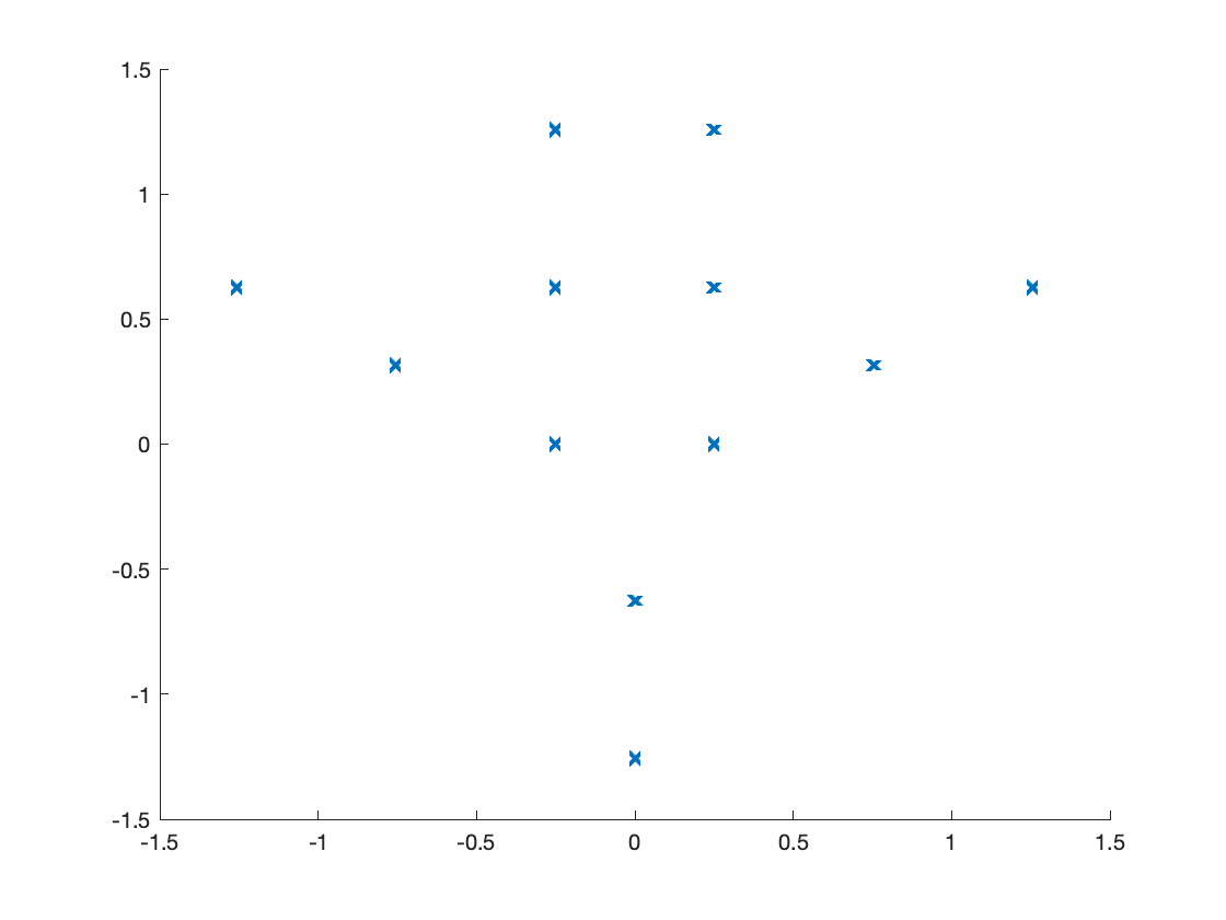
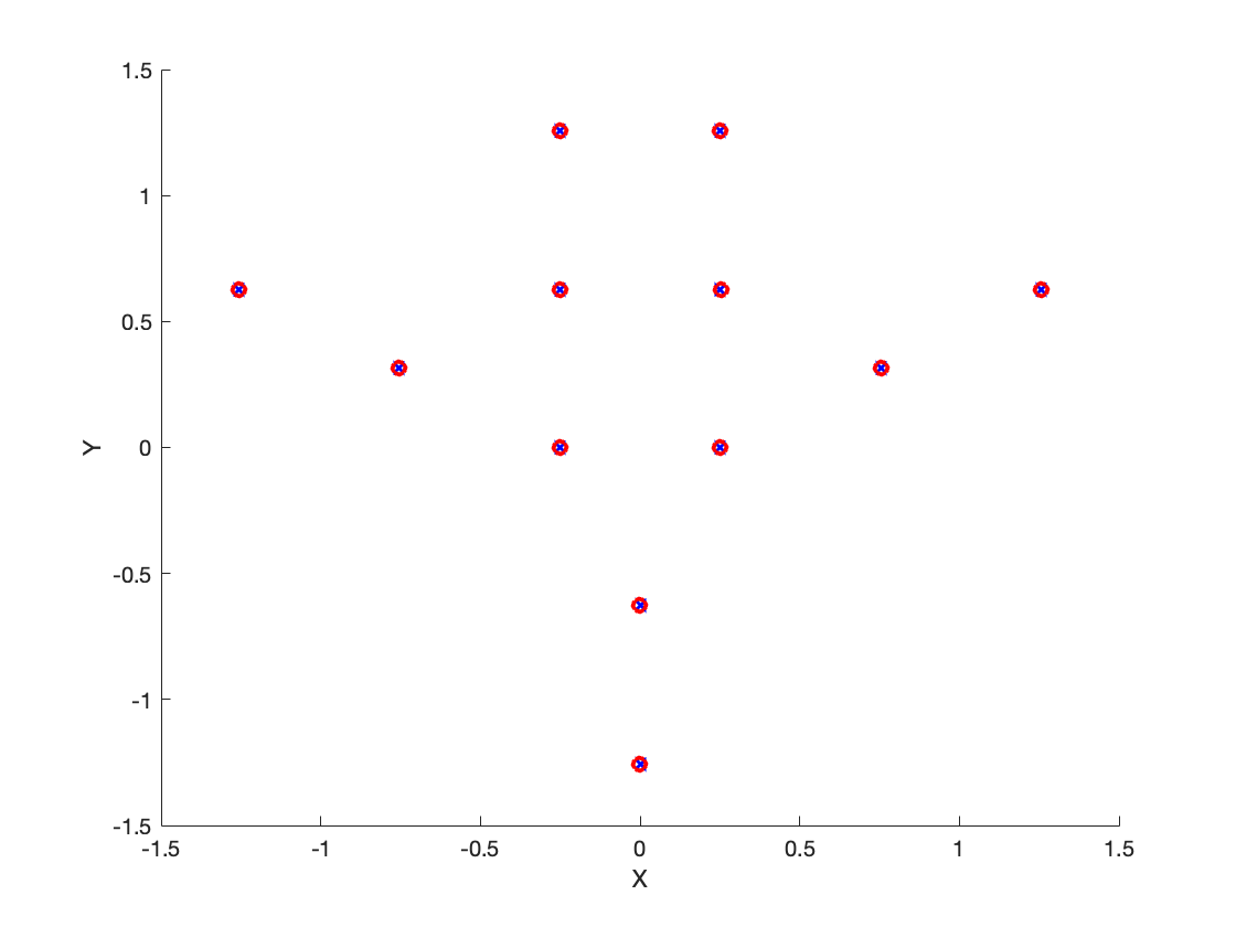
We will illustrate our algorithm by using an example of 2-d image which we obtain from [2], as shown in Figure 1. Following this paper, we take Δ1=(1.38,4.14)subscriptΔ11.384.14\Delta_{1}=(1.38,4.14), Δ2=(7.56,5.67)subscriptΔ27.565.67\Delta_{2}=(-7.56,5.67).

k𝑘k ωksubscript𝜔𝑘\omega_{k} aksubscript𝑎𝑘a_{k}
1 (1.2566,0.6283)1.25660.6283(-1.2566,0.6283) 50
2 (0.7540,0.3142)0.75400.3142(-0.7540,0.3142) 50
3 (0.2513,1.2566)0.25131.2566(-0.2513,1.2566) 50
4 (0.2513,0.6283)0.25130.6283(-0.2513,0.6283) 50
5 (0.2513,0)0.25130(-0.2513,0) 50
6 (0,0.6283)00.6283(0,-0.6283) 50
7 (0,1.2566)01.2566(0,-1.2566) 50
8 (0.2513,1.2566)0.25131.2566(0.2513,1.2566) 50
9 (0.2513,0.6283)0.25130.6283(0.2513,0.6283) 50
10 (0.2513,0)0.25130(0.2513,0) 50
11 (0.7540,0.3142)0.75400.3142(0.7540,0.3142) 50
12 (1.2566,0.6283)1.25660.6283(1.2566,0.6283) 50
Refer to caption
Figure 1: The two dimensional data comprising 12 points [2]. Left: The acutal points and amplitudes, Right: A graphic representation.

Let 𝐰1,,𝐰122subscript𝐰1subscript𝐰12superscript2\mathbf{w}_{1},\ldots,\mathbf{w}_{12}\in\mathbb{R}^{2} and {Δ1,Δ2}subscriptΔ1subscriptΔ2\{\Delta_{1},\Delta_{2}\} be a basis for 2superscript2\mathbb{R}^{2}. Here, we have

μ^(Δ2+Δ1)^𝜇subscriptΔ2subscriptΔ1\displaystyle\hat{\mu}(\Delta_{2}+\ell\Delta_{1}) =\displaystyle= k=112Akexp(iΔ2,𝐰k)exp(iΔ1,𝐰k)superscriptsubscript𝑘112subscript𝐴𝑘𝑖subscriptΔ2subscript𝐰𝑘𝑖subscriptΔ1subscript𝐰𝑘\displaystyle\sum_{k=1}^{12}A_{k}\exp(-i\langle\Delta_{2},\mathbf{w}_{k}\rangle)\exp(-i\ell\langle\Delta_{1},\mathbf{w}_{k}\rangle) (5.1)
μ^(Δ1+Δ2)^𝜇subscriptΔ1subscriptΔ2\displaystyle\hat{\mu}(\Delta_{1}+\ell\Delta_{2}) =\displaystyle= k=112Akexp(iΔ1,𝐰k)exp(iΔ2,𝐰k)superscriptsubscript𝑘112subscript𝐴𝑘𝑖subscriptΔ1subscript𝐰𝑘𝑖subscriptΔ2subscript𝐰𝑘\displaystyle\sum_{k=1}^{12}A_{k}\exp(-i\langle\Delta_{1},\mathbf{w}_{k}\rangle)\exp(-i\ell\langle\Delta_{2},\mathbf{w}_{k}\rangle) (5.2)

The number of samples required is 𝒪(qn)𝒪𝑞𝑛\mathcal{O}(qn), where q𝑞q is the dimension of the exponential sample, and n𝑛n is the degree of the localized kernel. We then apply our low pass filter and obtain

σn,1(x)subscript𝜎𝑛1𝑥\displaystyle\sigma_{n,1}(x) =\displaystyle= nk=112Akexp(iΔ2,𝐰k)Φn(xΔ1,𝐰k)subscriptPlanck-constant-over-2-pi𝑛superscriptsubscript𝑘112subscript𝐴𝑘𝑖subscriptΔ2subscript𝐰𝑘subscriptΦ𝑛𝑥subscriptΔ1subscript𝐰𝑘\displaystyle\hbar_{n}\sum_{k=1}^{12}A_{k}\exp(-i\langle\Delta_{2},\mathbf{w}_{k}\rangle)\Phi_{n}(x-\langle\Delta_{1},\mathbf{w}_{k}\rangle) (5.3)
σn,2(x)subscript𝜎𝑛2𝑥\displaystyle\sigma_{n,2}(x) =\displaystyle= nk=112Akexp(iΔ1,𝐰k)Φn(xΔ2,𝐰k)subscriptPlanck-constant-over-2-pi𝑛superscriptsubscript𝑘112subscript𝐴𝑘𝑖subscriptΔ1subscript𝐰𝑘subscriptΦ𝑛𝑥subscriptΔ2subscript𝐰𝑘\displaystyle\hbar_{n}\sum_{k=1}^{12}A_{k}\exp(-i\langle\Delta_{1},\mathbf{w}_{k}\rangle)\Phi_{n}(x-\langle\Delta_{2},\mathbf{w}_{k}\rangle) (5.4)

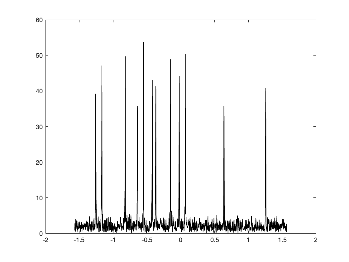
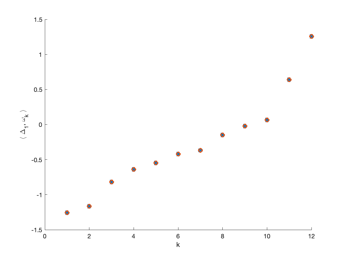
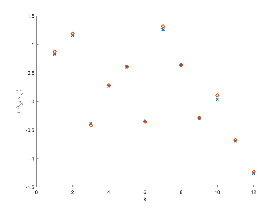
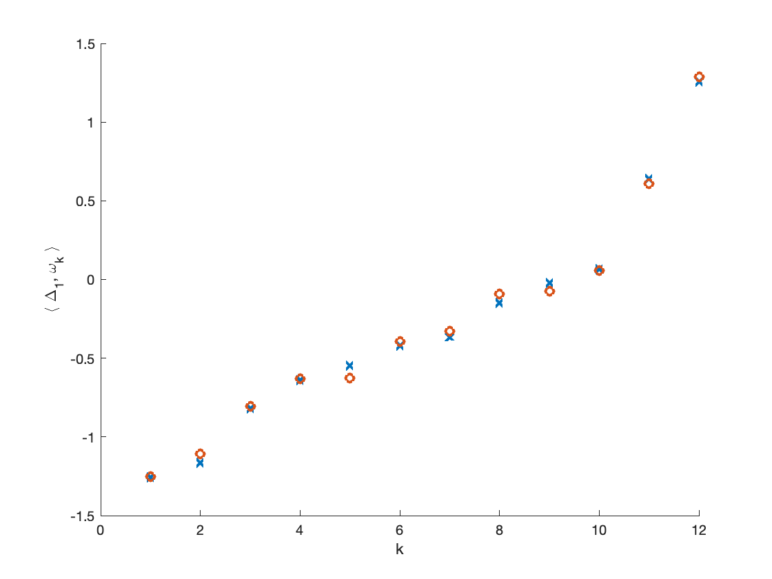
From the Theorem 4.1, Δ1,𝐰ksubscriptΔ1subscript𝐰𝑘\langle\Delta_{1},\mathbf{w}_{k}\rangle will be x𝑥x where the peaks occurs in |σn(x)|subscript𝜎𝑛𝑥|\sigma_{n}(x)|, Δ2,𝐰kPhase(σn(x))subscriptΔ2subscript𝐰𝑘𝑃𝑎𝑠𝑒subscript𝜎𝑛𝑥\langle\Delta_{2},\mathbf{w}_{k}\rangle\approx Phase\left(\sigma_{n}(x)\right), and Ak|σn(x)|subscript𝐴𝑘subscript𝜎𝑛𝑥A_{k}\approx|\sigma_{n}(x)|. Now, we can obtain the accurate estimation of Δ1,𝐰ksubscriptΔ1subscript𝐰𝑘\langle\Delta_{1},\mathbf{w}_{k}\rangle corresponding to less accurate estimation of Δ2,𝐰ksubscriptΔ2subscript𝐰𝑘\langle\Delta_{2},\mathbf{w}_{k}\rangle (Figure 2).

Refer to caption
Refer to caption
Refer to caption
Figure 2: Left: |σn,1(x)|subscript𝜎𝑛1𝑥|\sigma_{n,1}(x)|, middle: Accurate determination of Δ1,𝐰ksubscriptΔ1subscript𝐰𝑘\langle\Delta_{1},\mathbf{w}_{k}\rangle, right: Approximate estimation of Δ2,𝐰ksubscriptΔ2subscript𝐰𝑘\langle\Delta_{2},\mathbf{w}_{k}\rangle.

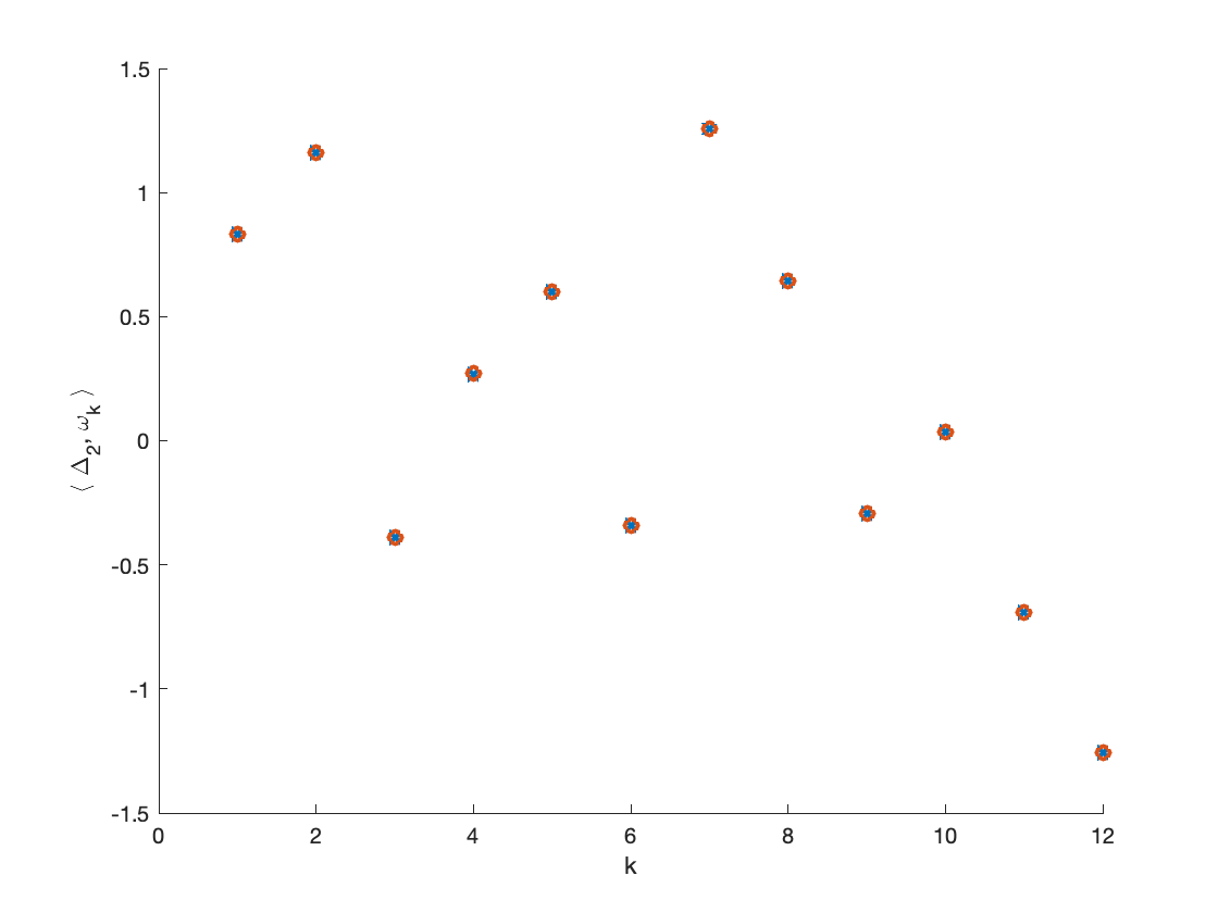
Then, we apply the same method in Δ2subscriptΔ2\Delta_{2} direction to obtain the accurate estimation of Δ2,𝐰ksubscriptΔ2subscript𝐰𝑘\langle\Delta_{2},\mathbf{w}_{k}\rangle corresponding to less accurate estimation of Δ1,𝐰ksubscriptΔ1subscript𝐰𝑘\langle\Delta_{1},\mathbf{w}_{k}\rangle (Figure 3 left and middle).

Finally, we can use nearest neighbor to obtain accurate estimation for both Δ1,𝐰ksubscriptΔ1subscript𝐰𝑘\langle\Delta_{1},\mathbf{w}_{k}\rangle corresponding to Δ2,𝐰ksubscriptΔ2subscript𝐰𝑘\langle\Delta_{2},\mathbf{w}_{k}\rangle and compute Aksubscript𝐴𝑘A_{k}. The final result is showed as the rightmost part of Figure 3.
Refer to caption
Refer to caption
Refer to caption
Figure 3: Left: Accurate estimation of Δ2,𝐰k.subscriptΔ2subscript𝐰𝑘\langle\Delta_{2},\mathbf{w}_{k}\rangle., Middle: approximate estimation of Δ2,𝐰k.subscriptΔ2subscript𝐰𝑘\langle\Delta_{2},\mathbf{w}_{k}\rangle., Right: Final reconstruction

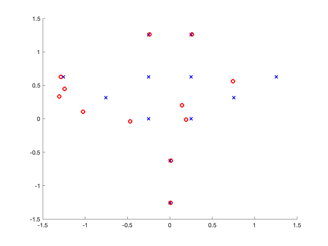
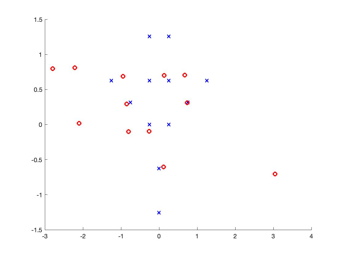
In comparison, we show the results obtained by MUSIC and ESPRIT algorithms in a graphic manner in Figure 4, and as a table in Table 1. It is obvious that both of these algorithms fail drastically even at high SNR levels.
Refer to caption
Refer to caption
Figure 4: The performance of (Left:) MUSIC and (Right:) ESPRIT algorithms on the 12 point 2 dimensional data set at SNR level of 60dB with 1024 samples.
Figure 5: ESPRIT approximation at 60dB.
SNR Method Total number of points Run-time Memory Accuracy RMSE Standard
(dB) Points reconstructed (seconds) (MB) (meters) (meters) Deviation
90 Localized 12 12 0.0045 0.42 0.3 0.0038 00
90 MUSIC 12 1 11.99 0.42 0.3 0.0376 0.00070.00070.0007
90 ESPRIT 12 12 0.0443 0.42 0.3 0.0279 0.01370.01370.0137
60 Localized 12 12 0.0045 0.42 0.3 0.0038 00
60 MUSIC 12 1 12.09 0.42 0.3 0.0378 0.00050.00050.0005
60 ESPRIT 12 8 0.04 0.42 0.3 0.0981 0.02500.02500.0250
30 Localized 12 12 0.0045 0.42 0.3 0.0038 00
30 MUSIC 12 1 10.96 0.42 0.3 0.0367 0.00580.00580.0058
30 ESPRIT 12 5 0.04 0.42 0.3 0.1355 0.05400.05400.0540
Table 1: The tables above compare results between our algorithm, MUSIC, and ESPRIT on 1024 number of samples.

5.3 Algorithm adaption in the three dimensional case

To extend our algorithm to 3-d problem, we can simply add another 3-d projection to our algorithm to find the points in the third coordinate that corresponding to the first and the second coordinates.

Let 𝐰1,,𝐰K3subscript𝐰1subscript𝐰𝐾superscript3\mathbf{w}_{1},\ldots,\mathbf{w}_{K}\in\mathbb{R}^{3} and {Δ1,Δ2,Δ3}subscriptΔ1subscriptΔ2subscriptΔ3\{\Delta_{1},\Delta_{2},\Delta_{3}\} be a basis for 3superscript3\mathbb{R}^{3}. Here, we have

μ^(Δ2+Δ1)^𝜇subscriptΔ2subscriptΔ1\displaystyle\hat{\mu}(\Delta_{2}+\ell\Delta_{1}) =\displaystyle= k=1KAkexp(iΔ2,𝐰k)exp(iΔ1,𝐰k)superscriptsubscript𝑘1𝐾subscript𝐴𝑘𝑖subscriptΔ2subscript𝐰𝑘𝑖subscriptΔ1subscript𝐰𝑘\displaystyle\sum_{k=1}^{K}A_{k}\exp(-i\langle\Delta_{2},\mathbf{w}_{k}\rangle)\exp(-i\ell\langle\Delta_{1},\mathbf{w}_{k}\rangle) (5.5)
μ^(Δ1+Δ2)^𝜇subscriptΔ1subscriptΔ2\displaystyle\hat{\mu}(\Delta_{1}+\ell\Delta_{2}) =\displaystyle= k=1KAkexp(iΔ1,𝐰k)exp(iΔ2,𝐰k)superscriptsubscript𝑘1𝐾subscript𝐴𝑘𝑖subscriptΔ1subscript𝐰𝑘𝑖subscriptΔ2subscript𝐰𝑘\displaystyle\sum_{k=1}^{K}A_{k}\exp(-i\langle\Delta_{1},\mathbf{w}_{k}\rangle)\exp(-i\ell\langle\Delta_{2},\mathbf{w}_{k}\rangle) (5.6)
μ^(Δ1+Δ3)^𝜇subscriptΔ1subscriptΔ3\displaystyle\hat{\mu}(\Delta_{1}+\ell\Delta_{3}) =\displaystyle= k=1KAkexp(iΔ1,𝐰k)exp(iΔ3,𝐰k)superscriptsubscript𝑘1𝐾subscript𝐴𝑘𝑖subscriptΔ1subscript𝐰𝑘𝑖subscriptΔ3subscript𝐰𝑘\displaystyle\sum_{k=1}^{K}A_{k}\exp(-i\langle\Delta_{1},\mathbf{w}_{k}\rangle)\exp(-i\ell\langle\Delta_{3},\mathbf{w}_{k}\rangle) (5.7)

By applying the low pass filter to the signals, we will get

σn,1(x)subscript𝜎𝑛1𝑥\displaystyle\sigma_{n,1}(x) =\displaystyle= nk=1KAkexp(iΔ2,𝐰k)Φn(xΔ1,𝐰k)subscriptPlanck-constant-over-2-pi𝑛superscriptsubscript𝑘1𝐾subscript𝐴𝑘𝑖subscriptΔ2subscript𝐰𝑘subscriptΦ𝑛𝑥subscriptΔ1subscript𝐰𝑘\displaystyle\hbar_{n}\sum_{k=1}^{K}A_{k}\exp(-i\langle\Delta_{2},\mathbf{w}_{k}\rangle)\Phi_{n}(x-\langle\Delta_{1},\mathbf{w}_{k}\rangle) (5.8)
σn,2(x)subscript𝜎𝑛2𝑥\displaystyle\sigma_{n,2}(x) =\displaystyle= nk=1KAkexp(iΔ1,𝐰k)Φn(xΔ2,𝐰k)subscriptPlanck-constant-over-2-pi𝑛superscriptsubscript𝑘1𝐾subscript𝐴𝑘𝑖subscriptΔ1subscript𝐰𝑘subscriptΦ𝑛𝑥subscriptΔ2subscript𝐰𝑘\displaystyle\hbar_{n}\sum_{k=1}^{K}A_{k}\exp(-i\langle\Delta_{1},\mathbf{w}_{k}\rangle)\Phi_{n}(x-\langle\Delta_{2},\mathbf{w}_{k}\rangle) (5.9)
σn,3(x)subscript𝜎𝑛3𝑥\displaystyle\sigma_{n,3}(x) =\displaystyle= nk=1KAkexp(iΔ1,𝐰k)Φn(xΔ3,𝐰k)subscriptPlanck-constant-over-2-pi𝑛superscriptsubscript𝑘1𝐾subscript𝐴𝑘𝑖subscriptΔ1subscript𝐰𝑘subscriptΦ𝑛𝑥subscriptΔ3subscript𝐰𝑘\displaystyle\hbar_{n}\sum_{k=1}^{K}A_{k}\exp(-i\langle\Delta_{1},\mathbf{w}_{k}\rangle)\Phi_{n}(x-\langle\Delta_{3},\mathbf{w}_{k}\rangle) (5.10)

From the Theorem 4.1, Δ1,𝐰ksubscriptΔ1subscript𝐰𝑘\langle\Delta_{1},\mathbf{w}_{k}\rangle will be x𝑥x where the peaks occurs in |σn(x)|subscript𝜎𝑛𝑥|\sigma_{n}(x)|, Δ2,𝐰kPhase(σn(x))subscriptΔ2subscript𝐰𝑘𝑃𝑎𝑠𝑒subscript𝜎𝑛𝑥\langle\Delta_{2},\mathbf{w}_{k}\rangle\approx Phase\left(\sigma_{n}(x)\right), and Ak|σn(x)|subscript𝐴𝑘subscript𝜎𝑛𝑥A_{k}\approx|\sigma_{n}(x)|. Now, we can obtain the accurate estimation of Δ1,𝐰ksubscriptΔ1subscript𝐰𝑘\langle\Delta_{1},\mathbf{w}_{k}\rangle corresponding to less accurate estimation of Δ2,𝐰ksubscriptΔ2subscript𝐰𝑘\langle\Delta_{2},\mathbf{w}_{k}\rangle.

Then, we apply the same method in Δ2subscriptΔ2\Delta_{2} and Δ3subscriptΔ3\Delta_{3} directions to obtain the accurate estimation of Δ2,𝐰ksubscriptΔ2subscript𝐰𝑘\langle\Delta_{2},\mathbf{w}_{k}\rangle and Δ3,𝐰ksubscriptΔ3subscript𝐰𝑘\langle\Delta_{3},\mathbf{w}_{k}\rangle corresponding to less accurate estimation of Δ1,𝐰ksubscriptΔ1subscript𝐰𝑘\langle\Delta_{1},\mathbf{w}_{k}\rangle respectively.

Finally, we can use nearest neighbor to obtain accurate estimation for all Δ1,𝐰ksubscriptΔ1subscript𝐰𝑘\langle\Delta_{1},\mathbf{w}_{k}\rangle, Δ2,𝐰ksubscriptΔ2subscript𝐰𝑘\langle\Delta_{2},\mathbf{w}_{k}\rangle, Δ3,𝐰ksubscriptΔ3subscript𝐰𝑘\langle\Delta_{3},\mathbf{w}_{k}\rangle and compute Ak=|σn(x)|subscript𝐴𝑘subscript𝜎𝑛𝑥A_{k}=|\sigma_{n}(x)|.

5.4 Results in three dimensional experiments

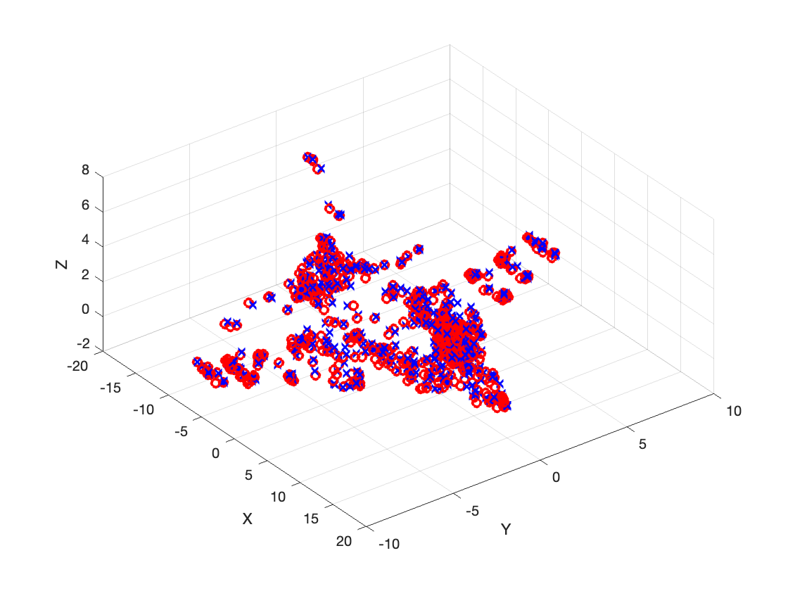
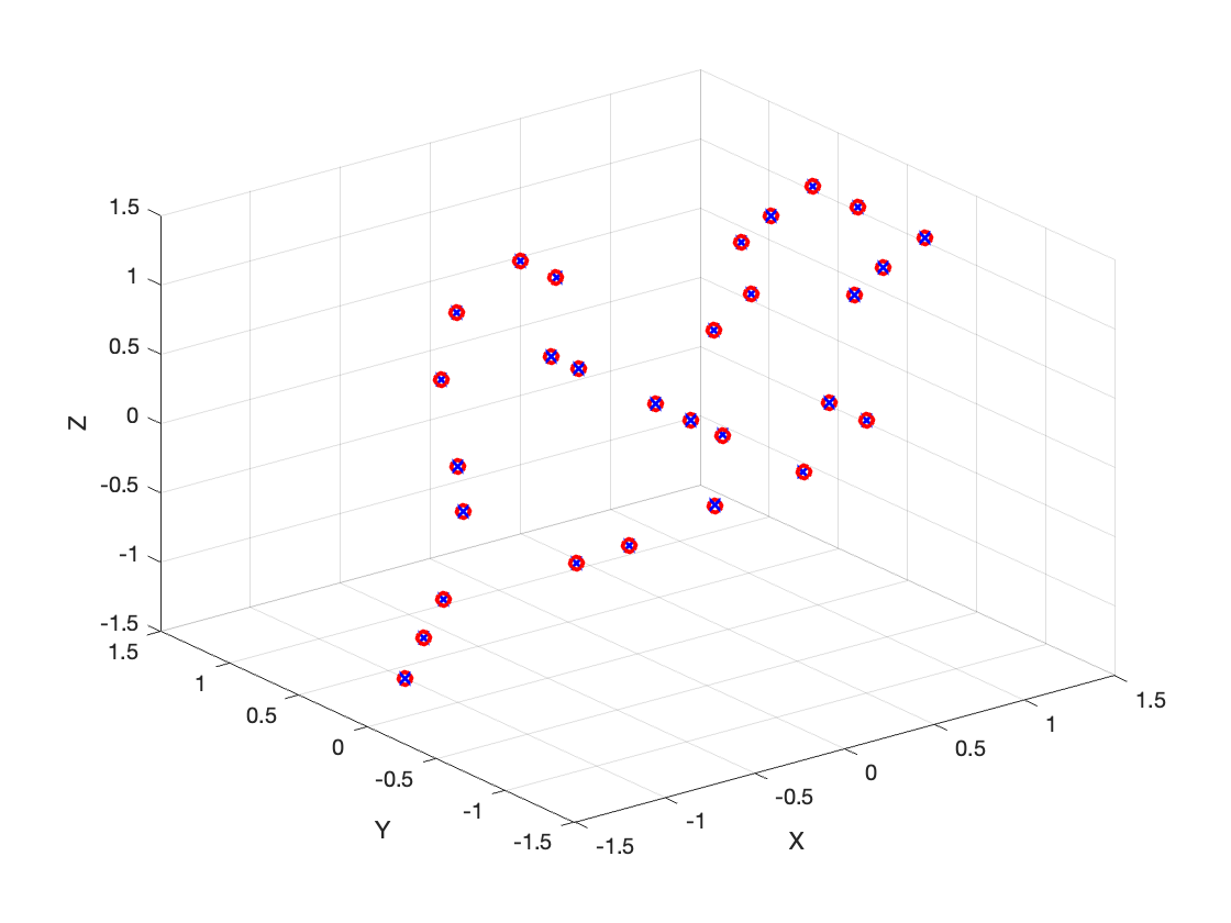
We tested our method described in Section 5.3 on two three dimensional data sets as described in [2], one comprising 29 points and the other comprising 1000 points. Figure 6 shows the results in a special case in a graphical manner.
Refer to caption
Refer to caption
Figure 6: Left: Recuperation of 29 points with 65536 samples at -10dB noise level, Right: Recuperation of 1000 points with 65536 samples at 5dB noise level.

Our algorithm is able to reconstruct all 29 points of 3-d tomographic image accurately as shown in figure 6. The samples required by our method are 65,536 samples with -10 dB noise added to the data. As comparison to the original paper [2], the author required 42,875 samples to reconstruct all 29 points with noise levels varying from 40 dB SNR to 5 dB SNR.

In the 1000 points of 3-d fighter jet image, our algorithm cannot separate the signals that are really close together due to high density data points on a cluster. We can only reconstruct 903 data points of out 1000 points with 655366553665536 samples. This method requires approximately 35MB of memory and the run-time is less than 1 second. Comparing to our baseline result from [2], the author has experimented with 72000, 90000, and 180000 samples with the result of 71% of the scatterers is reconstructed within an error of at most 10 cm and 93% within 30 cm, 81% within 10 cm and 95% within 30 cm, 94% within 10 cm and 98% within 30 cm respectively. One may see that the advantage of our algorithm in terms of speed and accuracy.

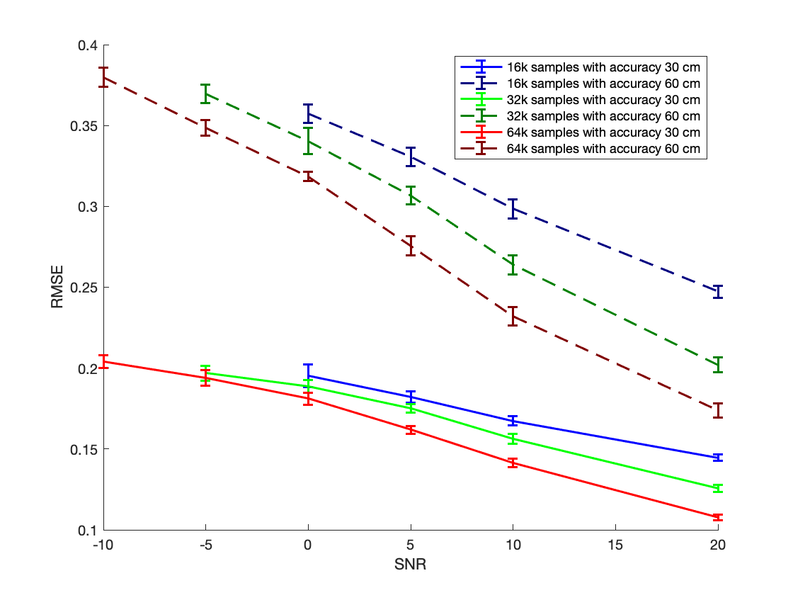
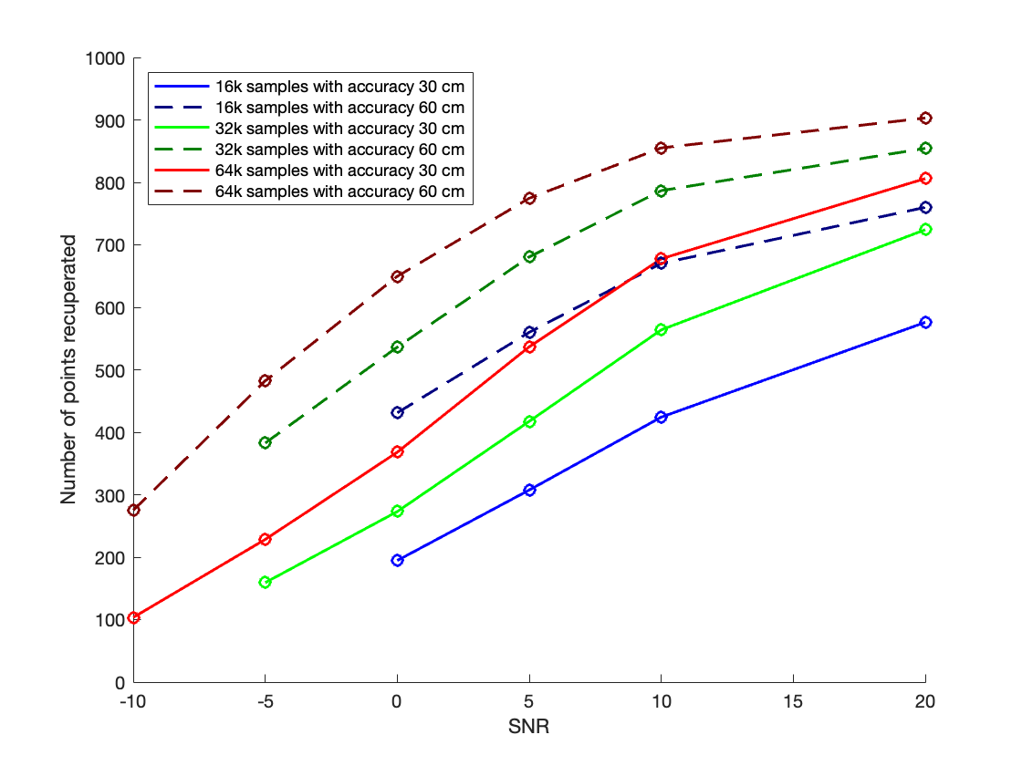
Figure 7 shows the dependence on the SNR of the accuracy and the number of points recuperated out of the 1000 points.
Refer to caption
Refer to caption
Figure 7: For the 1000 point data set, dependence on SNR for (Left:) accuracy and (Right:) number of points recuperated.

Finally, the details of all the results are summarized in Table 2.

SNR Number of Total number of points Run-time Memory Accuracy RMSE Standard
(dB) samples Points reconstructed (seconds) (MB) (meters) (meters) Deviation
-10 8192 12 12 0.04 2.58 0.3 0.0003 1.09×1051.09superscript1051.09\times 10^{-5}
-10 65536 29 29 0.36 20.53 0.3 0.0007 0.00030.00030.0003
20 16384 1000 575 0.63 14.88 0.3 0.1445 0.00200.00200.0020
10 16384 1000 424 0.75 14.68 0.3 0.1673 0.00290.00290.0029
5 16384 1000 307 0.67 14.52 0.3 0.1819 0.00350.00350.0035
0 16384 1000 194 0.95 14.44 0.3 0.1952 0.00680.00680.0068
20 16384 1000 760 0.62 14.85 0.6 0.2473 0.00370.00370.0037
10 16384 1000 670 0.87 14.81 0.6 0.2984 0.00600.00600.0060
5 16384 1000 559 0.69 14.58 0.6 0.3305 0.00540.00540.0054
0 16384 1000 431 0.87 14.45 0.6 0.3572 0.00550.00550.0055
20 32768 1000 724 0.52 21.97 0.3 0.1256 0.00230.00230.0023
10 32768 1000 563 0.81 21.82 0.3 0.1561 0.00300.00300.0030
5 32768 1000 417 1.06 21.78 0.3 0.1752 0.00260.00260.0026
0 32768 1000 273 1.31 21.57 0.3 0.1886 0.00390.00390.0039
-5 32768 1000 159 1.50 21.20 0.3 0.1969 0.00450.00450.0045
20 32768 1000 854 0.64 21.99 0.6 0.2020 0.00450.00450.0045
10 32768 1000 786 0.75 21.95 0.6 0.2638 0.00570.00570.0057
5 32768 1000 680 1.04 21.91 0.6 0.3067 0.00520.00520.0052
0 32768 1000 536 1.26 21.77 0.6 0.3404 0.00800.00800.0080
-5 32768 1000 382 1.75 21.46 0.6 0.3695 0.00570.00570.0057
20 65536 1000 806 0.58 35.64 0.3 0.1077 0.00180.00180.0018
10 65536 1000 677 0.68 35.59 0.3 0.1413 0.00250.00250.0025
5 65536 1000 536 0.90 35.49 0.3 0.1618 0.00250.00250.0025
0 65536 1000 367 1.24 35.34 0.3 0.1810 0.00370.00370.0037
-5 65536 1000 228 1.95 35.20 0.3 0.1939 0.00480.00480.0048
-10 65536 1000 103 7.33 35.71 0.3 0.2040 0.00400.00400.0040
20 65536 1000 903 0.56 35.62 0.6 0.1736 0.00430.00430.0043
10 65536 1000 855 0.74 35.61 0.6 0.2320 0.00570.00570.0057
5 65536 1000 774 0.83 35.56 0.6 0.2755 0.00600.00600.0060
0 65536 1000 649 1.34 35.50 0.6 0.3185 0.00300.00300.0030
-5 65536 1000 482 2.07 35.26 0.6 0.3485 0.00470.00470.0047
-10 65536 1000 275 7.07 35.25 0.6 0.3798 0.00580.00580.0058
Table 2: The tables above show full performances of our algorithm.

6 Conclusions

The problem of multidimensional exponential analysis arises in many areas of applications including tomographic imaging, ISAR imaging, antenna array processing, etc. The problem is essentially to develop an efficient algorithm to obtain the inverse Fourier transform of a multidimensional signal, based on finitely many equidistant samples of the signal. We have given a very simple algorithm based on localized trigonometric kernel, which reduces the problem to a series of one dimensional problems. Our algorithm works with a tractable number of samples, gives high accuracy, and is very robust even in the presence of noise as high as -10dB. We have proved theoretical guarantees under the assumption that the noise is sub-Gaussian, a significantly weaker assumption that the assumption of white noise common in the literature.

References

  • [1] Stéphane Boucheron, Gábor Lugosi, and Pascal Massart. Concentration inequalities: A nonasymptotic theory of independence. Oxford university press, 2013.
  • [2] Annie Cuyt, Yuan Hou, Ferre Knaepkens, and Wen-shin Lee. Sparse multidimensional exponential analysis with an application to radar imaging. SIAM Journal on Scientific Computing, 42(3):B675–B695, 2020.
  • [3] Annie Cuyt and Wen-shin Lee. Multivariate exponential analysis from the minimal number of samples. Advances in Computational Mathematics, 44:987–1002, 2018.
  • [4] Benedikt Diederichs. Sparse frequency estimation: Stability and algorithms. PhD thesis, Staats-und Universitätsbibliothek Hamburg Carl von Ossietzky, 2018.
  • [5] Benedikt Diederichs, Mihail N Kolountzakis, and Effie Papageorgiou. How many fourier coefficients are needed? Monatshefte für Mathematik, 200(1):23–42, 2023.
  • [6] F. Filbir, H. N. Mhaskar, and J Prestin. On the problem of parameter estimation in exponential sums. Constructive Approximation, 35(3):323–343, 2012.
  • [7] H. Krim and M. Viberg. Two decades of array signal processing research: the parametric approach. Signal Processing Magazine, IEEE, 13(4):67–94, 1996.
  • [8] Stefan Kunis, Thomas Peter, Tim Römer, and Ulrich von der Ohe. A multivariate generalization of prony’s method. Linear Algebra and its Applications, 490:31–47, 2016.
  • [9] H. N. Mhaskar and J. Prestin. On local smoothness classes of periodic functions. Journal of Fourier Analysis and Applications, 11(3):353–373, 2005.
  • [10] Frank WJ Olver. Asymptotics and special functions. Academic press, 2014.
  • [11] Thomas Peter, Gerlind Plonka, and Robert Schaback. Prony’s method for multivariate signals. Pamm, 15(1):665–666, 2015.
  • [12] D. Potts and M. Tasche. Parameter estimation for exponential sums by approximate Prony method. Signal Processing, 90(5):1631–1642, 2010.
  • [13] Daniel Potts and Manfred Tasche. Parameter estimation for multivariate exponential sums. Electron. Trans. Numer. Anal, 40(204-224):94, 2013.
  • [14] André Quinquis, Emanuel Radoi, and F-C Totir. Some radar imagery results using superresolution techniques. IEEE Transactions on Antennas and Propagation, 52(5):1230–1244, 2004.
  • [15] Ramachandran S Raghavan. A generalized version of ace and performance analysis. IEEE Transactions on Signal Processing, 68:2574–2585, 2020.
  • [16] Souleymen Sahnoun, Konstantin Usevich, and Pierre Comon. Multidimensional esprit for damped and undamped signals: Algorithm, computations, and perturbation analysis. IEEE Transactions on Signal Processing, 65(22):5897–5910, 2017.
  • [17] Tomas Sauer. Prony’s method in several variables: symbolic solutions by universal interpolation. Journal of Symbolic Computation, 84:95–112, 2018.
  • [18] James Alexander Shohat and Jacob David Tamarkin. The problem of moments, volume 1. American Mathematical Society (RI), 1950.
  • [19] Shyam Venkatasubramanian, Sandeep Gogineni, Bosung Kang, Ali Pezeshki, Muralidhar Rangaswamy, and Vahid Tarokh. Toward data-driven radar stap. arXiv preprint arXiv:2209.02890, 2022.
  • [20] Zhihui Zhu, Gongguo Tang, Pawan Setlur, Sandeep Gogineni, Michael B Wakin, and Muralidhar Rangaswamy. Super-resolution in sar imaging: Analysis with the atomic norm. In 2016 IEEE Sensor Array and Multichannel Signal Processing Workshop (SAM), pages 1–5. IEEE, 2016.