Iterated Invariant Extended Kalman Filter (IIEKF)

Abstract

In this paper, we introduce the Iterated Invariant Extended Kalman Filter (IIEKF), which is an invariant extended Kalman filter (IEKF) where the updated state in the light of the latest measurement is defined as a maximum a posteriori (MAP) estimate. Under some compatibility requirements on the output map, we prove strong mathematical guarantees which echo those of the Kalman filter in the linear case. We apply the technique to two problems: solving a system of equations on a Lie group, and a problem of engineering interest, namely ego-localization of the hook of a crane. The latter serves as a benchmarking example, where the IIEKF favorably compares to other filters.

1 Introduction

The Kalman filter [1] solves in any respect the problem of estimating the state of a linear dynamical system from linear measurements corrupted by Gaussian noises. To accommodate nonlinearity of physical models and measurements, the Extended Kalman Filter (EKF), early developed in the Apollo program, and still very lively, relies on linearizations. However, linearization errors were soon recognized to degrade performance [2]. This motivated the development of iterative filtering algorithms such as the iterated EKF [3, 4, 5], iterated EKF on Lie groups [6, 7], and smoothers [8], where the discrepancy between the nonlinear output function and its first-order approximation is reduced by refining the operating point. It also inspired other iterative algorithms, such as the iterated extended Kalman particle filter [9].

On another note, the EKF, as an extension of the linear Kalman filter, inherently uses the vector space structure of the state space, and ignores all geometric properties the problem may possess. This latter concern has led to the development of geometric filtering methods, which today constitute a field of study in their own right. As concerns observer design, geometric methods may be traced back to attitude and pose estimation [10, 11, 12]. When turning to the more general problem of inertial navigation and localization, the invariant extended Kalman filter (IEKF) [13, 14] has become a key alternative to the standard EKF. Its theoretical properties include convergence guarantees [13], consistency properties for Simultaneous Localization and Mapping (SLAM) in robotics [14], see also related works [15, 16, 17], and have led to applications in various fields, [14, 8, 18, 19, 20, 21, 15] and in the industry [14]. The field of observers has benefited from the introduction of new groups brought by the IEKF theory, see e.g., [22, 23, 24], namely the groups $SE_{2}(3)$ and $SE_{k}(d)$ introduced in [25, 13] and their relation to the navigation equations. A unifying perspective on the Lie groups that arise from the IEKF theory can be found in the recent paper [26]. The vibrant equivariant observer framework, see [27], is closely related.

In this paper, we introduce the iterated invariant extended Kalman filter (IIEKF). The rationale is to focus on the measurement update step of the invariant extended Kalman filter (IEKF) [14] and to improve it using the Gauss-Newton (GN) method [28]. Instead of attempting to explicitly account for the manifold structure of the state space to adapt the optimization algorithm of the iterated EKF at a general level as in [6], we make a limited number of modifications to the IEKF, by seeking the updated state as the maximum a posteriori (MAP) in terms of the linearized invariant error in the Lie algebra. We start by first explicitating the sensible properties of the linear Kalman filter we seek to elicit in a nonlinear context, and then we prove the IIEKF possesses them indeed. The differences between the proposed method and the general iterated EKF on Lie groups from [6] and [7] are detailed in Appendix D.

The fact the IIEKF recovers a number of provable properties and guarantees of the linear case, although in a nonlinear context, is made possible by the fact we consider specific state spaces (Lie groups), and specific output maps, namely the invariant measurements of [13]. To come up with mathematical properties, we consider the limit case where the measurement noise goes to zero. This limit case is particularly meaningful, as the improvements brought by iterative methods are sharper when measurements are accurate, since refining the linearization point then pays off greatly.

The method is applied to two different problems. The first problem is the analog to the mathematical problem of solving a system of linear equations, but when the unknown lives in a Lie group. The second problem, is a problem of engineering interest, that allows for comparisons between the proposed IIEKF, the IEKF, the EKF, and the iterated EKF.

Throughout the paper, the acronym IEKF is reserved for the invariant EKF, whereas we use IterEKF for the iterated EKF.

The paper is structured as follows. Section 2 recalls the equations of the Kalman filter, EKF, and iterated EKF. Section 3 analyzes the update step of the KF and EKF in the case of noise-free measurements. The desirable properties we expect from a probabilistic filter in the noise-free measurement case are then developed. Section 4 introduces the proposed IIEKF algorithm for both noisy and noise-free measurements. Section 5 presents the theoretical properties of the IIEKF. Section 6 applies the method to the problem of solving a system of equations on a Lie group. A simple example on $SO(3)$ sheds light on the way the IIEKF operates. Finally, Section 7 compares the performance of the proposed algorithm and other state-of-the-art filters on the problem of estimating the extended pose (orientation, velocity, position) of the hook of a crane on which an inertial measurement unit (IMU) is mounted.

2 Kalman filter, EKF, iterated EKF

The goal of the present section is to fix notation and summarize a few known facts.

2.1 Kalman filter equations

Consider the linear system

$$\mathbf{x}_{k+1} =\mathbf{F}_{k}\mathbf{x}_{k}+\mathbf{B}_{k}\mathbf{u}_{k}+\mathbf{w}_{k},$$ (1a)

$$\mathbf{y}_{k} =\mathbf{H}_{k}\mathbf{x}_{k}+\mathbf{n}_{k},$$ (1b)

where $\mathbf{x}_{k}\in\mathbb{R}^{n}$, $\mathbf{y}_{k}\in\mathbb{R}^{m}$, $\mathbf{u}_{k}\in\mathbb{R}^{b}$, $\mathbf{F}_{k}\in\mathbb{R}^{n\times n}$, $\mathbf{B}_{k}\in\mathbb{R}^{n\times b}$, and $\mathbf{H}_{k}\in\mathbb{R}^{m\times n}$. The process and measurement noises are such that $\mathbf{w}_{k}\sim\mathcal{N}(\mathbf{0},\mathbf{Q}_{k})$ and $\mathbf{n}_{k}\sim\mathcal{N}(\mathbf{0},\mathbf{N}_{k})$.

The Kalman filter (KF) computes at all times the statistics of the state $\mathbf{x}_{k}$ given the measurements gathered so far.

Propagation

At propagation step, the KF computes

$$\hat{\mathbf{x}}_{k+1} =\mathbf{F}_{k}\hat{\mathbf{x}}_{k}+\mathbf{B}_{k}\mathbf{u}_{k},$$ (2a)

$$\mathbf{P}_{k+1} =\mathbf{F}_{k}\mathbf{P}_{k}\mathbf{F}_{k}^{T}+\mathbf{Q}_{k}.$$ (2b)

Assuming $p(\mathbf{x}_{k}\mid\mathbf{y}_{0},\ldots,\mathbf{y}_{k})=\mathcal{N}(\hat{\mathbf{x}}_{k},\mathbf{P}_{k})$, we have that (2) ensures $p(\mathbf{x}_{k+1}\mid\mathbf{y}_{0},\ldots,\mathbf{y}_{k})=\mathcal{N}(\hat{\mathbf{x}}_{k+1},\mathbf{P}_{k+1})$.

Update

Departing from $p(\mathbf{x}_{k}\mid\mathbf{y}_{0},\ldots,\mathbf{y}_{k-1})=\mathcal{N}(\hat{\mathbf{x}}_{k},\mathbf{P}_{k})$, and receiving measurement $\mathbf{y}_{k}$ from (1b), the KF updates the estimates according to the equations

$$\mathbf{z}_{k} =\mathbf{y}_{k}-\mathbf{H}_{k}\hat{\mathbf{x}}_{k},$$ (3a)

$$\mathbf{S}_{k} =\mathbf{H}_{k}\mathbf{P}_{k}\mathbf{H}_{k}^{T}+\mathbf{N}_{k},$$ (3b)

$$\mathbf{K}_{k} =\mathbf{P}_{k}\mathbf{H}_{k}^{T}\mathbf{S}_{k}^{-1},$$ (3c)

$$\hat{\mathbf{x}}^{+}_{k} =\hat{\mathbf{x}}_{k}+\mathbf{K}_{k}\mathbf{z}_{k},$$ (3d)

$$\mathbf{P}^{+}_{k} =(\mathbf{I}-\mathbf{K}_{k}\mathbf{H}_{k})\mathbf{P}_{k},$$ (3e)

where $\mathbf{z}_{k}$ is the innovation (i.e., a prediction error), $\mathbf{S}_{k}$ is the innovation covariance, and $\mathbf{K}_{k}$ is the Kalman gain. We have then $p(\mathbf{x}_{k}\mid\mathbf{y}_{0},\ldots,\mathbf{y}_{k})=\mathcal{N}(\hat{\mathbf{x}}_{k}^{+},\mathbf{P}_{k}^{+})$.

2.2 Extended Kalman filter equations

Consider now the nonlinear system

$$\mathbf{x}_{k+1} =\mathbf{f}(\mathbf{x}_{k},\mathbf{u}_{k},\mathbf{w}_{k}),$$ (4a)

$$\mathbf{y}_{k} =\mathbf{h}_{k}(\mathbf{x}_{k})+\mathbf{n}_{k},$$ (4b)

where $\mathbf{f}$ and $\mathbf{h}_{k}$ are nonlinear functions. Owing to nonlinearity, the extended Kalman filter (EKF) maintains a Gaussian approximation, called “belief”, of the (intractable) statistics of the state $\mathbf{x}_{k}$, given the measurements gathered so far.

Propagation

The EKF propagates its belief through the state dynamics model as

$$\hat{\mathbf{x}}_{k+1} =\mathbf{f}(\hat{\mathbf{x}}_{k},\mathbf{u}_{k},\mathbf{0}),$$ (5a)

$$\mathbf{P}_{k+1} =\mathbf{F}_{k}\mathbf{P}_{k}\mathbf{F}_{k}^{T}+\mathbf{G}_{k}\mathbf{Q}_{k}\mathbf{G}_{k}^{T},$$ (5b)

where $\mathbf{F}_{k}$ and $\mathbf{G}_{k}$ are the Jacobians of $\mathbf{f}$ with respect to (w.r.t.) $\mathbf{x}_{k}$ and $\mathbf{w}_{k}$ respectively, evaluated at $(\hat{\mathbf{x}}_{k},\mathbf{u}_{k},\mathbf{0})$.

Update

The EKF linearizes the function $\mathbf{h}_{k}$ around the current estimate $\hat{\mathbf{x}}_{k}$, yielding Jacobian $\mathbf{H}_{k}$. It uses the same update equations as the KF, except for the innovation that now writes $\mathbf{z}_{k}=\mathbf{y}_{k}-\mathbf{h}_{k}(\hat{\mathbf{x}}_{k})$.

2.3 Updated state and the maximum a posteriori (MAP)

Consider again measurement (4b) given by

$$\mathbf{y}_{k}=\mathbf{h}_{k}(\mathbf{x}_{k})+\mathbf{n}_{k}.$$ (6)

Let us start from a prior Gaussian belief $p(\mathbf{x}_{k}\mid\mathbf{y}_{0},\ldots,\mathbf{y}_{k-1}):=\tilde{p}(\mathbf{x}_{k})$ in the form of a Gaussian $\mathcal{N}(\hat{\mathbf{x}}_{k},\mathbf{P}_{k})$. In the light of a present measurement $\mathbf{y}_{k}$ the maximum a posteriori (MAP) estimate is obtained by minimizing the posterior negative log likelihood, i.e.,

$$\hat{\mathbf{x}}_{k}^{\star} =\operatorname*{argmin}_{\mathbf{x}}-\ln(\tilde{p}(\mathbf{x}\mid\mathbf{y}_{k})),$$ (7a)

$$=\operatorname*{argmin}_{\mathbf{x}}-\ln\left(p(\mathbf{y}_{k}\mid\mathbf{x})\tilde{p}(\mathbf{x})\right)+\mathrm{constant},$$ (7b)

$$=\operatorname*{argmin}_{\mathbf{x}}\frac{1}{2}\|\mathbf{x}-\hat{\mathbf{x}}_{k}\|^{2}_{\mathbf{P}_{k}}+\frac{1}{2}\|\mathbf{y}_{k}-\mathbf{h}_{k}(\mathbf{x})\|^{2}_{\mathbf{N}_{k}},$$ (7c)

where we used the Bayes rule and $\|\mathbf{x}\|^{2}_{\mathbf{P}}=\mathbf{x}^{T}\mathbf{P}^{-1}\mathbf{x}$ denotes the squared Mahalanobis distance.

In the case where $\mathbf{h}_{k}$ is linear, i.e., $\mathbf{y}_{k}=\mathbf{H}_{k}\mathbf{x}_{k}+\mathbf{n}_{k}$, the estimate $\hat{\mathbf{x}}_{k}^{+}$ provided by (3d) exactly solves the optimization problem (7c). However, when $\mathbf{h}_{k}$ is a nonlinear function, the estimate provided by the EKF is the result of a linearization and is only an approximation to the solution of problem (7c).

2.4 The iterated EKF

The optimization problem of finding the MAP may be addressed through the Gauss-Newton method, leading to the iterated EKF, as shown by [3].

Lemma 1 (from [3]).

Consider the optimization problem

$$\mathbf{x}^{\star}=\operatorname*{argmin}_{\mathbf{x}}\frac{1}{2}\|\mathbf{x}-\bar{\mathbf{x}}\|^{2}_{\mathbf{A}}+\frac{1}{2}\|\mathbf{b}-\bar{\mathbf{h}}(\mathbf{x})\|^{2}_{\mathbf{B}},$$ (8)

with $\mathbf{x},\bar{\mathbf{x}}\in\mathbb{R}^{n}$, $\mathbf{b}\in\mathbb{R}^{m}$, $\mathbf{A}\in\mathbb{R}^{n\times n}$, $\mathbf{B}\in\mathbb{R}^{m\times m}$ and $\bar{\mathbf{h}}:\mathbb{R}^{n}\rightarrow\mathbb{R}^{m}$. This problem can be attacked with the Gauss-Newton (GN) method, yielding the sequence of estimates

$$\mathbf{x}^{i+1}=\bar{\mathbf{x}}+\bar{\mathbf{K}}^{i}(\mathbf{b}-\bar{\mathbf{h}}(\mathbf{x}^{i})-\bar{\mathbf{H}}^{i}(\bar{\mathbf{x}}-\mathbf{x}^{i})),$$ (9)

with

$$\bar{\mathbf{H}}^{i} =\bar{\mathbf{h}}^{\prime}(\mathbf{x}^{i}),$$ (10a)

$$\bar{\mathbf{K}}^{i} =\mathbf{A}(\bar{\mathbf{H}}^{i})^{T}(\bar{\mathbf{H}}^{i}\mathbf{A}(\bar{\mathbf{H}}^{i})^{T}+\mathbf{B})^{-1},$$ (10b)

where $\bar{\mathbf{h}}^{\prime}(\mathbf{x}^{i})$ denotes the Jacobian of $\bar{\mathbf{h}}$ evaluated at $\mathbf{x}^{i}$.

One may bring Lemma 1 to bear on the optimization problem (7c) of finding the most likely estimate in the light of latest measurement. It leads to the equations of the iterated EKF (IterEKF), see [3], that is,

$$\hat{\mathbf{x}}_{k}^{i+1} =\hat{\mathbf{x}}_{k}+\mathbf{K}_{k}^{i}(\mathbf{y}_{k}-\mathbf{h}_{k}(\mathbf{x}_{k}^{i})-\mathbf{H}_{k}^{i}(\hat{\mathbf{x}}_{k}-\mathbf{x}_{k}^{i})),$$ (11a)

$$\mathbf{H}_{k}^{i} =\mathbf{h}_{k}^{\prime}(\mathbf{x}_{k}^{i}),$$ (11b)

$$\mathbf{K}_{k}^{i} =\mathbf{P}_{k}(\mathbf{H}_{k}^{i})^{T}(\mathbf{H}_{k}^{i}\mathbf{P}_{k}(\mathbf{H}_{k}^{i})^{T}+\mathbf{N}_{k})^{-1}.$$ (11c)

Since we initialize at $\mathbf{x}_{k}^{0}=\hat{\mathbf{x}}_{k}$, we note the conventional EKF then amounts to one Gauss-Newton iteration.

3 Desirable properties to expect in the face of noise-free measurements

In this section, we inspect the case where measurement noise tends to zero. This allows us to set the stage for the problems we will solve.

3.1 Noise-free measurements

As sensors get more accurate, the eigenvalues $\lambda_{j}(\mathbf{N}_{k})$ of covariance matrix $\mathbf{N}_{k}$ get smaller and smaller. In the limit case of noise-free measurements, i.e., $\lambda_{j}(\mathbf{N}_{k})=0$ for all $j$, the unconstrained optimization problem (7c) becomes the following constrained optimization problem, see [29],

$$\hat{\mathbf{x}}_{k}^{\star}=\operatorname*{argmin}\limits_{\mathbf{x}}\left\{\frac{1}{2}\|\mathbf{x}-\hat{\mathbf{x}}_{k}\|^{2}_{\mathbf{P}_{k}}\mid\mathbf{h}_{k}(\mathbf{x})=\mathbf{y}_{k}\right\}.$$ (12)

Let us focus on the linear case, and set $\mathbf{N}_{k}=\mathbf{0}$. The KF update then becomes

$$\hat{\mathbf{x}}_{k}^{+}=\hat{\mathbf{x}}_{k}+\underbrace{\mathbf{P}_{k}\mathbf{H}_{k}^{T}(\mathbf{H}_{k}\mathbf{P}_{k}\mathbf{H}_{k}^{T})^{-1}}_{\mathbf{K}_{k}}\underbrace{(\mathbf{y}_{k}-\mathbf{h}_{k}(\hat{\mathbf{x}}_{k}))}_{\mathbf{z}_{k}}.$$ (13)

Provided that $\mathbf{H}_{k}\mathbf{P}_{k}\mathbf{H}_{k}^{T}$ is invertible, it returns the solution of the constrained optimization problem.

Noise-free measurements, which will play an important role in the sequel, completely remove uncertainty in the observed directions. This brings two issues.

Issue 1

The covariance matrix $\mathbf{P}_{k}$ can cease to be invertible, as noise-free implies null variance, in which case (12) is undefined.

Issue 2

The innovation covariance $\mathbf{S}_{k}=\mathbf{H}_{k}\mathbf{P}_{k}\mathbf{H}_{k}^{T}$ can cease to be invertible in such a way that the Kalman gain $\mathbf{K}_{k}=\mathbf{P}_{k}\mathbf{H}_{k}^{T}(\mathbf{H}_{k}\mathbf{P}_{k}\mathbf{H}_{k}^{T})^{-1}$ in (13) is undefined. This occurs when the perfectly observed directions overlap between subsequent updates for example. This issue is solved by using a “noise-free limit gain” instead. It was developed in the preliminary conference paper [30] of the present article, and is given by

$$\mathbf{K}_{k}^{\mathrm{nf}}=\lim\limits_{\delta\rightarrow 0}\mathbf{P}_{k}\mathbf{H}_{k}^{T}(\mathbf{H}_{k}\mathbf{P}_{k}\mathbf{H}_{k}^{T}+\delta\mathbf{I})^{-1}=\mathbf{L}_{k}(\mathbf{H}_{k}\mathbf{L}_{k})^{\dagger},$$ (14)

where $(\cdot)^{\dagger}$ is the Moore-Penrose pseudo-inverse, $\mathbf{P}_{k}=\mathbf{L}_{k}\mathbf{L}_{k}^{T}$, and $\mathrm{nf}$ stands for “noise-free”. This gain is always defined and is used for theoretical developments in the noise-free scenario. However, we have observed that it is not well suited to practical implementations, as it can be difficult to distinguish small singular values from actual zeros in the calculation of the pseudo-inverse, and haphazard thresholding can lead to the inversion of really small values, which can destabilize the filter. For this reason, the regularized gain

$$\mathbf{K}_{k}^{\mathrm{rg}}=\mathbf{P}_{k}\mathbf{H}_{k}^{T}(\mathbf{H}_{k}\mathbf{P}_{k}\mathbf{H}_{k}^{T}+\delta\mathbf{I})^{-1},\quad\text{with $\delta\ll 1$},$$ (15)

proves better suited to practical implementations.

3.2 Desirable filter properties in the degenerate case of noise-free measurements

Consider noise-free measurements in a nonlinear context

$$\mathbf{y}_{k}=\mathbf{h}_{k}(\mathbf{x}_{k}).$$ (16)

Such measurements convey sure information, namely that the state belongs to a subset of the state space.

Definition 1.

When facing noise-free measurement (16), we call observed set associated to $\mathbf{y}_{k}$ the set

$$\mathcal{S}_{\{\mathbf{h}_{k}(\mathbf{x})=\mathbf{y}_{k}\}}=\{\mathbf{x}\in\mathbb{R}^{n}\mid\mathbf{h}_{k}(\mathbf{x})=\mathbf{y}_{k}\}.$$ (17)

3.2.1 EKF compatibility

One may wonder how this information should translate when using a Gaussian filter. To this aim, let us recall how uncertainty is represented. The EKF is based on a Gaussian belief about the state $\mathbf{x}_{k}$ as follows

$$\mathbf{x}_{k}=\hat{\mathbf{x}}_{k}+\boldsymbol{\xi}_{k},\quad\boldsymbol{\xi}_{k}\sim\mathcal{N}(0,\mathbf{P}_{k}),$$ (18)

and maintains it a Gaussian by systematically linearizing about the current estimate. The estimate $\hat{\mathbf{x}}_{k}$ is considered as the “best” estimate, and $\boldsymbol{\xi}_{k}$ encodes a small unknown dispersion around it. Following this rationale, suppose we know for sure the state is in the observed set (17). We have

$$\mathbf{x}_{k}\in\mathcal{S}_{\{\mathbf{h}_{k}(\mathbf{x})=\mathbf{y}_{k}\}} \Rightarrow\mathbf{h}_{k}(\mathbf{x}_{k})=\mathbf{y}_{k},$$ (19)

$$\Rightarrow\mathbf{h}_{k}(\hat{\mathbf{x}}_{k}+\boldsymbol{\xi}_{k})=\mathbf{y}_{k},$$ (20)

$$\Rightarrow\mathbf{h}_{k}(\hat{\mathbf{x}}_{k})+\mathbf{H}_{k}\boldsymbol{\xi}_{k}=\mathbf{y}_{k},$$ (21)

where $\mathbf{H}_{k}$ denotes the Jacobian of $\mathbf{h}_{k}$ at $\hat{\mathbf{x}}_{k}$, and where we neglect second-order terms in the error $\boldsymbol{\xi}_{k}$, that is, we linearize. As this should be true for all $\boldsymbol{\xi}_{k}$, and in particular for $\boldsymbol{\xi}_{k}=\mathbf{0}$, we necessarily get $\mathbf{h}_{k}(\hat{\mathbf{x}}_{k})=\mathbf{y}_{k}$ and $\mathbf{H}_{k}\boldsymbol{\xi}_{k}=\mathbf{0}$. As a consequence, the expectation $E(\mathbf{H}_{k}\boldsymbol{\xi}_{k}(\mathbf{H}_{k}\boldsymbol{\xi}_{k})^{T})=\mathbf{H}_{k}\mathbf{P}_{k}\mathbf{H}_{k}^{T}=\mathbf{0}$. This motivates the following definition, which encodes the certain information (16) in terms of the Gaussian parameters.

Definition 2.

The EKF belief (18) is said to be compatible with noise-free measurement (16) if we have both

1. $\hat{\mathbf{x}}_{k}\in\mathcal{S}_{\{\mathbf{h}_{k}(\mathbf{x})=\mathbf{y}_{k}\}}$,

2. $\mathbf{H}_{k}\mathbf{P}_{k}\mathbf{H}_{k}^{T}=\mathbf{0}$,

where $\mathbf{H}_{k}$ denotes the Jacobian of $\mathbf{h}_{k}$ at $\hat{\mathbf{x}}_{k}$.

3.2.2 Resulting desirable properties

Given how a noise-free measurement ought to translate in terms of Gaussian parameters, we may deduce properties that should be satisfied when updating the state in the light of a noise-free measurement.

Property 1: The update yields a compatible belief. Starting from an arbitrary prior belief $(\hat{\mathbf{x}}_{k},\mathbf{P}_{k})$, the updated belief $(\hat{\mathbf{x}}_{k}^{+},\mathbf{P}_{k}^{+})$ in the light of measurement (16) should encode the information contained in (16) in the sense of Definition 2. Mathematically, it boils down to

$$\mathbf{h}_{k}(\hat{\mathbf{x}}_{k}^{+})=\mathbf{y}_{k},$$ (22)

$${\mathbf{H}_{k}^{+}}\mathbf{P}_{k}^{+}({\mathbf{H}_{k}^{+}})^{T}=\mathbf{0},$$ (23)

where ${\mathbf{H}_{k}^{+}}$ denotes the Jacobian of $\mathbf{h}_{k}$, evaluated at $\hat{\mathbf{x}}_{k}^{+}$.

The second property is somewhat less obvious. It says that once a belief is compatible with a measurement, any immediate further—possibly unrelated—measurement should not “destroy” the certain information already encoded. Albeit meaningful, it is generally violated by the EKF.

Property 2: Further updates preserve compatibility. Suppose we start from a prior belief $(\hat{\mathbf{x}}_{k},\mathbf{P}_{k})$ already compatible with measurement (16), $\mathbf{y}_{k}=\mathbf{h}_{k}(\mathbf{x}_{k})$, i.e., ensuring the two conditions of Definition 2 are satisfied. Assume we immediately make a different (possibly noisy) arbitrary measurement $\tilde{\mathbf{y}}_{k}=\tilde{\mathbf{h}}_{k}(\mathbf{x}_{k})+\mathbf{n}_{k}$. The updated belief $(\hat{\mathbf{x}}_{k}^{+},\mathbf{P}_{k}^{+})$ in the light of measurement $\tilde{\mathbf{y}}_{k}$ should remain compatible with (16), that is, $\mathbf{h}_{k}(\hat{\mathbf{x}}_{k}^{+})=\mathbf{y}_{k}$ and ${\mathbf{H}_{k}^{+}}\mathbf{P}_{k}^{+}({\mathbf{H}_{k}^{+}})^{T}=\mathbf{0}$, with ${\mathbf{H}_{k}^{+}}$ the Jacobian of $\mathbf{h}_{k}$ evaluated at updated $\hat{\mathbf{x}}_{k}^{+}$, no matter $\tilde{\mathbf{y}}_{k}$. This means the deterministic information (16) has been appropriately encoded.

3.3 Noise-free measurements: linear vs nonlinear case

In the easier linear case, the Kalman filter is proved to possess the enunciated properties (see Appendix A). This stems from the fact that 1) we have ${\mathbf{H}_{k}^{+}}=\mathbf{H}_{k}$, that is, there is no dependency on a “linearization point” that may vary with updates, and 2) the observed set becomes $\mathcal{S}_{\{\mathbf{H}_{k}\mathbf{x}=\mathbf{y}_{k}\}}$, that is, a linear subspace. Properties 1 and 2 are illustrated in Fig. 1, where updates can be viewed as projections.

When turning to the nonlinear case, the observed set $\mathcal{S}_{\{\mathbf{h}_{k}(\mathbf{x})=\mathbf{y}_{k}\}}$ is not a vector space. Moreover, the local information encoded around the current best estimate by linearizing $\mathbf{h}_{k}$ does not contain any information about this function far away from that point (contrary to the linear case). This has several implications. First, there is no reason why the update should “land” on the desired set $\mathcal{S}_{\{\mathbf{h}_{k}(\mathbf{x})=\mathbf{y}_{k}\}}$, i.e., satisfy (22). Then, the direction encoded by $\mathbf{H}_{k}$ arbitrarily differs from that encoded by ${\mathbf{H}_{k}^{+}}$. Since $\mathbf{P}_{k}$ is updated using $\mathbf{H}_{k}$, see (3e), there is no reason to have Property 1, see (23), as illustrated in Fig. 2. Finally, regarding Property 2, the issue stemming from linearizing in the face of nonlinear measurements is illustrated in Fig. 3. Thus, in general, there is no reason why any of the two desirable properties should hold when using an EKF.

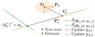
Figure 1: Graphical representation of two consecutive noise-free updates for a linear Kalman filter operating in 2D. The covariance matrix is represented by an ellipsoid where the true state lies with high probability, which becomes flat and aligned with the observed set after a perfect measurement is made.

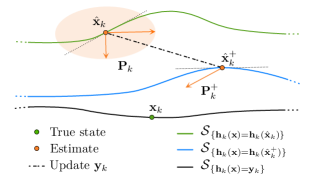
Figure 2: Graphical representation of EKF issues with Property 1. The level curves of $h$ are represented, and the observed set is the bottom one. 1) we see the EKF update $\hat{\mathbf{x}}_{k}^{+}$ fails to “land” on the observed set, so that (22) fails to hold. 2) in terms of updated uncertainty ellipsoid, it righteously becomes flat, owing to sure information. Besides, tangential directions to level curves at $\hat{\mathbf{x}}_{k}$ are $\ker\mathbf{H}_{k}$, with $\mathbf{H}_{k}=\mathbf{h}^{\prime}(\hat{\mathbf{x}}_{k})$. The tangent directions at updated state $\hat{\mathbf{x}}_{k}^{+}$, given by $\ker\mathbf{H}_{k}^{+}$, differ. As the EKF linearizes at point $\hat{\mathbf{x}}_{k}$ to perform its update, we have $\mathbf{H}_{k}\mathbf{P}_{k}^{+}\mathbf{H}_{k}^{T}=0$, but no information about $\hat{\mathbf{x}}_{k}^{+}$ is used, and $\mathbf{H}_{k}^{+}\mathbf{P}_{k}^{+}(\mathbf{H}_{k}^{+})^{T}\neq 0$. Thus, (23) also fails to hold.

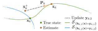
Figure 3: Graphical representation of EKF issues with Property 2. The EKF initial belief is assumed compatible with a prior noise-free measurement, i.e., $\mathbf{h}_{k,1}(\hat{\mathbf{x}}_{k})=\mathbf{y}_{1}$ and $\mathbf{H}_{1}\mathbf{P}_{k}\mathbf{H}_{1}^{T}=\mathbf{0}$ with $\mathbf{H}_{1}=\mathbf{h}_{k,1}^{\prime}(\hat{\mathbf{x}}_{k})$. Any immediately subsequent observation should maintain the estimate within the observed set $\mathbf{h}_{k,1}(\mathbf{x})=\mathbf{y}_{k,1}$, as the information is sure. Contrary to the linear KF, though, $\mathbf{P}_{k}$ only captures infinitesimal variability. Thus, when trying to incorporate a different measurement $\mathbf{y}_{k,2}$, although the EKF update points to a meaningful direction locally, the nonlinear nature of the observed set makes the updated estimate step out of it.

4 The iterated invariant extended Kalman filter (IIEKF)

The invariant extended Kalman filter (IEKF) of [13] exactly handles the nonlinear dynamics of group affine systems when process noise tends to zero, owing to the so-called log-linearity property. Regarding updates, there is no counterpart of such an exact property: the IEKF only provides approximations when it updates its belief with a left- or right-invariant measurement, and this even if measurement noise tends to zero. The present paper aims at improving the IEKF to obtain such properties.

4.1 The invariant EKF (IEKF)

Consider a state $\raisebox{1.0pt}{$\boldsymbol{\chi}$}_{k}$ evolving in a Lie group $G$. We assume $G$ is a matrix Lie group ($\raisebox{1.0pt}{$\boldsymbol{\chi}$}_{k}\in\mathbb{R}^{N\times N}$) with the matrix multiplication as composition law. As this operation is not commutative, the IEKF can be designed following the left- or right-invariant formalism, depending on whether one is dealing with left-invariant or right-invariant measurements. In this paper, we focus on the left-IEKF, the right-IEKF “mirroring” the latter, see [14]. The state is defined through the following nonlinear system

$$\raisebox{1.0pt}{$\boldsymbol{\chi}$}_{k+1} =\mathbf{f}(\raisebox{1.0pt}{$\boldsymbol{\chi}$}_{k},\mathbf{u}_{k})\exp_{G}(\mathbf{w}_{k}),$$ (24a)

$$\mathbf{y}_{k} =\raisebox{1.0pt}{$\boldsymbol{\chi}$}_{k}\mathbf{d}_{k}+\mathbf{n}_{k},$$ (24b)

where $\mathbf{u}_{k}\in\mathbb{R}^{m}$ is the system input, $\mathbf{d}_{k}\in\mathbb{R}^{N}$, $\mathbf{w}_{k}\sim\mathcal{N}(\mathbf{0},\mathbf{Q}_{k})$ is the process noise, and $\mathbf{n}_{k}\sim\mathcal{N}(\mathbf{0},\mathbf{N}_{k})$ is the measurement noise. The IEKF seeks to estimate $\raisebox{1.0pt}{$\boldsymbol{\chi}$}_{k}$.

Uncertainty representation

The left-IEKF defines the nonlinear error

$$\boldsymbol{\eta}_{k}=\hat{\raisebox{1.0pt}{$\boldsymbol{\chi}$}}_{k}^{-1}\raisebox{1.0pt}{$\boldsymbol{\chi}$}_{k}=\exp_{G}(\boldsymbol{\xi}_{k}),$$ (25)

where $\exp_{G}$ is the exponential map of Lie group $G$, and where $\boldsymbol{\xi}_{k}\in\mathbb{R}^{n}$ is called the linearized error. The linearized error is assumed to follow a Gaussian distribution, so that the state follows a concentrated Gaussian distribution on $G$, centered on the current estimate $\hat{\raisebox{1.0pt}{$\boldsymbol{\chi}$}}_{k}$ [31, 32, 33, 34], that is,

$$\raisebox{1.0pt}{$\boldsymbol{\chi}$}_{k}=\hat{\raisebox{1.0pt}{$\boldsymbol{\chi}$}}_{k}\exp_{G}(\boldsymbol{\xi}_{k}),\quad\text{with $\boldsymbol{\xi}_{k}\sim\mathcal{N}(\mathbf{0},\mathbf{P}_{k})$}.$$ (26)

In this formula, which is a Lie group analog to (18), $\hat{\raisebox{1.0pt}{$\boldsymbol{\chi}$}}_{k}$ represents the noise-free “mean” of the Gaussian, and the dispersion arises by multiplying it with the random matrix $\exp_{G}(\boldsymbol{\xi}_{k})$, see e.g., [14].

Propagation

The belief is propagated through dynamics (24a) with no process noise. The linearized error thus evolves as $\boldsymbol{\xi}_{k+1}=\mathbf{F}_{k}\boldsymbol{\xi}_{k}+\mathbf{G}_{k}\mathbf{w}_{k},$ so that

$$\hat{\raisebox{1.0pt}{$\boldsymbol{\chi}$}}_{k+1} =\mathbf{f}(\hat{\raisebox{1.0pt}{$\boldsymbol{\chi}$}}_{k},\mathbf{u}_{k}),$$ (27a)

$$\mathbf{P}_{k+1} =\mathbf{F}_{k}\mathbf{P}_{k}\mathbf{F}_{k}^{T}+\mathbf{G}_{k}\mathbf{Q}_{k}\mathbf{G}_{k}^{T},$$ (27b)

with $\mathbf{F}_{k}$, $\mathbf{G}_{k}$ the Jacobians w.r.t. the chosen linearized error and the process noise, see [14], evaluated at $(\hat{\raisebox{1.0pt}{$\boldsymbol{\chi}$}}_{k},\mathbf{u}_{k},\mathbf{0})$. Note that the method developed in this paper does not require the function $\mathbf{f}$ to be group affine, i.e., it does not need to satisfy (11) in [14].

Update

Measurement (24b) brings partial information about the current error $\boldsymbol{\xi}_{k}$. In the (left) invariant filtering framework, the innovation (prediction error) is defined as

$$\mathbf{z}_{k} =\hat{\raisebox{1.0pt}{$\boldsymbol{\chi}$}}_{k}^{-1}\mathbf{y}_{k}-\mathbf{d}_{k},$$ (28a)

$$=\exp_{G}(\boldsymbol{\xi}_{k})\mathbf{d}_{k}-\mathbf{d}_{k}+\hat{\raisebox{1.0pt}{$\boldsymbol{\chi}$}}_{k}^{-1}\mathbf{n}_{k},$$ (28b)

$$=\mathbf{H}_{k}\boldsymbol{\xi}_{k}+\raisebox{1.0pt}{$\boldsymbol{\chi}$}_{k}^{-1}\mathbf{n}_{k}+\mathcal{O}(\|\boldsymbol{\xi}_{k}\|^{2}),$$ (28c)

where $\mathbf{H}_{k}$ is the invariant filtering output Jacobian

$$\exp_{G}(\boldsymbol{\xi})\mathbf{d}_{k}=\mathbf{d}_{k}+\mathbf{H}_{k}\boldsymbol{\xi}+\mathcal{O}(\|\boldsymbol{\xi}\|^{2}).$$ (29)

associated to map $\mathbf{h}_{k}(\raisebox{1.0pt}{$\boldsymbol{\chi}$})=\raisebox{1.0pt}{$\boldsymbol{\chi}$}\mathbf{d}_{k}$, whose mathematical expression will be recalled at (46). A flagship property of invariant filtering is that, owing to the form of the output, the Jacobian $\mathbf{H}_{k}$ does not depend on the current estimate $\hat{\raisebox{1.0pt}{$\boldsymbol{\chi}$}}_{k}$ (only on $\mathbf{d}_{k}$), see (28b). In the light of measurement $\mathbf{y}_{k}$, the (left) IEKF [13] updates its belief according to

$$\mathbf{K}_{k} =\mathbf{P}_{k}\mathbf{H}_{k}^{T}(\mathbf{H}_{k}\mathbf{P}_{k}\mathbf{H}_{k}^{T}+\hat{\mathbf{N}}_{k})^{-1},$$ (30a)

$$\boldsymbol{\xi}_{k}^{+} =\mathbf{K}_{k}\mathbf{z}_{k},$$ (30b)

$$\hat{\raisebox{1.0pt}{$\boldsymbol{\chi}$}}_{k}^{+} =\hat{\raisebox{1.0pt}{$\boldsymbol{\chi}$}}_{k}\exp_{G}(\boldsymbol{\xi}_{k}^{+}),$$ (30c)

$$\mathbf{P}_{k}^{+} =(\mathbf{I}-\mathbf{K}_{k}\mathbf{H}_{k})\mathbf{P}_{k},$$ (30d)

where $\hat{\mathbf{N}}_{k}=\hat{\raisebox{1.0pt}{$\boldsymbol{\chi}$}}_{k}^{-1}\mathbf{N}_{k}(\hat{\raisebox{1.0pt}{$\boldsymbol{\chi}$}}_{k}^{-1})^{T}$.

4.2 Derivation of the iterated invariant EKF (IIEKF)

In this paper, we introduce the iterated IEKF, that attempts to solve the MAP problem by using the GN method.

Proposition 1.

Starting from the prior (26), supposed to encode the state distribution conditional on past information $\mathbf{y}_{0},\ldots,\mathbf{y}_{k-1}$, the MAP estimate in the light of latest measurement $\mathbf{y}_{k}$ is given by $\hat{\raisebox{1.0pt}{$\boldsymbol{\chi}$}}_{k}^{\star}=\hat{\raisebox{1.0pt}{$\boldsymbol{\chi}$}}_{k}\exp_{G}(\boldsymbol{\xi}_{k}^{\star})$, where $\boldsymbol{\xi}_{k}^{\star}$ is the solution to the optimization problem

$$\boldsymbol{\xi}_{k}^{\star}=\operatorname*{argmin}\limits_{\boldsymbol{\xi}}\frac{1}{2}\|\boldsymbol{\xi}\|^{2}_{\mathbf{P}_{k}}+\frac{1}{2}\|\mathbf{z}_{k}-\exp_{G}(\boldsymbol{\xi})\mathbf{d}_{k}+\mathbf{d}_{k}\|^{2}_{\hat{\mathbf{N}}_{k}}.$$ (31)

Proof.

We have

$$p(\boldsymbol{\xi}_{k}\mid\mathbf{y}_{k}) =p(\boldsymbol{\xi}_{k}\mid\mathbf{z}_{k})\propto p(\mathbf{z}_{k}\mid\boldsymbol{\xi}_{k})p(\boldsymbol{\xi}_{k}),$$ (32)

with all densities $p$ implicitly conditional on past information $\mathbf{y}_{0},\ldots,\mathbf{y}_{k-1}$. Then, the density $p(\boldsymbol{\xi}_{k}\mid\mathbf{y}_{k})$ is proportional to $\exp(-\frac{1}{2}\|\boldsymbol{\xi}_{k}\|^{2}_{\mathbf{P}_{k}})\exp(-\frac{1}{2}\|\mathbf{z}_{k}-\exp_{G}(\boldsymbol{\xi}_{k})\mathbf{d}_{k}+\mathbf{d}_{k}\|^{2}_{\hat{\mathbf{N}}_{k}})$. ∎

Akin to the conventional iterated EKF [3], we intend to solve (31) iteratively using the GN method. All we need to do is linearize the Lie exponential.

Lemma 2.

We have the following first-order expansion

$$\exp_{G}(\bar{\boldsymbol{\xi}}+\boldsymbol{\delta})\mathbf{d}=\exp_{G}(\bar{\boldsymbol{\xi}})\mathbf{d}+\exp_{G}(\bar{\boldsymbol{\xi}})\mathbf{H}_{k}\mathbf{\mathcal{J}}_{r}(\bar{\boldsymbol{\xi}})\boldsymbol{\delta}+\|\boldsymbol{\delta}\|^{2},$$ (33)

with $\mathbf{H}_{k}$ as in (29), and where the right Lie Jacobian  [31] is defined by $\exp_{G}(\boldsymbol{\xi}+\boldsymbol{\delta})\approx\exp_{G}(\boldsymbol{\xi})\exp_{G}(\mathbf{\mathcal{J}}_{r}(\boldsymbol{\xi})\boldsymbol{\delta})$ neglecting terms of order $\|\boldsymbol{\delta}\|^{2}$. Its expression is given in Appendix B.

Proof.

We have the first-order expansion in $\boldsymbol{\delta}$

$$\exp_{G}(\bar{\boldsymbol{\xi}}+\boldsymbol{\delta})\mathbf{d} \approx\exp_{G}(\bar{\boldsymbol{\xi}})\exp_{G}(\mathbf{\mathcal{J}}_{r}(\bar{\boldsymbol{\xi}})\boldsymbol{\delta})\mathbf{d},$$ (34a)

$$\approx\exp_{G}(\bar{\boldsymbol{\xi}})\big{(}\mathbf{d}+\mathbf{H}_{k}\mathbf{\mathcal{J}}_{r}(\bar{\boldsymbol{\xi}})\boldsymbol{\delta}\big{)}.$$ (34b)

where we applied (29) with $\boldsymbol{\xi}=\mathbf{\mathcal{J}}_{r}(\bar{\boldsymbol{\xi}})\boldsymbol{\delta}.$ ∎

Now, letting $\mathbf{b}:=\mathbf{z}_{k}+\mathbf{d}_{k}$, $\bar{\mathbf{h}}(\boldsymbol{\xi}):=\exp_{G}(\boldsymbol{\xi})\mathbf{d}_{k}$, and $\bar{\mathbf{x}}=\mathbf{0}$, we see objectives (31) and (8) coincide, so that a direct application of Lemma 1 of Section 2.4 and Lemma 2 yields the following proposition.

Proposition 2.

The sequence of GN updates for the optimization problem (31) writes

$$\boldsymbol{\xi}_{k}^{i+1}=\mathbf{K}_{k}^{i}\big{(}\mathbf{z}_{k}-\exp_{G}(\boldsymbol{\xi}_{k}^{i})\mathbf{d}_{k}+\mathbf{d}_{k}+\mathbf{H}_{k}^{i}\boldsymbol{\xi}_{k}^{i}\big{)},$$ (35)

letting $\mathbf{H}_{k}$ be the IEKF’s standard Jacobian and

$$\mathbf{H}_{k}^{i} =\exp_{G}(\boldsymbol{\xi}_{k}^{i})\mathbf{H}_{k}\mathbf{\mathcal{J}}_{r}(\boldsymbol{\xi}_{k}^{i}),$$ (36)

$$\mathbf{K}_{k}^{i} =\mathbf{P}_{k}(\mathbf{H}_{k}^{i})^{T}\left(\mathbf{H}_{k}^{i}\mathbf{P}_{k}(\mathbf{H}_{k}^{i})^{T}+\hat{\mathbf{N}}_{k}\right)^{-1}.$$ (37)

Assuming the GN method converges after $i^{\star}$ iterations, the IIEKF eventually updates its estimate following the IEKF methodology (30c), i.e.,

$$\hat{\raisebox{1.0pt}{$\boldsymbol{\chi}$}}_{k}^{+}=\hat{\raisebox{1.0pt}{$\boldsymbol{\chi}$}}_{k}\exp_{G}\left(\boldsymbol{\xi}_{k}^{i^{\star}}\right).$$ (38)

Since Jacobian $\mathbf{H}_{k}$ is independent from the current estimate, the Riccati update does not require any iteration, and the IIEKF updates its error covariance once and for all as follows

$$\mathbf{P}_{k}^{+}=(\mathbf{I}-\mathbf{K}_{k}\mathbf{H}_{k})\mathbf{P}_{k},$$ (39)

with $\mathbf{H}_{k}=\mathbf{H}_{k}^{0}$ and $\mathbf{K}_{k}=\mathbf{K}_{k}^{0}$. The full algorithm is summarized in Algorithm 1, and we see we exactly recover the IEKF of [13] if we perform one iteration only.

Algorithm 1 The iterated invariant extended Kalman filter (IIEKF)

1:  Choose the initial state $\hat{\raisebox{1.0pt}{$\boldsymbol{\chi}$}}_{0}\in G$ and initial covariance $\mathbf{P}_{0}=\mathrm{Cov}(\boldsymbol{\xi}_{0})\in\mathbb{R}^{n\times n}$.

2:  loop

3:     Define dynamics Jacobian $\mathbf{F}_{k}$ of IEKF framework.

4:     Define dynamics Jacobian $\mathbf{G}_{k}$ w.r.t. process noise.

5:     Define output Jacobian $\mathbf{H}_{k}$ of IEKF framework [13].

6:     Define process noise covariance $\mathbf{Q}_{k}$.

7:     Define measurement noise covariance $\mathbf{N}_{k}$.

8:     

9:     {Measurement update}

10:     $\mathrlap{i}\hphantom{\Delta\boldsymbol{\xi}_{k}^{i}}\leftarrow 0$

11:     $\mathrlap{\boldsymbol{\xi}_{k}^{i}}\hphantom{\Delta\boldsymbol{\xi}_{k}^{i}}\leftarrow\mathbf{0}$

12:     $\mathrlap{\Delta\boldsymbol{\xi}_{k}^{i}}\hphantom{\Delta\boldsymbol{\xi}_{k}^{i}}\leftarrow+\infty$

13:     $\mathrlap{\mathbf{z}_{k}}\hphantom{\Delta\boldsymbol{\xi}_{k}^{i}}\leftarrow\hat{\raisebox{1.0pt}{$\boldsymbol{\chi}$}}_{k}^{-1}\mathbf{y}_{k}-\mathbf{d}_{k}$

14:     $\mathrlap{\mathbf{z}_{k}^{i}}\hphantom{\Delta\boldsymbol{\xi}_{k}^{i}}\leftarrow\mathbf{z}_{k}$

15:     $\mathrlap{\hat{\mathbf{N}}_{k}}\hphantom{\Delta\boldsymbol{\xi}_{k}^{i}}\leftarrow\hat{\raisebox{1.0pt}{$\boldsymbol{\chi}$}}_{k}^{-1}\mathbf{N}_{k}(\hat{\raisebox{1.0pt}{$\boldsymbol{\chi}$}}_{k}^{-1})^{T}$

16:     while $\Delta\boldsymbol{\xi}_{k}^{i}>\mathrm{tol}$ and $i<N_{\mathrm{max}}$ do

17:        $\mathrlap{\mathbf{H}_{k}^{i}}\hphantom{\Delta\boldsymbol{\xi}_{k}^{i}}\leftarrow\exp_{G}\left(\boldsymbol{\xi}_{k}^{i}\right)\mathbf{H}_{k}\mathbf{\mathcal{J}}_{r}(\boldsymbol{\xi}_{k}^{i})$

18:        $\mathrlap{\mathbf{K}_{k}^{i}}\hphantom{\Delta\boldsymbol{\xi}_{k}^{i}}\leftarrow\mathbf{P}_{k}(\mathbf{H}_{k}^{i})^{T}(\mathbf{H}_{k}^{i}\mathbf{P}_{k}(\mathbf{H}_{k}^{i})^{T}+\hat{\mathbf{N}}_{k})^{-1}$

19:        $\mathrlap{\mathbf{z}_{k}^{i}}\hphantom{\Delta\boldsymbol{\xi}_{k}^{i}}\leftarrow\mathbf{z}_{k}-\exp_{G}(\boldsymbol{\xi}^{i})\mathbf{d}_{k}+\mathbf{d}_{k}+\mathbf{H}_{k}^{i}\boldsymbol{\xi}_{k}^{i}$

20:        $\mathrlap{\Delta\boldsymbol{\xi}_{k}^{i}}\hphantom{\Delta\boldsymbol{\xi}_{k}^{i}}\leftarrow\|\mathbf{K}_{k}^{i}\mathbf{z}_{k}^{i}-\boldsymbol{\xi}_{k}^{i}\|$

21:        $\mathrlap{\boldsymbol{\xi}_{k}^{i}}\hphantom{\Delta\boldsymbol{\xi}_{k}^{i}}\leftarrow\mathbf{K}_{k}^{i}\mathbf{z}_{k}^{i}$

22:        $\mathrlap{i}\hphantom{\Delta\boldsymbol{\xi}_{k}^{i}}\leftarrow i+1$

23:     end while

24:     $\mathrlap{\hat{\raisebox{1.0pt}{$\boldsymbol{\chi}$}}_{k}^{+}}\hphantom{\Delta\boldsymbol{\xi}_{k}^{i}}\leftarrow\hat{\raisebox{1.0pt}{$\boldsymbol{\chi}$}}_{k}\exp_{G}\left(\boldsymbol{\xi}_{k}^{i}\right)$

25:     $\mathrlap{\mathbf{K}_{k}}\hphantom{\Delta\boldsymbol{\xi}_{k}^{i}}\leftarrow\mathbf{P}_{k}\mathbf{H}_{k}^{T}(\mathbf{H}_{k}\mathbf{P}_{k}\mathbf{H}_{k}^{T}+\hat{\mathbf{N}}_{k})^{-1}$

26:     $\mathrlap{\mathbf{P}_{k}^{+}}\hphantom{\Delta\boldsymbol{\xi}_{k}^{i}}\leftarrow(\mathbf{I}-\mathbf{K}_{k}\mathbf{H}_{k})\mathbf{P}_{k}$

27:     

28:     {Propagation}

29:     $\mathrlap{\hat{\raisebox{1.0pt}{$\boldsymbol{\chi}$}}_{k+1}}\hphantom{\hat{\raisebox{1.0pt}{$\boldsymbol{\chi}$}}_{k+1}}\leftarrow\mathbf{f}(\hat{\raisebox{1.0pt}{$\boldsymbol{\chi}$}}_{k}^{+},\mathbf{u}_{k})$

30:     $\mathrlap{\mathbf{P}_{k+1}}\hphantom{\hat{\raisebox{1.0pt}{$\boldsymbol{\chi}$}}_{k+1}}\leftarrow\mathbf{F}_{k}\mathbf{P}_{k}^{+}\mathbf{F}_{k}^{T}+\mathbf{G}_{k}\mathbf{Q}_{k}\mathbf{G}_{k}^{T}$

31:  end loop

5 Theoretical properties of the IIEKF

Consider the left-invariant measurement (24b). Deriving properties in the presence of measurement noise seems out of reach, as is often the case in nonlinear filtering (e.g., the log-linear error property of [13] holds in the absence of process noise). However, in the degenerate case where the magnitude of the measurement noise tends to zero (whereas the state estimate and the propagation may be noisy), we will show the desirable properties of the linear case, outlined in Subsection 3.2, hold. This provides strong guarantees when using an IIEKF with noise-free or pseudo measurements, as in the application below. Besides, as there is a continuum between the noise-free and the noisy cases, the properties approximately hold in the case of small measurement noise.

5.1 The IIEKF in the face of noise-free measurements

To derive mathematical properties, we need to understand how the proposed IIEKF behaves when measurement noise vanishes. Let $\hat{\mathbf{N}}_{k}=\delta\mathbf{I}$, with $\delta\ll 1$. In this context, Problem (31) becomes that of minimizing $f_{\delta}(\boldsymbol{\xi})=\frac{1}{2}\|\boldsymbol{\xi}\|^{2}_{\mathbf{P}_{k}}+\frac{1}{2}\|\mathbf{z}_{k}-\exp_{G}(\boldsymbol{\xi})\mathbf{d}_{k}+\mathbf{d}_{k}\|^{2}_{\delta\mathbf{I}}$. The minimizer of $f_{\delta}$ may be sought using the GN sequence of estimates of Proposition 2

$$\boldsymbol{\xi}_{k,\delta}^{i+1} =\mathbf{K}_{k,\delta}^{i}\cdot\underbrace{\left(\mathbf{z}_{k}-\exp_{G}(\boldsymbol{\xi}_{k,\delta}^{i})\mathbf{d}_{k}+\mathbf{d}_{k}+\mathbf{H}_{k,\delta}^{i}\boldsymbol{\xi}_{k,\delta}^{i}\right)}_{\mathbf{z}_{k,\delta}^{i}},$$ (40)

where $\mathbf{H}_{k,\delta}^{i}=\exp_{G}(\boldsymbol{\xi}_{k,\delta}^{i})\mathbf{H}_{k}\mathbf{\mathcal{J}}_{r}(\boldsymbol{\xi}_{k,\delta}^{i})$ and where we let $\mathbf{K}_{k,\delta}^{i}=\mathbf{P}_{k}(\mathbf{H}_{k,\delta}^{i})^{T}\left(\mathbf{H}_{k,\delta}^{i}\mathbf{P}_{k}(\mathbf{H}_{k,\delta}^{i})^{T}+\delta\mathbf{I}\right)^{-1}$. Starting from $\boldsymbol{\xi}_{k,\delta}^{0}=\mathbf{0}$ and taking the limit for $\delta\rightarrow 0$, we get

$$\lim\limits_{\delta\rightarrow 0}\boldsymbol{\xi}_{k,\delta}^{i+1} =\lim\limits_{\delta\rightarrow 0}\mathbf{K}_{k,\delta}^{i}\cdot\lim\limits_{\delta\rightarrow 0}\mathbf{z}_{k,\delta}^{i},$$ (41)

so that the GN sequence approximating the solution to the noise-free optimization problem becomes

$$\boldsymbol{\xi}_{k}^{i+1}=\mathbf{L}_{k}(\mathbf{H}_{k}^{i}\mathbf{L}_{k})^{\dagger}\mathbf{z}_{k}^{i},$$ (42)

recalling (14). This provides the following limit IIEKF for noise-free measurements, described in Algorithm 2.

Algorithm 2 The iterated invariant extended Kalman filter (IIEKF) with noise-free measurements

  Same as Algorithm 1 with the following exceptions.

  Line 18: $\mathrlap{\mathbf{K}_{k}^{i}}\hphantom{\Delta\boldsymbol{\xi}_{k}^{i}}\leftarrow\mathbf{L}_{k}(\mathbf{H}_{k}^{i}\mathbf{L}_{k})^{\dagger}$

  Line 25: $\mathrlap{\mathbf{K}_{k}}\hphantom{\Delta\boldsymbol{\xi}_{k}^{i}}\leftarrow\mathbf{L}_{k}(\mathbf{H}_{k}\mathbf{L}_{k})^{\dagger}$

  Line 26: $\mathrlap{\mathbf{P}_{k}^{+}}\hphantom{\Delta\boldsymbol{\xi}_{k}^{i}}\leftarrow(\mathbf{I}-\mathbf{K}_{k}\mathbf{H}_{k})\mathbf{P}_{k}$

This algorithm is not in our preliminary conference paper [30], where we derived an heuristic noise-free IEKF instead.

5.2 The IIEKF satisfies the compatibility property

Having derived the limit-case IIEKF, we may prove it satisfies the desirable Property 1 enunciated above.

5.2.1 First part (the estimate lands on the right subspace)

We start by discussing the first part of the property, namely desirable Equation (22). As measurement noise tends to $\mathbf{0}$, Problem (31) becomes that of finding the smallest $\boldsymbol{\xi}$ in the sense of the metric induced by $\mathbf{P}_{k}$ that satisfies the hard constraint $\|\mathbf{z}_{k}-\exp_{G}(\boldsymbol{\xi})\mathbf{d}_{k}+\mathbf{d}_{k}\|^{2}=0$, which boils down to $\hat{\raisebox{1.0pt}{$\boldsymbol{\chi}$}}_{k}^{-1}\mathbf{y}_{k}=\exp_{G}\left(\boldsymbol{\xi}\right)\mathbf{d}_{k}$, see (28b). We thus have $\hat{\raisebox{1.0pt}{$\boldsymbol{\chi}$}}_{k}\exp_{G}\left(\boldsymbol{\xi}_{k}^{\star}\right)\mathbf{d}_{k}=\mathbf{y}_{k}$, where $\boldsymbol{\xi}_{k}^{\star}$ is the $\operatorname*{argmin}$ we search for. As long as IIEKF’s iterate $\boldsymbol{\xi}_{k}^{i}$ converges to it, the updated state $\hat{\raisebox{1.0pt}{$\boldsymbol{\chi}$}}_{k}^{+}=\hat{\raisebox{1.0pt}{$\boldsymbol{\chi}$}}_{k}\exp_{G}(\boldsymbol{\xi}_{k}^{\star})$ belongs to the observed set indeed, that is, $\hat{\raisebox{1.0pt}{$\boldsymbol{\chi}$}}_{k}^{+}\in\mathcal{S}_{\{\raisebox{1.0pt}{$\boldsymbol{\chi}$}\mathbf{d}_{k}=\mathbf{y}_{k}\}}$.

Of course, this assumes the GN descent converges to a global minimizer. As the optimization problem is not convex, the GN sequence (42) converges towards the global minimizer provided that the true error $\boldsymbol{\xi}_{k}$ is close enough to $\mathbf{0}$. It is important to note that a non-iterative update scheme, like the IEKF update, has no chance to satisfy $\hat{\raisebox{1.0pt}{$\boldsymbol{\chi}$}}_{k}^{+}\in\mathcal{S}_{\{\raisebox{1.0pt}{$\boldsymbol{\chi}$}\mathbf{d}_{k}=\mathbf{y}_{k}\}}$.

5.2.2 Second part (the covariance correctly encodes the uncertainty drop)

The second part of Property 1, namely desirable Equation (23), is proved by the following result.

Theorem 1.

For noise-free measurements expressed in the left-invariant (or right-invariant) form, that is, $\mathbf{y}_{k}=\raisebox{1.0pt}{$\boldsymbol{\chi}$}_{k}\mathbf{d}_{k}$ (or $\mathbf{y}_{k}=\raisebox{1.0pt}{$\boldsymbol{\chi}$}_{k}^{-1}\mathbf{d}_{k}$), the invariant framework naturally ensures $\mathbf{H}_{k}^{+}\mathbf{P}_{k}^{+}(\mathbf{H}_{k}^{+})^{T}=\mathbf{0}$, and also $\mathbf{H}_{k}\mathbf{P}_{k}^{+}(\mathbf{H}_{k})^{T}=\mathbf{0}$.

Proof.

From the theory of invariant filtering, left- or right-invariant measurements yield a Jacobian $\mathbf{H}_{k}$ that is independent from the current estimate, see [14], meaning that $\mathbf{H}_{k}=\mathbf{H}_{k}^{+}$, which is the key property. This property is reminiscent of the linear Kalman filter, so that the same results hold. Either 1) $\mathbf{H}_{k}\mathbf{P}_{k}\mathbf{H}_{k}^{T}$ is invertible, and thus $\mathbf{H}_{k}\mathbf{P}_{k}^{+}\mathbf{H}_{k}^{T}=\mathbf{H}_{k}\big{(}(\mathbf{I}-\mathbf{P}_{k}\mathbf{H}_{k}^{T}(\mathbf{H}_{k}\mathbf{P}_{k}\mathbf{H}_{k}^{T})^{-1}\mathbf{H}_{k})\mathbf{P}_{k})\big{)}\mathbf{H}_{k}^{T}=\mathbf{0}$ or 2) the same calculation (67) as in the linear case then holds. ∎

5.3 The IIEKF’s belief is strongly compatible

Before we turn to desirable Property 2, we would like to underline that compatibility of the belief and the observed set is in fact very strong, as illustrated by the following result.

Proposition 3.

Under the compatibility assumptions of Definition 2, the entire probability distribution encoded by model (26) is in fact contained within the observed set. Mathematically, supposing the belief is compatible with noise-free measurement $\mathbf{y}_{k}=\raisebox{1.0pt}{$\boldsymbol{\chi}$}\mathbf{d}_{k}$, in the sense that

$$\hat{\raisebox{1.0pt}{$\boldsymbol{\chi}$}}_{k}\in\mathcal{S}_{\{\raisebox{1.0pt}{$\boldsymbol{\chi}$}\mathbf{d}_{k}=\mathbf{y}_{k}\}}\quad\text{and}\quad\mathbf{H}_{k}\mathbf{P}_{k}\mathbf{H}_{k}^{T}=\mathbf{0},$$ (43)

with $\mathbf{H}_{k}$ the Jacobian associated to $\mathbf{d}_{k}$, implies that for any $\boldsymbol{\xi}$ drawn from $\mathcal{N}(\mathbf{0},\mathbf{P}_{k})$, we have $\hat{\raisebox{1.0pt}{$\boldsymbol{\chi}$}}_{k}\exp_{G}(\boldsymbol{\xi})\in\mathcal{S}_{\{\raisebox{1.0pt}{$\boldsymbol{\chi}$}\mathbf{d}_{k}=\mathbf{y}_{k}\}}$.

The proof consists in noting that then $\boldsymbol{\xi}$ is (almost surely) in the column space of $\mathbf{P}_{k}$, hence $\mathbf{H}_{k}\boldsymbol{\xi}=\mathbf{0}$, and in using a key result from the invariant filtering theory [35, 36].

Lemma 3.

Let $\mathbf{H}_{k}$ denote the Jacobian from invariant filtering associated to map $\mathbf{h}_{k}(\raisebox{1.0pt}{$\boldsymbol{\chi}$})=\raisebox{1.0pt}{$\boldsymbol{\chi}$}\mathbf{d}_{k}$. We have

$$\begin{array}[]{c}\hat{\raisebox{1.0pt}{$\boldsymbol{\chi}$}}_{k}\in\mathcal{S}_{\{\raisebox{1.0pt}{$\boldsymbol{\chi}$}\mathbf{d}_{k}=\mathbf{y}_{k}\}}\quad\text{and}\quad\mathbf{H}_{k}\boldsymbol{\xi}=\mathbf{0},~{}\boldsymbol{\xi}\in\mathbb{R}^{n}\\ \Downarrow\\ \hat{\raisebox{1.0pt}{$\boldsymbol{\chi}$}}_{k}\exp_{G}\left(\boldsymbol{\xi}\right)\in\mathcal{S}_{\{\raisebox{1.0pt}{$\boldsymbol{\chi}$}\mathbf{d}_{k}=\mathbf{y}_{k}\}}.\end{array}$$ (44)

Proof.

Let $\mathcal{L}_{\mathfrak{g}}(\cdot):\mathbb{R}^{n}\rightarrow\mathfrak{g}$ be the bijective map between the vector space $\mathbb{R}^{n}$ and the Lie algebra $\mathfrak{g}$ of group $G$, see [13]. As we are dealing with matrix Lie groups, the exponential coincides with the matrix exponential in the following sense

$$\exp_{G}(\boldsymbol{\xi})=\mathbf{I}+\sum\limits_{l=1}^{+\infty}\frac{1}{l!}\mathcal{L}_{\mathfrak{g}}(\boldsymbol{\xi})^{l}.$$ (45)

Keeping only first-order terms proves, in passing, that Jacobian $\mathbf{H}_{k}$ from (28b) writes

$$\mathbf{H}_{k}\boldsymbol{\xi}=\mathcal{L}_{\mathfrak{g}}(\boldsymbol{\xi})\mathbf{d}_{k}.$$ (46)

To prove the result we seek, it then suffices to write

$$\hat{\raisebox{1.0pt}{$\boldsymbol{\chi}$}}_{k}\exp_{G}(\boldsymbol{\xi})\mathbf{d}_{k} =\hat{\raisebox{1.0pt}{$\boldsymbol{\chi}$}}_{k}\left(\mathbf{I}+\sum\limits_{l=1}^{+\infty}\frac{1}{l!}\mathcal{L}_{\mathfrak{g}}(\boldsymbol{\xi})^{l}\right)\mathbf{d}_{k},$$ (47a)

$$=\hat{\raisebox{1.0pt}{$\boldsymbol{\chi}$}}_{k}\mathbf{d}_{k}+\hat{\raisebox{1.0pt}{$\boldsymbol{\chi}$}}_{k}\sum\limits_{l=1}^{+\infty}\frac{1}{l!}\mathcal{L}_{\mathfrak{g}}(\boldsymbol{\xi})^{l}\mathbf{d}_{k},$$ (47b)

$$=\hat{\raisebox{1.0pt}{$\boldsymbol{\chi}$}}_{k}\mathbf{d}_{k}+\hat{\raisebox{1.0pt}{$\boldsymbol{\chi}$}}_{k}\sum\limits_{l=1}^{+\infty}\frac{1}{l!}\mathcal{L}_{\mathfrak{g}}(\boldsymbol{\xi})^{l-1}\left(\mathcal{L}_{\mathfrak{g}}(\boldsymbol{\xi})\mathbf{d}_{k}\right).$$ (47c)

Since $\mathbf{H}_{k}\boldsymbol{\xi}=\mathcal{L}_{\mathfrak{g}}(\boldsymbol{\xi})\mathbf{d}_{k}=\mathbf{0}$ and $\hat{\raisebox{1.0pt}{$\boldsymbol{\chi}$}}_{k}\in\mathcal{S}_{\{\raisebox{1.0pt}{$\boldsymbol{\chi}$}\mathbf{d}_{k}=\mathbf{y}_{k}\}}$, the last line gives

$$\hat{\raisebox{1.0pt}{$\boldsymbol{\chi}$}}_{k}\exp_{G}(\boldsymbol{\xi})\mathbf{d}_{k}=\hat{\raisebox{1.0pt}{$\boldsymbol{\chi}$}}_{k}\mathbf{d}_{k}=\mathbf{y}_{k},$$ (48)

which proves $\hat{\raisebox{1.0pt}{$\boldsymbol{\chi}$}}_{k}\exp_{G}(\boldsymbol{\xi})\in\mathcal{S}_{\{\raisebox{1.0pt}{$\boldsymbol{\chi}$}\mathbf{d}_{k}=\mathbf{y}_{k}\}}$. ∎

The result of Proposition 3 shows that the local information encoded by the IEKF is in fact global, exactly as in the linear case, where a Gaussian vector with rank-deficient covariance matrix has a distribution that is entirely contained within a linear subspace.

5.4 The IIEKF satisfies the “hard encoding” property

We now have what we need to actually show that the IIEKF possesses desirable Property 2: the filter inherently “hard codes” deterministic information.

Theorem 2.

Consider a (left) IIEKF whose belief $(\hat{\raisebox{1.0pt}{$\boldsymbol{\chi}$}}_{k},\mathbf{P}_{k})$ is compatible in the sense of Definition 2 with measurement (24b) with noise turned off, i.e., $\mathbf{y}_{k}=\raisebox{1.0pt}{$\boldsymbol{\chi}$}_{k}\mathbf{d}_{k}$. This means $\hat{\raisebox{1.0pt}{$\boldsymbol{\chi}$}}_{k}\in\mathcal{S}_{\{\raisebox{1.0pt}{$\boldsymbol{\chi}$}\mathbf{d}_{k}=\mathbf{y}_{k}\}}$ and $\mathbf{H}_{k}\mathbf{P}_{k}\mathbf{H}_{k}^{T}=\mathbf{0}$ with $\mathbf{H}_{k}$ the Jacobian associated with $\mathbf{d}_{k}$. Then, if we immediately make another measurement $\tilde{\mathbf{y}}_{k}$, no matter its expression, the updated belief $(\hat{\raisebox{1.0pt}{$\boldsymbol{\chi}$}}_{k}^{+},\mathbf{P}_{k}^{+})$ corresponding to measurement $\tilde{\mathbf{y}}_{k}$ remains compatible with the (first) noise-free measurement. Mathematically,

$$\begin{array}[]{c}\hat{\raisebox{1.0pt}{$\boldsymbol{\chi}$}}_{k}\in\mathcal{S}_{\{\raisebox{1.0pt}{$\boldsymbol{\chi}$}\mathbf{d}_{k}=\mathbf{y}_{k}\}}\quad\text{and}\quad\mathbf{H}_{k}\mathbf{P}_{k}\mathbf{H}_{k}^{T}=\mathbf{0},\\ \Downarrow\\ \hat{\raisebox{1.0pt}{$\boldsymbol{\chi}$}}_{k}^{+}\in\mathcal{S}_{\{\raisebox{1.0pt}{$\boldsymbol{\chi}$}\mathbf{d}_{k}=\mathbf{y}_{k}\}}\quad\text{and}\quad\mathbf{H}_{k}\mathbf{P}_{k}^{+}\mathbf{H}_{k}^{T}=\mathbf{0}.\end{array}$$ (49)

Proof.

Point 2) of Definition 2 is the easiest to prove. If we have $\mathbf{H}_{k}\mathbf{P}_{k}\mathbf{H}_{k}^{T}=\mathbf{0}$, by symmetry it means $\mathbf{P}_{k}\mathbf{H}_{k}^{T}=\mathbf{0}$. Any immediately subsequent update of the IIEKF, see line 26 of Algorithm 1, writes $\mathrlap{\mathbf{P}_{k}^{+}}\hphantom{\Delta\boldsymbol{\xi}_{k}^{i}}=(\mathbf{I}-\mathbf{K}_{k}\tilde{\mathbf{H}}_{k})\mathbf{P}_{k}$, hence ${\mathbf{P}_{k}^{+}}$ verifies the same property whatever $\tilde{\mathbf{H}}_{k}$. And we have also ${\mathbf{H}_{k}^{+}}\mathbf{P}_{k}^{+}{\mathbf{H}_{k}^{+}}^{T}=\mathbf{0}$ owing to $\mathbf{H}_{k}={\mathbf{H}_{k}^{+}}.$

Regarding part 1), we see at line 24 of Algorithm 1 that the update writes $\mathrlap{\hat{\raisebox{1.0pt}{$\boldsymbol{\chi}$}}_{k}^{+}}\hphantom{\Delta\boldsymbol{\xi}_{k}^{i}}=\hat{\raisebox{1.0pt}{$\boldsymbol{\chi}$}}_{k}\exp_{G}\left(\boldsymbol{\xi}_{k}^{i}\right)$. Using Lemma 3, we see that provided $\boldsymbol{\xi}_{k}^{i}$ satisfies $\mathbf{H}_{k}\boldsymbol{\xi}_{k}^{i}=\mathbf{0}$, we have $\hat{\raisebox{1.0pt}{$\boldsymbol{\chi}$}}_{k}^{+}\in\mathcal{S}_{\{\raisebox{1.0pt}{$\boldsymbol{\chi}$}\mathbf{d}_{k}=\mathbf{y}_{k}\}}$, since we assumed $\hat{\raisebox{1.0pt}{$\boldsymbol{\chi}$}}_{k}\in\mathcal{S}_{\{\raisebox{1.0pt}{$\boldsymbol{\chi}$}\mathbf{d}_{k}=\mathbf{y}_{k}\}}.$ This follows from the fact that in the algorithm we have $\boldsymbol{\xi}_{k}^{i}=\mathbf{K}_{k}^{i}\mathbf{z}_{k}^{i}=\mathbf{P}_{k}\dots\mathbf{z}_{k}^{i}$, hence $\mathbf{H}_{k}\boldsymbol{\xi}_{k}^{i}=\mathbf{0}$, as by assumption we have $\mathbf{H}_{k}\mathbf{P}_{k}\mathbf{H}_{k}^{T}=\mathbf{0}$, implying by symmetry $\mathbf{H}_{k}\mathbf{P}_{k}=\mathbf{0}$. ∎

6 Application: solving a system of equations on a matrix Lie group

In this section, we leverage the latter results to provide a novel algorithm to solve a problem of subset intersection in Lie groups, that possesses some mathematical guarantees. As a byproduct, we believe it is enlightening regarding the proposed IIEKF theory, and may help understanding its main features.

6.1 The linear case

To fix ideas, suppose we have a system of linear equations, or its equivalent form using row matrices

$$\begin{cases}3x+5y+z=3,\\ 7x-2y+4z=4,\\ -6x+3y+2z=2,\end{cases}\Leftrightarrow\quad\begin{cases}\mathbf{H}_{1}\mathbf{x}=\mathbf{y}_{1},\\ \mathbf{H}_{2}\mathbf{x}=\mathbf{y}_{2},\\ \mathbf{H}_{3}\mathbf{x}=\mathbf{y}_{3}.\end{cases}$$ (50)

The standard Kalman filter (KF) may naturally be brought to bear on this system to find a solution, provided it exists.

Proposition 4.

Suppose the row matrices $\mathbf{H}_{1},\mathbf{H}_{2},\mathbf{H}_{3}$ are independent. Initialize a KF in $\mathbb{R}^{3}$ with arbitrary belief $(\mathbf{x},\mathbf{P})$, letting $\mathbf{P}$ be full-rank. By consecutively feeding the KF with noise-free measurements $\mathbf{y}_{1}$, $\mathbf{y}_{2}$ and $\mathbf{y}_{3}$, in any order, the final update lies in the intersection of the hyperplanes, that is, solves the system of linear equations.

Proof.

Let us apply the Kalman update (3d), with null noise, i.e., $\mathbf{N}_{k}=\mathbf{0}$. As $\mathbf{P}$ is full-rank, we have $\mathbf{H}_{1}\mathbf{P}\mathbf{H}_{1}^{T}\neq 0$. Hence we easily see the updated state in the light of $\mathbf{y}_{1}$ satisfies $\mathbf{H}_{1}\mathbf{x}^{+}=\mathbf{y}_{1}$, no matter $\mathbf{x}$. Repeating the process, we find $\mathbf{H}_{2}(\mathbf{x}^{+})^{+}=\mathbf{y}_{2}$, as $\mathbf{H}_{2}\mathbf{P}^{+}\mathbf{H}_{2}^{T}\neq 0$ since after the first update the rank of $\mathbf{P}$ has dropped by one dimension, along the column space of $\mathbf{H}_{1},$ which differs from that of $\mathbf{H}_{2}.$ Similarly, we have $\mathbf{H}_{3}((\mathbf{x}^{+})^{+})^{+}=\mathbf{y}_{3}$. A crucial point to conclude the proof, is to show the final update $((\mathbf{x}^{+})^{+})^{+}$ satisfies the first two equations. This is the case, as the first update ensures $\mathbf{H}_{1}\mathbf{P}^{+}\mathbf{H}_{1}^{T}=0$, and this cannot be undone by any subsequent updates, hence $\mathbf{H}_{1}\mathbf{P}$ remains null over the following measurements, hence so does $\mathbf{H}_{1}\mathbf{K}$, ensuring further corrections preserve the observed set $\mathbf{H}_{1}\mathbf{x}=\mathbf{y}_{1}$. ∎

The result is illustrated in 2D in Fig. 1. Note that, we used three equations for three unknowns. We could have very well considered an undetermined system, with less equations than unknowns. The method would then yield one solution, lying in the appropriate intersection of hyperplanes.

6.2 The Lie group case

Assume we have a system of equations on a Lie group

$$\begin{cases}\raisebox{1.0pt}{$\boldsymbol{\chi}$}\mathbf{d}_{1}=\mathbf{y}_{1},\\ \raisebox{1.0pt}{$\boldsymbol{\chi}$}\mathbf{d}_{2}=\mathbf{y}_{2},\end{cases}$$ (51)

where we limit ourselves to two equations for simplicity, but more may be added. Finding a solution amounts to finding a point $\raisebox{1.0pt}{$\boldsymbol{\chi}$}^{*}$ in the intersection of the associated observed sets, see Definition 1. The observed sets are of course nonlinear submanifolds (the equations could spuriously look linear, but $\boldsymbol{\chi}$ lives in a nonlinear subspace $G$ of square matrices).

We see the IIEKF introduced in this paper provides a novel method to address Problem (51), and its extensions to more equations of the same form. Indeed, one can feed it with noise-free measurements, each corresponding to one of the equations above as we did in the linear case in the latter subsection. As long as the first optimization Gauss-Newton descent converges to the true minimum indeed, the first noise-free measurement is incorporated so that the estimate lands into the desired observed set; the rank of $\mathbf{P}$ drops by one, and $\mathbf{P}^{+}$ becomes compatible with the first measurement, see Section 5.2. Using Proposition 2, we see that all subsequent updates remain in this very observed set. As long as the intersection exists, this enables the IIEFK’s final updated estimate to land within the intersection, and this whatever the order in which the measurements are given, provided each GN method succeeds in converging. This is schematically illustrated in Fig. 4.

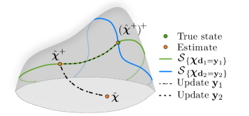
Figure 4: Graphical representation of two consecutive noise-free updates for an IIEKF. The filter is first updated with measurement $\mathbf{y}_{1}$, and then with measurement $\mathbf{y}_{2}$.

By contrast, a generic iterated EKF (on Lie groups), would probably fail to converge to the intersection in one cycle over the measurements. Indeed, even if we assume each GN update converges to the true minimum, ensuring the first updated estimate lies in the first subspace, then, when the second measurement is fed to the EKF, its estimate will step out of the first observed set, making the second update satisfy the second equation, but not the first anymore. This is illustrated in Fig. 5.

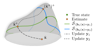
Figure 5: Graphical representation of two consecutive noise-free updates for a generic iterated EKF on Lie groups or manifolds. The filter is first updated with measurement $\mathbf{y}_{1}$, and then with measurement $\mathbf{y}_{2}$.

Remark 1.

When confronted with a system of equations in the right-invariant form, i.e., each of the form $\raisebox{1.0pt}{$\boldsymbol{\chi}$}^{-1}\mathbf{d}=\mathbf{y}$, we may rewrite them as $\mathbf{d}=\raisebox{1.0pt}{$\boldsymbol{\chi}$}\mathbf{y}$, and the same applies.

6.3 Illustration on $SO(3)$

Albeit a simple example, it is pedagogical to illustrate the results on a problem involving rotation matrices. Consider (51), where $\raisebox{1.0pt}{$\boldsymbol{\chi}$}\in SO(3)$, and where $\mathbf{d}_{1},\mathbf{d}_{2}\in\mathbb{R}^{3}$ are noncolinear unitary vectors, and so are $\mathbf{y}_{1},\mathbf{y}_{2}$. Assume we start with $\hat{}\raisebox{1.0pt}{$\boldsymbol{\chi}$}\in SO(3)$ close enough to the solution and $\mathbf{P}$ invertible, and we feed the IIEKF with noise-free measurement $\raisebox{1.0pt}{$\boldsymbol{\chi}$}\mathbf{d}_{1}=\mathbf{y}_{1}$. The IIEKF will output an estimate $\hat{}\raisebox{1.0pt}{$\boldsymbol{\chi}$}^{+}$ which satisfies $\hat{}\raisebox{1.0pt}{$\boldsymbol{\chi}$}^{+}\mathbf{d}_{1}=\mathbf{y}_{1}$. Then, if we feed the IIEKF with noise-free measurement $\raisebox{1.0pt}{$\boldsymbol{\chi}$}\mathbf{d}_{2}=\mathbf{y}_{2}$, all the iterates $\raisebox{1.0pt}{$\boldsymbol{\chi}$}^{+}\exp_{SO(3)}(\boldsymbol{\xi}^{i})$ underlying the IIEKF will remain in the set defined by $\raisebox{1.0pt}{$\boldsymbol{\chi}$}\mathbf{d}_{1}=\mathbf{y}_{1}$, as guaranteed by Proposition 2. Provided the GN converges, they will converge to the solution of the system of equations $(\hat{}\raisebox{1.0pt}{$\boldsymbol{\chi}$}^{+})^{+}$. We may redo the calculations in this simple case, to gain some geometric insight.

Proposition 5.

Consider an IIEKF with $\raisebox{1.0pt}{$\boldsymbol{\chi}$}\in SO(3)$ and full-rank initial covariance matrix. Assume it is fed with measurement $\raisebox{1.0pt}{$\boldsymbol{\chi}$}\mathbf{d}_{1}=\mathbf{y}_{1}$, and that the GN manages to converge, so that $\hat{}\raisebox{1.0pt}{$\boldsymbol{\chi}$}^{+}\mathbf{d}_{1}=\mathbf{y}_{1}$. Then, all immediate subsequent updates (or iterates) of the IIEKF consist of 2D rotations around the fixed axis $\mathbf{d}_{1}$, composed with the particular rotation $\hat{}\raisebox{1.0pt}{$\boldsymbol{\chi}$}^{+}$.

Proof.

This is direct consequence of (49). Indeed, in the present case $\exp_{SO(3)}(\boldsymbol{\delta})\mathbf{d}_{1}\approx\mathbf{d}_{1}+\mathbf{H}_{1}\boldsymbol{\delta}$ and furthermore from the definition of the exponential $\exp_{SO(3)}(\boldsymbol{\delta})\mathbf{d}_{1}\approx\mathbf{d}_{1}+\boldsymbol{\delta}\times\mathbf{d}_{1}$, so that $\mathbf{H}_{1}\boldsymbol{\delta}=\boldsymbol{\delta}\times\mathbf{d}_{1}$. The Riccati update ensures $\mathbf{H}_{1}\mathbf{P}^{+}\mathbf{H}_{1}^{T}=\mathbf{0}$, see Prop. 1, and the iterates are of the form $\hat{}\raisebox{1.0pt}{$\boldsymbol{\chi}$}^{i}=\hat{}\raisebox{1.0pt}{$\boldsymbol{\chi}$}^{+}\exp_{SO(3)}(\boldsymbol{\xi}^{i})$, with $\boldsymbol{\xi}^{i}\in\operatorname{Im}\mathbf{P}^{+}$, see (35). Thus $\mathbf{H}_{1}\boldsymbol{\xi}^{i}=\mathbf{0}$ and thus $\boldsymbol{\xi}^{i}\times\mathbf{d}_{1}=\mathbf{0}$. This immediately proves that $\exp_{SO(3)}(\boldsymbol{\xi}^{i})$ is a 2D rotation around $\mathbf{d}_{1}$, as $\exp_{SO(3)}(\boldsymbol{\xi}^{i})\mathbf{d}_{1}=\sum_{k\geq 0}[(\boldsymbol{\xi}^{i})]_{\times}^{k}\mathbf{d}_{1}=\mathbf{d}_{1}+\sum_{k\geq 1}[(\boldsymbol{\xi}^{i})]_{\times}^{k-1}(\boldsymbol{\xi}\times\mathbf{d}_{1})=\mathbf{d}_{1}+\mathbf{0}.$ ∎

This means that as soon as the first measurement is made, the IIEKF “focuses” on a problem of reduced dimension, namely seeking planar rotations in a 2D space. This makes it much more efficient as 1) it performs updates directly in a reduced subspace where the state is, and 2) it avoids destroying the information contained in the first measurement. The way noise-free measurements inherently remove degrees of freedom one by one in the estimation problem for the IIEKF certainly explains its fast convergence in the numerical experiments of the next section, although on a different problem.

7 Application of engineering interest

It is technically very feasible nowadays to mount an inertial measurement unit (IMU) on the hook of a crane that transmits its sensor readings [37], see illustration of Fig. 6. Estimating the position and velocity of the load from the IMU measurements may open the door to new automation capabilities since it allows for feedback, and may also increase safety [38]. However, the underlying dynamical model is unknown, as the hook does not necessarily follow a simple pendulum motion, because of external forces like friction and wind. The IMU dynamics, though, consist of kinematic relations which are satisfied at all times, whatever the motion. Moreover, when the cable is hanging, the distance between the hook and the cable hang-up point is the cable length, which is very accurately measured in modern cranes for safety reasons, see, e.g., [38]. We will use this as a very accurate–virtually perfect–measurement to gain information on the position of the hook.

We propose to compare in simulations the EKF, the iterated EKF (IterEKF) [3], the IEKF, and the proposed IIEKF on this estimation problem.

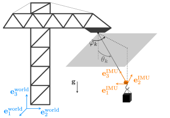
Figure 6: Crane with a wireless IMU mounted on its hook.

7.1 Dynamical system

Since they are rigidly attached, we assume the hook and the IMU share the same body frame. The state of the IMU, i.e., its “extended pose”, see [39], consists of: the rotation matrix $\mathbf{R}_{k}\in SO(3)$ from the IMU to the world frame, the IMU velocity vector $\mathbf{v}_{k}\in\mathbb{R}^{3}$ expressed in the world frame, and the IMU position vector $\mathbf{p}_{k}\in\mathbb{R}^{3}$ expressed in the world frame. In this paper, the EKF and IterEKF estimate the state

$$\mathbf{x}_{k}=(\mathbf{R}_{k},\mathbf{v}_{k},\mathbf{p}_{k})\in SO(3)\times\mathbb{R}^{3}\times\mathbb{R}^{3},$$ (52)

and use the estimation error defined as

$$\mathbf{e}_{k}=\begin{bmatrix}\log_{SO(3)}(\hat{\mathbf{R}}_{k}^{-1}\mathbf{R}_{k})\\ \mathbf{v}_{k}-\hat{\mathbf{v}}_{k}\\ \mathbf{p}_{k}-\hat{\mathbf{p}}_{k}\end{bmatrix},$$ (53)

where $\log_{SO(3)}:SO(3)\rightarrow\mathbb{R}^{3}$ is the logarithm map of group $SO(3)$. Similarly, we denote by $\mathbf{e}_{k}^{+}$ the error achieved by the updated estimate $\hat{\mathbf{x}}_{k}^{+}$. The IEKF and IIEKF estimate the state

$$\raisebox{1.0pt}{$\boldsymbol{\chi}$}_{k}=\begin{bmatrix}\mathbf{R}_{k}&\mathbf{v}_{k}&\mathbf{p}_{k}\\ \mathbf{0}&1&0\\ \mathbf{0}&0&1\end{bmatrix}\in SE_{2}(3),$$ (54)

where $SE_{2}(3)$ is the group of extended poses introduced in [13], see also [39]. Since measurements are expressed in the world frame, we use the left-invariant formalism, so that

$$\boldsymbol{\xi}_{k}:=\log_{SE_{2}(3)}(\hat{\raisebox{1.0pt}{$\boldsymbol{\chi}$}}_{k}^{-1}\raisebox{1.0pt}{$\boldsymbol{\chi}$}_{k}),\\$$ (55)

where $\log_{SE_{2}(3)}:SE_{2}(3)\rightarrow\mathbb{R}^{9}$ denotes the logarithm map of group $SE_{2}(3)$, see [14].

Without any prior knowledge about the motion, the dynamics of an IMU on flat Earth write

$$\mathbf{R}_{k+1} =\mathbf{R}_{k}\exp_{SO(3)}\left((\boldsymbol{\omega}_{k}+\mathbf{w}_{k}^{\boldsymbol{\omega}})dt\right),$$ (56a)

$$\mathbf{v}_{k+1} =\mathbf{v}_{k}+\left(\mathbf{R}_{k}(\mathbf{a}_{k}+\mathbf{w}_{k}^{\mathbf{a}})+\mathbf{g}\right)dt,$$ (56b)

$$\mathbf{p}_{k+1} =\mathbf{p}_{k}+\mathbf{v}_{k}dt,$$ (56c)

where the model inputs $\boldsymbol{\omega}_{k},\,\mathbf{a}_{k}\in\mathbb{R}^{3}$ are the angular velocity and the linear acceleration recorded by the IMU. They are both affected by normal noise $(\mathbf{w}^{\boldsymbol{\omega}}_{k},\mathbf{w}^{\mathbf{a}}_{k})\sim\mathcal{N}(\mathbf{0},\mathbf{Q})$ and are assumed to be free of any bias. Vector $\mathbf{g}=(0,0,-9.81)$ is the gravity vector expressed in the world frame and $dt$ is the integration time step. As shown in [13], the dynamics (56) are group affine, see [26] in discrete time. The Jacobians of the dynamics for each filter are available in Appendix C.3.

7.2 Measurements

The measurement $\mathbf{y}_{k}$ is the position of the hang-up point of the crane cable expressed in the world frame. It can be modeled using the function

$$\mathbf{y}_{k}=\mathbf{R}_{k}\mathbf{r}_{k}+\mathbf{p}_{k}+\mathbf{n}_{k},$$ (57)

where $\mathbf{r}_{k}=(0,0,l_{k})$ and $\mathbf{n}_{k}\sim\mathcal{N}(\mathbf{0},\mathbf{N})$. This model assumes the cable length $l_{k}$ to be known as well as the position $\mathbf{y}_{k}$. In modern cranes, they are both accurately measured via the encoders of the three motors of the crane [38]. The low noise inherent to those measurements is encapsulated within vector $\mathbf{n}_{k}$.

In the left-invariant framework, the model (57) writes

$$\begin{bmatrix}\mathbf{y}_{k}\\ 0\\ 1\end{bmatrix}=\raisebox{1.0pt}{$\boldsymbol{\chi}$}_{k}\mathbf{d}_{k}+\begin{bmatrix}\mathbf{n}_{k}\\ 0\\ 0\end{bmatrix},$$ (58)

where $\mathbf{d}_{k}=(0,0,l_{k},0,1)$ and with $\raisebox{1.0pt}{$\boldsymbol{\chi}$}_{k}$ as in (54). Note that the last two rows do not bring any useful information so that it is equivalent to (57). The Jacobians of the measurement function for each filter are available in Appendix C.3.

7.3 Simulations

We consider three different scenarios. It is important to note that in all of them, process noise is present and non-negligible. For each of them, we run $N_{\mathrm{s}}=200$ simulations in which the initial error is drawn randomly from the initial distribution. The performances are assessed by comparing the mean invariant error norm, that is,

$$E\left(\|\boldsymbol{\xi}_{k}^{+}\|\right)=\frac{1}{N_{\mathrm{s}}}\sum\limits_{n=1}^{N_{\mathrm{s}}}\left\|\log_{SE_{2}(3)}\left((\hat{\raisebox{1.0pt}{$\boldsymbol{\chi}$}}_{k,n}^{+})^{-1}\raisebox{1.0pt}{$\boldsymbol{\chi}$}_{k}\right)\right\|,$$ (59)

where $\hat{\raisebox{1.0pt}{$\boldsymbol{\chi}$}}_{k,n}^{+}$ is the updated estimate at time index $k$ in the $n^{\mathrm{th}}$ simulation. The three different scenarios are as follows.

7.3.1 Scenario 1

The ground-truth simulation corresponds to the trajectory followed by the hook with initial configuration:

$$\begin{split}\varphi_{0}=0\;$\mathrm{rad}$,\quad&\quad\theta_{0}=\frac{\pi}{4}\;$\mathrm{rad}$,\\ \dot{\varphi}_{0}=1\;$\mathrm{rad}\mathrm{/}\mathrm{s}$,\quad&\quad\dot{\theta}_{0}=0\;$\mathrm{rad}\mathrm{/}\mathrm{s}$,\end{split}$$ (60)

where $\varphi_{k}$ and $\theta_{k}$ are the azimuth and polar angles, see Fig. 6. No other external force than gravity is applied to the system. It is important to note that, in this configuration, the system is not observable, as shown in Appendix C.1. In addition to the average invariant error norm, we compute the average normalized estimation error squared (ANEES), denoted $\bar{\epsilon}_{k}$, in order to assess the consistency between the estimation error and the associated covariance matrix, see Appendix C.2 for more details. The trajectory of the hook is simulated for a total duration of $2.5\text{\,}\mathrm{s}$. The length of the cable follows the profile shown in Fig. 7.

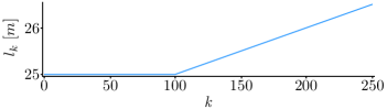
Figure 7: Evolution of the length of the crane cable $l_{k}$ as a function of the time index, used in simulations.

The IMU and estimation filters operate at the same frequency of $100\text{\,}\mathrm{Hz}$. The maximum number of iteration of the IterEKF and IIEKF is set to $N_{\mathrm{max}}=50$. The gyroscope and accelerometer are assumed to be consumer-grade devices, respectively with a standard deviation of $0.017\text{\,}\mathrm{rad}\mathrm{/}\mathrm{s}$ and $0.1\text{\,}\mathrm{m}\mathrm{/}\mathrm{s}\mathrm{{}^{2}}$ along each axis, giving the covariance matrix

$$\mathbf{Q}=\begin{bmatrix}(0.017)^{2}\mathbf{I}&\mathbf{0}\\ \mathbf{0}&(0.1)^{2}\mathbf{I}\end{bmatrix}.$$ (61)

The measurement noise is assumed to have a standard deviation of $1\text{\,}\mathrm{m}$ in every direction, giving $\mathbf{N}=\mathbf{I}.$

For a given simulation, all filters are initialized with the same initial estimation error. From one simulation to the next, the initial estimation error is randomly drawn from the initial distribution $\mathcal{N}(\mathbf{0},\mathbf{P}_{0})$ with

$$\mathbf{P}_{0}=\begin{bmatrix}(\frac{\pi}{6})^{2}\mathbf{I}&\mathbf{0}&\mathbf{0}\\ \mathbf{0}&(10)^{2}\mathbf{I}&\mathbf{0}\\ \mathbf{0}&\mathbf{0}&(10)^{2}\mathbf{I}\end{bmatrix}.$$ (62)

The tolerance for the convergence of iterative algorithms is set to $\mathrm{tol}=10^{-7}$.

7.3.2 Scenario 2 (restriction to 2D)

In this scenario, we assume the ground-truth trajectory is the trajectory followed by the hook having the following initial configuration:

$$\begin{split}\varphi_{0}=0\;$\mathrm{rad}$,\quad&\quad\theta_{0}=\frac{\pi}{4}\;$\mathrm{rad}$,\\ \dot{\varphi}_{0}=0\;$\mathrm{rad}\mathrm{/}\mathrm{s}$,\quad&\quad\dot{\theta}_{0}=0\;$\mathrm{rad}\mathrm{/}\mathrm{s}$.\end{split}$$ (63)

We also assume that the gyroscope variance along the first and third axes is null, as well as the accelerometer variance along the second axis. In this way, the motion of the hook is contained within the plane $\varphi_{k}=0$. In order to make the problem fully observable, we completely remove the uncertainty for rotations around the first and third axes, and for velocity and position around the second axis. All other parameters are kept identical to scenario 1.

7.3.3 Scenario 3 (restriction to 2D + noise-free measurements)

We now assume that the position of the cable hung-up point and the cable length are so accurately measured we may set $\mathbf{N}=\mathbf{0}$. All other parameters are kept identical to scenario 2. The system is therefore fully observable and measurements are noise-free. In accordance with the recommendations of Subsection 3.1, a regularized gain $\mathbf{K}_{k}^{\mathrm{rg}}=\mathbf{P}_{k}\mathbf{H}_{k}^{T}(\mathbf{H}_{k}\mathbf{P}_{k}\mathbf{H}_{k}^{T}+\delta\mathbf{I})^{-1}$ is used for all filters, with $\delta=10^{-5}$.

7.4 Results

Table 1 gathers the mean number of iterations needed for the GN method to converge in the update step of the IterEKF and IIEKF. In all three scenarios, the IIEKF requires less iterations. The biggest drop occurs in the third scenario, as could be anticipated from the insights of Section 6.3.

	Scenario 1	Scenario 2	Scenario 3
IterEKF	$8.03$	$6.1$	$8.1$
IIEKF	$\mathbf{6.2}$	$\mathbf{4.75}$	$\mathbf{3.15}$

Table 1: Mean number of Gauss-Newton iterations needed by the IterEKF and IIEKF to converge in each scenario. The smallest number is highlighted in bold for each scenario.

7.4.1 Scenario 1

The mean and standard deviation of the estimation error norm of each filter are displayed in graph (a) of Fig. 8. As expected for an unobservable system, the estimation error is lower bounded. The invariant methods outperform the EKF and IterEKF. A first factor contributing to this difference is the dependence on the state of the Jacobians used by the latter filters. When the estimate deviates significantly from the true trajectory, the Jacobians computed in such instances may differ completely from those calculated along the actual trajectory, leading to poor linearizations of the dynamics and output function.

A second factor is the problem of false observability inherent to the EKF: linearizing the output function (57) around the estimated trajectory may introduce spurious information that makes the system look observable. Graphs (b) and (c) of Fig. 8 show the evolution of the ANEES over time, which measures the ability of the filter to convey the actual extent of uncertainty associated to its estimates, see Appendix C.2 (the target value of the ANEES in the present example is 9). The EKF and IterEKF are overconfident about their estimation and their ANEES diverges. The IIEKF achieves an ANEES that almost entirely lies within the $95\%$-interval represented by the two horizontal dashed lines. This means it provides covariance matrices that are perfectly consistent with its estimation error, even in the transient. The IEKF initially under-estimates the estimation error before slowly recovering.

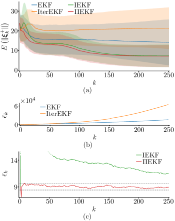
Figure 8: Results for scenario 1 (3D unobservable setting with process and measurement noises). (a) Mean and standard deviation (light color) of the estimation error norm as a function of the time index, computed over $200$ simulations. (b) Evolution of the ANEES as a function of the time index over $200$ simulations for the EKF and IterEKF. (c) Evolution of the ANEES as a function of the time index over $200$ simulations for the IEKF and IIEKF. The theoretical value of the ANEES is $N_{\mathrm{dof}}=9$. The two dashed horizontal lines delimit a $95\%$-confidence interval for the ANEES.

7.4.2 Scenario 2

The motion is now two-dimensional, so that the system is observable and the EKF and IterEKF do not suffer from false observability issues anymore. Fig. 9 shows that the IterEKF performs better than the EKF on average, with a smaller averaged error and a smaller variance across simulations. As in the previous scenario, the IEKF averaged error norm peaks after few time steps, before decreasing rapidly. The IIEKF exhibits the best performance: its estimation error is the smallest on average and presents the smallest variance across simulations. The IEKF and IIEKF have a much better convergence rate than the EKF and IterEKF. This is probably a direct consequence of the autonomy of their Jacobians w.r.t. the followed trajectory.

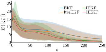
Figure 9: Results for scenario 2 (2D observable setting with noise). Mean and standard deviation (light color) of the estimation error norm as a function of the time index, computed over $200$ simulations.

7.4.3 Scenario 3

The measurements are now assumed to be noise-free and all four filters use the regularized gain (15) with $\delta=10^{-5}$. The mean and standard deviation of the estimation error norm are displayed in Fig. 10. Surprisingly, the IEKF is unstable when the measurement noise is too low and diverges. As the IEKF, the EKF is not well-suited to handling noise-free measurements: its averaged error norm presents a high transient variation before decreasing with a low convergence rate. During the first time steps, both iterative filters achieve a significant drop in their averaged estimation error norm. Then, the estimation error of the IIEKF quickly drops to a value close to $\mathbf{0}$ with almost no variance across simulations, while the error of the IterEKF slowly decreases towards zero with a relatively large variance across simulations. This scenario proves once more the superiority of the proposed IIEKF, and illustrates the theorems.

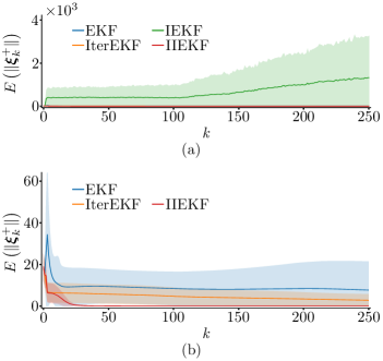
Figure 10: Results for scenario 3 (2D observable setting with process noise but noise-free measurements). (a) Mean and standard deviation (light color) of the estimation error norm as a function of the time index, computed over $200$ simulations. (b) Same as (a) where the IEKF is removed.

8 Conclusion

In this paper, we introduced the iterated invariant EKF. Its features and advantages, when applied to systems on Lie groups with left-invariant measurements, are as follows.

• In the absence of measurement noise, the IIEKF “hard codes” the measurement, inherently removing one degree of freedom in the estimation problem, making (immediate) subsequent updates more efficient.

• In the presence of low measurement noise, as there is a continuum between the noise-free and noisy case, this indicates the IIEKF incorporates the measurement by making the estimate land within a subspace where the state is very likely to be, and then performs updates that remain within (or close to) this subspace. This must explain its speed of convergence in the simulations.

• In the general case, whatever the level of noise, the IIEKF is anyway an improvement over the IEKF, which has been shown to be very well behaved in numerous applications. Indeed, the IIEKF leaves the IEKF’s Riccati update untouched, while refining its state estimate (the IEKF being exactly an IIEKF with one iteration).

In numerical experiments, the IIEKF showed unmatched performances in all presented scenarios while consistently estimating the error covariance. It was also shown to apply to the “novel” problem of solving a system of equations of the form $\raisebox{1.0pt}{$\boldsymbol{\chi}$}\mathbf{d}=\mathbf{y}$ on a matrix Lie group.

In terms of limitations, the IIEKF is reserved for systems with invariant measurements. However, note that the class of measurements possessing the required invariant property is large, and has recently been further extended in [26].

As a perspective, we would like to apply this iterative estimation technique to further problems where the IEKF proved successful, notably highly accurate navigation. We would also like to bring the IIEKF to bear on problems of state estimation with constraints, where constraints could be enforced by using them as pseudo-measurements, as was done in the subgroup intersection problem.

Appendix A Consistency of the linear Kalman filter when facing noise-free measurements

Theorem 3.

Consider the linear noise-free measurement

$$\mathbf{y}_{k}=\mathbf{H}_{k}\mathbf{x}_{k}.$$ (64)

Let $\mathbf{K}_{k}^{\mathrm{nf}}=\mathbf{L}_{k}(\mathbf{H}_{k}\mathbf{L}_{k})^{\dagger}$ be the Kalman gain in the limit case of noise-free measurement developed in our preliminary paper [30], with $\mathbf{P}_{k}=\mathbf{L}_{k}\mathbf{L}_{k}^{T}$. The Kalman update, defined as (3d)-(3e) but replacing the gain $\mathbf{K}_{k}$ with $\mathbf{K}_{k}^{\mathrm{nf}}$, satisfies Property 1, that is, $\mathbf{H}_{k}\hat{\mathbf{x}}_{k}^{+}=\mathbf{y}_{k}$ and $\mathbf{H}_{k}\mathbf{P}_{k}^{+}\mathbf{H}_{k}=\mathbf{0}$.

Proof.

Using (3d), it comes

$$\mathbf{H}_{k}\hat{\mathbf{x}}_{k}^{+} =\mathbf{H}_{k}\hat{\mathbf{x}}_{k}+\mathbf{H}_{k}\mathbf{K}_{k}^{\mathrm{nf}}\mathbf{z}_{k},$$ (65a)

$$=\mathbf{y}_{k}-\mathbf{z}_{k}+\mathbf{H}_{k}\mathbf{K}_{k}^{\mathrm{nf}}\mathbf{z}_{k},$$ (65b)

$$=\mathbf{y}_{k}+(\mathbf{H}_{k}\mathbf{K}_{k}^{\mathrm{nf}}-\mathbf{I})\mathbf{z}_{k},$$ (65c)

$$=\mathbf{y}_{k}+(\mathbf{H}_{k}\mathbf{K}_{k}^{\mathrm{nf}}\mathbf{H}_{k}-\mathbf{H}_{k})(\mathbf{x}_{k}-\hat{\mathbf{x}}_{k}).$$ (65d)

The estimation error $(\mathbf{x}_{k}-\hat{\mathbf{x}}_{k})$ follows the distribution $\mathcal{N}(\mathbf{0},\mathbf{L}_{k}\mathbf{L}_{k}^{T})$. Consequently, there always exists a vector $\mathbf{v}$ such that $(\mathbf{x}_{k}-\hat{\mathbf{x}}_{k})=\mathbf{L}_{k}\mathbf{v}$. Noting that $\mathbf{K}_{k}^{\mathrm{nf}}=\mathbf{L}_{k}(\mathbf{H}_{k}\mathbf{L}_{k})^{\dagger}$ and using the property of the pseudo-inverse $\mathbf{A}\mathbf{A}^{\dagger}\mathbf{A}=\mathbf{A}$, yields

$$\mathbf{H}_{k}\hat{\mathbf{x}}_{k}^{+} =\mathbf{y}_{k}+(\mathbf{H}_{k}\mathbf{L}_{k}(\mathbf{H}_{k}\mathbf{L}_{k})^{\dagger}\mathbf{H}_{k}\mathbf{L}_{k}-\mathbf{H}_{k}\mathbf{L}_{k})\mathbf{v},$$ (66a)

$$=\mathbf{y}_{k}+(\mathbf{H}_{k}\mathbf{L}_{k}-\mathbf{H}_{k}\mathbf{L}_{k})\mathbf{v}=\mathbf{y}_{k}.$$ (66b)

Then, using (3e) and $\mathbf{K}_{k}^{\mathrm{nf}}=\mathbf{L}_{k}(\mathbf{H}_{k}\mathbf{L}_{k})^{\dagger}$, it comes

$$\mathbf{H}_{k}\mathbf{P}_{k}^{+}\mathbf{H}_{k}^{T} =(\mathbf{H}_{k}-\mathbf{H}_{k}\mathbf{L}_{k}(\mathbf{H}_{k}\mathbf{L}_{k})^{\dagger}\mathbf{H}_{k})\mathbf{P}_{k}\mathbf{H}_{k}^{T},$$ (67a)

$$=(\mathbf{H}_{k}-\mathbf{H}_{k}\mathbf{L}_{k}(\mathbf{H}_{k}\mathbf{L}_{k})^{\dagger}\mathbf{H}_{k})\mathbf{L}_{k}\mathbf{L}_{k}^{T}\mathbf{H}_{k}^{T},$$ (67b)

$$=(\mathbf{H}_{k}\mathbf{L}_{k}-\mathbf{H}_{k}\mathbf{L}_{k}(\mathbf{H}_{k}\mathbf{L}_{k})^{\dagger}\mathbf{H}_{k}\mathbf{L}_{k})\mathbf{L}_{k}^{T}\mathbf{H}_{k}^{T},$$ (67c)

$$=(\mathbf{H}_{k}\mathbf{L}_{k}-\mathbf{H}_{k}\mathbf{L}_{k})\mathbf{L}_{k}^{T}\mathbf{H}_{k}^{T}=\mathbf{0}.$$ (67d)

∎

Theorem 4.

Let $(\hat{\mathbf{x}}_{k},\mathbf{P}_{k})$ be the belief of a Kalman filter that is compatible with the measurement $\mathbf{y}_{k}=\mathbf{H}_{k}\mathbf{x}_{k}$ in the sense of Definition 2. Consider a different (possibly noisy) measurement $\tilde{\mathbf{y}}_{k}=\tilde{\mathbf{H}}_{k}\mathbf{x}_{k}+\mathbf{n}_{k}$. The updated belief $(\hat{\mathbf{x}}_{k}^{+},\mathbf{P}_{k}^{+})$ in the light of measurement $\tilde{\mathbf{y}}_{k}$ remains compatible with measurement $\mathbf{y}_{k}$ in the sense of Definition 2, i.e., the Kalman filter satisfies Property 2.

Proof.

Let $\tilde{\mathbf{K}}_{k}$ and $\tilde{\mathbf{z}}_{k}$ be the Kalman gain and the innovation associated to measurement $\tilde{\mathbf{y}}_{k}$. Let $\operatorname{Im}{\mathbf{A}}$ and $\operatorname{Ker}\mathbf{A}$ respectively denote the image and kernel of matrix $\mathbf{A}$. The equality $\mathbf{H}_{k}\mathbf{P}_{k}\mathbf{H}_{k}^{T}=\mathbf{0}$ implies $\operatorname{Im}{\mathbf{P}_{k}}\subset\operatorname{Ker}\mathbf{H}_{k}$. By definition of the Kalman gain, we have

$$\operatorname{Im}\tilde{\mathbf{K}}_{k}\subseteq\operatorname{Im}\mathbf{P}_{k}\subset\operatorname{Ker}\mathbf{H}_{k},$$ (68)

in such a way that $\mathbf{H}_{k}\tilde{\mathbf{K}}_{k}=\mathbf{0}$. Consequently, $\mathbf{H}_{k}\hat{\mathbf{x}}_{k}^{+}=\mathbf{H}_{k}(\hat{\mathbf{x}}_{k}+\tilde{\mathbf{K}_{k}}\tilde{\mathbf{z}}_{k})=\mathbf{H}_{k}\hat{\mathbf{x}}_{k}+\mathbf{H}_{k}\tilde{\mathbf{K}_{k}}\tilde{\mathbf{z}}_{k}=\mathbf{H}_{k}\hat{\mathbf{x}}_{k}=\mathbf{y}_{k}.$ Similarly, we get $\mathbf{H}_{k}\mathbf{P}_{k}^{+}\mathbf{H}_{k}^{T}=(\mathbf{H}_{k}-\mathbf{H}_{k}\tilde{\mathbf{K}}_{k}\tilde{\mathbf{H}}_{k})\mathbf{P}_{k}\mathbf{H}_{k}^{T}=\mathbf{H}_{k}\mathbf{P}_{k}\mathbf{H}_{k}^{T}=\mathbf{0}.$ In the case $\tilde{\mathbf{y}}_{k}$ is a noise-free measurement and the noise-free gain $\mathbf{K}_{k}^{\mathrm{nf}}$ is used, the same result applies as $\operatorname{Im}\mathbf{K}_{k}^{\mathrm{nf}}\subseteq\operatorname{Im}\mathbf{P}_{k}$ too. ∎

Appendix B Right Lie Jacobian

The matrix $\mathbf{\mathcal{J}}_{r}(\boldsymbol{\xi})$ denotes the right Jacobian of group $G$ evaluated at $\boldsymbol{\xi}$, see [31]. It is defined through the relation

$$\mathcal{L}_{\mathfrak{g}}(\mathbf{\mathcal{J}}_{r}(\mathbf{a})^{-1}\mathbf{b})=\sum\limits_{n=0}^{+\infty}\frac{B_{n}}{n!}\underbrace{[\mathcal{L}_{\mathfrak{g}}(\mathbf{a}),[\mathcal{L}_{\mathfrak{g}}(\mathbf{a}),\dots[\mathcal{L}_{\mathfrak{g}}(\mathbf{a})}_{n},\mathcal{L}_{\mathfrak{g}}(\mathbf{b})]\dots]],$$ (69)

where $B_{n}$ are the Bernoulli numbers, $[\mathbf{A},\mathbf{B}]$ is the usual Lie bracket $\mathbf{A}\mathbf{B}-\mathbf{B}\mathbf{A}$, and $\mathcal{L}_{\mathfrak{g}}(\cdot):\mathbb{R}^{n}\rightarrow\mathfrak{g}$ is the bijective map between the Lie algebra $\mathfrak{g}$ of $G$ and the associated vector space, see $\mathbb{R}^{n}$ [40], defined by $\exp(\boldsymbol{\xi})\approx\mathbf{I}+\mathcal{L}_{\mathfrak{g}}(\boldsymbol{\xi})$ neglecting second-order terms in $\boldsymbol{\xi}$. Closed-form expressions for the right Jacobians of the groups $SO(3)$ and $SE(3)$ are provided in [40]. The right Jacobian of the group of extended pose $SE_{2}(3)$ is detailed in [39].

Appendix C Crane application: implementation details

C.1 Observability

Quite intuitively, the rotation around the gravity vector is not observable. Indeed, the sequence of IMU outputs produced by following a trajectory remains unchanged by any rotation of the initial state around the gravity vector. This makes it impossible to differentiate two trajectories starting from initial configurations that differ only in azimuth angle $\varphi_{0}$. This can be shown mathematically as followed. Considering no process and no measurement noise, the linearized error system from the invariant framework writes

$$\boldsymbol{\xi}_{k+1} =\mathbf{F}_{k}\boldsymbol{\xi}_{k},$$ (70a)

$$\mathbf{z}_{k} =\exp_{SE_{2}(3)}\left(\boldsymbol{\xi}_{k}\right)\mathbf{d}_{k}-\mathbf{d}_{k}.$$ (70b)

Due to the log-linearity property of the IEKF, see [26], observability can be assessed using system (70). For this system to be observable, we must be able to retrieve $\boldsymbol{\xi}_{k}$ from past inputs and past innovations. Since $\mathbf{z}_{k}$ is a nonlinear function of $\boldsymbol{\xi}_{k}$, observability can only be assessed locally. Up to the first order, we get

$$\begin{bmatrix}\mathbf{z}_{k}\\ \mathbf{z}_{k-1}\\ \mathbf{z}_{k-2}\end{bmatrix} =\begin{bmatrix}\exp_{SE_{2}(3)}\left(\boldsymbol{\xi}_{k}\right)\mathbf{d}_{k}-\mathbf{d}_{k}\\ \exp_{SE_{2}(3)}\left(\mathbf{F}_{k-1}^{-1}\boldsymbol{\xi}_{k}\right)\mathbf{d}_{k-1}-\mathbf{d}_{k-1}\\ \exp_{SE_{2}(3)}\left(\mathbf{F}_{k-2}^{-1}\mathbf{F}_{k-1}^{-1}\boldsymbol{\xi}_{k}\right)\mathbf{d}_{k-2}-\mathbf{d}_{k-2}\end{bmatrix},$$ (71a)

$$\approx\begin{bmatrix}\mathbf{H}_{k}\\ \mathbf{H}_{k-1}\mathbf{F}_{k-1}^{-1}\\ \mathbf{H}_{k-2}\mathbf{F}_{k-2}^{-1}\mathbf{F}_{k-1}^{-1}\end{bmatrix}\boldsymbol{\xi}_{k}$$ (71b)

$$\approx\underbrace{\begin{bmatrix}-(\mathbf{r}_{k})_{\times}&\mathbf{0}&\mathbf{I}\\ \boldsymbol{\Psi}&-dt\boldsymbol{\Omega}_{k-1}&\boldsymbol{\Omega}_{k-1}\\ \boldsymbol{\Sigma}&-2dt\boldsymbol{\Phi}&\boldsymbol{\Phi}\end{bmatrix}}_{\mathcal{O}}\boldsymbol{\xi}_{k},$$ (71c)

where $\mathcal{O}$ is the observability matrix with

$$\boldsymbol{\Psi} =-(\mathbf{r}_{k-1}+dt^{2}\mathbf{a}_{k-1})_{\times}\boldsymbol{\Omega}_{k-1},$$ (72a)

$$\boldsymbol{\Phi} =\boldsymbol{\Omega}_{k-2}\boldsymbol{\Omega}_{k-1},$$ (72b)

$$\boldsymbol{\Sigma} =-\boldsymbol{\Phi}(\boldsymbol{\Phi}^{-1}(\mathbf{r}_{k-2}+dt^{2}\mathbf{a}_{k-2})+2dt^{2}\boldsymbol{\Omega}_{k-1}^{-1}\mathbf{a}_{k-1})_{\times},$$ (72c)

where $\boldsymbol{\Omega}_{k}=\exp_{SO(3)}(\omega_{k}dt)$ and $(\cdot)_{\times}:\mathbb{R}^{3}\rightarrow\mathfrak{so}(3)$ is the skew-symmetric operator associated to cross product on $\mathbb{R}^{3}$. The six first rows of matrix $\mathcal{O}$ are linearly independent. Denoting by $\mathbf{O}_{i}\in\mathbb{R}^{3\times 9}$ the $i^{\mathrm{th}}$ $3\times 9$ block-row of matrix $\mathcal{O}$, and performing the linear combination

$$\mathbf{O}_{3}\leftarrow-\boldsymbol{\Phi}^{-1}\mathbf{O}_{3}+2\boldsymbol{\Omega}_{k-1}^{-1}\mathbf{O}_{2}-\mathbf{O}_{1},$$ (73)

it comes

$$\mathbf{O}_{3}=\begin{bmatrix}(\boldsymbol{\Phi}^{-1}(\mathbf{r}_{k-2}+dt^{2}\mathbf{a}_{k-2})-2\boldsymbol{\Omega}_{k-1}^{-1}\mathbf{r}_{k-1}+\mathbf{r}_{k})_{\times}&\mathbf{0}\end{bmatrix}.$$ (74)

The rank of $\mathbf{O}_{3}$ is either $2$ or $0$ as the skew-symmetric matrix $(\mathbf{b})_{\times}$ has a rank equal to $2$ whenever $\mathbf{b}$ is not $\mathbf{0}$. System (70) is therefore not observable as the observability matrix $\mathcal{O}$ is not full rank.

C.2 Average normalized estimation error squared (ANEES)

The ANEES is defined by

$$\bar{\epsilon}_{k}=\frac{1}{N_{\mathrm{s}}}\sum\limits_{n=1}^{N_{\mathrm{s}}}\mathbf{e}_{k,n}^{+T}(\mathbf{P}_{k}^{+})^{-1}\mathbf{e}_{k,n}^{+},$$ (75)

for the EKF and IterEKF, and by

$$\bar{\epsilon}_{k}=\frac{1}{N_{\mathrm{s}}}\sum\limits_{n=1}^{N_{\mathrm{s}}}\boldsymbol{\xi}_{k,n}^{+T}(\mathbf{P}_{k,n}^{+})^{-1}\boldsymbol{\xi}_{k,n}^{+},$$ (76)

for the IEKF and IIEKF. The subscript $n$ is the index of the current simulation among the $N_{s}$ simulations. Let $N_{\mathrm{dof}}$ be the number of freedom degrees of the considered motion. The ANEES converges towards $N_{\mathrm{dof}}$ and the random variable $N_{\mathrm{s}}\bar{\epsilon}_{k}$ follows a Chi-Square distribution with $N_{\mathrm{s}}N_{\mathrm{dof}}$ degrees of freedom. A $95\%$-confidence interval $[r_{1},r_{2}]$ for $\bar{\epsilon}_{k}$ can be computed, where

$$r_{1}=\frac{1}{N_{\mathrm{s}}}F^{-1}_{\chi^{2}_{N_{\mathrm{s}}N_{\mathrm{dof}}}}(0.025),$$ (77)

and

$$r_{2}=\frac{1}{N_{\mathrm{s}}}F^{-1}_{\chi^{2}_{N_{\mathrm{s}}N_{\mathrm{dof}}}}(0.975),$$ (78)

with $F^{-1}_{\chi^{2}_{N_{\mathrm{s}}N_{\mathrm{dof}}}}$ the inverse cumulative distribution function of the Chi-Square distribution. An ANEES above $r_{2}$ is the sign of an over-confident filter, while an ANEES below $r_{1}$ characterizes an under-confident filter.

C.3 Jacobians

The dynamics and output Jacobians of the EKF and IterEKF are given by

$$\mathbf{F}_{k}^{\mathrm{EKF}}=\begin{bmatrix}\boldsymbol{\Omega}_{k}^{-1}&\mathbf{0}&\mathbf{0}\\ -\hat{\mathbf{R}}_{k}(\mathbf{a}_{k})_{\times}dt&\mathbf{I}&\mathbf{0}\\ \mathbf{0}&\mathbf{I}dt&\mathbf{I}\end{bmatrix},$$ (79)

and

$$\mathbf{H}_{k}^{\mathrm{EKF}}=\begin{bmatrix}-\hat{\mathbf{R}}_{k}(\mathbf{r}_{k})_{\times}&\mathbf{0}&\mathbf{I}\end{bmatrix},$$ (80)

where $(\cdot)_{\times}$ is the skew-symmetric operator associated with cross product in $\mathbb{R}^{3}$, and where $\boldsymbol{\Omega}_{k}=\exp_{SO(3)}(\boldsymbol{\omega}_{k}dt)$. The Jacobian of the dynamics w.r.t. the process noise is given by

$$\mathbf{G}_{k}^{\mathrm{EKF}}=\begin{bmatrix}\mathbf{J}_{l}(-\boldsymbol{\omega}_{k}dt)dt&\mathbf{0}\\ \mathbf{0}&\hat{\mathbf{R}}_{k}dt\\ \mathbf{0}&\mathbf{0}\end{bmatrix},$$ (81)

where $\mathbf{J}_{l}(-\boldsymbol{\omega}_{k}dt)$ is the left Jacobian of $SO(3)$ evaluated at $-\boldsymbol{\omega}_{k}dt$, see [40]. The recent two-frames theory [26] provides a clear and fast way to derive the dynamics and output Jacobians for the IEKF and IIEKF. For the problem at hand, the theory respectively yields, see Proposition 13 of [26],

$$\mathbf{F}_{k}^{\mathrm{IEKF}}=\begin{bmatrix}\boldsymbol{\Omega}_{k}^{-1}&\mathbf{0}&\mathbf{0}\\ -\,\boldsymbol{\Omega}_{k}^{-1}(\mathbf{a}_{k})_{\times}dt&\boldsymbol{\Omega}_{k}^{-1}&\mathbf{0}\\ \mathbf{0}&\boldsymbol{\Omega}_{k}^{-1}dt&\boldsymbol{\Omega}_{k}^{-1}\end{bmatrix},$$ (82)

and

$$\mathbf{H}_{k}^{\mathrm{IEKF}}=\begin{bmatrix}-(\mathbf{r}_{k})_{\times}&\mathbf{0}&\mathbf{I}\end{bmatrix}.$$ (83)

The Jacobian of the dynamics w.r.t. the process noise is given by

$$\mathbf{G}_{k}^{\mathrm{IEKF}}=\begin{bmatrix}\mathbf{J}_{l}(-\boldsymbol{\omega}_{k}dt)dt&\mathbf{0}\\ \mathbf{0}&\boldsymbol{\Omega}_{k}^{-1}dt\\ \mathbf{0}&\mathbf{0}\end{bmatrix}.$$ (84)

In the following, the superscripts EKF and IEKF are dropped when the context is clear enough.

Appendix D Difference with the iterated EKF on Lie groups

The IIEKF differs from the iterated EKF on Lie groups of [6] in various important respects, as [6] is concerned with adapting the iterated EKF to the manifold structure of the state space at a general level, whereas we pursue an approach tailored to a specific class of measurements. In particular the IIEKF boils down to the IEKF when using one iteration, which shows its specificity.

More in detail, the differences are: 1) We presented the IIEKF in the left-invariant formalism and assumed the state follows the concentrated Gaussian distribution (26), while [6] models uncertainty with the concentrated Gaussian defined through right multiplication, that is,

$$\raisebox{1.0pt}{$\boldsymbol{\chi}$}_{k}=\exp_{G}(\boldsymbol{\xi}_{k})\hat{\raisebox{1.0pt}{$\boldsymbol{\chi}$}}_{k},\quad\text{with $\boldsymbol{\xi}_{k}\sim\mathcal{N}(\mathbf{0},\mathbf{P}_{k})$}.$$ (85)

This is arbitrary anyway, as [6] makes no assumption regarding the output map, leading to a general algorithm, but without exploiting any relation between the uncertainty representation and the measurements, whereas in our work the relationship is very strong, as dramatically illustrated by Proposition 3. 2) We consider (left-)invariant measurements of the form (24b) and use the innovation defined by (28b). Our Jacobian $\mathbf{H}_{k}$ is therefore independent from the current estimate, see [14]. This autonomy w.r.t. the current estimate makes our Riccati update (39) completely independent from the outcome of the GN iterative scheme, contrary to [6]. 3) The work about EKF on Lie groups [41, 6] focuses on standard groups such as $SE(3)$ or direct products of the form $SO(3)\times\mathbb{R}^{k}$ and does not seek to exploit the relation between the dynamics, or the measurement map, and the group structure, that allows in particular to define interesting innovation variables. 4) We presented the MAP optimization problem as an optimization over the variable $\boldsymbol{\xi}$, see (31), so that the GN method is applied to a function whose domain is the vector space $\mathbb{R}^{n}$. By contrast, the LG-GN developed in [6], operates directly on the Lie group $G$. This requires the computation of additional Jacobians in the iterative scheme, see (53) in [6]. 5) We have derived strong theoretical guarantees for the IIEKF.

References

- [1] R. E. Kalman, “A new approach to linear filtering and prediction problems,” Transactions of the ASME–Journal of Basic Engineering, vol. 82, no. Series D, pp. 35–45, 1960.
- [2] S. F. Schmidt, “The kalman filter-its recognition and development for aerospace applications,” Journal of Guidance and Control, vol. 4, no. 1, pp. 4–7, 1981.
- [3] B. M. Bell and F. W. Cathey, “The iterated kalman filter update as a gauss-newton method,” IEEE Transactions on Automatic Control, vol. 38, no. 2, pp. 294–297, 1993.
- [4] J. Zhao, M. Netto, and L. Mili, “A robust iterated extended kalman filter for power system dynamic state estimation,” IEEE Transactions on Power Systems, vol. 32, no. 4, pp. 3205–3216, 2016.
- [5] M. Bloesch, M. Burri, S. Omari, M. Hutter, and R. Siegwart, “Iterated extended kalman filter based visual-inertial odometry using direct photometric feedback,” The International Journal of Robotics Research, vol. 36, no. 10, pp. 1053–1072, 2017.
- [6] G. Bourmaud, R. Mégret, A. Giremus, and Y. Berthoumieu, “From intrinsic optimization to iterated extended kalman filtering on lie groups,” Journal of Mathematical Imaging and Vision, vol. 55, pp. 284–303, 2016.
- [7] B. Liu, H. Chen, and W. Zhang, “A general iterative extended kalman filter framework for state estimation on matrix lie groups,” in 2023 62nd IEEE Conference on Decision and Control (CDC). IEEE, 2023, pp. 1177–1182.
- [8] N. van Der Laan, M. Cohen, J. Arsenault, and J. R. Forbes, “The invariant rauch-tung-striebel smoother,” IEEE Robotics and Automation Letters, vol. 5, no. 4, pp. 5067–5074, 2020.
- [9] L. Liang-Qun, J. Hong-Bing, and L. Jun-Hui, “The iterated extended kalman particle filter,” in IEEE International Symposium on Communications and Information Technology, 2005. ISCIT 2005., vol. 2. IEEE, 2005, pp. 1213–1216.
- [10] S. Bonnabel and P. Rouchon, “On invariant observers,” Control and observer design for nonlinear finite and infinite dimensional systems, pp. 53–65, 2005.
- [11] R. Mahony, T. Hamel, and J.-M. Pflimlin, “Nonlinear complementary filters on the special orthogonal group,” IEEE Transactions on automatic control, vol. 53, no. 5, pp. 1203–1218, 2008.
- [12] M. R. Cohen and J. R. Forbes, “Navigation and control of unconventional vtol uavs in forward-flight with explicit wind velocity estimation,” IEEE Robotics and Automation Letters, vol. 5, no. 2, pp. 1151–1158, 2020.
- [13] A. Barrau and S. Bonnabel, “The invariant extended kalman filter as a stable observer,” IEEE Transactions on Automatic Control, vol. 62, no. 4, pp. 1797–1812, 2016.
- [14] ——, “Invariant kalman filtering,” Annual Review of Control, Robotics, and Autonomous Systems, vol. 1, no. 1, pp. 237–257, 2018.
- [15] R. Mahony and T. Hamel, “A geometric nonlinear observer for simultaneous localisation and mapping,” in 2017 IEEE 56th Annual Conference on Decision and Control (CDC). IEEE, 2017, pp. 2408–2415.
- [16] P. van Goor, R. Mahony, T. Hamel, and J. Trumpf, “A geometric observer design for visual localisation and mapping,” in 2019 IEEE 58th Conference on Decision and Control (CDC). IEEE, 2019, pp. 2543–2549.
- [17] R. Mahony, T. Hamel, and J. Trumpf, “An homogeneous space geometry for simultaneous localisation and mapping,” Annual Reviews in Control, vol. 51, pp. 254–267, 2021.
- [18] R. Hartley, M. Ghaffari, R. M. Eustice, and J. W. Grizzle, “Contact-aided invariant extended kalman filtering for robot state estimation,” The International Journal of Robotics Research, vol. 39, no. 4, pp. 402–430, 2020.
- [19] N. Pavlasek, A. Walsh, and J. R. Forbes, “Invariant extended kalman filtering using two position receivers for extended pose estimation,” in 2021 IEEE International Conference on Robotics and Automation (ICRA). IEEE, 2021, pp. 5582–5588.
- [20] K. Wu, T. Zhang, D. Su, S. Huang, and G. Dissanayake, “An invariant-ekf vins algorithm for improving consistency,” in 2017 IEEE/RSJ International Conference on Intelligent Robots and Systems (IROS), Sep. 2017, pp. 1578–1585.
- [21] S. Heo and C. G. Park, “Consistent ekf-based visual-inertial odometry on matrix lie group,” IEEE Sensors Journal, vol. 18, no. 9, pp. 3780–3788, May 2018.
- [22] M. Wang and A. Tayebi, “Hybrid nonlinear observers for inertial navigation using landmark measurements,” IEEE Transactions on Automatic Control, vol. 65, no. 12, pp. 5173–5188, 2020.
- [23] H. A. Hashim, “Gps-denied navigation: Attitude, position, linear velocity, and gravity estimation with nonlinear stochastic observer,” in 2021 American Control Conference (ACC). IEEE, 2021, pp. 1149–1154.
- [24] P. van Goor and R. Mahony, “Autonomous error and constructive observer design for group affine systems,” in 2021 60th IEEE Conference on Decision and Control (CDC). IEEE, 2021, pp. 4730–4737.
- [25] A. Barrau, “Non-linear state error based extended kalman filters with applications to navigation,” Ph.D. dissertation, Mines Paristech, 2015.
- [26] A. Barrau and S. Bonnabel, “The geometry of navigation problems,” IEEE Transactions on Automatic Control, vol. 68, no. 2, pp. 689–704, 2023.
- [27] R. Mahony and J. Trumpf, “Equivariant filter design for kinematic systems on lie groups,” IFAC-PapersOnLine, vol. 54, no. 9, pp. 253–260, 2021.
- [28] C. C. Paige and M. A. Saunders, “Lsqr: An algorithm for sparse linear equations and sparse least squares,” ACM Transactions on Mathematical Software (TOMS), vol. 8, no. 1, pp. 43–71, 1982.
- [29] D. Simon and T. L. Chia, “Kalman filtering with state equality constraints,” IEEE transactions on Aerospace and Electronic Systems, vol. 38, no. 1, pp. 128–136, 2002.
- [30] S. Goffin, S. Bonnabel, O. Brüls, and P. Sacré, “Invariant kalman filtering with noise-free pseudo-measurements,” in 2023 62nd IEEE Conference on Decision and Control (CDC), 2023, pp. 8665–8671.
- [31] G. S. Chirikjian, Stochastic Models, Information Theory, and Lie Groups, Volume 1: Classical Results and Geometric Methods. Springer Science & Business Media, 2009.
- [32] Y. Wang and G. S. Chirikjian, “Error propagation on the euclidean group with applications to manipulator kinematics,” IEEE Transactions on Robotics, vol. 22, no. 4, pp. 591–602, 2006.
- [33] K. C. Wolfe, M. Mashner, and G. S. Chirikjian, “Bayesian fusion on lie groups,” Journal of Algebraic Statistics, vol. 2, no. 1, 2011.
- [34] G. Bourmaud, R. Mégret, M. Arnaudon, and A. Giremus, “Continuous-discrete extended kalman filter on matrix lie groups using concentrated gaussian distributions,” Journal of Mathematical Imaging and Vision, vol. 51, pp. 209–228, 2015.
- [35] P. Chauchat, A. Barrau, and S. Bonnabel, “Kalman filtering with a class of geometric state equality constraints,” in 2017 IEEE 56th Annual Conference on Decision and Control (CDC). IEEE, 2017, pp. 2581–2586.
- [36] A. Barrau and S. Bonnabel, “Extended kalman filtering with nonlinear equality constraints: a geometric approach,” IEEE Transactions on Automatic Control, vol. 65, no. 6, pp. 2325–2338, 2019.
- [37] F. Rauscher, S. Nann, and O. Sawodny, “Motion control of an overhead crane using a wireless hook mounted IMU,” in 2018 Annual American Control Conference (ACC). IEEE, 2018, pp. 5677–5682.
- [38] S. Bonnabel and X. Claeys, “The industrial control of tower cranes: An operator-in-the-loop approach [applications in control],” IEEE Control Systems Magazine, vol. 40, no. 5, pp. 27–39, 2020.
- [39] M. Brossard, A. Barrau, P. Chauchat, and S. Bonnabel, “Associating uncertainty to extended poses for on lie group imu preintegration with rotating earth,” IEEE Transactions on Robotics, vol. 38, no. 2, pp. 998–1015, 2021.
- [40] T. D. Barfoot, State estimation for robotics. Cambridge University Press, 2017.
- [41] G. Bourmaud, R. Mégret, A. Giremus, and Y. Berthoumieu, “Discrete extended kalman filter on lie groups,” in 21st European Signal Processing Conference (EUSIPCO 2013). IEEE, 2013, pp. 1–5.