Analytical Approximation of the ELBO Gradient
in the Context of the Clutter Problem
Abstract
We propose an analytical solution for approximating the gradient of the Evidence Lower Bound (ELBO) in variational inference problems where the statistical model is a Bayesian network consisting of observations drawn from a mixture of a Gaussian distribution embedded in unrelated clutter, known as the clutter problem. The method employs the reparameterization trick to move the gradient operator inside the expectation and relies on the assumption that, because the likelihood factorizes over the observed data, the variational distribution is generally more compactly supported than the Gaussian distribution in the likelihood factors. This allows efficient local approximation of the individual likelihood factors, which leads to an analytical solution for the integral defining the gradient expectation. We integrate the proposed gradient approximation as the expectation step in an EM (Expectation Maximization) algorithm for maximizing ELBO and test against classical deterministic approaches in Bayesian inference, such as the Laplace approximation, Expectation Propagation and Mean-Field Variational Inference. The proposed method demonstrates good accuracy and rate of convergence together with linear computational complexity.
1 Introduction
Variational inference provides a viable, deterministic alternative to stochastic sampling methods, such as Markov chain Monte Carlo (MCMC), for approximating the generally intractable marginal likelihood in Bayesian inference problems, as discussed in Blei et al. (2017). This is achieved by introducing a variational distribution as approximation to the posterior density and then minimizing the Kullback-Leibler (KL) divergence between the two, thus turning the inference problem into an optimization problem over the parameters of the variational distribution (Jordan et al. (1999), Bishop (2006), Zhang et al. (2019)). The minimization of the KL divergence is realized through maximization of a lower bound on the log marginal likelihood, known as the Evidence Lower Bound (ELBO), and the aim is that ELBO might be tractable or easy to approximate where the marginal likelihood is not. This is not always the case, however, and particularly for the clutter problem Minka (2001b) points out that ELBO is neither tractable nor easy to approximate analytically .
The clutter problem is a toy Bayesian inference problem described in Minka (2001a) that has a statistical model defined by a Bayesian network where the observations are generated from a mixture of a Gaussian distribution with known covariance embedded in unrelated clutter. It can also be viewed as a model for measuring a physical quantity where the measurements are corrupted by Gaussian noise and outliers, and in that respect may be useful in applications at the edge or in safety-critical applications such as self-driving cars where undetected outliers in the sensory data have the potential to cause catastrophic failure of the system.
A classical approach for solving the intractability problem of ELBO is to use the mean-field approximation as described in Bishop (2006), which is based on the assumption that the variational distribution factorizes over the latent variables. However, in the case of the clutter problem the assumption holds poorly, which results in low accuracy of the approximation, demonstrated in Minka (2001a).
Another approach, popularized more recently in Paisley et al. (2012) and Kingma and Welling (2014) circumvents the intractability of ELBO by employing stochastic approximation of the ELBO gradient rather than of ELBO itself. This is applicable in cases where computation of the marginal likelihood is not required and we are only interested in maximizing ELBO to optimize the parameters of the variational distribution. Since the definition of ELBO can be regarded as an expectation over the variational distribution, the central premise of this method is to convert the gradient of the expectation into an expectation of a gradient and then stochastically approximate the expectation. In Paisley et al. (2012) the conversion is achieved by using the identity , where is the variational distribution, comprises the latent variables and represents the parameters of the variational distribution. This approach is known as the log-derivative trick or the score function estimator and while broadly applicable, typically suffers from a high variance of the estimated gradient (Jankowiak and Obermeyer (2018)). To avoid the high variance issue, Kingma and Welling (2014) adopt a different approach and perform the conversion by employing a reparameterization of the variational distribution in which the latent variable is expressed in terms of a differentiable transformation of an auxiliary random variable with independent distribution. This approach is known as the reparameterization trick or the pathwise gradient estimator and while not as broadly applicable as the score function estimator, generally exhibits lower variance (Jankowiak and Obermeyer (2018)).
The stochastic approximation of the ELBO gradient has a primary advantage in that it is broadly applicable and can work with high dimensional latent spaces (Ranganath et al. (2014)), which best benefits application in complex, offline inference problems where the stochastic nature of the method and its usually high computational cost are not an issue. In contrast, real time applications at the edge and safety-critical applications require fast and deterministic inference algorithms. To address this need we propose a method that, in the context of the clutter problem and based on the reparameterization trick, analytically approximates the ELBO gradient and provides a solution for maximizing ELBO by integrating the approximation as the expectation step in an EM (Expectation Maximization) algorithm. The proposed approximation is tested against classical deterministic approaches in Bayesian inference, such as the Laplace approximation, Expectation Propagation and Mean-Field Variational Inference, and demonstrates good accuracy and rate of convergence together with linear computational complexity.
2 Preliminaries
2.1 ELBO Definition
Let be a set of observations and a set of latent variables with a joint distribution . We are interested in approximating the posterior distribution and the marginal likelihood . For any variational probability distribution the log marginal likelihood can be written as follows, as described in Bishop (2006):
| (1) | |||
| (2) | |||
| (3) |
Since is the KL divergence and is always positive, it follows that maximizing is equivalent to minimizing . As such, the quantity is a lower bound on the log marginal likelihood and is known as ELBO.
2.2 Clutter Problem Definition
The clutter problem is a toy Bayesian inference problem described in Minka (2001a) that has a statistical model defined by a Bayesian network where the observations are generated from a mixture of a Gaussian distribution with known covariance embedded in unrelated clutter. The observation density is given by:
| (4) |
where is the probability of having a clutter sample and is the clutter distribution, both of which are known. If we have a set of independent observations and is the prior distribution over , then the joint distribution of and becomes:
| (5) |
Since the joint distribution is a product of sums, we can not really use belief propagation because the belief state for is a mixture of Gaussians (Minka (2001a)), which makes the computational complexity prohibitive in cases of more than a few observations.
Applying variational inference to the problem produces the following expression for ELBO, where is the variational distribution:
| (6) |
and are the likelihood factors. Due to the terms , which are logarithms of sums, ELBO is not directly analytically tractable in this case and has to be approximated.
2.3 The Reparameterization Trick
As described in Kingma and Welling (2014), the reparameterization trick involves expressing the latent variable in terms of a differentiable transformation of an auxiliary random variable with independent distribution, which results in moving the gradient operator inside the expectation. Let be a continuous latent variable having a distribution , where are the parameters of the distribution. The latent variable can be expressed as , where is the differentiable transformation and is the auxiliary random variable having an independent distribution . Using the reparameterization trick, an expectation over can be reformulated as follows:
| (7) |
For the case of a univariate normal distribution a valid reparameterization is (Kingma and Welling (2014)), where is the auxiliary random variable having a standard normal distribution .
3 Analytical Approximation of the ELBO Gradient
We develop the proposed method in the context of the clutter problem for one dimensional observation data. In this case ELBO takes the form as specified in equation (6), where are one dimensional and the Gaussian distribution in the likelihood factors is therefore univariate with variance . We use the reparameterization trick to move the gradient operator inside the expectation, with the goal of eliminating the logarithms that are otherwise difficult to directly approximate analytically. The method then relies on the assumption that, because the likelihood factorizes over the observed data, the variational distribution is generally more compactly supported than the Gaussian distribution in the likelihood factors. This allows efficient local approximation of the individual likelihood factors with exponentiated quadratics by employing Taylor series expansion. As a result, the integral defining the expectation becomes tractable and can be solved analytically. It is important to note that while the approximation of each likelihood factor is local, the resulting approximation of the gradient is not because the local point for each likelihood factor is different. We use the proposed gradient approximation to maximize ELBO by integrating it in the expectation step of an EM algorithm (Dempster et al. (1977)), which is described in section 4. The rest of this section is organized into three subsections that develop the main steps of the proposed solution (applying the reparameterization trick, locally approximating the likelihood factors and analytically solving the expectation integrals), a subsection where we briefly discuss possible extension to multidimensional data and a subsection where we examine the applicability to non-Gaussian distributions. We start by restricting the variational distribution to the family of normal distributions and assume a conjugate prior .
3.1 Applying the Reparameterization Trick
Using the reparameterization trick for the case of a univariate normal distribition we have and the ELBO gradient can be expressed as follows:
| (8) |
where the gradient operator is over the parameters of the variational distribution and , and are the reparameterized likelihood factors. Applying the gradient operator to the logarithms and carrying out the integration in the tractable terms the expression for the ELBO gradient becomes:
| (9) |
Executing the gradient operator over and taking the sum outside the integral we obtain:
| (10) |
where
| (11) |
Performing the same for the gradient over results in the expression:
| (12) |
3.2 Local Approximation of the Likelihood Factors
To construct an analytical expression for the ELBO gradient we need to be able to analytically approximate the integrals in equation (10) and (12). If we can efficiently approximate the term with a Gaussian then both integrals become tractable. Conveniently, and the numerator of are both Gaussian and therefore their product is also Gaussian, which we denote :
| (13) |
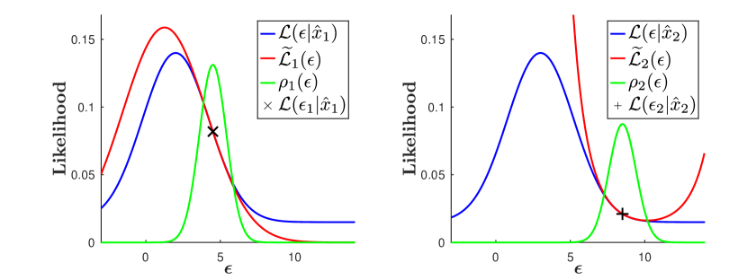
where and . Since we have assumed that is more compactly supported than , it follows that is also more compactly supported than and therefore is more compactly supported than as well. Consequently, the reparameterized likelihood factors , which are the denominators in , can be efficiently approximated locally with exponentiated quadratics as illustrated in figure 1. The quadratics are determined by a second order Taylor series expansion of the logarithm of the factors calculated at the point and the approximation is specified by the following expressions:
| (14) | |||
| (15) | |||
| (16) |
where we have used for short of .
It is interesting to note that the approximations of the reparameterized likelihood factors look remarkably similar to the approximate terms in Minka (2001b). This is not a coincidence since both have the same functional form of exponentiated quadratic and both approximate likelihood factors. However, is a global approximation and is defined as a scaled ratio between the new variational distribution and the old Minka (2001b). In contrast, is a local approximation and is determined by the second order Taylor series expansion of at . Furthermore, the two are used in very different contexts and for different purpose.
3.3 Analytically Solving the Integrals
Since both and are exponentiated quadratics, the product is also an exponentiated quadratic and after some rearranging can be expressed as follows:
| (17) |
where
| (18) | |||
| (19) | |||
| (20) |
It can be verified that is a proper Gaussian because is strictly positive.
Alternatively, the Laplace approximation can also be used to locally approximate by finding its mode and computing the variance at the mode. However, finding the mode of requires in itself iterative approximation, which would add significant complexity to the whole method because it has to be performed for each data point.
3.4 Extension to Multidimensional Data
Let be the dimensionality of the data. Since the data space can be scaled and rotated arbitrarily, we can assume without loss of generality that the multivariate Gaussian in the observation density is spherical. Consequently, the gradient over the mean of the variational distribution is separable and can be broken into one dimensional gradients along the principal axes of the ellipsoid defining the variational distribution. Similarly, the gradient over the diagonal elements of is also separable and can be broken into one dimensional variance gradients along the principal axes. However, efficiently determining the off-diagonal elements of is not trivial and a possible approach can be to adjust the principal axes by employing principal component analysis in an iterative optimization scheme, essentially breaking the multidimensional problem into multiple single dimensional ones.
3.5 Applicability to Non-Gaussian Distributions
The main restriction for the applicability of the proposed approximation to non-Gaussian distributions comes from the reparameterization trick, which does not easily generalize to other common distributions, such as the gamma or beta. While a number of methods have been proposed to circumvent that problem (Ruiz et al. (2016), Figurnov et al. (2018)), these have been developed with stochastic approximation of the expectation in mind and are not readily applicable to analytical integration. A possible solution for this limitation can be to approximate the target distribution with a Gaussian mixture and extend the proposed ELBO gradient approximation to handle Gaussian mixtures.
4 Maximizing ELBO
To test the proposed analytical approximation of the ELBO gradient we integrate it in the expectation step of an EM algorithm for ELBO maximization, as specified in algorithm 1. The approximation allows the expectation step to be applied directly on the ELBO gradient rather than on ELBO itself. In the maximization step we then derive update rules for optimization of the variational distribution parameters and through fixed-point iteration. Our aim is to construct linear update rules by keeping constant, with respect to the current values of and , all terms that are limited in range. For each update rule convergence is briefly examined by demonstrating that the update is in the direction of the local maximum stationary point but we leave a detailed convergence analysis for future work.
Since the approximation relies on the assumption that the variational distribution is more compactly supported than the Gaussian distribution in the likelihood factors, to satisfy that condition during the first few iterations when is large we introduce a substitute for , denoted , and initialize it to . The factor is chosen because it provides acceptable worst case error of the approximation. The substitute is then gradually reduced with each iteration of the algorithm according to the rule until it reaches the value of . The value of is used in place of in all expressions of the gradient approximation and the update rules but for clarity purposes we do not specify it explicitly. In addition, to prevent from breaking the assumption of compact support it is constrained by the rule at the end of each iteration.
-
1.
Input: data , size , , , , ,
-
2.
Initialize , ,
-
3.
For to convergence or maximum number of iterations
-
(a)
Expectation step: approximate the ELBO gradient and compute , , , , and
-
(b)
Maximization step: update the parameters of the variational distribution and according to the update rules
-
(c)
update , constrain
-
(a)
4.1 Update Rule for the Mean
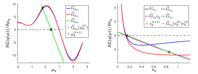
We start by examining the terms that make up as defined in equation (23). These are , , and . If we assume that the probability for a non-clutter data point is greater than zero, it can be readily deduced from its definition in equation (11) that the term is limited to the range . It follows then that falls within the range and therefore so does . Since and , it follows that and therefore because it is an exponent with a negative argument. Since and , it also follows that . Consequently, since is a product of the above terms, it follows that is limited to the range . Therefore, to derive the update rule for the mean we keep constant with respect to the current value of . Setting the approximate gradient equal to zero in equation (21) we then solve the resulting equation for :
| (26) |
where is the updated value and is the current value. The corresponding update function is presented in figure 2 and is defined by the linear expression:
| (27) |
To confirm that is updated in the direction of the local maximum we demonstrate that the slope of the update function is negative. Let be the local maximum stationary point ( and ). If it follows that , since is the gradient. At the same time, if and the slope of is negative it follows that , and therefore the update is in the direction of the local maximum. Similarly, if it follows that and , and therefore the update is again in the direction of the local maximum. Since we already established that is positive, it follows from equation (27) that the slope of is negative and therefore is always updated in the direction of the local maximum.
4.2 Update Rule for the Variance
We start by multiplying equation (22) with to eliminate in the denominator. The resulting function is illustrated in figure 2 and can be expressed as follows:
| (28) |
Next, we examine the terms and . Since we already established that , and , it follows from the definition of in equation (24) as a product of these terms that . Since , and , it follows that and consequently . In addition, the term is also limited to the range . Therefore, to derive the update rule for the variance we keep the terms , , and constant with respect to the current value of . Setting the approximate gradient equal to zero, we then solve the resulting linear equation, obtaining the following update rule for the variance:
| (29) |
where is the updated value and is the current value. The corresponding update function is presented in figure 2 and is formulated by the linear expression:
| (30) |
To confirm that is updated in the direction of the local maximum we verify that the slope of is negative. Since we already established that is positive, it follows from equation (30) that the slope of is negative and therefore is always updated in the direction of the local maximum.
In addition, we demonstrate that equation (29) produces valid updates () by examining the update function at . In that case the term is equal to zero because is finite. Since and , it follows that the term . Consequently, the update function is strictly positive at and since, as already established, its slope is negative, it follows that the root is strictly positive and therefore is a valid update for .
5 Comparative Testing
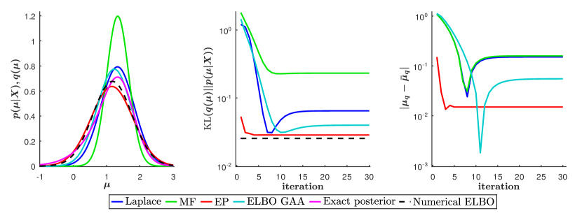
We test the proposed method for analytical approximation of the ELBO gradient against classical deterministic approaches such as the Laplace approximation, expectation propagation and mean-field variational inference. Our implementation of the Laplace approximation and mean-field variational inference is based on the description of the algorithms in Bishop (2006) and for expectation propagation we use Minka (2001a). The test data is generated from the clutter problem observation density as defined in equation (4), for one dimensional data and using the same parameters as specified in Minka (2001b): , , Gaussian distribution in the observation density , number of data points and we also assume the same prior distribution . The aim is to determine how well the proposed method approximates the posterior distribution in comparison to the other three methods. As a measure of goodness of approximation we use the KL divergence between the variational distribution and the posterior, . This is calculated by numerically evaluating the log marginal likelihood and the evidence lower bound for each method. In addition, a baseline of best achievable approximation is provided for reference by numerically maximizing ELBO. We denote the mean of the baseline variational distribution and use it to define absolute error rates for the means of the tested variational distributions.
The result of one test with 20 data points is presented in figure 3. A data sample with a rather skewed posterior is selected to give the tested methods a challenge. To summarize the test results, the proposed method scores second behind EP in terms of KL divergence and absolute error of the mean, beating both mean-field variational inference and the Laplace approximation by a significant margin. It also demonstrates a good rate of convergence, slightly worse than MF and Laplace. Furthermore, in contrast to EP, which can fail to converge (Minka (2001a)) or in certain circumstances can produce negative (Minka (2001b)), the proposed method appears to not suffer from problems with convergence and as demonstrated in section 4.2 is guaranteed to have strictly positive .
An interesting observation is that just before convergence is reached the KL divergence of the proposed method increases slightly. This is easily explained. The optimization of the variational distribution parameters is performed with respect to the local maximum stationary point defined by the approximate ELBO gradient, which is slightly different from the stationary point of the real ELBO gradient due to the imperfection of the approximation. As a result, when the parameters are far away from the two stationary points, updating them towards the appproximate stationary point means also a decrease in the distance to the real stationary point and hence a reduction of the KL divergence. However, when the parameters are very close to the real stationary point updating them towards the appproximate stationary point may in some cases increase the distance to the real stationary point and hence increase the KL divergence.
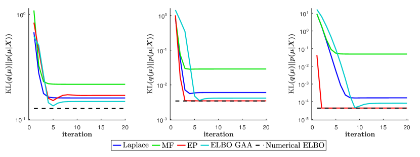
Figure 4 illustrates the performance of the tested algorithms for 5, 10 and 100 data points. As can be observed, the proposed method performs well for all three cases and for the case of 5 data points even comes out the best in terms of KL divergence.
In terms of computational complexity, the proposed method is linearly dependent on the number of data points just like the other three methods. However, the number of exponentiation operations is versus for EP, MF and Laplace. Furthermore, there are also square roots and the number of arithmetic operations is generally larger.
6 Conclusion
We describe a method for analytical approximation of the ELBO gradient in the context of the clutter problem. The approximation is integrated into the expectation step of an EM algorithm for ELBO maximization and update rules for optimizing the variational parameters are derived. We test the proposed method against classical deterministic approaches such as the Laplace approximation, expectation propagation and mean-field variational inference, and the method demonstrates good accuracy and rate of convergence for both small and large number of data points. The computational complexity is linearly dependent on the number of data points, but the number of mathematical operations is somewhat larger compared to the other three algorithms in the test. We provide limited convergence analysis for the update rules of the developed EM algorithm and, while empirical data suggests convergence is reliable, a detailed analytical proof of convergence is a primary research task for the future. Another area where the proposed method requires further work is the extension to multidimensional data observations and the handling of non-Gaussian distributions. While the proposed method provides a solution for the maximization of ELBO by optimizing the variational distribution parameters it does not offer a means to calculate the actual value of ELBO and as a result can not be used for model selection.
References
- Bishop (2006) C. M. Bishop. Pattern Recognition and Machine Learning. Springer New York, 2006.
- Blei et al. (2017) D. M. Blei, A. Kucukelbir, and J. D. McAuliffe. Variational inference: A review for statisticians. Journal of the American Statistical Association, 112:859–877, 2017.
- Dempster et al. (1977) A. P. Dempster, N. M. Laird, and D. B. Rubin. Maximum likelihood from incomplete data via the em algorithm. Journal of the Royal Statistical Society. Series B, 39:1–38, 1977.
- Figurnov et al. (2018) M. Figurnov, S. Mohamed, and A. Mnih. Implicit reparameterization gradients. In Advances in Neural Information Processing Systems (NIPS 2018), 2018.
- Jankowiak and Obermeyer (2018) M. Jankowiak and F. Obermeyer. Pathwise derivatives beyond the reparameterization trick. In Proceedings of the 35th International Conference on Machine Learning, volume 80, pages 2235–2244, 2018.
- Jordan et al. (1999) M. I. Jordan, Z. Ghahramani, T. S. Jaakkola, and L. K. Saul. An introduction to variational methods for graphical models. Machine Learning, 37:183–233, 1999.
- Kingma and Welling (2014) D. P. Kingma and M. Welling. Auto-encoding variational bayes. In International Conference on Learning Representations, ICLR 2014, 2014.
- Minka (2001a) T. P. Minka. Expectation propagation for approximate bayesian inference. In Proceedings of the Seventeenth Annual Conference on Uncertainty in Artificial Intelligence (UAI-2001), pages 362–369, 2001a.
- Minka (2001b) T. P. Minka. A Family of Algorithms for Approximate Bayesian Inference. PhD thesis, Department of Electrical Engineering and Computer Science, Massachusetts Institute of Technology, 2001b.
- Paisley et al. (2012) J. Paisley, D. Blei, and M. Jordan. Variational bayesian inference with stochastic search. In Proceedings of the 29th International Conference on Machine Learning, ICML 2012, volume 2, 2012.
- Ranganath et al. (2014) R. Ranganath, S. Gerrish, and D. Blei. Black box variational inference. In Proceedings of the Seventeenth International Conference on Artificial Intelligence and Statistics, volume 33, pages 814–822, 2014.
- Ruiz et al. (2016) F. R. Ruiz, M. K. Titsias, and D. M. Blei. The generalized reparameterization gradient. In Advances in Neural Information Processing Systems (NIPS 2016), 2016.
- Zhang et al. (2019) C. Zhang, J. Bütepage, H. Kjellström, and S. Mandt. Advances in variational inference. IEEE Transactions on Pattern Analysis and Machine Intelligence, 41(8):2008–2026, 2019.
Appendix A Approximating the Terms with a Gaussian
Substituting with its definition from equation (11) we have:
| (31) |
Since both and are Gaussian, their product is conveniently also Gaussian, wich we denote :
| (32) |
where and . Rearranging and simplifying equation (32) we obtain:
| (33) |
The denominator of is the reparameterized likelihood factor and, because of the assumption for compact support of the variational distribution, it can be efficiently approximated locally at the point with an exponentiated quadratic, where the quadratic is derived by a second order Taylor series expansion of at :
| (34) | |||
| (35) | |||
| (36) |
Deriving is straightforward and for we use the product rule of derivatives:
| (37) |
We then apply the product rule of derivatives also to and rearrange:
| (38) |
Replacing back in equation (37) we obtain:
| (39) | |||
| (40) |
Next we substitute in the numerator of with its definition and simplify the resulting expression:
| (41) | |||
| (42) | |||
| (43) |
We then rewrite equation (34) by completing the square inside the exponent, where for simplicity we have defined and :
| (44) |
The product can be formulated then as follows:
| (45) |
Substituting in with we cancell out the terms and substituting with the expression for the product becomes:
| (46) |
Since is the numerator of as defined in equation (43) and is the denominator, the product is simplified to the following:
| (47) |
We then carry out the multiplication of the two exponentiated quadratics:
| (48) | |||
| (49) | |||
| (50) | |||
| (51) |
Expanding and rearranging equations (49), (50) and (51) we obtain:
| (52) | |||
| (53) | |||
| (54) | |||
| (55) | |||
| (56) | |||
| (57) |
| (58) | |||
| (59) | |||
| (60) | |||
| (61) | |||
| (62) |
| (63) | |||
| (64) | |||
| (65) | |||
| (66) | |||
| (67) | |||
| (68) | |||
| (69) |
Since , it follows that and therefore equation (48) represents a proper Gaussian which results in the final expression for as a Gaussian approximation of :
| (70) | |||
| (71) | |||
| (72) | |||
| (73) |
Appendix B Solving the Integrals
To compute the integral in equation (10) we substitute with its approximation from equation (17):
| (74) |
Modifying the term to and recognizing that while is a constant with regards to , we carry out the integration:
| (75) |
Next, we substitute with its definition from equation (19) and rearrange:
| (76) |
Further rearranging, we obtain the final expression for :
| (77) | |||
| (78) |
To compute the integral in equation (12) we substitute with its approximation from equation (17):
| (79) |
Modifying the term to we recognize that , , and is a constant with respect to . Carrying out the integration in equation (79) then results in the following expression:
| (80) |
Next, we substitute in with its definition from equation (19) and rearrange:
| (81) | |||
| (82) |
Substituting equation (82) back in equation (80) we obtain the final expression for :
| (83) | |||
| (84) | |||
| (85) |