Capturing the Macroscopic Behaviour of Molecular Dynamics with Membership Functions

Abstract

Markov processes serve as foundational models in many scientific disciplines, such as molecular dynamics, and their simulation forms a common basis for analysis. While simulations produce useful trajectories, obtaining macroscopic information directly from microstate data presents significant challenges. This paper addresses this gap by introducing the concept of membership functions being the macrostates themselves. We derive equations for the holding times of these macrostates and demonstrate their consistency with the classical definition. Furthermore, we discuss the application of the ISOKANN method for learning these quantities from simulation data. In addition, we present a novel method for extracting transition paths based on the ISOKANN results and demonstrate its efficacy by applying it to simulations of the $\mu$-opioid receptor. With this approach we provide a new perspective on analyzing the macroscopic behaviour of Markov systems.

1 Introduction

Many physical processes are best understood as autonomous Markov processes (e.g. [8]). A common mathematical model for them are stochastic differential equations which allow to predict the probability for the future evolution of the system. Markovianity means, that this probability is just depending on the initial condition of the system. Solving the initial value problem is referred to as simulation of the system. The states of the generated trajectory are denoted as the micro states of the system.

As an illustration, consider the field of biomolecular system simulation [7]. Here a common mechanism being studied is the transformation of an inactive micro state of a receptor protein into an active state (by accordingly changing the coordinates of its atoms). The process can be mathematically modeled by the overdamped Langevin dynamics, a stochastic differential equation for the 3D coordinates of each atom in the protein and the solvent [6]. Typically these are analysed by simulation of the model, resulting in trajectories in a high-dimensional space.

However, often, the main focus of interest lies on the macro state behaviour of the system. A possible question to answer would be: What is the mean first passage time for an inactive receptor protein to become active? The two macro states in this regard are denoted as “inactive” versus “active”. At first glance, macro states $S$ are subsets of the set of micro states $\Omega$. In general, when given a starting set $S\subset\Omega$ of the system we want to know, how long on average the process stays in this set [19]. How long does a trajectory starting in the inactive macro state remains there before leaving it, i.e. switching to the active macro state? The answer is given by the mean holding time $t_{\text{mh}}(\boldsymbol{x})$ defined by the integral:

$$t_{\text{mh}}(\boldsymbol{x})=\int\limits_{0}^{\infty}p_{S}(\boldsymbol{x},t)\,dt,$$

where $\boldsymbol{x}$ denotes the micro state of the system (the starting point ${x}(0)=\boldsymbol{x}$ of the trajectory) and the function $p_{S}(\boldsymbol{x},t)$ denotes the probability that a trajectory is still in set $S$ and has never left it during the whole time interval $[0,t]$. If $t_{\text{mh}}(\boldsymbol{x})$ denotes the “expected time until the system reacts”, then

$$\boldsymbol{r}(\boldsymbol{x})=-\nabla t_{\text{mh}}(\boldsymbol{x})=-\nabla\int\limits_{0}^{\infty}p_{S}(\boldsymbol{x},t)\,dt$$

points into the direction where this time decreases the most. This can be seen as the micro-state-dependent reaction path direction $\boldsymbol{r}(\boldsymbol{x})$.

There is a conceptual problem now. We want to know the mean holding time for the macro state and not for every single micro state, but $t_{\text{mh}}$ is a function of the micro states – the mean holding time in $S$ depends on the starting point. Speaking of the “mean holding time of the macro state $S$” would only make sense if it was independent of the micro-states position inside that macro state, i.e. allowing for a separation of the type

$$p_{S}(\boldsymbol{x},t)=1\!\!1_{S}(\boldsymbol{x})\,\mathrm{e}^{-c_{1}t},$$ (1)

where $1\!\!1_{S}$ is the indicator function of the set $S$. The constant $c_{1}>0$ then corresponds to the exit rate of $S$, because in this case $t_{\text{mh}}(\boldsymbol{x})=1\!\!1_{S}(\boldsymbol{x})\,\frac{1}{c_{1}}$ is independent from the choice of the starting point in $S$. This decomposition, however, is not possible in general and corresponds to instantaneous transitions which do not provide reaction paths inside $S$.

Classically the computation of (micro-state) mean holding times in the case of an $S$-based theory is provided by solving a partial differential equation [9]:

$${\cal L}^{\ast}t_{\text{mh}}(\boldsymbol{x})=-1,$$

for all $\boldsymbol{x}\in S$ with the boundary condition $t_{\text{mh}}(\boldsymbol{x})=0$ for all $\boldsymbol{x}\not\in S$. In this equation the differential operator ${\cal L}^{\ast}$ is the infinitesimal generator of the Koopmann operator of an autonomous Markov process. If the decomposition $t_{\text{mh}}(\boldsymbol{x})=1\!\!1_{S}(\boldsymbol{x})\,\frac{1}{c_{1}}$ would be valid, then this equation would read

$${\cal L}^{\ast}1\!\!1_{S}(\boldsymbol{x})=-c_{1}1\!\!1_{S}(\boldsymbol{x}).$$ (2)

This has a trivial solution $S=\Omega$ and $c_{1}=0$ (the process never leaves $\Omega$). The constant function $1\!\!1_{\Omega}$ is an eigenfunction of ${\cal L}^{\ast}$. However, this is not a desired solution.

How can we solve this conceptual problem?

When deriving exit rates for biomolecular processes, then the macro states of this system can not be rigorously described as subsets $S$ in micro state space. Rather, transitions are gradual from something that is more inactive to something that can be described as more active. We propose replacing $1\!\!1_{S}$ by a membership function $\chi:\Omega\rightarrow[0,1]$ which quantifies how much a micro state ${\boldsymbol{x}}\in\Omega$ belongs to the starting macro state. The theoretical background of our article, therefore, starts with the desired separation of space and time via

$$p_{\chi}(\boldsymbol{x},t)=\chi(\boldsymbol{x})\,\mathrm{e}^{-c_{1}t}.$$ (3)

By definition it satisfies the exponential decay of $p_{\chi}$ in $t$ and at $t=0$ the probability to be assigned to the starting state is given by $\chi$. This gives rise to the fundamental idea of identifying the macrostate with the membership function: $\chi$ is the macro state and the macro state is given in and through $\chi$. At this point we have not provided a method to compute $\chi$ yet. $\chi$ can not be chosen arbitrarily. In order to preserve the Markovian long term behavior of the system a projection of the micro system to two different macro states has to be based on an invariant subspace of ${\cal L}^{\ast}$ [18, 20] which leads to [19]:

$${\cal L}^{\ast}\chi(\boldsymbol{x})=-c_{1}\chi(\boldsymbol{x})+c_{2}(1-\chi(\boldsymbol{x})).$$ (4)

Here $\chi$ and $1-\chi$ describe two complementary macrostates of the system. They can be computed using PCCA+ [2] or ISOKANN [11, 15] and form an invariant subspace of ${\cal L}^{\ast}$ which also guarantees long-term consistency with the original dynamics [20].

In Section 2 of this paper we demonstrate that our macro state formalism based on the $\chi$-function is consistent with the traditional set-based method: We show that when the $\chi$-functions approach indicator functions the $\chi$ based equations reduce to the classical ones. We further motivate its physical meaning by giving a path-based interpretation of the resulting holding probabilities in terms of the Feynman-Kac formula.

In Section 3, we will suggest an approach to apply these theoretic results to extract transition paths from a set of given samples, before demonstrating its application to a molecular system given by the $\mu$-opioid receptor in Section 4.

2 Theory of macroscopic exit rates

In the following, a consistent theory about macroscopic quantities based on a membership function $\chi:\Omega\rightarrow[0,1]$ is derived. More precisely, the following quantities of interest are discussed:

• the definition of a macro state via $\chi(\boldsymbol{x})$,

• the corresponding position-independent exit rate $c_{1}$,

• the mean holding time $t_{\text{mh}}(\boldsymbol{x})$, and

• the reaction direction $\boldsymbol{r}$ proportional to the gradient $-\nabla\chi$.

Note that computing reaction directions $\boldsymbol{r}$ is possible for sets $S$, too, as described in the introduction. However, for sets we do not get this simple gradient form $-\nabla\chi$. The theory in this section is largely based on [19, 3]. We will extend the theory with statements about consistency and use it to support of the interpretation of $\chi$ as macro states, as explained in the introduction. The computation of $\chi$ will play an important role in our bio-molecular example, see section 4.

2.1 Defining macro states via membership functions

The starting point in the introduction is that $p_{\chi}=\chi\mathrm{e}^{-c_{1}t}$ would be a way to define holding times of macro states from a conceptual point of view to be able to interpret $c_{1}$ as an exit rate. The choice of $\chi$ is not arbitrary, but motivated by the necessity of an invariant subspace projection leading to (4). At this point it is not yet shown that $p_{\chi}$ when using the solution $\chi$ of (4) is consistent with the stochastic meaning of a holding probability. We will now demonstrate that it converges to the established definition if $\chi$ becomes the indicator function of a set.

We start by recalling some basic definitions. Let the state space $\Omega$ of a molecular system comprising $N$ atoms be given as $\Omega=\mathbb{R}^{3N}$ where the position of each individual atom is described by three Cartesian coordinates. Let $\rho(\boldsymbol{x},t):\Omega\times\mathbb{R}\to[0,1]$ denote the probability density distribution of states of the non-linear stochastic dynamics at time $t$. More precisely, the dynamics is given as a Markov process for which an infinitesimal generator $\mathcal{L}:L^{1}(\Omega)\rightarrow L^{1}(\Omega)$ (a differential operator, e.g. the Fokker-Planck operator) can be constructed that captures this time-dependent stochastic process. This operator is linear and describes the infinitesimal propagation of $\rho(\boldsymbol{x},t)$:

$$(\mathcal{L}\rho)(\boldsymbol{x},t)=\frac{\mathrm{d}}{\mathrm{d}t}\rho(\boldsymbol{x},t).$$ (5)

It also gives rise to its adjoint generator $\mathcal{L}^{\ast}:L^{\infty}(\Omega)\rightarrow L^{\infty}(\Omega)$ which propagates observables instead of state densities. The partial differential equation (4) defining $\chi$ is formulated in terms of this adjoint. In this regard $\chi$ can also be interpreted as an observable, i.e. the measurement of the macro state. To allow for their interpretation as holding probability we are interested in solutions $\chi(\boldsymbol{x}):\Omega\to[0,1]$ with corresponding constants $c_{1}>0,c_{2}>0$.

At this point the holding probabilities can be defined by multiplying the solution $\chi$ of (4) with $\mathrm{e}^{-c_{1}t}$,

$$p_{\chi}(\boldsymbol{x},t):=\chi(\boldsymbol{x})\mathrm{e}^{-c_{1}t}$$ (6)

such that (4) becomes:

$$\mathcal{L}^{\ast}p_{\chi}=-c_{1}p_{\chi}+c_{2}p_{\chi}\frac{1-\chi}{\chi}.$$ (7)

Rearranging results in:

$$\mathcal{L}^{\ast}p_{\chi}-c_{2}p_{\chi}\frac{1-\chi}{\chi}=-c_{1}p_{\chi}.$$ (8)

Due to the relationship

$$\frac{\partial}{\partial t}p_{\chi}=\frac{\partial}{\partial t}\chi(\boldsymbol{x})\mathrm{e}^{-c_{1}t}=-c_{1}\chi(\boldsymbol{x})\mathrm{e}^{-c_{1}t}=-c_{1}p_{\chi}$$ (9)

Eq. (8) can also be represented as follows:

$$\mathcal{L}^{\ast}p_{\chi}-c_{2}p_{\chi}\frac{1-\chi}{\chi}=\frac{\partial}{\partial t}p_{\chi}.$$ (10)

The solution of the partial differential equation (10) together with the initial condition

$$p_{\chi}(\boldsymbol{x},0)=\chi(\boldsymbol{x})\mathrm{e}^{-c_{1}\cdot 0}=\chi(\boldsymbol{x})$$ (11)

can be given in terms of the Feynman-Kac formula [19, 3, 5]:

$$p_{\chi}(\boldsymbol{x},\tau)=\mathbb{E}\left[\chi(\boldsymbol{x}_{\tau})\cdot\text{exp}\left(-c_{2}\int^{\tau}_{0}\frac{1-\chi(\boldsymbol{x}_{t})}{\chi(\boldsymbol{x}_{t})}\mathrm{d}t\right)\Big{|}\boldsymbol{x}_{0}=\boldsymbol{x}\right].$$ (12)

It allows us to interpret the solution as an expectation over realizations of the stochastic process and therefore builds the bridge from an abstract definition to its interpretation as a probability.

To this end let us consider the case where $\chi\approx 1\!\!1_{S}$. Then $p_{\chi}$ is the expectation over trajectories starting in $\boldsymbol{x}_{0}$. Once any such trajectory leaves the set $S$ the integral becomes infinite and exponential function evaluates to $0$. Otherwise the exponential stays $1$, as well as $\chi(\boldsymbol{x}_{\tau})=1$. We therefore recover the definition of classical holding probability $p_{\chi}(\boldsymbol{x},\tau)=p_{S}(\boldsymbol{x},\tau)$ in (1), see also (9) and (10) in [19], as well as (3.31) in [14].

With regard to this interpretation, $p_{\chi}(\boldsymbol{x},t)$ is seen as the holding probability of the macro state $\chi$. Due to the separated term $\mathrm{e}^{-c_{1}t}$ in (6), the holding probability decreases exponentially with the decay constant $c_{1}$. This means that $c_{1}$ is the exit rate from $\chi$. Since the function value of $p_{\chi}(\boldsymbol{x},0)=\chi(\boldsymbol{x})$ is interpreted as a holding probability, it is necessary that $\chi$ can only take values in the interval $[0,1]$.

The time integral over the holding probability is the mean holding time $t_{\text{mh}}(\boldsymbol{x})$, which is proportional to the inverse of the exit rate $c_{1}$:

$$t_{\text{mh}}(\boldsymbol{x})=\int^{\infty}_{0}p_{\chi}(\boldsymbol{x},t)\mathrm{d}t=\int^{\infty}_{0}\chi(\boldsymbol{x})\mathrm{e}^{-c_{1}t}\mathrm{d}t=\lim_{t\to\infty}\left[-\frac{1}{c_{1}}\chi(\boldsymbol{x})\mathrm{e}^{-c_{1}t}\right]^{t}_{0}=\frac{1}{c_{1}}\chi(\boldsymbol{x}).$$ (13)

The mean holding time immediately leads to a definition of a reaction direction: Following the gradient of $t_{\text{mh}}$ increases the time until “a reaction takes place”. Therefore by defining the reaction direction $\boldsymbol{r}:\Omega\rightarrow\mathbb{R}^{3N}$,

$$\boldsymbol{r}(\boldsymbol{x})=-\nabla t_{\text{mh}}(\boldsymbol{x})=-\frac{1}{c_{1}}\nabla\chi(\boldsymbol{x})\propto-\nabla\chi(\boldsymbol{x}),$$ (14)

we obtain a vector field along which the mean holding time decreases uniformly and which is proportional to $\nabla\chi$. This also means that $\chi$ itself can be understood as an order parameter, i.e. a reaction coordinate for the system. Note that we obtain this time independent result only as a consequence of the initial time separation ansatz for $p_{\chi}$. By integrating curves tangential to $\boldsymbol{r}$ one can obtain reaction paths in $\Omega$. In Section 3 we will make use of the order parameter interpretation to subsample a representative reactive path from a given pool of simulation data.

The possibility of calculating these quantities of interest from (4) is a motivation to develop an efficient method for solving this equation. We will now show how to express these quantities in terms of the Koopman operator, before discussing ISOKANN, an algorithm for their computation.

2.2 Membership functions from Koopman operator

So far the description of $\chi$ was based on the infinitesimal generator $\mathcal{L}^{\ast}$ but a suitable analytical solution of the corresponding partial differential equation (4) is not available. However, it is possible to transform (4) into an equation for which a constructive solution is possible. We will now show how we can similarly formulate it in terms of the Koopman operator $\mathcal{K}$ and how we can switch between the formalisms. The problem of its actual solution will then be addressed in the next subsection.

The Koopman operator $\mathcal{K}^{\tau}$ is the time-integral or solution operator of $\mathcal{L}^{\ast}$ for some lag-time $\tau>0$ and can be formally defined as $\mathcal{K}^{\tau}=\mathrm{e}^{\tau\mathcal{L}^{\ast}}$. It can also be defined by its action on observable functions $f:\Omega\rightarrow\mathbb{R}$:

$$(\mathcal{K}^{\tau}f)(\boldsymbol{x}):=\mathbb{E}\big{[}f(x(\tau))\mid x(0)=\boldsymbol{x}\big{]},$$ (15)

where the expectation is taken over independent realizations $x$ of the process, starting in $x(0)=\boldsymbol{x}$. It can therefore be interpreted as the operator returning the expected measurements $\mathcal{K}^{\tau}f$ of an observable $f$ after a lag time $\tau$. In this way, its action can be approximated using Monte-Carlo estimates over simulations, making it particularly suitable for applications.

To transform (4) into an equation for $\mathcal{K}^{\tau}$ we substitute

$$\alpha=c_{1}+c_{2}$$ (16)

to arrive at the following equation:

$$\mathcal{L}^{\ast}\chi=-\alpha\chi+c_{2}.$$ (17)

This shows that ${\cal L}^{\ast}$ acts as a shift-scale operator if and only if $\chi$ solves (4). Making use of the formal exponential representation of $\mathcal{K}^{\tau}$ and its series expansion one obtains [19, 3]:

$$\mathcal{K}^{\tau}\chi=\mathrm{e}^{-\tau\alpha}\chi+\frac{c_{2}}{\alpha}(1-\mathrm{e}^{-\tau\alpha}).$$ (18)

Setting

$$\gamma_{1}=\mathrm{e}^{-\tau\alpha},\quad\gamma_{2}=\frac{c_{2}}{\alpha}(1-\gamma_{1})$$ (19)

this becomes:

$$\mathcal{K}^{\tau}\chi=\gamma_{1}\chi+\gamma_{2}.$$ (20)

So, just as with equation (17), $\mathcal{K}^{\tau}$ acts as a shift-scale if and only if $\chi$ is a solution to (4). Note however, that its shift ($\gamma_{1}$) and scale ($\gamma_{2}$) parameters differ.

The above identities allow us to switch between the infinitesimal generator and Koopman framework. In particular, we can compute the exit rate $c_{1}$ from the Koopman parameters $\gamma_{1}$ and $\gamma_{2}$:

$$\alpha=-\frac{\text{ln}\gamma_{1}}{\tau},\quad c_{2}=\frac{\alpha\gamma_{2}}{1-\gamma_{1}},\quad c_{1}=\alpha-c_{2}.$$ (21)

By evaluating $\chi$ and $\mathcal{K}^{\tau}\chi$ at sample points $\boldsymbol{x}\in\Omega$ we can therefore estimate the exit rate $c_{1}$ by solving the linear regression problem (20).

2.3 ISOKANN for computing membership functions

The ISOKANN (Invariant subspaces of Koopman operators learned by a neural network) method [11, 16, 15] is a fixed-point iteration which combines the use of a neural network for representing the high-dimensional $\chi$ function with the Koopman formalism to enable its training on simulation data.

On convergence it returns $\chi$ that solves (4), (17) and (20). Solving the partial differential equations involving $\mathcal{L}^{\ast}$ directly is not feasible due to the high dimensionality of molecular systems. Molecular simulations on the other hand enable us to estimate the action of $\mathcal{K}^{\tau}$ on an observable. For this reason, ISOKANN attempts to solve (20) by using the action of $\mathcal{K}^{\tau}$ for the calculation of $(\mathcal{K}^{\tau}\chi_{i})(\boldsymbol{x})$, where $\chi_{i}$ is the $i$-th iterate of $\chi$ and $\boldsymbol{x}$ is a training point. It approximates the expectation value

$$(\mathcal{K}^{\tau}\chi_{i})(\boldsymbol{x}):=\mathbb{E}\big{[}\chi_{i}(x(\tau))\mid x(0)=\boldsymbol{x}\big{]},$$ (22)

by a Monte-Carlo estimate over trajectory simulations $x$ starting in different starting points $\boldsymbol{x}$. The next iterate is then given by the shift-scaled $\mathcal{K}^{\tau}\chi_{i}$:

$$\chi_{i+1}:=\frac{\phantom{\|}\mathcal{K}^{\tau}\chi_{i}-\min(\mathcal{K}^{\tau}\chi_{i})\phantom{\|_{\infty}}}{{\|\mathcal{K}^{\tau}\chi_{i}-\min(\mathcal{K}^{\tau}\chi_{i})\|}_{\infty}},$$ (23)

which is motivated by inverting the shift and scale of (20), such that the solution $\chi$ to (20) is indeed a fixed point. ISOKANN is based on the power method, an iterative method used to obtain the dominant eigenfunction of a linear operator. In ISOKANN additional scaling and shifting in each iteration ensures that it does not converge to the constant function, but against the membership function $\chi(\boldsymbol{x}):\Omega\to[0,1]$ [16] – similar to targeting the second eigenvalue in the inverse power method. In order to represent the iterates $\chi_{i}$, we approximate them by a neural network. The equality assignment in the iteration (23) thus becomes a supervised learning problem at data points $\boldsymbol{x}$ with labels given by the corresponding right hand side of (23) evaluated on the previous generation of the network. The iterations are then terminated by a stopping criterion which can be either a high correlation coefficient $(\chi_{i}(\boldsymbol{x}_{n}),\chi_{i+1}(\boldsymbol{x}_{n}))_{n}$ or a small empirical loss $\|\chi_{i}-\chi_{i+1}\|_{2}$, indicating that we found an approximate solution to (20).

Assuming infinite data and perfect representation by the neural network, this iteration indeed converges to the slowest solution $\chi$ of (20)[16]. In practice however, for multiple low-lying eigenvalues, this routine can result close to one of multiple possible membership functions (each representing one of these slower processes). In that case the procedure can be repeated and the resulting membership functions can be used to construct an invariant subspace of $\mathcal{K}$.

One of ISOKANN’s main benefits is that it avoids discretizing the state space, which is crucial for the application to high-dimensional systems and avoiding the curse of dimensionality [11]. In the ISOKANN algorithm it is possible to train artificial neural networks by collecting many short-term trajectories of simulation length $\tau$ from different starting points in high-dimensional spaces. Thus, ISOKANN can be applied to many independent short-time trajectories or it can even decide where in $\Omega$ to enrich simulation data [16]. In our illustrative example we will apply it to a small number of medium-length trajectories. The resulting $\chi$ function will then be used to subsample a reactive path from the data, which leads us to the next section.

3 Extracting transition paths from simulations

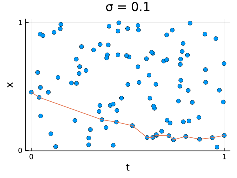
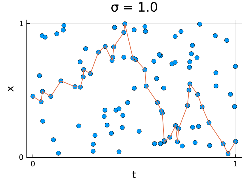
Figure 1: Application of the shortest path algorithm on 100 points distributed uniformly in space and time. For lower $\sigma$ values (left) the path prefers less jumps with small spatial displacement, whilst for higher $\sigma$ (right) the path goes through more points at the cost of more erratic movement.

The learned $\chi$ values can be understood as an order parameter for a set of simulation data in $\Omega$. As shown in (13), the membership values are interpreted to be proportional to mean holding times of a macro state. The level sets of the function $\chi(\boldsymbol{x})$ in this regard correspond to micro states $\boldsymbol{x}$ which “take place simultaneously” in this newly defined time axis. By interpreting this order as a “temporal” parameter we can extract macroscopic transition paths from simulation data. In our illustrative example in section 4, we aim to find temporally ordered paths in $\Omega$. Thus, micro states will be picked forming this path out of given molecular simulation data. In this context, this approach can be seen as a post processing step to classical molecular simulation by which a representation of the slow dynamics contained in the data is obtained.

The problem of extracting a path orthogonal to the level sets of $\chi$ is to find a model to combine temporal with spatial distance.

More precisely, the $\chi$ values will be interpreted as order parameter or artificial time of the transition between macro states. An ordered list $I\subset J=\{1,\dots,N\}$ of samples from simulation points $X_{J}=(\boldsymbol{x}_{j})_{j\in J}$ in $\Omega$ is searched for, such that $\chi(\boldsymbol{x}_{j})$ form an increasing sequence in a smooth way, i.e. without large deviations of $\Delta\boldsymbol{x}_{j}$.

To this end the trajectory samples $\boldsymbol{x}_{j}$ are modelled locally as the result of a Brownian motion $dX_{t}=\sigma dW_{t}$ with their respective $\chi$-value as time. The probability of obtaining a specific set of samples is given by the finite dimensional distribution [9] (in our case we assume $\boldsymbol{b}\equiv 0$ and $\sigma(\boldsymbol{x})\equiv\sigma$ as well as $t=\chi$):

$$p(\boldsymbol{x}_{1},\ldots,\boldsymbol{x}_{n})=\left(\prod^{n-1}_{i=1}(2\pi\sigma^{2}\Delta t_{i})^{-d/2}\right)\exp\left(-\sum^{n-1}_{i=1}\frac{||\boldsymbol{x}_{i+1}-\boldsymbol{x}_{i}||^{2}}{2\sigma^{2}\Delta t_{i}}\right).$$ (24)

Note that this formula is typically used to obtain the probability given a specific set of $\Delta t_{i}$. In our case, it also serves to balance the choice of different time intervals versus spatial jumps. We expect that this can be understood from a Bayesian perspective as prescribing a uniform prior on the number and length of time intervals. For the time being, we consider it a heuristic justified by the results, but further investigation is warranted.

Taking the logarithm allows us to transform this probability into a sum of log probabilities, $\log p(\boldsymbol{x}_{1},\dots,\boldsymbol{x}_{n})=\sum_{i=1}^{n}\log p(\boldsymbol{x}_{i},\boldsymbol{x}_{i+1})$ with

$$\log p(\boldsymbol{x},\boldsymbol{y})=\log\left(\left(2\pi\sigma^{2}\left(\chi(\boldsymbol{y})-\chi(\boldsymbol{x})\right)\right)^{-d/2}\right)-\frac{||\boldsymbol{y}-\boldsymbol{x}||^{2}}{2\sigma^{2}(\chi(\boldsymbol{y})-\chi(\boldsymbol{x}))}.$$ (25)

Finding the maximal likelihood path then corresponds to solving the shortest path problem from a (set of) point(s) $\chi(\boldsymbol{x}_{i})\approx 0$ to a (set of) point(s) $\chi(\boldsymbol{x}_{i})\approx 1$ with edge distance $e_{ij}$ between two points (nodes)

$$e_{ij}=\begin{cases}-\log p(\boldsymbol{x}_{i},\boldsymbol{x}_{j})&\text{if }\chi(\boldsymbol{x}_{i})<\chi(\boldsymbol{x}_{j})\\ \infty&\text{otherwise},\end{cases}$$ (26)

where transitions forward in time (i.e. increasing $\chi$-value) are enforced by the corresponding $\infty$ weight. The corresponding shortest path problem is then solved with the Bellman-Ford algorithm [4].

The parameter $\sigma$ plays the role of a smoothing parameter, balancing the likelihood of jumps in space or time. A high $\sigma$ allows for more erratic jumps over short time-spans while a lower $\sigma$ favors spatially closer jumps possibly necessitating longer time-spans, as illustrated in Figure 1.

Of course the assumption of Brownian motion is far-fetched for an actual molecular system. However, with only finite simulation data, the direction of possible jumps will be dictated mainly by the available data. The Brownian assumption introduces only a small bias which is largely negligible for the choice of paths in the temporal, i.e. $\chi$ direction. In this regard this algorithm can also be understood as a heuristic filtering method to obtain a smooth path through the provided samples along the reaction coordinate from $\chi=0$ to $\chi=1$ (or vice versa).

4 Illustrative Example: Opioid Receptor

To illustrate the added value of $\chi$ computation, we will show an molecular dynamics (MD) example which is part of a pharmaceutical project. We first learned the $\chi$ function from molecular simulation trajectories and applied the described reaction path extraction along $\chi$ to a high-dimensional molecular system consisting of 4734 atoms. The application background is given by understanding pain relief using opioids. Strong painkillers like morphine and fentanyl act upon a special type of receptor in the body known as the $\mu$-opioid receptor (MOR). This receptor is part of the family of opioid receptors and is a G-protein coupled receptor found in various parts of the body such as brain, spinal chord, and gastrointestinal tract [10]. The indiscriminate activation of the MOR across the whole body is one of the causes of severe side-effects of this family of strong pain killers. [1].

However, it is proven that chemical changes at site of inflammation cause the creation of a micro-environment [12]. The knowledge about the local micro-environment can be used to design peripherally restricted strong pain killers with potentially less side-effects [17]. Different micro-environments may lead to different dynamics of the MOR. One possible chemical change of the MOR in inflamed tissue postulates the formation of disulfide bonds as the concentration of reactive oxygens species goes up.

4.1 Algorithmic details

Our input data is taken from $10$ different simulations of MOR. After the primary proximity analysis on the active structure of the MOR (PDB Id:8EF5) a disulfide bond was introduced in the inactive structure of the MOR (PDB Id:7UL4) in between location CYS159 and CYS251 [21, 13]. 10 simulations (with explicit water and with a lipid-bilayer for the MOR) were run. Each simulation spans an interval of 100 nanoseconds, totalling to 1 microsecond.

After simulation, pairwise distances over all $\alpha-$carbons that can be observed to be closer then a threshold ($d_{\max}=$ 12 Å) at least once over the simulation time (normalized to mean 0 and standard deviation 1) serve as input features of the corresponding neural network of the ISOKANN algorithm [15]. The action of the Koopman operator in (23) is estimated with one sample each forward and backward along the time axis, justified by the reversibility of the system. This is used to train the $\chi$-function. With taking forward and backward steps, it is avoided that $\chi$ has all its mass in the terminal point. An uni-directed trajectory would “transport” the $\chi$ values along the trajectory to the final point in the estimation of the Koopman operator.

The neural network is a multilayer perceptron with 3 fully connected hidden layers of size $(6161,336,18)$ with sigmoid activation functions and a single linear output neuron. For the optimisation we use ADAM with a learning-rate of $\eta=1\mathrm{e}{-4}$ with a $L2$ regularization of $\lambda=1\mathrm{e}{-2}$ and a minibatch-size of 128. After training $\chi$ for 30,000 iterations, the described shortest path is extracted with $\sigma=0.7$ resulting in 1,231 selected frames.

Using a large regularization for the neural network enforces a smooth structure to the $\chi$ function which may also be understood as a smoothing of the data and thereby artificially connecting spatially adjacent samples. With regularization ISOKANN, thus, isolates the spatially large transitions which amount to macroscopic changes.

4.2 Application to MOR

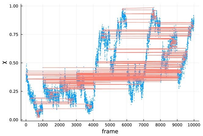
Figure 2: The membership value $\chi(x)$ for each state (frame) $x$ obtained from 10 independent simulations, with each simulation comprising 1,000 frames. The y-axis represents the macroscopic transition, showing that different trajectories cover distinct segments of this transition while exhibiting partial overlap with other trajectories. The extracted reaction path (orange line) progresses from $\chi\approx 0$ to $\chi\approx 1$ while maintaining spatially smooth transitions. Note that it incorporates the data from amongst all 10 simulations and even jumps them where facilitated by small spatial distances in $\Omega$.

ISOKANN serves as an efficient tool to analyse rare events in the simulation of the $\mu$-opioid receptor. As mentioned earlier, finding a solution function $\chi$ of (20) with a low exit rate $c_{1}$ corresponds to the identification of a “reaction coordinate”. In Fig. 2 the resulting $\chi$-values along 10 independent molecular simulations are shown (blue dots). One can see that the lowest and highest values of $\chi$ are not to be found within one trajectory. Using ISOKANN, it is possible to extract the “temporally most distant” frames from the simulation, see Fig. 3. Indeed the $\chi$-values correspond to a reaction coordinate for the transition from an inactive to an active macro state of MOR. Although none of the 10 trajectories simulates this process completely, we can extract the time-determining steps along the reaction path by using the shortest path routine described in section 3. The picked path is rather small in length (1,231 frames, orange in Fig. 2) as compared to entire trajectory of 10,000 stored frames. Using a linear regression to estimate $\gamma_{1},\gamma_{2}$ in (20) we can compute the exit rate for a given lag time $\tau=$ 0.1 ns by (21) resulting in $c_{1}\approx$ 0.06 ns^-1.

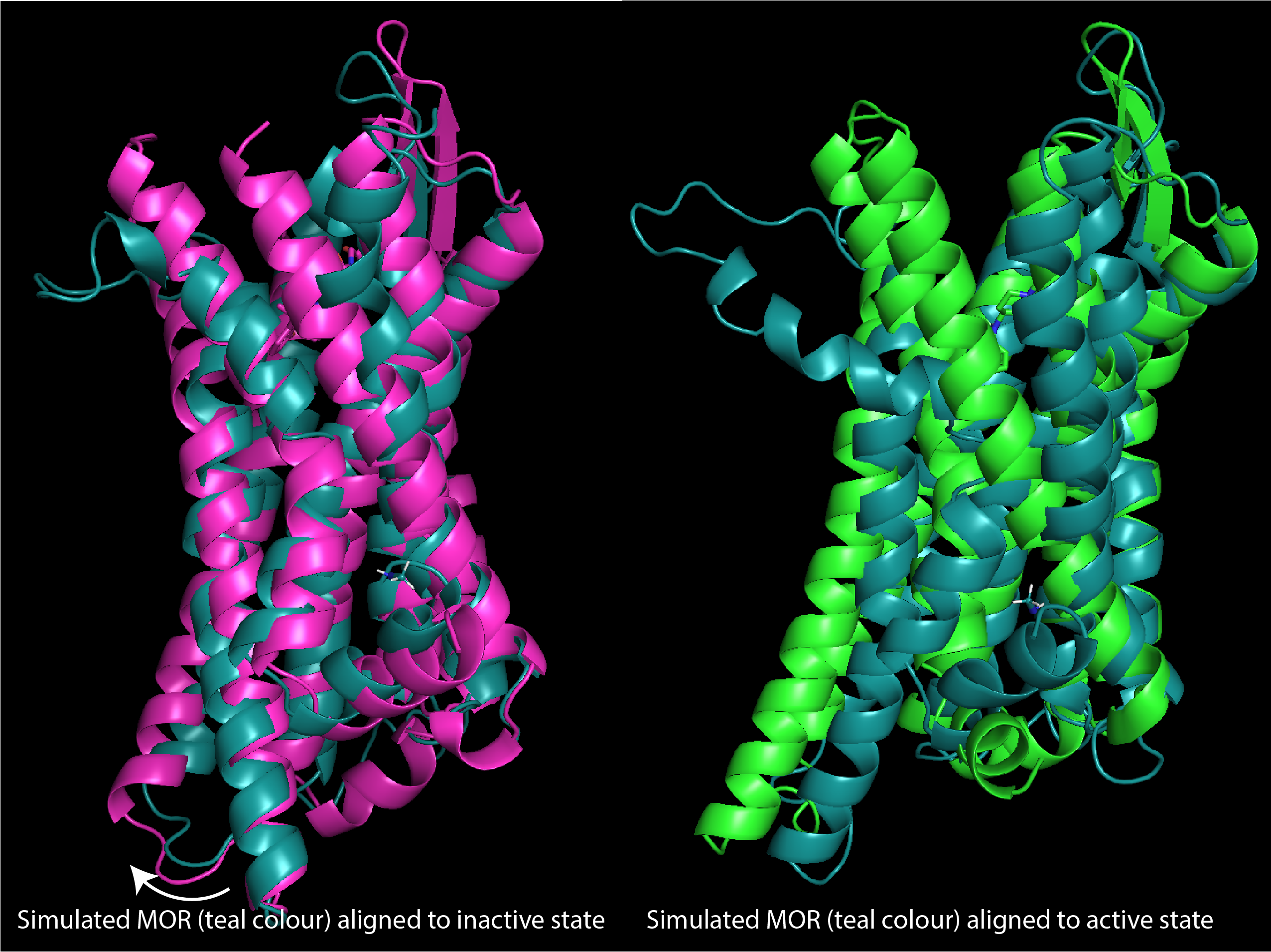
Figure 3: Visualization of the MOR states (teal) at the beginning and end of the transition path in Fig. 2 (orange). The superimposed purple and green structures are known to be representative of the inactive resp. active states (PDB ids 7UL4 and 8EF5). We can see that ISOKANN isolates states similar to these known metastabilities from the simulation trajectories.

In Fig.  3 The modified MOR (teal) with a disulfide bond displays the starting point of the reaction path aligning with the inactive structure of the unmodified, natural state of the MOR (purple). The experiments suggest partial activation of the MOR that is correctly isolated by shortest path analysis represented by movement of the transmembrane helix 6 outwards like it is seen in fully activated, natural MOR crystal strucutre (green). Note that both start and end points of the reactive path where determined without any prior knowledge about the crystal structures.

5 Conclusion

In bridging the conceptual gap between microstate and macrostate analyses, we introduced the notion of mean holding probabilities $p_{\chi}(\boldsymbol{x},t)=\chi(\boldsymbol{x})\mathrm{e}^{-c_{1}t}$ represented in terms of membership functions $\chi$ which we interpret as the macrostate itself. Taking this as a theoretical starting point, the computation of mean holding times $t_{mh}\propto\chi$, which generalize their classical set-based definitions, and of reaction paths along $\boldsymbol{r}\propto-\nabla\chi$ has been shown. Being proportional to a mean holding time, $\chi(\boldsymbol{x})$ represents a kind of temporal order of micro states $\boldsymbol{x}\in\Omega$ in a high-dimensional space $\Omega$ thereby serving as a reaction coordinate.

We briefly described ISOKANN, a machine-learning-based algorithm, which we use to approximately solve the high-dimensional partial differential equation (4) defining $\chi$. In a further step we interpret the values of the obtained solution $\chi$ to define the weights of edges of a graph, in which the vertices represent biomolecular micro states of an opioid-receptor simulation. Solving a shortest path problem for this graph allows us to obtain a subsample of the simulation data which captures the time-determining steps of macro molecular transitions.

Our method is able to pick micro states from different independent MD trajectories generated for the same biomolecular system in order to combine them into one “temporally and spatially” ordered path between macro states, see Fig. 2. This path shows the time-determining steps of a rare transition event between the macro states.

In our example, this approach effectively condenses 10,000 frames into a concise set of 1,231 frames. Using ISOKANN together with shortest path computation extracts what “really is to be seen” in the trajectories. In this case, the extracted path accurately depicts the transition of the one of the modified MOR from an inactive to an active state as also indicated in experimental conditions. It further enhances our understanding of the role of a disulfide bond resulting from oxidative stress, detailed experiments highlighting the role of implicated cysteins pair (159 and 251) out of other 2 pairs are planned. This example illustrates ISOKANN’s potential to greatly simplify analysing long-term MD simulations to derive meaningful reaction paths.

Acknowledgement

The research of A. Sikorski was funded by Deutsche Forschungsgemeinschaft (DFG) through grant CRC 1114 “Scaling Cascades in Complex Systems”, Project Number 235221301, Project B03 “Multilevel coarse graining of multiscale problems”. The research of R. J. Rabben was funded by the NHR Graduate School of the NHR Alliance. The research of S. Chewle was funded by the BMBF through the project CCMAI (funding code 01GQ2109A).

References

- [1] E. Darcq and B. L. Kieffer. Opioid receptors: drivers to addiction? Nature Reviews Neuroscience, 19(8):499–514, 2018.
- [2] P. Deuflhard and M. Weber. Robust Perron Cluster Analysis in Conformation Dynamics. Linear Algebra and its Applications, 398c:161–184, 2005.
- [3] N. Ernst, K. Fackeldey, A. Volkamer, O. Opatz, and M. Weber. Computation of temperature-dependent dissociation rates of metastable protein–ligand complexes. Molecular Simulation, 45(11):904–911, 2019.
- [4] L. R. Ford. Network flow theory. 1956.
- [5] H. Gzyl. The Feynman-Kac formula and the Hamilton-Jacobi equation. Journal of Mathematical Analysis and Applications, 142(1):74–82, 1989.
- [6] B. Leimkuhler and C. Matthews. Molecular Dynamics: With Deterministic and Stochastic Numerical Methods, volume 39 of Interdisciplinary Applied Mathematics. Springer International Publishing and Imprint: Springer, Cham, 1st ed. 2015 edition, 2015.
- [7] C. Mura and C. E. McAnany. An introduction to biomolecular simulations and docking. Molecular Simulation, 40(10–11):732–764, Aug. 2014.
- [8] J. R. Norris. Markov chains, volume 2 of Cambridge series on statistical and probabilistic mathematics. Cambridge University Press, Cambridge, 1998.
- [9] G. A. Pavliotis. Stochastic Processes and Applications – Diffusion Processes, the Fokker-Planck and Langevin Equations. Springer, 2014.
- [10] C. B. Pert and S. H. Snyder. Opiate receptor: demonstration in nervous tissue. Science, 179(4077):1011–1014, 1973.
- [11] R. J. Rabben, S. Ray, and M. Weber. ISOKANN: Invariant subspaces of Koopman operators learned by a neural network. The Journal of Chemical Physics, 153(11):114109, 2020.
- [12] P. W. Reeh and K. H. Steen. Tissue acidosis in nociception and pain. Progress in brain research, 113:143–151, 1996.
- [13] M. J. Robertson, M. M. Papasergi-Scott, F. He, A. B. Seven, J. G. Meyerowitz, O. Panova, M. C. Peroto, T. Che, and G. Skiniotis. Structure determination of inactive-state gpcrs with a universal nanobody. Nature Structural & Molecular Biology, 29(12):1188–1195, 2022.
- [14] C. Schütte, S. Klus, and C. Hartmann. Overcoming the timescale barrier in molecular dynamics: Transfer operators, variational principles and machine learning. Acta Numerica, 32:517–673, 2023.
- [15] A. Sikorski. Julia Package: ISOKANN.jl. https://github.com/axsk/ISOKANN.jl, 2023.
- [16] A. Sikorski, E. Ribera Borrell, and M. Weber. Learning Koopman eigenfunctions of stochastic diffusions with optimal importance sampling and ISOKANN. Journal of Mathematical Physics, 65(1):013502, 01 2024.
- [17] V. Spahn, G. Del Vecchio, D. Labuz, A. Rodriguez-Gaztelumendi, N. Massaly, J. Temp, V. Durmaz, P. Sabri, M. Reidelbach, H. Machelska, M. Weber, and C. Stein. A nontoxic pain killer designed by modeling of pathological receptor conformations. Science (New York, N.Y.), 355(6328):966–969, 2017.
- [18] M. Weber. A Subspace Approach to Molecular Markov State Models via a New Infinitesimal Generator. Habilitation thesis, FU Berlin, 2011.
- [19] M. Weber and N. Ernst. A fuzzy-set theoretical framework for computing exit rates of rare events in potential-driven diffusion processes, 2017.
- [20] M. Weber and S. Kube. Preserving the Markov Property of Reduced Reversible Markov Chains. In T. E. Simos and C. Tsitouras, editors, Numerical Analysis and Applied Mathematics: International Conference on Numerical Analysis and Applied Mathematics 2008, volume 1048 of American Institute of Physics Conference Series, pages 593–596, Sept. 2008.
- [21] Y. Zhuang, Y. Wang, B. He, X. He, X. E. Zhou, S. Guo, Q. Rao, J. Yang, J. Liu, Q. Zhou, et al. Molecular recognition of morphine and fentanyl by the human -opioid receptor. Cell, 185(23):4361–4375, 2022.