Efficient optimal dispersed Haar-like filters for face detection

Abstract

This paper introduces a new dispersed Haar-like filter for efficiently detecting face. The basic idea for finding the filter is maximizing between-class and minimizing within-class variances. The proposed filters can be considered as an optimal configuration of the dispersed Haar-like filters; filters with disjoint black and white parts. The proposed algorithm updates the weights in such a way that minimizes the error of classifier while avoid overfitting. Moreover, for efficiently extracting facial features, the idea is extended to optimally obtain local Haar-like filters. Using both Harr-like filters and a simple optimization approach, along with high accuracy in feature extraction makes the method efficient. Experimental results obtained from several datasets demonstrate that the proposed filter can perfectly distinguish face and clutter images in a dataset if it is linearly separable. In the case where the dataset is not linearly separable, the filter classifies the dataset with minimal errors. The results are compared with that of some existing algorithms including Viola and Jones algorithm, revealing the efficiency of the proposed filters.

Keywords: Face detection, Feature extraction, Haar-like features, Dispersed Haar-like filters, Viola and Jones algorithm

MSC 2020: 65D12, 65N38, 32A55.

1 Introduction

Automatic face detection serves as the foundation for various applications in automatic facial image analysis, including face recognition and verification [1, 2], facial behavior analysis [3, 4], facial attribute recognition [5, 6], facial shape reconstruction [7] and image and video retrieval [8, 9]. Additionally, face detection is a fundamental step in computer vision [10, 11]. Moreover, most commercial digital cameras are equipped with digital face detection capabilities, and social networks like Facebook utilize face detection algorithms for face tagging [12, 13].

Automatic face detection is one of the first computer vision applications [14, 15, 16]. The first algorithm that made face detection feasible in real-world applications was achieved by Viola and Jones [17] at the beginning of 2000. The Viola and Jones method has been widely applied in digital cameras and image organization software until now [18, 19]. The Viola-Jones face detector has motivated many recent advances in face detection [20, 21, 22]. The Viola-Jones detector is based on learning some rigid templates, including boosted cascades of classifiers. Boosting-based face detection methods face two challenges: determining which features to extract and deciding which learning algorithm to apply. In the Viola-Jones detector, Haar-like features are applied as weak hypotheses, and a strong hypothesis is obtained by combining them [17].

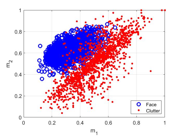
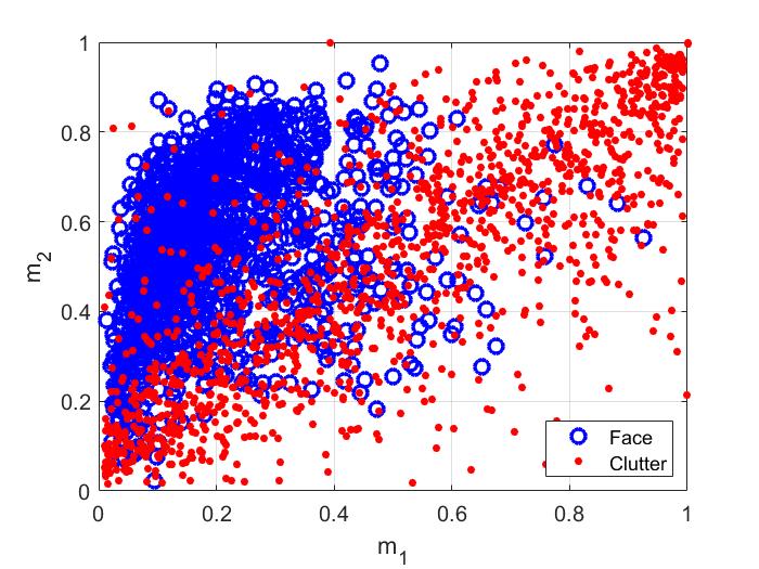
Figure 3: Three rectangular Haar-like filters imposed on some face and clutter images (up), and the distribution of mean measurement for the images (down).

The Haar-like features are local texture descriptors that measure differences in the average values of intensity in adjacent rectangular regions [23, 24]. Figure 3 illustrates some simple Haar-like features widely used in applications. The main advantage of Haar-like features is their calculation speed, facilitated by the use of integral images [25]. Viola and Jones, in [17], utilize these Haar-like features for face detection. In [26], a Haar-like feature detector was trained to identify stones on an SSS mosaic showing heterogeneous sediment distribution. A generalized Haar filter-based convolutional neural network is proposed in [27] for both vehicle and pedestrian detection. In [28], a smart cane function is developed by integrating face recognition features on the cane using Haar-like features and Eigenfaces. Additionally, in [29], an enhanced two-layer face detector composed of both Haar-like and Multi-Block Local Binary Pattern (MB-LBP) features is presented. In [30], a Haar-like local ternary co-occurrence pattern is designed for image retrieval applications. This pattern deploys four different Haar-like filters to capture directional information in the image. A vision-based hardware recognition architecture combining Haar-like feature extraction and support vector machine (SVM) classification is presented in [31]. In [32], the performance of three commonly used object detection approaches—Histogram of Oriented Gradients (HOG), Haar-like features, and Local Binary Pattern (LBP)—is investigated, and a robust detection algorithm is proposed using a combination of the three different feature descriptors and AdaBoost cascade classification. Experimental results from [32] show that LBP features outperform the other two feature types with a higher detection rate. In [33], a Haar-like descriptor based on the integral image and a multilayer perceptron type classifier is proposed. Experimental results show that the system inherits advantages of the Haar-like descriptor and artificial neural networks in terms of robustness and speed. Haar-like filters are also applied in deep convolutional neural networks (DCNN) for feature extraction [34, 35, 36]. Recently, Haar-like filters have been applied in several fields of classification, demonstrating their efficiency [37, 38, 39, 40, 41].

Although Haar-like features are significantly simple and efficient, they have some limitations in application [42, 43]. To enhance the capability of Haar-like features, various variations have been proposed, such as joint Haar-like features [23], rotated Haar-like features [44, 45], block difference features [46], and Haar-like features with disjoint rectangles [47, 48, 43]. Additionally, in [43], the Haar-like features are subjected to the application of differential evolution (DE), genetic algorithm (GA), and particle swarm optimization (PSO) to accelerate the Viola-Jones classifier. An extension of the Viola and Jones detection framework is presented in [47] by removing the geometry restriction of Haar-like features. The authors of [47] propose a richer representation called scattered rectangle features, which explore more orientations than horizontal, vertical, and diagonal Haar-like features. Also, a novel type of feature named Non-Adjacent Rectangle (NAR) Haar-like feature is introduced in [48] to characterize the co-occurrence between facial landmarks and their surroundings. Traditional Haar-like features and NAR Haar-like features are then combined in [48] to form more powerful representations.

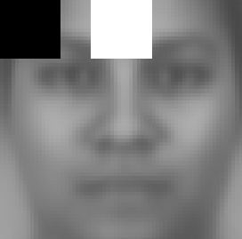
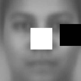
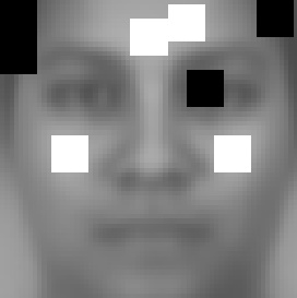
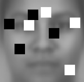
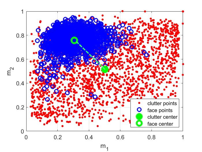
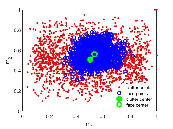
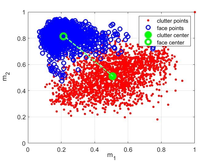
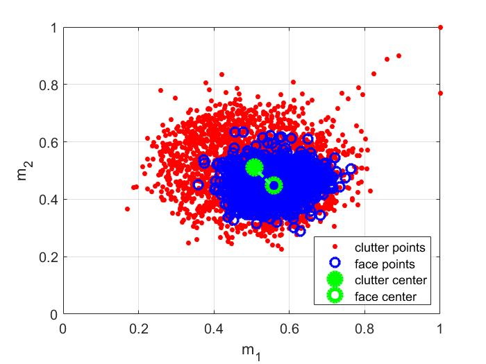
Figure 6: Graph of five disperse Haar-like filters and mean measurement of the images for them. The first and third filters satisfy Equation (3.5) but the second and forth ones do not. The third filter, which has bigger $s^{*}$, can separate face and clutter points better than the others.

A new type of Haar-like filter, called the dispersed Haar-like filter, is presented in [43], where the white and black parts of the filter are generally disjoint. To create this filter, a matrix is randomly evaluated with values of $1$, $0$, and $-1$ initially. Subsequently, the pixel values are optimized using optimization algorithms such as DE, GA, and PSO. The pixels evaluated as $1$ and $-1$ constitute the white and black parts of the filter, respectively, while pixels evaluated as $0$ do not participate in the filter. The non-adjacent rectangles assumed in [43] allow for more flexibility in the Haar-like filter, providing robust face detection. Some of these filters are shown in Figure 6. According to [43], these filters significantly improve detection rates for three reasons:

• Classical forms of Haar-like filters have a rigid structure, whereas the new filter has a flexible structure.

• The optimal structure of the new filter can be determined by optimization algorithms based on machine learning.

• There are dispersed dots in the filter that can extract local face features instead of only fixed global face features.

The study in this work delves into the analysis of the dispersed Haar-like filters, aiming to determine the optimal placement of white and black pixels within them. Given the necessity for these filters to extract crucial facial features, novel algorithms are introduced to achieve this goal without encountering issues of overfitting. This paper not only puts forth global filters but also introduces local variants. Furthermore, a composite algorithm is proposed for detecting faces ’in-the-wild’. The paper concludes with the presentation of experimental results that showcase the effectiveness of the new optimized Haar-like filters.

The subsequent sections of the paper are structured as follows: Section 2 offers an introduction to Haar-like filters. Following this, Section 3 introduces a class of the dispersed Haar-like filters, known for their simplicity in application and accuracy in classification. The proposed filters exhibit effective performance without succumbing to overfitting. The Overfitting, an undesirable behavior wherein filters capture details (or noises) more than generality, is addressed in Section 4. An algorithm is presented in this section to moderate the learning rate of the filters, preventing the overfitting. This idea is further extended in Section 5, where a local optimized dispersed Haar-like filter is proposed, focusing on the most important parts of the face. One can see that the accuracy of the local filter is comparable to that of the global one. Additional experimental results concerning the accuracy and efficiency of the new Haar-like filters are provided in Section 6. These results are further compared to the best ones obtained by the Viola-Jones algorithm. A classifier is proposed in this section which highlights the advantages of the optimally selected dispersed Haar-like filters over the Viola-Jones algorithm. Finally, the paper concludes with a brief summary presented in Section 7.

2 Haar-like filters

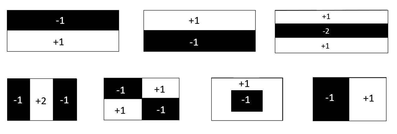
Figure 1: Some traditional Haar-like filters with their default weights marked on them.

Haar-like filters are extensions of two-dimensional Haar functions, widely employed in object detection [49]. As depicted in Figure 1, they are typically represented as two or several rectangular areas comprising black and white pixels [17]. Given their application in feature extraction, they are also referred to as Haar-like features in the literature [50]. One of the primary advantages of Haar-like filters is their simplicity, speed, and sufficient accuracy for classification [17]. Feature value $g$ for a Haar-like filter is defined as

$$g(\mathbf{x})=v_{1}\,m_{1}(\mathbf{x})+v_{2}\,m_{2}(\mathbf{x}),$$ (2.1)

Here, $\mathbf{x}$ represents an image, and $m_{1}$ and $m_{2}$ are the mean intensities of the pixels in the image restricted to the black and white regions, respectively. Additionally,are weights corresponding to the regions traditionally represented as two integers, where their sum is zero. Figure 1 illustrates various examples of Haar-like filters with default weights marked on their rectangles. In these examples, the weights are assigned as:

$$v_{1}=-1~{},~{}~{}~{}v_{2}=1.$$ (2.2)

This assignment holds true when the sizes of the black and white regions are equal. However, various algorithms exist to determine the optimal values of the weights, such as brute-force search (BFS) [17], genetic algorithms (GA) [51, 52, 53], and Fisher’s linear discriminant analysis (FLDA) [54]. Since this paper specifically concentrates on finding optimal Haar-like filters with equal black and white regions, the weights are considered as given in Equations (2.2).

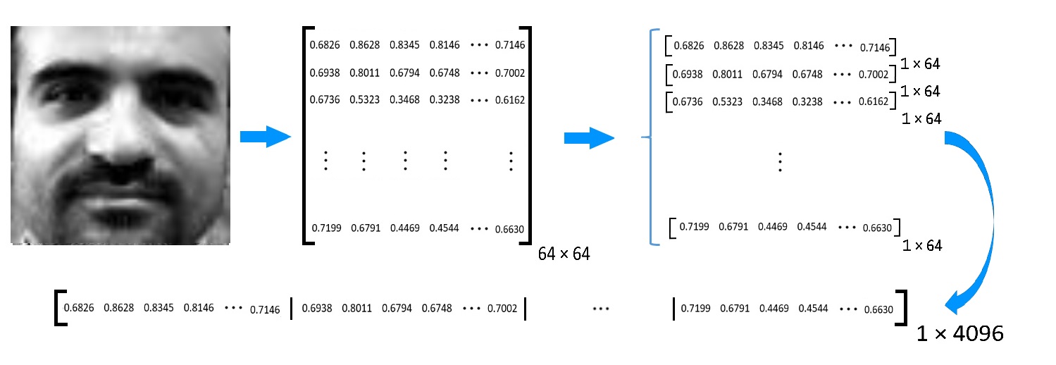
Figure 2: Vectorizing an image. An image $64\times 64$ is transformed to a row vector of length $4096$.

For simplicity, images in a dataset can be vectorized, as illustrated in Figure 2. Consequently, the black and white regions of a Haar-like filter can be represented by two vectors, $\mathbf{b}$ and $\mathbf{w}$, respectively, evaluated as:

$$\mathbf{b}(p)=\left\{\begin{array}[]{ll}1,&\hbox{if}~{}~{}p\in B,\\ 0,&\mbox{o.w.}\end{array}\right.,~{}~{}~{}~{}\mathbf{w}(p)=\left\{\begin{array}[]{ll}1,&\hbox{if}~{}~{}p\in W,\\ 0,&\mbox{o.w.}\end{array}\right.$$ (2.3)

in vector form, where $p$ varies from $1$ to the size of the vectorized image $\mathbf{x}$. Here, $B$ and $W$ denote the black and white regions of the filter, respectively. Then the feature value, $g$, can be expressed in vector form as

$$g(\mathbf{x})=v_{1}\,m_{1}(\mathbf{x})+v_{2}\,m_{2}(\mathbf{x})=[m_{1}(\mathbf{x}),m_{2}(\mathbf{x})].\,[v_{1},v_{2}]^{T},$$ (2.4)

where $m_{1}$ and $m_{2}$ are computed as

$$m_{1}(\mathbf{x}) =\frac{1}{N_{\mathbf{b}}}\mathbf{b}.\,\mathbf{x}^{T},~{}~{}~{}m_{2}(\mathbf{x})=\frac{1}{N_{\mathbf{w}}}\mathbf{w}.\,\mathbf{x}^{T}.$$ (2.5)

such that $N_{\mathbf{b}}$ and $N_{\mathbf{w}}$ are the numbers of pixels in black and white regions of the filter, respectively. Note that, $N_{\mathbf{b}}+N_{\mathbf{w}}$ represents the total number of engaged pixels in the filter, denoted by $N$. The superscript $T$ on vector $\mathbf{x}$ shows the transpose operator converts a row vector to a column one. To label image $\mathbf{x}$ as either the object or clutter, feature value $g$ is compared to threshold $\theta$, and the classification is performed by the classifier $h(\mathbf{x})$ as:

$$h(\mathbf{x})=\left\{\begin{array}[]{ll}+1~{}~{}(\hbox{or object})&\hbox{if}~{}g(\mathbf{x})>\theta,\\ -1~{}~{}(\hbox{or clutter})&\hbox{if}~{}g(\mathbf{x})<\theta.\end{array}\right.$$ (2.6)

Note that, the above equation can be abbreviated as

$$h(\mathbf{x})=sign(g(\mathbf{x})-\theta),$$

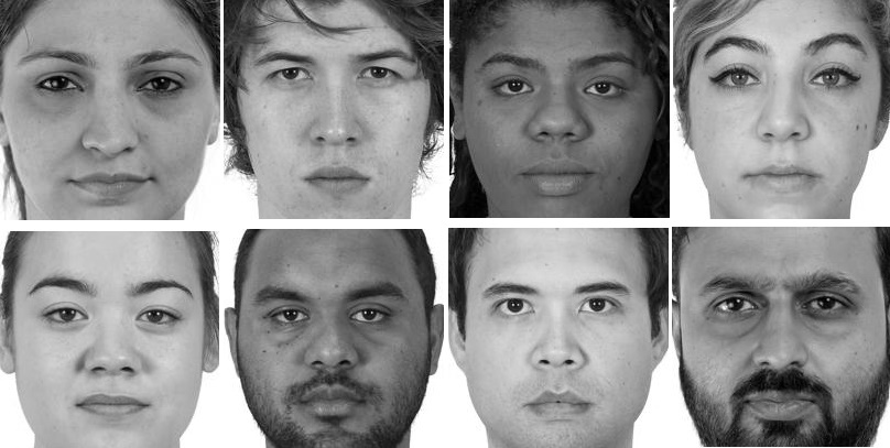
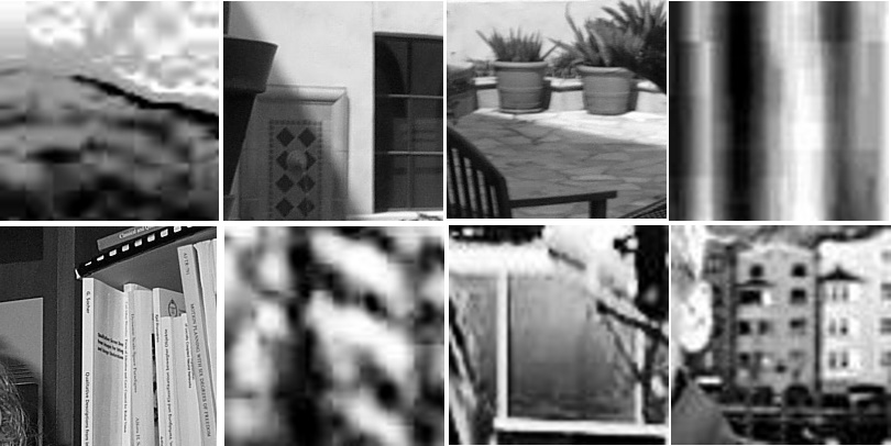
Figure 4: Some human frontal face (left) and clutter (right) images in the face and clutter databases, respectively.

where $sign(.)$ is a function that returns the sign of a real number. Traditional Haar-like filters are considered too simple, and various modifications have been proposed to enhance their performance, as documented in previous studies [23, 50, 43]. These modifications primarily vary in terms of orientation and the number of rectangles in relation to the template. In Figure 3, three rectangular Haar-like filters are depicted overlaying on facial and clutter images, along with the corresponding distribution of mean measurements $(m_{1},m_{2})$. The mean measurements of the images where already studied in [50]. For better visualization clarity, the number of rectangles in the Haar-like filters, depicted in Figure 3, is limited to three. The first Haar-like filter characterizes the intensity difference between the eyes and the region encompassing the bridge of the nose. The second descriptor gauges the intensity contrast between the corner of the hairline and the left side of the forehead. Finally, the third Haar-like filter measures the intensity difference between the eyes and the cheekbones area. The second row of Figure 3 is dedicated to the distribution of mean measurements for $1410$ face and $1410$ clutter images. The face images are sourced from databases CFD [55], CFD-MR [56], and CFD-INDIA [57], where the facial regions were manually cropped and resized to images of size $64\times 64$. This combined database is referred to as CFD-T in this paper. Additionally, the clutter images are extracted from a database that contains no human faces. Some representative face and clutter images from these databases are shown in Figure 4. The studied images are grayscale, and the light intensity of pixels in the images is normalized by dividing their values by $255$. The distribution of the intensity histogram of images is equalized using histogram equalizer function in Matlab software, named ’histeq’. Subsequently, $m_{1}$ and $m_{2}$ are calculated for the images, and their mean measurements are plotted in Figure 3. Similar to the methodology in [50], the points plotted on the $(m_{1},m_{2})$ graph corresponding to face and clutter images are referred to as face and clutter points, respectively, in this paper. From Figure 3, it is evident that the face points are predominantly distributed on top of the clutter points, irrespective of the type and size of the Haar-like filter. Furthermore, from the figure, it can be observed that the face points exhibit a high degree of correlation with each other, while the clutter points are generally spread out in the region.

3 dispersed Haar-like filters

Traditional Haar-like filters are constrained by some rectangular deadpan shapes. Several noteworthy papers [47, 48, 43] have explored Haar-like features based on disjoint rectangles. As mentioned in these papers, the use of disjoint rectangles offers more flexibility in face detection. It’s important to note that the separation of rectangles in Haar-like features allows disjoint areas to share their contributions in face detection, a feature not present in joined rectangles. In this section, we build upon the concept of disjoint Haar-like filters introduced in [43]. We propose an extreme case for a dispersed Haar-like filter efficiently disjoints face and clutter points in the $(m_{1},m_{2})$ graph.

3.1 fully dispersed Haar-like filters

In this section, we look for the best position of the Haar-like rectangles including human face features. Since the mean of the face images statistically is the best representation for the images, it may have the most important face features. Numerical experiments reveal that the mean of clutter images is also crucial for classification. Assume the face and clutter databases contain $N_{f}$ and $N_{c}$ vectorized face and clutter images of size $64\times 64$, respectively. Then each image is converted to a vector of size $1\times 4096$ after vectorization (see Figure 2). The mean values of the face and clutter images are computed as follows:

$$\mathbf{m}_{F}=\frac{1}{N_{f}}\sum_{i=1:N_{f}}\mathbf{f}_{i},~{}~{}~{}\mathbf{m}_{C}=\frac{1}{N_{c}}\sum_{i=1:N_{c}}\mathbf{c}_{i},$$ (3.1)

where $\mathbf{f}_{i}$ and $\mathbf{c}_{i}$ represent the $i$-th vectorized face and clutter images, respectively. One can see the image of $\mathbf{m}_{F}$ is also a face, while the image of $\mathbf{m}_{C}$ is a gray-scale neutral image with a light intensity of $0.5$ when the light is normalized between $0$ and $1$. If the black and white rectangles of a Haar-like filter are positioned over the corresponding black and white regions of the mean face image in a way that maximizes the feature value $g(\mathbf{m}_{F})$ then the maximum value of

$$m_{g_{F}} =\frac{1}{N_{f}}\sum_{i=1:N_{f}}g(\mathbf{f}_{i})=g(\frac{1}{N_{f}}\sum_{i=1:N_{f}}\mathbf{f}_{i})=g(\mathbf{m}_{F}).$$ (3.2)

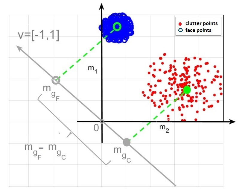
Figure 5: Graph of $m_{g_{F}}$ and $m_{g_{C}}$ for some face and clutter points where the weights are $-1$ and $1$ for the black and white regions, respectively.

is obtained. Here, $m_{g_{F}}$ represents the mean of feature values for the face images. From Equation (2.4), the value of $m_{g_{F}}$ can be interpreted as the length of the projection of vector $[m_{1}(\mathbf{m}_{F}),m_{2}(\mathbf{m}_{F})]$ on $[v_{1},v_{2}]$. Consequently, as $m_{g_{F}}$ increases, the face points in the $(m_{1},m_{2})$ graph are shifted toward the left-top corner. The graphical representation of the relationship between $m_{g_{F}}$ and the mean measurement of the face images is depicted in Figure 5. Similar relationships can be established for the mean measurements of the clutter images, with the aim of shifting them towards the right-down corner in the $(m_{1},m_{2})$ graph by decreasing the mean value of $g$ for them. If the black and white rectangles of a Haar-like feature are arranged such that $g(\mathbf{m}_{C})$ is minimized, then the mean value of $g$ for the clutter images, denoted by $m_{g_{C}}$, is also minimized. This is because:

$$m_{g_{C}}=\frac{1}{N_{c}}\sum_{i=1:N_{c}}g(\mathbf{c}_{i})=g(\frac{1}{N_{c}}\sum_{i=1:N_{c}}\mathbf{c}_{i})=g(\mathbf{m}_{C}).$$ (3.3)

From Equation (3.3), $m_{g_{C}}$ is the projection of vector $[m_{1}(\mathbf{m}_{C}),m_{2}(\mathbf{m}_{C})]$ on $[v_{1},v_{2}]$. Figure 5 graphically illustrates $m_{g_{C}}$ for vector $\mathbf{v}=[-1,1]$. It’s worth noting that the relationships described are applicable for any coefficient vector $\mathbf{v}=[v_{1},v_{2}]$ employed in linear discriminant analysis [54]. It is worth noting that the classifier $h$ performs better when the Haar-like filter is configured to maximize $m_{g_{F}}$ and minimize $m_{g_{C}}$ simultaneously. This is equivalent to maximizing $m_{g_{F}}-m_{g_{C}}$. In this scenario, the distance between the mean values $m_{g_{F}}$ and $m_{g_{C}}$ is maximized, leading to better discrimination between face and clutter images. To achieve this goal, it is sufficient to define a new vector

$$\mathbf{m}_{F_{C}}=\mathbf{m}_{F}-\mathbf{m}_{C},$$ (3.4)

and find a Haar-like filter such that minimizes $g(\mathbf{m}_{FC}).$ Therefore, since

$$s^{*} =\max\{g(\mathbf{m}_{FC})\}$$ (3.5)

$$=\max\{g(\mathbf{m}_{F})-g(\mathbf{m}_{C})\}$$

$$=\max\{\frac{1}{N_{f}}\sum_{i=1:N_{f}}g(\mathbf{f}_{i})-\frac{1}{N_{c}}\sum_{i=1:N_{c}}g(\mathbf{c}_{i})\}$$

$$=\max\,\{m_{g_{F}}-m_{g_{C}}\},$$

the distance between $m_{g_{F}}$ and $m_{g_{C}}$ is maximized when $g(\mathbf{m}_{FC})$ is maximized. Five Haar-like filters and the mean measurements of the face and clutter images corresponding to these filters are illustrated in Figure 6. The first and third filters satisfy Equation (3.5), while the second and fourth ones do not. The first and second Haar-like filters contain two disjoint blocks, a black and a white.

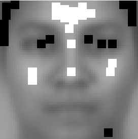
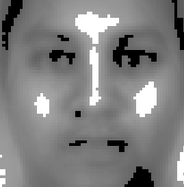
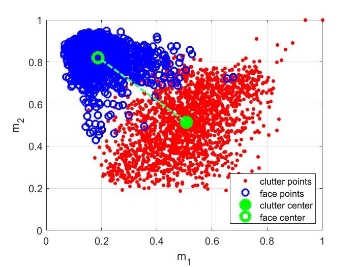
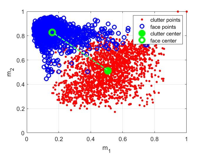
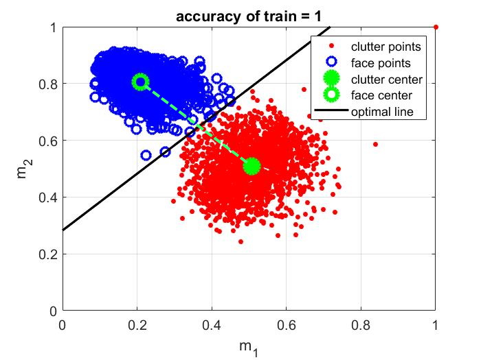
Figure 7: First column: image of a Haar-like filter satisfying Equation (3.5) with $32$ blocks of size $4\times 4$, and mean measurement of the face and clutter points respect to it. Second column: image of a full dispersed Haar-like filter obtained by Algorithm 1 and the mean measurement of the images respect to it. Third column: image of a full dispersed Haar-like filter obtained by Algorithm 2 and the mean measurement of the images respect to it. The third filter separates the face and clutter points, linearly, but the other ones do not.

From Figure 6, it is evident that the first filter pushes the face points toward the left-top corner in the $(m_{1},m_{2})$ graph more effectively than the second one. This observation remains valid for Haar-like filters with more blocks. In comparing the third and fourth filters, each composed of eight blocks, it becomes evident that the third one significantly outperforms the fourth one in separating face and clutter points. Additionally, the third filter achieves a better separation of face and clutter points compared to the first filter. This effect reveals that Haar-like filters with finer blocks, resulting in larger $s^{*}$, lead to better classifiers. A Haar-like filter with $32$ blocks satisfying Equation (3.5) is presented in Figure 7. Comparing Figure 6 and Figure 7, it is evident that the last filter produces better results compared to the previous ones with fewer blocks. Each block in the last filter consists of $4$ pixels. Furthermore, The number of blocks can be increased up to the size of the filter if the blocks are shrunk to the pixels. Then, the blocks are replaced by the pixels in the filter in this situation. These replacements conclude the best Haar-like filter that one can find to disjoint face and clutter points. This filter is named fully dispersed Haar-like filter in this paper. Two fully dispersed Haar-like filters based on the CFD-T dataset are shown in Figure 7 for $N_{\mathbf{b}}=N_{\mathbf{w}}=256$ when the size of face and clutter images is $64\times 64$. These filters consist of $N=512$ pixels. The first filter is obtained when the mean of face and clutter images is calculated normally, as presented in Equation (3.1). It reveals that the left-top and right-top corners of a human head and its forehead are the most important black and white features for face images, respectively. It also indicates that eyes, cheeks, nose bridge, and the left side of the neck are important face features, although not as crucial as the previous ones, as they have less contribution in the filter. The mean measurements of the face and clutter images are shown in the second row of Figure 7. It is noteworthy that the filter can be easily constructed by sorting the pixels of the vector $\mathbf{m}_{FC}$ according to light intensity and selecting $256$ lower and $256$ upper ones as the black and white regions of the filter, respectively. The following algorithm outlines the process of creating the filter in Matlab software.

Algorithm 1 Making a fully dispersed Haar-like filter.

define $\mathbf{m}_{FC}$ as Equation (3.4)

define $N_{\mathbf{b}},N_{\mathbf{w}}$ and $N=N_{\mathbf{b}}+N_{\mathbf{w}}$

initialize $\mathbf{b}$ and $\mathbf{w}$ as zero vectors of size $\mathbf{m}_{FC}$

[$\mathbf{r}$, $\mathbf{o}$]=sort($\mathbf{m}_{FC}$)

$\mathbf{b}$($\mathbf{o}$(1:$N_{\mathbf{b}}$))=1

$\mathbf{w}$($\mathbf{o}$(end-$N_{\mathbf{w}}$:end))=1

From Figure 7, a fully dispersed Haar-like filter shifts face points toward the left-top corner, while it predominantly gathers clutter points around $(0.5,0.5)$ in the $(m_{1},m_{2})$ graph.Also, from Figure 6 and Figure 7, it is evident that the within-class variance of clutter points decreases as the number of blocks increases. This is trivial because the considered Haar-like features are concentrated only on two locations when one uses a filter with two blocks, but they are distributed over the image when the number of blocks increases. Consequently, the fully dispersed Haar-like filter clusters face and clutter points more effectively in the $(m_{1},m_{2})$ graph than the others.

3.2 Optimal fully dispersed Haar-like filters

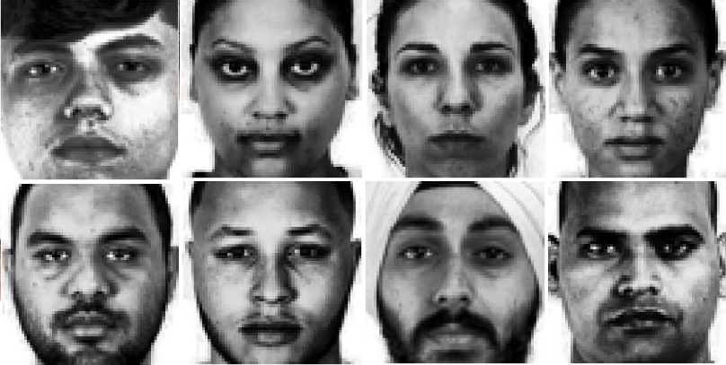
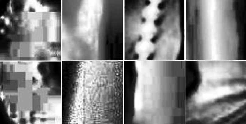
Figure 8: Some miss classified face (left) and clutter (right) images when the fully dispersed Haar-like filter obtained by Algorithm 1 is applied.

Now, there is an important question: Can one distribute pixels of a fully dispersed Haar-like filter more efficiently over the image? This optimization would result in less within-class variance of face and clutter points, leading to more accurate classification. To optimize the filter, more delicate features should be extracted from the images and appended to the filter. The sought features aim to decrease variances, particularly by incorporating features shared with misclassified images. It is important to note that the classifier (2.6) classifies images with the optimal value of $\theta$ to minimize the classification error for the Haar-like filter. Some misclassified face and clutter images are presented in Figure 8 when the Haar-like filter, obtained by Algorithm 1, is applied. From Figure 8, it is observed that the misclassified face images have white left-top and right-top corners, and some of them exhibit beards around their mouths. The impact of misclassified images can be amplified by using weighted summations

$$\mathbf{m}_{F}=\sum_{i=1:N_{f}}w^{f}_{i}\mathbf{f}_{i}~{},~{}~{}~{}\mathbf{m}_{C}=\sum_{i=1:N_{c}}w^{c}_{i}\mathbf{c}_{i}~{},$$ (3.6)

instead of the mean values, where $w^{f}_{i}\geq 0,w^{c}_{i}\geq 0,\sum_{i=1:N_{f}}w^{f}_{i}=1,\sum_{i=1:N_{c}}w^{c}_{i}=1,$ and higher weights are considered for the miss classified images. This leads removing the top corners from the Haar-like filter and adding a mouth to it when the misclassified images are amplified in (3.6). An optimized dispersed Haar-like filter is presented in the right column of Figure 7. The new filter is obtained using Algorithm 2, where the weights of the summations are updated inductively. From the mean measurement with respect to the new filter, as presented in Figure 7, the face and clutter points are linearly disjointed by the filter. This shows that the weighted summations (3.6) are significantly more efficient than the mean values (3.4), provided that the weight vectors $\mathbf{w}^{f}=[w^{f}_{1},w^{f}_{2},...,w^{f}_{N_{f}}]$ and $\mathbf{w}^{c}=[w^{c}_{1},w^{c}_{2},...,w^{c}_{N_{c}}]$ are appropriately selected. The weights in Algorithm 2 are updated according to:

$$w^{f/c}_{i}\leftarrow\begin{cases}w^{f/c}_{i}+1&\quad\text{if face/clutter image }\mathbf{x}_{i}\text{ is classified incorrectly}\\ w^{f/c}_{i}&\quad\text{o.w.}\end{cases}$$ (3.7)

iteratively for trial image $\mathbf{x}_{i}$. To perform this update, we can also use $hardlim$ function as:

$$w_{i}^{f} \leftarrow w_{i}^{f}+hardlim(-y_{i}),$$ (3.8)

$$w_{i}^{c} \leftarrow w_{i}^{c}+hardlim(~{}y_{i}~{}),$$ (3.9)

where $y_{i}=g(\mathbf{x}_{i})-\theta$. After updating the weights, we normalize them by dividing each to their summation as:

$$w^{f}_{i}\leftarrow w^{f}_{i}/(\sum_{i=1:N_{f}}w^{f}_{i})~{}~{}~{}~{}~{},~{}~{}~{}~{}~{}w^{c}_{i}\leftarrow w^{c}_{i}/(\sum_{i=1:N_{c}}w^{c}_{i}).$$ (3.10)

Algorithm 2 The algorithm to find the best weights for the face and clutter images.

define face vector $\mathbf{f}_{i}$ and initialize $w^{f}_{i}=1/{N_{f}}$ for $i=1,2,...,N_{f}$

define clutter vector $\mathbf{c}_{i}$ and initialize $w^{c}_{i}=1/{N_{c}}$ for $i=1,2,...,N_{c}$

define $\mathbf{m}_{F}$ and $\mathbf{m}_{C}$ as are presented in (3.6)

set $\mathbf{m}_{FC}=\mathbf{m}_{F}-\mathbf{m}_{C}$

find vectors $\mathbf{b}$ and $\mathbf{w}$ by Algorithm 1

find error of classifier $h$ presented in Eq. (2.6)

while error of the classification is not zero do

     ** update the weights as (3.8) and (3.9) **

     normalize the weights as (3.10)

     update $\mathbf{m}_{F}$ and $\mathbf{m}_{C}$ as are presented in (3.6)

     update $\mathbf{m}_{FC}$ as $\mathbf{m}_{FC}=\mathbf{m}_{F}-\mathbf{m}_{C}$

     find new vectors $\mathbf{b}$ and $\mathbf{w}$ by Algorithm 1

     find error of classifier $h$ presented in Eq. (2.6)

end while

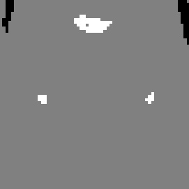
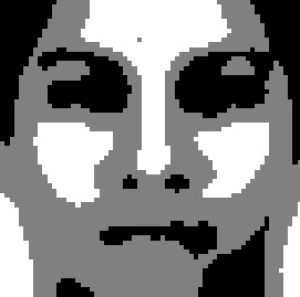
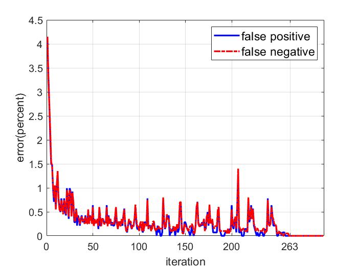
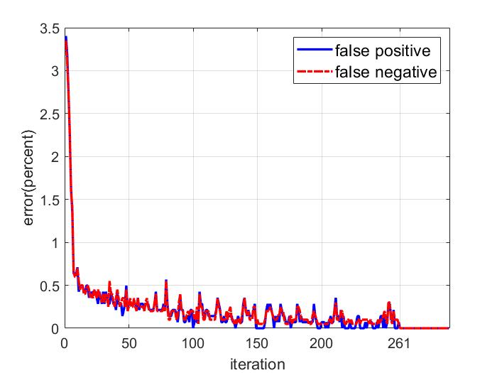
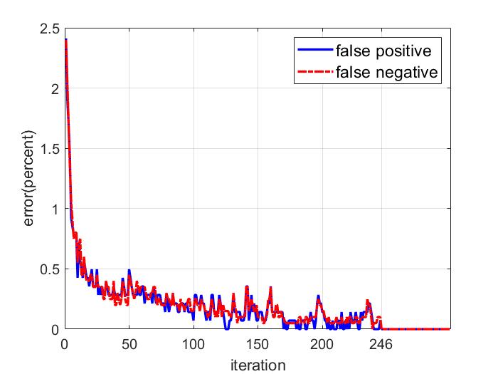
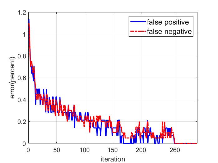
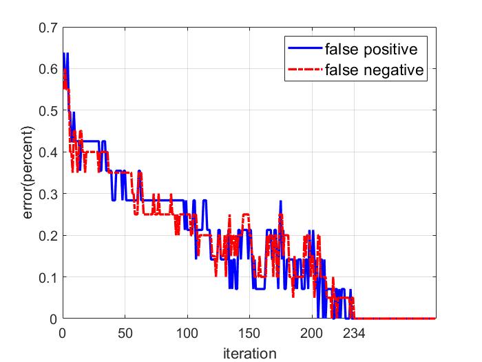
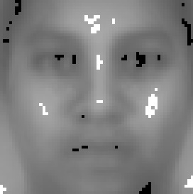
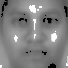
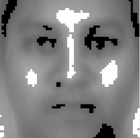
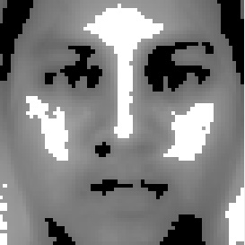
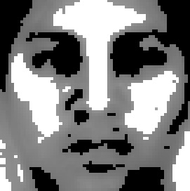
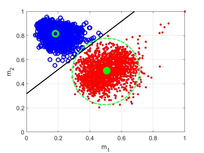
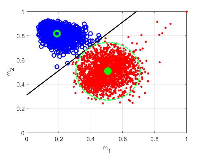
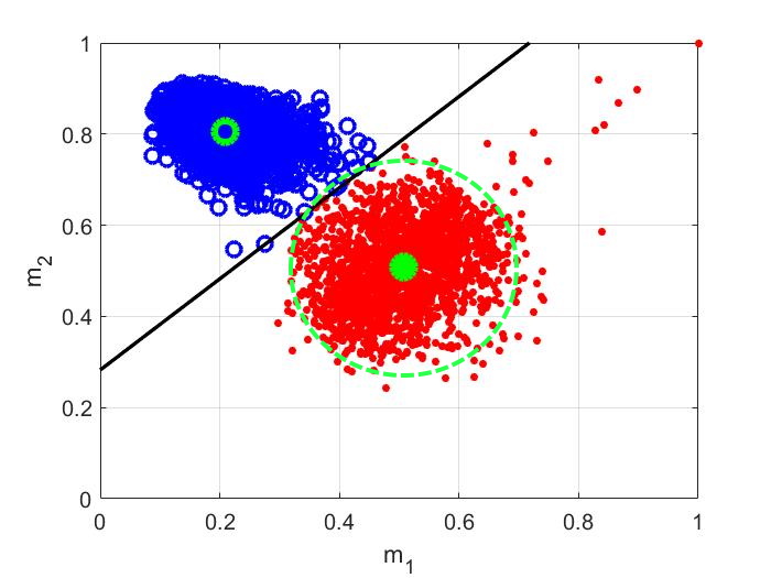
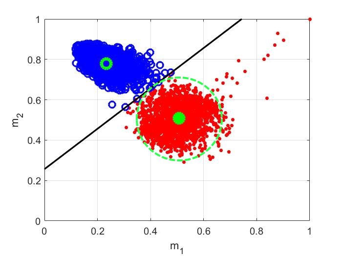
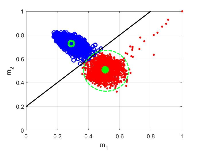
Figure 9: Numerical results of Algorithm 2 for five fully dispersed Haar-like firsts. The first row is dedicated to the initial filter. The second row is devoted to the value of false positive and false negative errors of classifier $h$ in field of each iteration of Algorithm 2. The third row shows the final filter. The mean measurement of the images for the final filter is shown in the fourth row. Size of the filters is $N=128,256,512,1024$ and $2048$ for the first, second, third, forth and fifth columns, respectively. From the forth row of this figure, the optimized filters disjoint face and clutter images, linearly.

The false positive and false negative errors of the classifier $h$, presented in Algorithm 2, are indicated in Figure 9 for some iterations. From the figure, it is observed that the errors decrease from $2.5$ to $0$ after $246$ iterations when the total number of engaged pixels in the filter is $N=256$. The errors for fully dispersed Haar-like filters of different sizes are also reported in Figure 9. From this figure, it is evident that the errors vanish after at most $300$ iterations when $N$ varies from $128$ to $2048$. Thus, the Haar-like filters linearly disjoint face and clutter points after at most $300$ times updating the weights. Notably, initial values of the errors are smaller for larger filters, indicating that larger filters capture more face features. Additionally, from Figure 9, the final filters focus on the same features when the size of filters is larger than or equal to $N=512$. It is advised not to use filters with less than or equal to $N=128$ pixels for face detection, as they are very sensitive to preprocessing and may not effectively capture face features in the presence of noise in the data. Note that the within-class variance is high when the size of the filter is very small, and the between-class variance is low if the size is too large. Therefore, it is advisable to use filters with moderate sizes, i.e., $N=256,512$ and $1024$ when the size of trial image is $64\times 64$.

Note that the same approach can be applied to dispersed Haar-like filters with multiple blocks, as shown in Figure 6, to find the optimal location of their rectangles. However, Algorithm 1 does not perform well for them, and a new, more complicated algorithm is required. Additionally, as mentioned in the previous subsection, filters with multiple blocks capture Haar-like features less effectively than fully dispersed ones where their pixels can freely move in the region. Therefore, we will only focus on fully dispersed filters and omit the consideration of filters with multiple blocks from this point forward.

4 Treating overfitting

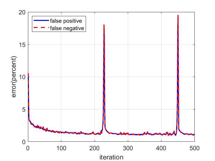
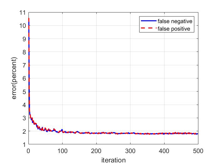
Figure 10: Images of two fully dispersed Haar-like filters and the curves of their errors. The first and third images depict the filters obtained by Algorithm 2 and Algorithm 3, respectively. The second and fourth images illustrate the errors of classification with respect to the iterations of Algorithm 2 and Algorithm 3, respectively. There are some jumps in the second image, indicating overfitting in the first filter.

Numerical experiments reveal that Algorithm 2 is not perfect for face feature extraction when the number of data is larger than $10,000$. In such cases, pixels of the dispersed Haar-like filter may be distributed separately over the region without effectively capturing valuable face features. This issue may arise when the pixels of the filter move freely on the region to minimize the classification error, and the minimization heavily depends on some miss-classified images containing some noises. Consequently, the noises may be retained by the filter instead of the features, especially when some miss-classified images are amplified several times. In this situation, we say that overfitting has occurred for the filter. Figure 10 displays images of two fully dispersed Haar-like filters trained on a dataset containing more than $20,000$ images, with over $9,000$ face and $11,000$ clutter images. The face images were collected from publicly available facial image datasets such as UTKFace and CDF-T (B-Datasets) [58]. The first filter in Figure 10 exhibits overfitting, while the second one does not. The pixels of the first filter are dispersed widely across the region, while they are predominantly located on the face features for the second filter. The first filter is obtained from Algorithm 2 after $500$ iterations. False positive and false negative errors of the classifier $h$, as presented in Algorithm 2, are illustrated in Figure 10 for several iterations. Notably, the errors increase suddenly at two iterations, indicating the filter learns some noises during training. The final filter is not efficient, and we need to modify it by modifying Algorithm 2. The previous algorithm can be improved by replacing the sigmoid function

$$sigmoid(y)=1/(1+\exp(-\epsilon y)),$$

instead of the $hardlim$. In this situation updates (3.8) and (3.9) are replaced by

$$w_{i}^{f} \leftarrow w_{i}^{f}+sigmoid(-y_{i}),$$ (4.1)

$$w_{i}^{c} \leftarrow w_{i}^{c}+sigmoid(~{}y_{i}~{}),$$ (4.2)

in the new algorithm. The sigmoid function has a shape parameter, denoted by $\epsilon$, which governs the function’s shape [59]. The function is $1/2$ for $\epsilon=0$ and $hardlim(y)$ for $\epsilon=\infty$. Therefore, Algorithm 3 is proposed in this section to treat the overfitting. The final Haar-like filter of the algorithm is presented in Figure 10, where the shape parameter is set to $\epsilon=20$. The errors of the new algorithm, as shown in Figure 10, exhibit no undesirable jumps, indicating the absence of overfitting.

Algorithm 3 The algorithm to find the best weights of data without over-fitting.

define face vector $\mathbf{f}_{i}$ and initialize $w^{f}_{i}=1/{N_{f}}$ for $i=1,2,...,N_{f}$

define clutter vector $\mathbf{c}_{i}$ and initialize $w^{c}_{i}=1/{N_{c}}$ for $i=1,2,...,N_{c}$

define $\mathbf{m}_{F}$ and $\mathbf{m}_{C}$ as are presented in (3.6)

set $\mathbf{m}_{FC}=\mathbf{m}_{F}-\mathbf{m}_{C}$

find vectors $\mathbf{b}$ and $\mathbf{w}$ by Algorithm 1

find error of classifier $h$ presented in Eq. (2.6)

initialize shape parameter $\epsilon$.

while error of the classification is not zero do

     ** update the weights as (4.1) and (4.2) **

     normalize the weights as (3.10)

     update $\mathbf{m}_{F}$ and $\mathbf{m}_{C}$ as are presented in (3.6)

     update $\mathbf{m}_{FC}$ as $\mathbf{m}_{FC}=\mathbf{m}_{F}-\mathbf{m}_{C}$

     find new vectors $\mathbf{b}$ and $\mathbf{w}$ by Algorithm 1

     find error of classifier $h$ presented in Eq. (2.6)

end while

5 Local dispersed Haar-like filters

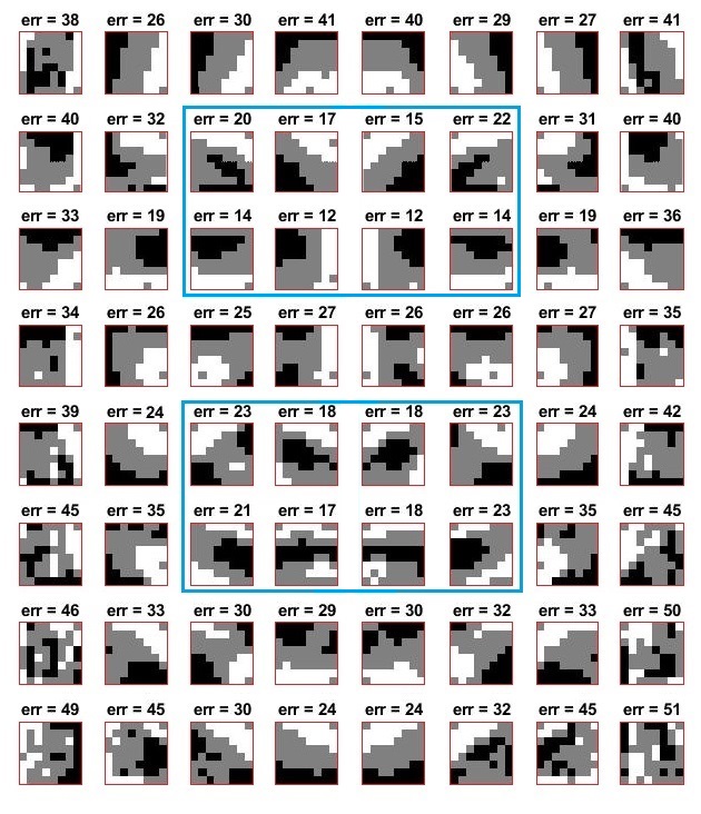
Figure 11: 64 local dispersed Haar-like filters for face feature extraction. Those filters containing the eyes, eyebrows, nose, and mouth extract more Haar-like features, leading to more accurate results. The classification error for these filters is less than or equal to $23\%$. The border filters provide less accurate results as they mainly contain noise.

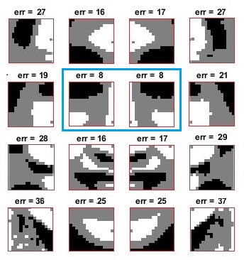
Figure 12: 16 local dispersed Haar-like filters for face feature extraction. Filters containing eyes, nose, and cheeks extract more important features of the face, leading to more accurate results with an $8\%$ classification error. Following those, filters containing the forehead and mouth are also crucial, resulting in less than $18\%$ classification error. However, corner filters provide less accurate results as they mainly contain noise.

Local dispersed Haar-like filters can also be obtained using Algorithm 3. These local filters tend to yield improved results when a part of a face image is damaged or noisy. The local filters are displayed in Figure 11 and Figure 12 for analysis, where the image is partitioned into $64$ and $16$ parts, respectively. Classification errors corresponding to the local filters are displayed on top of them. It is evident that the error varies from $12\%$ to $51\%$ in Figure 11, while in Figure 12, it ranges from $8\%$ to $39\%$. Notably, the central filters around the eyes exhibit more accurate results, while the border ones have less accuracy, as depicted in the figures. Moreover, corner filters, which encompass the background of face images, exhibit the highest error values. It should be noted that the effectiveness of local filters decreases when they become small, especially when the size of the test image is also small. Therefore, it is advisable to utilize sufficiently large local filters to effectively capture Haar-like features locally. These sufficiently large local filters are referred to as semi-local filters, here.

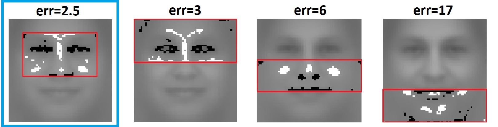
Figure 13: Four semi-local Haar-like filters obtained by Algorithm 3. Errors of the classification respect to the filters, presented on top of them, reveal the first filter extracts Haar-like face features more efficient than the others.

The local filters presented in Figures 11 and 12 motivate the definition of a new semi-local filter that encompasses eyes, eyebrows, nose and cheeks to more efficiently capture Haar-like features of the face. The proposed semi-local filter is displayed in the first column of Figure 13. Three additional semi-local filters are also presented in Figure 13, applied to the top, middle, and bottom parts of the images. Obtained through Algorithm 3, the errors of classification with respect to the semi-local filters are displayed in Figure 13. The results demonstrate that the semi-local filters reduce false positive and false negative errors to $2.5\%$, $3\%$, $6\%$, and $17\%$, respectively, after $400$ iterations. Given the higher accuracy of the proposed semi-local filter compared to the others, it is evident that the filter captures more face features, as expected. It must be noted that the optimized global dispersed Haar-like filter, presented in the previous section, results in $2\%$ error. This indicates that the first semi-local filter performs as well as the global one, and it can be used as a substitute, reducing computational cost. Notably, the second semi-local filter also achieves high accuracy by including the eyes and the surrounding region. However, the accuracy is notably reduced for the fourth filter due to the presence of noise. Variations in facial features, such as the presence or absence of a beard, can act as noise for the fourth filter, leading to a significant reduction in accuracy.

6 Experimental results

In this section, we begin by applying the Haar-like filter obtained through Algorithm 3 to face detection across various datasets. The algorithm is trained on $70\%$ of a dataset and tested on the remaining $30\%$ to assess its accuracy. Subsequently, a new algorithm is introduced that uses global Haar-like filters obtained through Algorithm 3 to detect human faces ”in the wild.” The accuracy of the new algorithm depends significantly on the preprocessing steps, and its effectiveness in different scenarios is discussed in this section. The results are compared to the best outcomes achieved by the Viola-Jones algorithm, yielding some noteworthy conclusions.

6.1 Case study 1

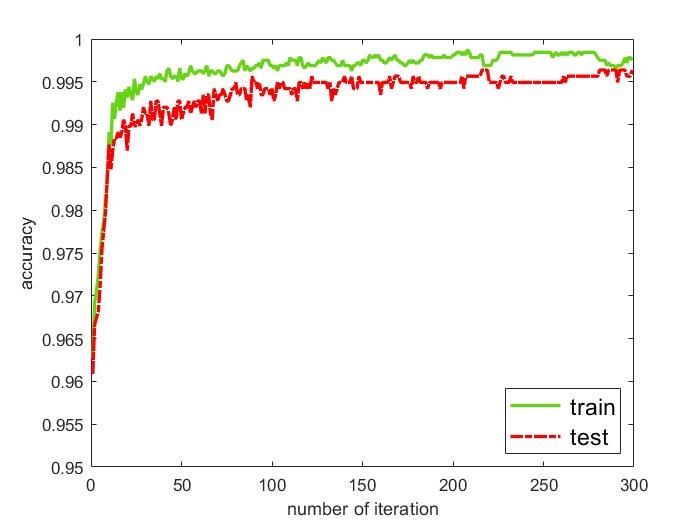
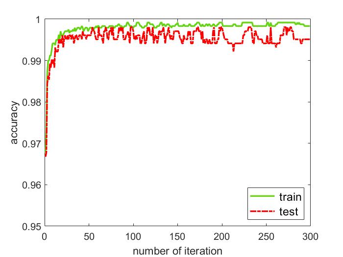
Figure 14: Accuracy of Algorithm 3 in each iteration applied on Datasets AR (left) and CF (right). The accuracy is more than $99\%$ when the iterations are more than $200$.

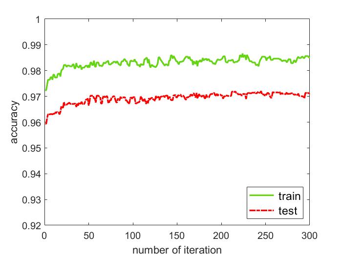
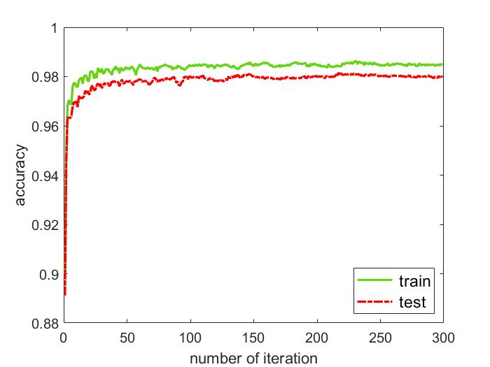
Figure 15: Accuracy of Algorithm 3 in each iteration applied on Datasets MIT (left) and UTK (right). The accuracy is less than $97\%$ and $98\%$ for MIT and UTK datasets, respectively.

Consider the AR Dataset [58] for face images. Algorithm 3 is employed to generate an OPB Haar-like filter and perform image classification. In Figure 14 (left), the accuracy of the classification is reported for each iteration of the algorithm. The error is smaller than $1\%$ for test images when the number of iterations exceeds $200$. Similar results are also obtained for the CF dataset, as shown in Figure 14 (right). The images in AR and CF datasets have high resolution, and they are reshaped to $64\times 64$ before feature extraction. Then, a dispersed Haar-like filter with $N=512$ engaged pixels is applied for the classification in Algorithm 3. Due to the sufficiently large size of the images, OPB Haar-like filters successfully extract facial features, resulting in accurate recognition of face images. However, the accuracy of the algorithm decreases when the resolution of trial images is lower. For example, the accuracy of the algorithm is less than $97\%$ when the MIT dataset is used for feature extraction. The size of images in the dataset is $19\times 19$. Figure 15 (left) shows the accuracy of Algorithm 3 for this dataset. The results, as depicted in Figure 15 (left), are not sufficiently accurate. Furthermore, as seen in Figure 14, the numerical results of Algorithm 3 for AR and CF datasets exhibit some small jumps in certain iterations, indicating a lack of strong stability in the results. To improve stability, it is beneficial to enrich the databases with more images. In such a scenario, the algorithm focuses solely on more general features while ignoring the noise in the data. Figure 15 (right) displays the accuracy of the algorithm concerning the UTK dataset, which includes more than $10,000$ images. It is notable thatthe AR and CF datasets include approximately $2000$ and $1400$ images, respectively. As shown in Figure 15 (right), the algorithm’s results are stable without jumps for iterations beyond $200$. However, this stability might result in slightly reduced accuracy. Comparing Figure 14 and Figure 15 (right), one can observe a decrease in accuracy for the UTK dataset compared to the AR and CF datasets. The accuracy is approximately $98\%$ for the UTK dataset, whereas it is over $99\%$ for the AR and CF datasets.

6.2 Case study 2

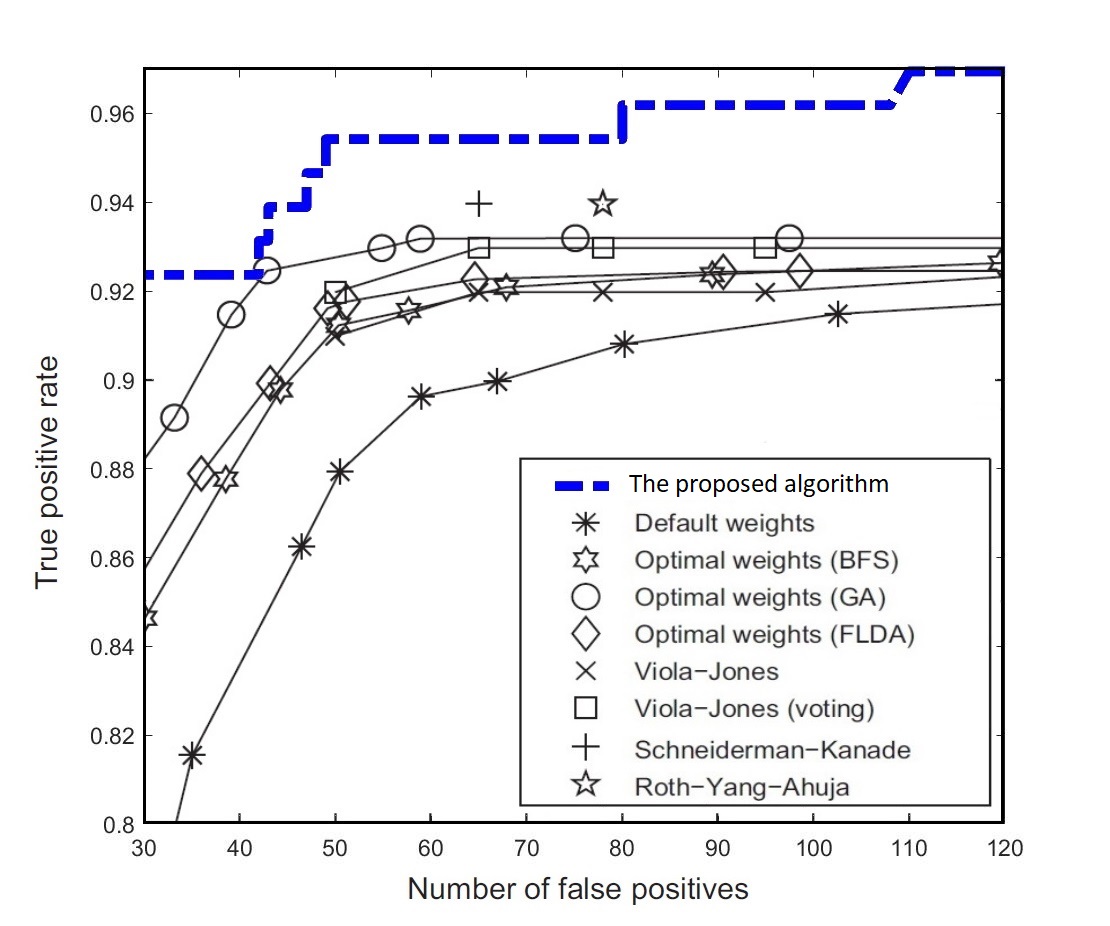
Figure 16: Roc curve for some face detector algorithms. The proposed algorithm is significantly more efficient than the others.

The face detection is performed on the MIT + CMU dataset [60], as considered in five other popular face detection methods presented in [43]. In [60], a simple neural network is utilized to learn face and clutter images. In [61], a new SNoW-based face detector is applied to the images, and the authors of [62] propose a probabilistic method to detect face images based on local appearance and principal component analysis (PCA). The results reported in [62] are based on evaluating a detector on 125 images from the MIT + CMU dataset. ROC curves of the methods are presented in Figure 16. Viola and Jones [17] results also are reported in Figure 16. The Viola and Jones detector had a cascade structure with $38$ nodes, which in turn is built using Haar-like features with default weights. A modest improvement also is done on Viola and Jones detector by using a simple majority voting scheme where each test image are evaluated using three different detectors. The ROC curves presented in Figure 16 obtained for default weights and those reported in [17] differ because of different datasets and different training process. The datasets used in [17] are not publicly available and the ROC curve in [43] is used for report. Note that, parameters such as how big the rectangles of Haar-like filters are used are not specified in [17] which makes it difficult to recreate the filters.

The ROC curve of the dispersed Haar-like filter obtained by Algorithm 3 is also reported in Figure 16. From this figure, the new Haar-like filter has better results compared to the other methods. In a special case, the proposed Haar-like filter is more accurate than the Viola and Jones method, which contains a combination of several Haar-like filters with some optimized weights. This suggests that the proposed Haar-like filter may be the simplest and the most accurate Haar-like filter which one can use for face detection.

6.3 Case study 3

In this section, the proposed dispersed Haar-like filters are applied for face detection ’in-the-wild’. The filters are trained using the CFD-T dataset, which is composed of CFD, MR, and INDI datasets. Subsequently, three global dispersed Haar-like filters are obtained using Algorithm 3, as shown in Figure 10. These filters are then utilized in the following algorithm.

Algorithm 4 The composed algorithm for face detection ’in-the-wild’.

input a test image $\mathbf{x}$ from a picture

do some preprocessing on $\mathbf{x}$

for $N=256,512$ and $1024$ do

     find a Haar-like filter and optimal value $\theta$ satisfying Eq. (2.6) by Algorithm 3.

     compute $h_{N}=sign(g(\mathbf{x})-\theta)$ for the filter

end for

define $h=\min\{h_{256},h_{512},h_{1024}\}.$

if $h==1$ then

     $\mathbf{x}$ is a face image

else

     $\mathbf{x}$ is a clutter image

end if

Algorithm 4 is a composite algorithm that makes a final decision by considering the decision of classifier (2.6) for the global filters. In this algorithm, a test image is classified as a face only if it is verified by three global decision functions. The new algorithm is referred to the composed algorithm, and it is designed to reduce false positive errors versus the previous ones. Note that, in a real case study, the majority of test images fed into the algorithm are likely to be clutter images, resulting in a high number of misclassified clutters. The composed algorithm is designed to minimize false positive errors by emphasis on them more than the false negative ones. To further reduce false positive errors, an experimental criterion is designed too. An image $\mathbf{x}$ detected as a face by Algorithm 4 is considered acceptable only if the positive decision remains consistent across several images in its vicinity. Since Haar-like filters are not sensitive to the details of an image, this trick works well, as we will demonstrate in the upcoming case studies.

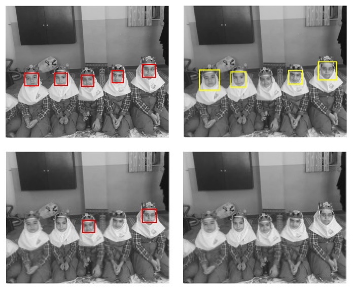
Figure 17: A picture with medium and low resolutions is presented in the first and second rows, respectively. Faces detected by the proposed and Viola-Jones algorithms are denoted by red and yellow squares, respectively. The proposed algorithm is able to detect face images more effectively.

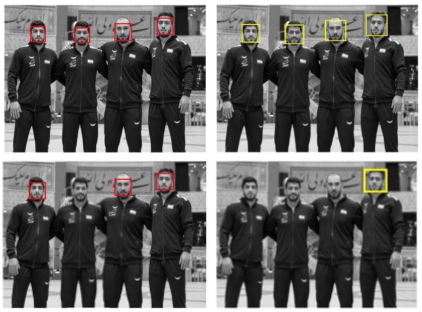
Figure 18: A picture with medium and low resolutions is presented in the first and second rows, respectively. Faces detected by the proposed and Viola-Jones algorithms are denoted by red and yellow squares, respectively. The proposed algorithm is able to detect face images more effectively.

For face detection ’in-the-wild’, we employ the idea presented in [63] to recognize the skin region in a picture. This significantly reduces the computational cost. The transformation matrix introduced in [63] is expanded here for larger regions to better distinguish the skin region. Therefore, square frames of the picture including the skin region are inserted into Algorithm 4 as test images. Although in Algorithm 4 a test image is labelled as a human face if the decision function $h$ equals $1$, a face decision is experimentally verified only if $h=1$ for some adjacent frames, as mentioned before. The number of adjacent frames verifying the face detection depends on the size of frames, and we assume $2\%$ of it in this research. In Figure 17, a picture is shown including five human faces. The size of the picture is considered as $400\times 400$ and $200\times 200$. The face images distinguished in the picture are denoted by red rectangles. As one can see, the proposed algorithm detects face images correctly without any errors. The Viola-Jones algorithm of the Matlab software is also applied to extract the faces from this picture. The proposed algorithm detects five faces in the picture, while the Viola-Jones algorithm only detects four when the size of the picture is $400\times 400$. The efficiency of Algorithm 4 and the Viola-Jones algorithm decreases significantly when the size of the picture decreases. However, the proposed algorithm detects two faces, while the Viola-Jones algorithm detects no faces for the size of $200\times 200$. This capability is tested in Figure 18 for another picture including four human faces. The size of the picture is considered as $400\times 400$ and $200\times 200$. Algorithm 4 finds three faces in the picture with the lower size, while the Viola-Jones algorithm finds only one.

7 Conclusion and final remarks

Novel optimized dispersed Haar-like filters were introduced to extract Haar-like face features. These filters were constructed using one-pixel rectangles, making them fully dispersed Haar-like filters. Since pixels of the filters are allowed to move freely in the whole region of image, the face feature were captured efficiently. However, this freedom may lead to overfitting, which was prevented by controlling the learning rate. Both global and local fully dispersed Haar-like filters were proposed which all of them perform effectively for face detection. Numerical experiments show that false positive and false negative errors of classification was reduced down to $5\%$ for images with low resolution and to $2\%$ when the resolution is $64\times 64$ or higher. Traditionally, the weights of white and black regions of the filters have been assumed to be $1$ and $-1$, respectively. However, as future research, these weights can be optimized to reduce the classification error. Also, optimization seems necessary when the sizes of the white and black regions are not equal. As another future research, using the proposed strategy, local filters can be derived to be used as weak classifiers within well-known classifier frameworks such as Viola-Jones and convolutional neural networks (CNN) for object detection. In this scenario, the local filters will efficiently extract local features, enhancing the efficiency of Haar-like filters in object detection.

References

- [1] Q. Aini, W. Febriani, C. Lukita, S. Kosasi, U. Rahardja, New normal regulation with face recognition technology using attendx for student attendance algorithm, in: 2022 International Conference on Science and Technology (ICOSTECH), IEEE, 2022, pp. 1–7.
- [2] D. Mery, B. Morris, On black-box explanation for face verification, in: Proceedings of the IEEE/CVF Winter Conference on Applications of Computer Vision, 2022, pp. 3418–3427.
- [3] A. V. Savchenko, L. V. Savchenko, I. Makarov, Classifying emotions and engagement in online learning based on a single facial expression recognition neural network, IEEE Transactions on Affective Computing 13 (4) (2022) 2132–2143.
- [4] M. Bakhit, N. Krzyzaniak, A. M. Scott, J. Clark, P. Glasziou, C. Del Mar, Downsides of face masks and possible mitigation strategies: a systematic review and meta-analysis, BMJ open 11 (2) (2021) e044364.
- [5] X. Wang, S. Zheng, R. Yang, A. Zheng, Z. Chen, J. Tang, B. Luo, Pedestrian attribute recognition: A survey, Pattern Recognition 121 (2022) 108220.
- [6] S. Li, W. Deng, Deep facial expression recognition: A survey, IEEE transactions on affective computing 13 (3) (2020) 1195–1215.
- [7] J. Lin, Y. Yuan, T. Shao, K. Zhou, Towards high-fidelity 3d face reconstruction from in-the-wild images using graph convolutional networks, in: Proceedings of the IEEE/CVF Conference on Computer Vision and Pattern Recognition, 2020, pp. 5891–5900.
- [8] L. Yuan, T. Wang, X. Zhang, F. E. Tay, Z. Jie, W. Liu, J. Feng, Central similarity quantization for efficient image and video retrieval, in: Proceedings of the IEEE/CVF conference on computer vision and pattern recognition, 2020, pp. 3083–3092.
- [9] M. Bain, A. Nagrani, G. Varol, A. Zisserman, Frozen in time: A joint video and image encoder for end-to-end retrieval, in: Proceedings of the IEEE/CVF International Conference on Computer Vision, 2021, pp. 1728–1738.
- [10] A. Kumar, A. Kaur, M. Kumar, Face detection techniques: a review, Artificial Intelligence Review 52 (2019) 927–948.
- [11] D. Canedo, A. J. Neves, Facial expression recognition using computer vision: A systematic review, Applied Sciences 9 (21) (2019) 4678.
- [12] J. Andersen, S. O. Søe, Communicative actions we live by: The problem with fact-checking, tagging or flagging fake news–the case of facebook, European Journal of Communication 35 (2) (2020) 126–139.
- [13] A. T. Rashid, A. Roy, Relational dialectics on social media: A study of romantic relationships on facebook.
- [14] R. Chellappa, C. L. Wilson, S. Sirohey, Human and machine recognition of faces: A survey, Proceedings of the IEEE 83 (5) (1995) 705–741.
- [15] T. Sakai, M. Nagao, T. Kanade, Computer analysis and classification of photographs of human faces, Kyoto University, 1972.
- [16] S. Zafeiriou, C. Zhang, Z. Zhang, A survey on face detection in the wild: past, present and future, Computer Vision and Image Understanding 138 (2015) 1–24.
- [17] P. Viola, M. Jones, Rapid object detection using a boosted cascade of simple features, in: Proceedings of the 2001 IEEE computer society conference on computer vision and pattern recognition. CVPR 2001, Vol. 1, Ieee, 2001, pp. I–I.
- [18] I. G. N. M. K. Raya, A. N. Jati, R. E. Saputra, Analysis realization of Viola-Jones method for face detection on CCTV camera based on embedded system, in: 2017 International Conference on Robotics, Biomimetics, and Intelligent Computational Systems (Robionetics), IEEE, 2017, pp. 1–5.
- [19] T. H. Obaida, A. S. Jamil, N. F. Hassan, Real-time face detection in digital video-based on Viola-Jones supported by convolutional neural networks., International Journal of Electrical & Computer Engineering (2088-8708) 12 (3) (2022).
- [20] Y.-Q. Wang, An analysis of the Viola-Jones face detection algorithm, Image Processing On Line 4 (2014) 128–148.
- [21] R. R. Damanik, D. Sitanggang, H. Pasaribu, H. Siagian, F. Gulo, An application of viola-jones method for face recognition for absence process efficiency, in: Journal of Physics: Conference Series, Vol. 1007, IOP Publishing, 2018, p. 012013.
- [22] L. Ramana, W. Choi, Y.-J. Cha, Fully automated vision-based loosened bolt detection using the Viola-Jones algorithm, Structural Health Monitoring 18 (2) (2019) 422–434.
- [23] T. Mita, T. Kaneko, O. Hori, Joint haar-like features for face detection, in: Tenth IEEE International Conference on Computer Vision (ICCV’05) Volume 1, Vol. 2, IEEE, 2005, pp. 1619–1626.
- [24] R. Lienhart, J. Maydt, An extended set of haar-like features for rapid object detection, in: Proceedings. international conference on image processing, Vol. 1, IEEE, 2002, pp. I–I.
- [25] C. H. Messom, A. L. Barczak, Stream processing for fast and efficient rotated haar-like features using rotated integral images, International journal of intelligent systems technologies and applications 7 (1) (2009) 40–57.
- [26] R. Michaelis, H. C. Hass, S. Papenmeier, K. H. Wiltshire, Automated stone detection on side-scan sonar mosaics using haar-like features, Geosciences 9 (5) (2019) 216.
- [27] K. Lu, J. Li, L. Zhou, X. Hu, X. An, H. He, Generalized haar filter-based object detection for car sharing services, IEEE Transactions on Automation Science and Engineering 15 (4) (2018) 1448–1458.
- [28] G. I. Hapsari, G. A. Mutiara, H. Tarigan, Face recognition smart cane using haar-like features and eigenfaces, TELKOMNIKA (Telecommunication Computing Electronics and Control) 17 (2) (2019) 973–980.
- [29] T. Dandashy, M. E. Hassan, A. Bitar, Enhanced face detection based on haar-like and MB-LBP features, International Journal of Engineering and Management Research 9 (2019).
- [30] M. Agarwal, A. Singhal, Directional local co-occurrence patterns based on haar-like filters, Multimedia Tools and Applications (2022) 1–15.
- [31] A. Luo, F. An, X. Zhang, H. J. Mattausch, A hardware-efficient recognition accelerator using haar-like feature and SVM classifier, IEEE Access 7 (2019) 14472–14487.
- [32] A. Arunmozhi, J. Park, Comparison of HOG, LBP and Haar-like features for on-road vehicle detection, in: 2018 IEEE International Conference on Electro/Information Technology (EIT), IEEE, 2018, pp. 0362–0367.
- [33] B. Mohamed, A. Issam, A. Mohamed, B. Abdellatif, ECG image classification in real time based on the haar-like features and artificial neural networks, Procedia Computer Science 73 (2015) 32–39.
- [34] M. Parchami, S. Bashbaghi, E. Granger, Video-based face recognition using ensemble of haar-like deep convolutional neural networks, in: 2017 International Joint Conference on Neural Networks (IJCNN), IEEE, 2017, pp. 4625–4632.
- [35] J. Ai, R. Tian, Q. Luo, J. Jin, B. Tang, Multi-scale rotation-invariant haar-like feature integrated cnn-based ship detection algorithm of multiple-target environment in sar imagery, IEEE Transactions on Geoscience and Remote Sensing 57 (12) (2019) 10070–10087.
- [36] A. Mohamed, A. Issam, B. Mohamed, B. Abdellatif, Real-time detection of vehicles using the haar-like features and artificial neuron networks, Procedia Computer Science 73 (2015) 24–31.
- [37] S. O. Adeshina, H. Ibrahim, S. S. Teoh, S. C. Hoo, Custom face classification model for classroom using Haar-like and LBP features with their performance comparisons, Electronics 10 (2) (2021) 102.
- [38] L. Zhang, J. Wang, Z. An, Vehicle recognition algorithm based on haar-like features and improved Adaboost classifier, Journal of Ambient Intelligence and Humanized Computing 14 (2) (2023) 807–815.
- [39] X. Zheng, B. Zhou, M. Li, Y. G. Wang, J. Gao, MathNet: Haar-like wavelet multiresolution analysis for graph representation learning, Knowledge-Based Systems 273 (2023) 110609.
- [40] L. Arreola, G. Gudiño, G. Flores, Object recognition and tracking using Haar-like features cascade classifiers: Application to a quad-rotor UAV, in: 2022 8th International Conference on Control, Decision and Information Technologies (CoDIT), Vol. 1, IEEE, 2022, pp. 45–50.
- [41] M. Xie, Q. Su, L. Wang, Z. Zhang, B. Ding, X. Xu, C. Wang, The research of traffic cones detection based on haar-like features and adaboost classification (2022).
- [42] K.-Y. Park, S.-Y. Hwang, An improved haar-like feature for efficient object detection, Pattern Recognition Letters 42 (2014) 148–153.
- [43] M. Besnassi, N. Neggaz, A. Benyettou, Face detection based on evolutionary haar filter, Pattern Analysis and Applications 23 (2020) 309–330.
- [44] S. Du, N. Zheng, Q. You, Y. Wu, M. Yuan, J. Wu, Rotated haar-like features for face detection with in-plane rotation, in: Interactive Technologies and Sociotechnical Systems: 12th International Conference, VSMM 2006, Xi’an, China, October 18-20, 2006. Proceedings 12, Springer, 2006, pp. 128–137.
- [45] M. Oualla, A. Sadiq, S. Mbarki, Rotated haar-like features at generic angles for objects detection, in: 2014 Third IEEE International Colloquium in Information Science and Technology (CIST), IEEE, 2014, pp. 351–355.
- [46] M.-H. Yang, D. J. Kriegman, N. Ahuja, Detecting faces in images: A survey, IEEE Transactions on pattern analysis and machine intelligence 24 (1) (2002) 34–58.
- [47] W. Zhang, R. Tong, J. Dong, Boosting 2-thresholded weak classifiers over scattered rectangle features for object detection., Journal of Multimedia 4 (6) (2009).
- [48] X. Zhao, X. Chai, Z. Niu, C. Heng, S. Shan, Context modeling for facial landmark detection based on non-adjacent rectangle (nar) haar-like feature, Image and Vision Computing 30 (3) (2012) 136–146.
- [49] C. Papageorgiou, M. Oren, T. Poggio, A general framework for object detection, ICCV’98: Proceedings of the sixth international conference on computer vision, Washington, DC, USA, IEEE Computer Society (1998) 555.
- [50] S.-K. Pavani, D. Delgado, A. F. Frangi, Haar-like features with optimally weighted rectangles for rapid object detection, Pattern Recognition 43 (1) (2010) 160–172.
- [51] D. D. Gomez, L. H. Clemmensen, B. K. Ersbøll, J. M. Carstensen, Precise acquisition and unsupervised segmentation of multi-spectral images, Computer Vision and Image Understanding 106 (2-3) (2007) 183–193.
- [52] B. Haddow, G. Tufte, De goldberg. genetic algorithms in search optimization and machine learning. addison-wesley longman publishing co, in: Proceedings of the 2000 Congress on Evolutionary Computation CECOO, 2010.
- [53] J. H. Holland, Adaptation in natural and artificial systems: an introductory analysis with applications to biology, control, and artificial intelligence, MIT press, 1992.
- [54] R. Duda, P. Hart, D. Stork, A. Ionescu, Pattern classification, chapter nonparametric techniques (2000).
- [55] D. S. Ma, J. Correll, B. Wittenbrink, The chicago face database: A free stimulus set of faces and norming data, Behavior research methods 47 (2015) 1122–1135.
- [56] D. S. Ma, J. Kantner, B. Wittenbrink, Chicago face database: Multiracial expansion, Behavior Research Methods 53 (2021) 1289–1300.
- [57] A. Lakshmi, B. Wittenbrink, J. Correll, D. S. Ma, The india face set: International and cultural boundaries impact face impressions and perceptions of category membership, Frontiers in psychology 12 (2021) 627678.
- [58] S. Y. Zhang, Zhifei, H. Qi, Age progression/regression by conditional adversarial autoencoder, in: IEEE Conference on Computer Vision and Pattern Recognition (CVPR), IEEE, 2017.
- [59] A. Apicella, F. Donnarumma, F. Isgrò, R. Prevete, A survey on modern trainable activation functions, Neural Networks 138 (2021) 14–32.
- [60] H. A. Rowley, S. Baluja, T. Kanade, Neural network-based face detection, IEEE Transactions on pattern analysis and machine intelligence 20 (1) (1998) 23–38.
- [61] M.-H. Yang, D. Roth, N. Ahuja, A snow-based face detector, Advances in neural information processing systems 12 (1999).
- [62] H.Schneiderman, A statistical approach to 3D object detection applied to faces and cars, Ph.D.Thesis,Robotics Institute,Carnegie Mellon University, 2000.
- [63] F. Y. Shih, Image processing and pattern recognition: fundamentals and techniques, John Wiley & Sons, 2010.