Linear instability of hairy black holes in Horndeski theory

Abstract

The Horndeski theory gives the most general model of scalar-tensor theories. It draws a lot of attentions in recent years on its black holes, celestial dynamics, stability analysis, etc. It is important to notice that, for certain subclasses of Horndeski models, one can obtain analytic solutions to the background fields. This provides us with a good opportunity to investigate the corresponding stability problems in details. Specially, we may find out the constraints to the model or theory, under which the stability conditions can be satisfied. In this paper, we focus on a subclass of the Horndeski theory and a set of analytic background solutions are considered. On top of that, the odd-parity gravitational perturbation and the 2nd-order Lagrangian are investigated. With careful analysis, the instability is identified within the neighborhood of event horizon. We are thus able to exclude a specific geometry for the model. It is interesting to notice that, such an instability is implanted in the structure of the corresponding Lagrangian, and will not by erased by simply adding numerical constraints on the coupling parameters. As a starting point of our research, this current work provides insights into further exploration of Horndeski theories.

I Introduction

The detection of the first gravitational wave (GW) from the coalescence of two massive black holes (BHs) by advanced LIGO/Virgo marked the beginning of a new era — the GW astronomy Ref1 . After 100 years, one of Einstein’s crucial predictions was finally confirmed Einstein1916 . Following this observation, about 90 GW events have been identified by the LIGO/Virgo/KAGRA (LVK) scientific collaborations (see, e.g., GWs ; GWs19a ; GWs19b ; GWsO3b ). In the future, more advanced ground- and space-based GW detectors will be constructed Moore2015 ; Gong:2021gvw , such as Cosmic Explorer CE and the Einstein Telescope ET , LISA LISA , TianQin Liu2020 ; Shi2019 , Taiji Taiji2 , and DECIGO DECIGO . These detectors will enable us to probe signals with a much wider frequency band and larger distances. This triggered the interest in the observation of, e.g., quasi-normal mode (QNM) of black holes Chao2023a , extreme mass ratio inspirals (EMRIs) Gong2023 , etc.

GWs emitted during the ringdown stage are in general studied with the purterbation theory Berti18 ; Chandra92 . In general relativity (GR) it has been studied extensively, including scalar, vector, and tensor (gravitational) perturbations Iyer1987 . In fact, the QNMs that generated from gravitational perturbations are closely related to the test and confinement of theories of gravity Zack2020 . On the other hand, the resultant QNM frequencies reflect some aspects of the stability of the spacetime under consideration Berti2009 . At the same time, the gravitational perturbations themselves onto the background fields also play an important role in the stability analysis.

For a spherically symmetric geometry, such a perturbation problem could be divided into odd- and even-parity sectors, with the latter for most cases has a more intricate structure (see., e.g., Fang2023 ). It is important to notice that, under the framework of GR, the characters of gravitational perturbations are relatively easy to track (see., e.g., Chao2021 ). However, moving to the realm of modified theories of gravity, the structure of the original action (or equivalently, the Lagrangian) can be quite sophisticated, which often set barriers to us in achieving desired physical information from it. One way to tackle this problem is to work on top of the original perturbed Lagrangian and eliminate its non-dynamical terms (according to the degrees of freedom of the theory), before processing to further analysis Chao2023a .

Basically, we can substitute all the background as well as perturbation terms into the original Lagrangian. Treating a perturbation term as a 1st-order infinitesimal quantity, we can extract the 2nd-order part from such a Lagrangian. After that, by using effective mathematical techniques and (probably) introducing suitable gauge-invariants, one can (in principle) dramatically simplify that and eliminate all the non-dynamical terms. It is then straightforward to manage the reduced Lagrangian. Clearly, such a reduced Lagrangian is crucial in serving for the stability analysis Kase2023 ; Gannouji2022 ; Tsujikawa21 . Furthermore, under certain circumstances, this kind of stability analysis provides us with a method to set constraints on a modified theory based on the inherence of its self-consistency Tsujikawa21 .

In this paper, we investigate the stability of the 2nd-order Lagrangian of a subclass of Horndeski theory under the odd-parity gravitational perturbations. As the most general model of scalar-tensor theories, the Horndeski theories (and beyond) have drawn a lot attentions recently Kase2023 ; Kobayashi2021 ; Minamitsuji2023 ; Mironov2023 ; Yurika2023 . In Horndeski’s theory, the action contains a scalar field and a metric tensor field, which give rise to the metric and scalar field equations with no derivatives beyond the second order. In comparing to GR, Horndeski’s theory has the same symmetry including local Lorentz invariance and diffeomorphism houyu2023 . In fact, the stability problem in Horndeski theories has been studied intensively during the past decade Kobayashi2012 ; Minamitsuji2022 . Many typical configurations of the Lagrangian have been investigated. This time we shall focus on a set of specific background solutions of the theory and look into the details about how the stability is preserved or broken. As we have seen in Tsujikawa21 , the choice of coupling parameters at the Lagrangian level can affect the criterion for stability analysis in a comprehensive way. This is what we are going to demonstrate in here thanks to the analytic background solutions.

The rest of the paper is organized as the following: Sec.II provides the background hairy black hole solutions to the fields in Horndeski theory and demonstrates the odd-parity perturbations to that. Specially, a dramatically reduced 2nd-order Lagrangian is obtained from the original one. On top of that, we run the stability analysis in Sec.III and see how the instability emerges. Finally, some concluding remarks are given in Sec. IV.

In this paper we are adopting the unit system so that $c=G=2M=1$, where $c$ denotes the speed of light, $G$ is the gravitational constant and $M$ stands for the total mass of the black hole. All the Greek letter in indices run from 0 to 3. The other usages of indices will be described at suitable places.

II Background fields and odd-parity gravitational perturbation

We consider an action in Horndeski theory with a scalar field denoted by $\phi(r)$ Bergliaffa2021

$${\cal S} = \int{d^{4}}x\sqrt{-g}\big{\{}Q_{2}(\chi)+Q_{3}(\chi)\Box\phi+Q_{4}(\chi)R$$ (2.1)

$$+Q_{4,\chi}\big{[}(\Box\phi)^{2}-\left(\nabla^{\mu}\nabla^{\nu}\phi\right)\left(\nabla_{\mu}\nabla_{\nu}\phi\right)\big{]}\big{\}},~{}~{}$$

where

$${\chi} \equiv -\frac{1}{2}\nabla^{\mu}\phi\nabla_{\mu}\phi,$$ (2.2)

and

$$Q_{2} = \alpha_{21}\chi+\alpha_{22}(-\chi)^{w_{2}},$$ (2.3)

$$Q_{3} = \alpha_{31}(-\chi)^{w_{3}},$$ (2.4)

$$Q_{4} = \kappa^{-2}+\alpha_{42}(-\chi)^{w_{4}},$$ (2.5)

with $\kappa\equiv\sqrt{8\pi}$. For the 4-current to vanish at the infinity and the finiteness of energy, we require $\alpha_{21}=\alpha_{31}=0$ and $w_{2}=3w_{4}=3/2$ Bergliaffa2021 . The comma in the subscript stands for the derivative with respect to the quantity right after that, $R$ is the Ricci scalar, $\nabla$ denotes the covariant derivative operator, while the operator $\Box$ is defined as $\Box\equiv\nabla^{\mu}\nabla_{\mu}$.

The static and spherically symmetric background metric is given in the line-element form as [in the Boyer-Lindquist coordinate $(t,r,\theta,\phi)$]

$$ds^{2} = -Adt^{2}+B^{-1}dr^{2}+r^{2}d\Omega^{2},$$ (2.6)

where $d\Omega^{2}$ is the unit two-sphere line element. $A$ and $B$ are functions of $r$. Their explicit expressions, together with the background scalar field (denoted by $\phi_{0}$), are found to satisfy

$$A(r)=B(r)=1-\frac{1}{r}+\frac{q}{r}\ln r,$$

$$\phi_{0}^{\prime}=\mathfrak{k}\frac{2}{r}\sqrt{-\frac{\alpha_{42}}{3B\alpha_{22}}},$$ (2.7)

where a prime in the superscript denotes the derivative with respective to $r$ and $\mathfrak{k}=\pm 1$. The charge $q$ satisfies $q=(2/3)^{3/2}\kappa^{2}\alpha_{42}\sqrt{-\alpha_{42}/\alpha_{22}}$. Clearly, we must require $\alpha_{42}\cdot\alpha_{22}\leq 0$.

With the above background fields in hand, we are on the position to consider the odd-parity perturbations to them. Notice that, since scalar field perturbation only has even-parity contributions Kase2018 ; Ganguly2018 , here we only consider the gravitational perturbation for the odd-parity sector.

We can spell out the metric as $g_{\mu\nu}={\bar{g}}_{\mu\nu}+\epsilon h_{\mu\nu}$, where $\epsilon$ is a bookkeeping parameter (in contrast, for the scalar field we simply have $\phi=\phi_{0}$). The perturbation function $h_{\mu\nu}$ could be parameterized as Chao2023a

$$h_{\mu\nu} = \sum_{l=0}^{\infty}\sum_{m=-l}^{l}\begin{pmatrix}0&0&C_{lm}\csc\theta\partial_{\varphi}&-C_{lm}\sin\theta\partial_{\theta}\\ 0&0&J_{lm}\csc\theta\partial_{\varphi}&-J_{lm}\sin\theta\partial_{\theta}\\ sym&sym&G_{lm}\csc\theta\big{(}\cot\theta\partial_{\varphi}-\partial_{\theta}\partial_{\varphi}\big{)}&sym\\ sym&sym&\frac{1}{2}G_{lm}\big{(}\sin\theta\partial^{2}_{\theta}-\cos\theta\partial_{\theta}-\csc\theta\partial^{2}_{\varphi}\big{)}&-G_{lm}\sin\theta\big{(}\cot\theta\partial_{\phi}-\partial_{\theta}\partial_{\varphi}\big{)}\end{pmatrix}Y_{lm}(\theta,\varphi),$$

here $C_{lm}$, $J_{lm}$ and $G_{lm}$ are functions of $t$ and $r$, while $Y_{lm}(\theta,\phi)$ denotes the spherical harmonics. Starting from now on, we shall set $m=0$ in the above expressions so that $\partial_{\phi}Y_{lm}(\theta,\phi)=0$, as now the background has the spherical symmetry, and the corresponding linear perturbations do not depend on $m$ Regge57 ; Thomp2017 . In addition, we shall adopt the gauge condition ${G}_{lm}=0$ (This could be referred as the RW gauge Thomp2017 ) in the following, which will bring $C_{lm}$ and $J_{lm}$ to gauge invariants Chao2023a . For simplicity, in the following we shall drop the subscript “$lm$” before stimulating any confusions.

By substituting the full metric and scalar field back into the Lagrangian [the integrant of the action (2.1)], and picking up the ${\cal O}(\epsilon^{2})$ terms, we obtain

$${\cal L}_{\text{odd}} = L\Big{(}\beta_{1}{\dot{J}}^{2}-2\beta_{1}{\dot{J}}{C^{\prime}}+\beta_{1}\frac{4}{r}{\dot{J}}C$$ (2.9)

$$+\beta_{1}{C^{\prime 2}}+\beta_{2}J^{2}+\beta_{3}C^{2}\Big{)},$$

where

$$\beta_{1} \equiv \frac{1}{2\kappa^{2}}\sqrt{\frac{B}{A}},$$

$$\beta_{2} \equiv \frac{A^{2}}{8A^{3/2}\kappa^{2}r^{2}\phi^{\prime}}\bigg{[}8B^{3/2}\phi^{\prime}+2\sqrt{2}B^{2}\kappa^{2}\left(4\alpha_{42}\left(\phi^{\prime}\right)^{2}+2\alpha_{42}r^{2}\left(\phi^{\prime\prime}\right)^{2}+\left(\alpha_{22}-2\alpha_{42}\right)r^{2}\left(\phi^{\prime}\right)^{4}-2\alpha_{42}r^{2}\phi^{(3)}\phi^{\prime}\right)$$

$$~{}~{}~{}~{}~{}+\sqrt{2}\alpha_{42}\kappa^{2}r^{2}\left(B^{\prime}\right)^{2}\left(\phi^{\prime}\right)^{2}-2\sqrt{2}\alpha_{42}B\kappa^{2}r\phi^{\prime}\left(rB^{\prime\prime}\phi^{\prime}+B^{\prime}\left(r\phi^{\prime\prime}+2\phi^{\prime}\right)\right)-4\sqrt{B}L\phi^{\prime}\bigg{]}$$

$$+\frac{2\sqrt{2}\alpha_{42}B^{2}\kappa^{2}r^{2}\left(A^{\prime}\right)^{2}\left(\phi^{\prime}\right)^{2}-ABr\phi^{\prime}\left(2\sqrt{2}\alpha_{42}B\kappa^{2}rA^{\prime\prime}\phi^{\prime}+\sqrt{2}\alpha_{42}\kappa^{2}rA^{\prime}B^{\prime}\phi^{\prime}-8\sqrt{B}A^{\prime}\right)}{8A^{3/2}\kappa^{2}r^{2}\phi^{\prime}},$$

$$\beta_{3} \equiv \frac{A^{2}}{16A^{5/2}B\kappa^{2}r^{2}\phi^{\prime}}\bigg{\{}2\sqrt{2}B^{2}\kappa^{2}r\left(2\alpha_{42}r\left(\phi^{\prime\prime}\right)^{2}+\left(\alpha_{22}-2\alpha_{42}\right)r\left(\phi^{\prime}\right)^{4}-4\alpha_{42}\phi^{\prime}\left(r\phi^{(3)}+2\phi^{\prime\prime}\right)\right)$$

$$~{}~{}~{}~{}~{}+8\sqrt{B}\phi^{\prime}\left(L-rB^{\prime}\right)+\sqrt{2}\alpha_{42}\kappa^{2}r^{2}\left(B^{\prime}\right)^{2}\left(\phi^{\prime}\right)^{2}$$

$$~{}~{}~{}~{}~{}+4\sqrt{2}\alpha_{42}B\kappa^{2}\phi^{\prime}\left[\phi^{\prime}\left(r^{2}\left(-B^{\prime\prime}\right)-4rB^{\prime}+L\right)-2r^{2}B^{\prime}\phi^{\prime\prime}\right]\bigg{\}}$$

$$+\frac{3\sqrt{2}\alpha_{42}B^{2}\kappa^{2}r^{2}A^{\prime 2}\phi^{\prime 2}-4ABr\phi^{\prime}\Big{[}\sqrt{2}\alpha_{42}\kappa^{2}rA^{\prime}B^{\prime}\phi^{\prime}+2\sqrt{B}A^{\prime}+\sqrt{2}\alpha_{42}B\kappa^{2}\left(rA^{\prime\prime}\phi^{\prime}+A^{\prime}\left(r\phi^{\prime\prime}+2\phi^{\prime}\right)\right)\Big{]}}{16A^{5/2}B\kappa^{2}r^{2}\phi^{\prime}},$$

$L\equiv l(l+1)$, and a dot over the head stands for the time derivative. The “$(n)$” in the superscript means the nth derivative with respect to $r$. Notice that, in obtaining (2.9), integration by parts Arfken and the properties of spherical harmonics Chao2023a have been used continuously. Also notice that, the above Lagrangian could reduce to that of GR at the $\alpha_{42}=\alpha_{22}=0$ limit.

By mimicking Tsujikawa21 and introducing a new gauge invariant

$$\zeta \equiv \frac{2}{r}C-C^{\prime}+{\dot{J}},$$ (2.11)

the Lagrangian (2.9) becomes

$${\cal L}_{\text{odd}} = L\bigg{\{}\beta_{1}\left[\zeta^{2}-2\zeta\left(\frac{2}{r}C-C^{\prime}+{\dot{J}}\right)\right]$$ (2.12)

$$+\beta_{2}J^{2}+\left(\beta_{3}-\frac{2}{r^{2}}\beta_{1}-\frac{2}{r}\beta_{1}^{\prime}\right)C^{2}\bigg{\}},~{}~{}~{}$$

for which the Euler-Lagrange (E-L) equation Taylor05 could be applied on $C$ and $J$ so that their expressions in terms of $\zeta$ could be solved for. As we have done in, e.g., Chao2023a and Tsujikawa21 , these solved expressions could be substituted back into the (2.12) and lead to a Lagrangian solely of one variable $\zeta$ (since non-dynamical terms have been eliminated). Such a Lagrangian could be written as

$${\cal L}_{\text{odd}} = \mathbb{K}{\dot{\zeta}}^{2}+\mathbb{G}{\zeta}^{\prime 2}+\mathbb{N}{\zeta}^{2}.$$ (2.13)

Due to their tediousness, we abbreviate the full expressions of $\mathbb{K}$, $\mathbb{G}$ and $\mathbb{N}$ in here. For those who need them, please check the supplemental material in supplemental1 . Once again, the Lagrangian (2.13) reduces to that of GR at the $\alpha_{42}=\alpha_{22}=0$ limit.

III Stability analysis

Let us work on top of the reduced Lagrangian (2.13). According to Kase2018 , the no-ghost stability condition requires $\mathbb{K}>0$. Using (II) on $\mathbb{K}$, at the point $r=1$ it becomes

$$\left.\mathbb{K}\right|_{r\to 1} = \frac{81\sqrt{\frac{3}{2}}\alpha_{22}\sqrt{-\frac{\alpha_{42}}{\alpha_{22}}}L}{64\pi^{2}\alpha_{42}^{2}\left(16\pi\sqrt{6}\sqrt{-\frac{\alpha_{42}}{\alpha_{22}}}\alpha_{42}+9\right){}^{2}\mathfrak{k}}.$$

Clearly, the no-ghost condition holds only when ${\alpha_{22}}\cdot\mathfrak{k}>0$, which implies $-{\alpha_{42}}\cdot\mathfrak{k}>0$. For later convenience, let us introduce a set of reduced coupling parameters (which are always positive) by $\kappa_{22}\equiv\alpha_{22}/\mathfrak{k}$ and $\kappa_{42}\equiv-\alpha_{42}/\mathfrak{k}$.

By referring Tsujikawa21 , we can define the propagation speed at the radial direction by $c_{r}\equiv dr_{\ast}/dt={\hat{c}}_{r}/A$. Here ${\hat{c}}_{r}$ is a quantity introduced to better describe the radial Laplacian stability condition, which is found to satisfy ${\hat{c}}_{r}^{2}\mathbb{K}+\mathbb{G}=0$ Tsujikawa21 , so that ${\hat{c}}_{r}^{2}=-\mathbb{G}\cdot\mathbb{K}^{-1}$. On top of that, the radial Laplacian stability condition is given by ${\hat{c}}_{r}^{2}\geq 0$.

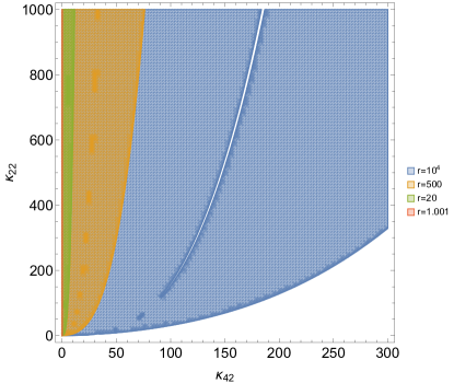
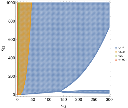
Figure 1: The phase space of $(\kappa_{42},\kappa_{22})$ for which the shadowed regions mean ${\hat{c}}_{r}^{2}\geq 0$, i.e., the radial Laplacian condition gets satisfied. The blue, orange, green and red shadowed regions correspond to $r=10^{4},\;500,\;20,\;1.001$ respectively. Upper panel: $\mathfrak{k}=1$; lower panel: $\mathfrak{k}=-1$. Here we have set $l=2$. Notice that, in here only the first quadrant of $(\kappa_{42},\kappa_{22})$ are considered since $\kappa_{42}$ and $\kappa_{22}$ are defined to be positive (cf., Sec.III).

To monitor the behavior of ${\hat{c}}_{r}^{2}$ as a function of $r$, we plot it out in the phase space of $(\kappa_{42},\kappa_{22})$ by setting $l=2$ in Fig. 1 for various $r$’s, in which both $\mathfrak{k}=\pm 1$ cases are considered. At those colorful shadowed regions the radial Laplacian condition, viz., ${\hat{c}}_{r}^{2}\geq 0$, gets satisfied. In there the quantity ${\hat{c}}_{r}^{2}$ is considered at different positions by varying $r$. We observe from Fig. 1 that the ”stable region” is shrinking as $r$ approaching the event horizon $r=1$. What is omitted in Fig. 1 is that the stable region will disappear if $r$ is sufficiently close to $1$, e.g., when $r=1+10^{-20}$. That means we definitely have this kind of instability no matter how the cupling parameters are chosen.

To make it more manifest, let us consider the quantity ${\hat{c}}_{r}^{2}$ in the neighborhood of event horizon $r=1$ (without setting $l$ to a specific value) and insert the full expressions supplemental1 . That leads to

$$\left.{\hat{c}}_{r}^{2}\right|_{r\to 1} = -\frac{2}{81}(r-1)^{2}\left(16\sqrt{6}\pi\kappa_{42}\sqrt{\frac{\kappa_{42}}{\kappa_{22}}}\mathfrak{k}-9\right)^{2}$$ (3.2)

$$+{\cal O}(r-1)^{3}.$$

Thus, for any combination of the coupling parameters, the radial Laplacian instability always exists in the neighborhood of $r=1$, as we mentioned above. Such a result is actually consistent with the conclusions given in Minamitsuji2022 ; Kobayashi2012 ; Kobayashi2014 .

IV Conclusions

In this paper we focus on a specific subclass of Horndeski theory describing by the action (2.1). Thank to a set of analytic background solutions (II) (with their deviations from that of GR are mainly characterized by two coupling parameters), we are able to systematically investigate the odd-parity gravitational perturbation to that background and extract the 2nd-order Lagrangian of the theory. With suitable mathematical techniques, the original Lagrangian finally reduced to the form of (2.3), with just one degree of freedom as expected. On top of that, we further run the stability analysis (see., e.g., Tsujikawa21 ; Kase2023 ; Kase2018 ) and demonstrate how the instability emerges.

First of all, certain constraints to the coupling parameters are identified from the no-ghost condition [cf., (III)]. Based on that, the following calculations can be simplified. This enables us to calculate and analyze the radial Laplacian stability condition within the valid phase space of (reduced) coupling parameters (cf., Fig.1). In Fig.1 we learn that such a stability condition requires additional constraints to the coupling parameters. More importantly, this stability condition tends to be broken in the neighborhood of event horizon $r=1$. Indeed, by using the asymptotic expansion of the criterion ${\hat{c}}_{r}^{2}$ [cf., (3.2)], it is clear that this condition will not be preserved anymore as $r\to 1$ [although we also notice that such a condition can be satisfied right at the point $r=1$, since we precisely have ${\hat{c}}_{r}^{2}(r=1)=0$] no matter how the coupling parameters are chosen. We thus conclude that the set of background solutions (II) are not stable and needs to be excluded from the valid solutions, which is consistent with the predictions given in Minamitsuji2022 .

Notice that, setting those coupling parameters to zero (as in the GR limit) in the final criterion or discriminant [cf., (3.2)] will not always simply bring us back to that of GR, different from what we have seen at the Lagrangian level. In Tsujikawa21 ; Kobayashi2014 we also observed similar phenomena. This implies that (in)stability of a theory could be a comprehensive effect and it is not necessary for the criterion to behave like a perturbation to the stable GR case. It is also interesting to mention that, as we see from the Fig.1, the most stringent constraint to the coupling parameters are given by the analysis within the neighborhood of $r=1$ (instead of the other positions that far from the event horizon). That is similar to the situation shown in Kase2018 .

In the future, we can move to other background solutions and models of the Horndeski theory. By referring Minamitsuji2022 , we can pay more attention to those stable cases. In principle, the corresponding stability analysis can not only help us bring constraints to the model but also give a reduced Lagrangian as a byproduct, which can serve for the QNM calculations in the next step. With more models investigated, it is also possible to extract some common features by using the conclusions from different cases.

References

- (1) B.P. Abbott, et al., [LIGO/Virgo Scientific Collaborations], Observation of Gravitational Waves from a Binary Black Hole Merger, Phys. Rev. Lett. 116, 061102 (2016).
- (2) A. Einstein, Näherungsweise Integration der Feldgleichungen der Gravitation, Sitzungsber. K. Preuss. Akad. Wiss. 1, 688-696 (1916).
- (3) B.P. Abbott, et al., [LIGO/Virgo Collaborations], GWTC-1: A Gravitational-Wave Transient Catalog of Compact Binary Mergers Observed by LIGO and Virgo during the First and Second Observing Runs, Phys. Rev. X9, 031040 (2019).
- (4) B.P. Abbott, et al., [LIGO/Virgo Collaborations], Open data from the first and second observing runs of Advanced LIGO and Advanced Virgo, SoftwareX, Volume 13, 100658 (2021).
- (5) B.P. Abbott, et al., [LIGO/Virgo Collaborations], GW190425: Observation of a Compact Binary Coalescence with Total Mass , ApJL 892 L3 (2020); https://www.ligo.caltech.edu.
- (6) B.P. Abbott, et al., [LIGO/Virgo/KAGRA Collaborations], GWTC-3: Compact Binary Coalescences Observed by LIGO and Virgo During the Second Part of the Third Observing Run, arXiv:2111.03606v1 [gr-qc].
- (7) C. J. Moore, R. H. Cole and C. P. L. Berry, Gravitational-wave sensitivity curves, Class. Quantum. Grav. 32, 015014 (2015).
- (8) Y. Gong, J. Luo and B. Wang, “Concepts and status of Chinese space gravitational wave detection projects,” Nature Astron. 5, no.9, 881-889 (2021).
- (9) https://cosmicexplorer.org.
- (10) ET Steering Committee Editorial Team, ET design report update 2020, ET-0007A- 20 (2020); https://www.et-gw.eu/.
- (11) https://www.lisamission.org.
- (12) S. Liu, Y. Hu, et al., Science with the TianQin observatory: Preliminary results on stellar-mass binary black holes, Phys. Rev. D101, 103027 (2020).
- (13) C.-F. Shi, et al., Science with the TianQin observatory: Preliminary results on testing the no-hair theorem with ringdown signals, Phys. Rev. D100, 044036 (2019).
- (14) W.-H. Ruan, Z.-K. Guo, R.-G. Cai, Y.-Z. Zhang, Taiji Program: Gravitational-Wave Sources, Int. J. Mod. Phys. A 35, No. 17, 2050075 (2020).
- (15) S. Kawamura, et al., Current status of space gravitational wave antenna DECIGO and B-DECIGO, arXiv:2006.13545.
- (16) C. Zhang, A. Wang and T. Zhu, Odd-parity perturbations of the wormhole-like geometries and quasi-normal modes in Einstein-Æther theory, JCAP 05 (2023) 059.
- (17) C. Zhang, Y. Gong, D. Liangc and B. Wang, Gravitational waves from eccentric extreme mass-ratio inspirals as probes of scalar fields, JCAP 06 (2023) 054.
- (18) E. Berti, K. Yagi, H. Yang, N. Yunes, Extreme gravity tests with gravitational waves from compact binary coalescences: (II) ringdown, Gen. Relativ. Grav. 50, 49 (2018).
- (19) S. Chandrasekhar, the mathematical theory of black holes, Oxford classic texts in the physical sciences (Oxford Press, Oxford, 1992).
- (20) S. Iyer, Black-hole normal modes: A WKB approach. II. Schwarzschild black holes, Phys. Rev. D35, 3632 (1987).
- (21) Zack Carson and Kent Yagi, Probing Einstein-dilaton Gauss-Bonnet gravity with the inspiral and ringdown of gravitational waves, Phys. Rev. D101, 104030 (2020).
- (22) E. Berti, V. Cardoso and A. O. Starinets, Quasinormal modes of black holes and black branes, Class. Quantum. Grav. 26, 163001 (2009).
- (23) W. Liu, X. Fang, J. Jing, et al., Gauge invariant perturbations of general spherically symmetric spacetimes, Sci. China Phys. Mech. Astron. 66, 210411 (2023).
- (24) C. Zhang, T. Zhu and A. Wang, Gravitational axial perturbations of Schwarzschild-like black holes in dark matter halos, Phys. Rev. D104, 124082 (2021).
- (25) R. Kase and S. Tsujikawa, Black hole perturbations in Maxwell-Horndeski theories, Phys. Rev. D107, 104045 (2023).
- (26) R. Gannouji and Y.R. Baez, Stability of generalized Einstein-Maxwell-scalar black holes, J. High Energ. Phys. 02, 020 (2022).
- (27) S. Tsujikawa, C. Zhang, X. Zhao and A. Wang, Odd-parity stability of black holes in Einstein-Aether gravity, Phys. Rev. D104, 064024 (2021).
- (28) Keitaro Tomikawa and Tsutomu Kobayashi, Perturbations and quasinormal modes of black holes with time-dependent scalar hair in shift-symmetric scalar-tensor theories, Phys. Rev. D104, 064024 (2021).
- (29) Masato Minamitsuji and Kei-ichi Maeda, Black hole thermodynamics in Horndeski theories, Phys. Rev. D108, 084061 (2023).
- (30) S. Mironov and V. Volkova, In hot pursuit of a stable wormhole in beyond Horndeski theory, Phys. Rev. D107, 104061 (2023).
- (31) Yurika Higashino and Shinji Tsujikawa, Inspiral gravitational waveforms from compact binary systems in Horndeski gravity, Phys. Rev. D107, 044003 (2023).
- (32) Hou-Yu Lin and Xue-Mei Deng, Dynamics of test particles around hairy black holes in Horndeski’s theory, Annals of Physics 455 (2023) 169360.
- (33) Tsutomu Kobayashi, Hayato Motohashi, and Teruaki Suyama, Black hole perturbation in the most general scalar-tensor theory with second-order field equations: The odd-parity sector, Phys. Rev. D85, 084025 (2012).
- (34) M Minamitsuji, K. Takahashi and S. Tsujikawa, Linear stability of black holes with static scalar hair in full Horndeski theories: Generic instabilities and surviving models, Phys. Rev. D106, 044003 (2022).
- (35) T. Kobayashi, H. Motohashi and T. Suyama, Black hole perturbation in the most general scalar-tensor theory with second-order field equations. II. The even-parity sector, Phys. Rev. D89, 084042 (2014).
- (36) E. Babichev, C. Charmousis, G. Esposito-Farèse and A. Lehébel, Hamiltonian unboundedness vs stability with an application to Horndeski theory, Phys. Rev. D98, 104050 (2018).
- (37) Tsutomu Kobayashi, Horndeski theory and beyond: a review, Rep. Prog. Phys. 82 086901 (2019).
- (38) S. E. P. Bergliaffa, R. Maier, and N. d. O. Silvano (2021), arXiv:2107.07839.
- (39) M.Maggiore, Gravitational Waves, Volume 2: Astrophysics and Cosmology (Oxford University Press, Oxford, UK, 2018).
- (40) F.J.Zerilli, Gravitational Field of a Particle Falling in a Schwarzschild Geometry Analyzed in Tensor Harmonics, Phys. Rev. D2, 10 (1970).
- (41) J. E. Thompson, H. Chen and B. F. Whiting, Gauge invariant perturbations of the Schwarzschild spacetime, Class. Quantum Grav. 34 174001 (2017).
- (42) L. Heisenberg, R. Kase and S. Tsujikawa, Odd-parity stability of hairy black holes in U(1) gauge-invariant scalar-vector-tensor theories, Phys. Rev. D97, 124043 (2018).
- (43) A. Ganguly, R. Gannouji, M. Gonzalez-Espinoza and C. Pizarro-Moya, Black hole stability under odd-parity perturbations in Horndeski gravity, Class. Quantum Grav. 35 (2018) 145008 (18pp).
- (44) T. Regge and J. A. Wheeler, Stability of a Schwarzschild Singularity, Phys. Rev. 108, 4 (1957).
- (45) G. B. Arfken, H. J. Weber and F. E. Harris Mathematical Methods for Physicists (7th ed) (Elsevier Inc, UK, 2013).
- (46) J. R. Taylor, Classical mechanics (University Science Books, USA, 2005).
- (47) https://github.com/bjsheep/supplemental20240104.git.