SparseDM: Toward Sparse Efficient Diffusion Models

Abstract

Diffusion models have been extensively used in data generation tasks and are recognized as one of the best generative models. However, their time-consuming deployment, long inference time, and requirements on large memory limit their application on mobile devices. In this paper, we propose a method based on the improved Straight-Through Estimator to improve the deployment efficiency of diffusion models. Specifically, we add sparse masks to the Convolution and Linear layers in a pre-trained diffusion model, then use design progressive sparsity for model training in the fine-tuning stage, and switch the inference mask on and off, which supports a flexible choice of sparsity during inference according to the FID and MACs requirements. Experiments on four datasets conducted on a state-of-the-art Transformer-based diffusion model demonstrate that our method reduces MACs by $50\%$ while increasing FID by only 1.5 on average. Under other MACs conditions, the FID is also lower than 1$\sim$137 compared to other methods.

1 Introduction

Diffusion Models (DM) (Song et al., 2021; Karras et al., 2022) have been one of the core generative modules in various computer vision tasks with their advantages on both sample quality and mode coverage. Generally, they are composed of two stages : a forward/diffusion process that perturbs the data distribution to learn the time-dependent score functions, and a reverse/sampling process that generates data samples from a prior distribution in an iterative manner. However, their slow inference speed and heavy computational load during inference process inevitably restrict their applications on most mobile devices.

To reduce the computational load in the inference process of diffusion models, various methods have been proposed to minimize the number of inference steps, such as the training-free samplers (Bao et al., 2022; Zhao et al., 2023; Lu et al., 2022, 2023; Zheng et al., 2023; Chen et al., 2023) and the distillation methods (Salimans & Ho, 2022; Luo et al., 2023b, a). However, their sample quality is still unsatisfactory as a few sampling steps cannot faithfully reconstruct the high-dimensional data space, e.g., the image or video samples. This problem is even more pronounced on mobile devices with limited computing capabilities. Simultaneously, a few works explore reducing the Multiple-Accumulate operations (MACs) at each inference step (Bolya & Hoffman, 2023; Fang et al., 2023b). However, their work cannot be accelerated on GPUs. Since DM is an intensive model parameter calculation, NVIDIA Ampere architecture GPU supports a 2:4 sparse (4-weights contain 2 non-zero values) model calculation, which can achieve nearly 2 times calculation acceleration (Pool & Yu, 2021; Mishra et al., 2021). Although structural pruning (Fang et al., 2023b) and sparse models (Frantar & Alistarh, 2023) have been used in DM, 2:4 structured sparsity or dynamic multi-scale sparse inference has not been implemented. Our method aims to reduce MACs at each step through 2:4 and multi-scale sparsity.

Recently, several popular computational architectures, such as NVIDIA Ampere architecture and Hopper GPUs, have developed acceleration methods for model inference and have been equipped with fine-grained structured sparse capabilities. A common requirement of these acceleration techniques is the 2:4 sparse mode which only preserves 2 of the 4 adjacent weights of a pre-trained model, i.e., requires a sparsity rate of $50\%$. Given this sparsity, the acceleration techniques only process the non-zero values in matrix multiplications, theoretically achieving a 2x speedup. In essence, a diffusion model supporting the 2:4 sparsity mode can reduce $50\%$ computational load at each inference step, which is valuable when considering the iterative refinement process in generation. To the best of our knowledge, previous works have not explored maintaining the sample quality of diffusion models with a 2:4 or other flexible sparsity mode, which motivates us to present the techniques in this work.

We use a state-of-the-art Transformer-based DM, named U-ViT (Bao et al., 2023), to analyze the shortcomings of existing 2:4 structured sparse tools. Also, we manually design a half-size DM network to test FID and MACs. From Table 1, we can see that simply reducing the U-ViT model parameters by nearly $50\%$ may cause FID to collapse catastrophically. Automatic Sparsity (ASP) (Pool & Yu, 2021; Mishra et al., 2021)) for model sparse training consumes a lot of GPU time, but FID is poor. Therefore, for DM, we need to redesign the pruning method to reduce the amount of calculation and maintain FID as much as possible.

Table 1: The results of manually redesigning the UViT model and sparse pruning the UViT model using ASP. UViT Small is from the U-ViT method. Half UViT Small is set to half the depth and number of heads of UViT Small. ASP is the method of sparse pruning from Nvidia.

Datasets Models Methods FID MACs (G) CIFAR10 32x32 UViT Small U-ViT 3.20 11.34 Half UViT Small U-ViT 678.20 5.83 UViT Small ASP 319.87 5.76 CelebA 64x64 UViT Small U-ViT 2.87 11.34 Half UViT Small U-ViT 441.37 5.83 UViT Small ASP 438.31 5.76

This paper proposes a new method for simultaneously implementing 2:4 structured sparsity and dynamic multi-scale sparse inference. (1) Sparse masks are applied to the Convolution and Linear layers; (2) we use progressive sparsity to train the model and provide an interpretation; (3) we use switchable masks on the inference according to Frechet Inception Distance (FID) (Heusel et al., 2017) and MACs requirement.

Our contributions can be listed as follows:

• We propose a method that simultaneously achieves 2:4 structured sparse inference and multi-scale dynamic sparse pruning for DM.

• To the best of our knowledge, we are the first to study progressive sparse finetuning to get a better sparsity DM with a Transformer backbone and provide an explanation.

• We conduct experiments on four datasets. The average FID of 2:4 sparse (2x speedup) DM is only increased by 1.5 compared with the dense model. Our trained 2:4 sparse model performs better inference results than all existing methods.

• Testing nine scales, with similar MACs for each scale, our multi-scale dynamic sparse inference FID is $1\sim 137$ lower than other methods.

2 Problem Formulation

Diffusion Models The diffusion model is divided into a forward process and a backward process. The forward process is a step-by-step process of adding noise to the original image to generate a noisy image, generally formalized as a Markov chain process. The reverse process is to remove noise from a noisy image and restore the original image as much as possible. Gaussian mode was adopted to approximate the ground truth reverse transition of the Markov chain. The training process of diffusion models is the process of establishing noise prediction models. The loss function of DM is minimizing a noise prediction objective. The forward process is formalized as:

$$q({\bm{x}}_{1:T}|{\bm{x}}_{0})=\prod_{t=1}^{T}q({\bm{x}}_{t}|{\bm{x}}_{t-1}),$$ (1)

where ${\bm{x}}_{t}$ is input data at $t$. The backward process is formalized as:

$${\bm{\mu}}_{t}^{*}({\bm{x}}_{t})=\frac{1}{\sqrt{\alpha_{t}}}\left({\bm{x}}_{t}-\frac{\beta_{t}}{\sqrt{1-\overline{\alpha}_{t}}}\mathbb{E}[{\bm{\epsilon}}|{\bm{x}}_{t}]\right),$$ (2)

where $\alpha_{t}$ and $\beta_{t}$ are the noise schedule at $t$, $\alpha_{t}+\beta_{t}=1$. $\overline{\alpha}_{t}=\prod_{i=1}^{t}\alpha_{i}$, and ${\bm{\epsilon}}$ is the standard Gaussian noises added to ${\bm{x}}_{t}$. The DM training is a task of minimizing the noisy prediction errors, expressed as:

$$\min_{\mathcal{W}}\mathcal{L}(\mathcal{W};\mathcal{D}),$$ (3)

where $\mathcal{D}$ is dataset, $\mathcal{L}$ is loss function, $\mathcal{W}$ is dense weights. The DM inference, data generation, is expressed as:

$${\bm{y}}_{t}=\mathcal{F}(\mathcal{W};{\bm{x}}_{t}).$$ (4)

where $\mathcal{F}$ is trained DM, ${\bm{y}}_{t}$ is the output of DM inference.

Sparse Pruning Sparse network computation is an effective method to reduce MACs in deep networks and accelerate computation. Currently, one-shot sparse training and progressive sparse training are commonly used.

The one-shot training method is easy to use, and the steps are as follows (Mishra et al., 2021; Pool & Yu, 2021): Train a regular dense model. Prune the weights on the fully connected and convolutional layers in a 2:4 sparse mode. Retrain the pruned model. The one-shot pruning is expressed as:

$$\begin{split}\widetilde{\mathcal{W}}&=\mathcal{W}\odot\mathcal{M},\end{split}$$ (5)

where, $\widetilde{\mathcal{W}}$ is the sparse weight after the dense weight $\mathcal{W}$ is pruned, recorded as $\widetilde{\mathcal{W}}\leftarrow\text{Pruning}(\mathcal{W})$, $\mathcal{M}$ is a 0-1 mask, $\mathcal{M}$ is the ($N$:$M$) sparse mask ($M$-weights contain $N$ non-zero values), $\odot$ represents element-wise multiplication.

One-shot sparse pruning can cover most tasks and achieve speedup without losing accuracy. However, for some difficult tasks that are sensitive to changes in weight values, doing sparse training for all weights at once will result in a large amount of information loss (Han et al., 2015). With the same number of tuning iterations, progressive sparse training can achieve higher model accuracy than one-shot sparse training. Assume that the sparsity rate corresponding to $\mathcal{M}_{0}$ mask is $N_{0}:M_{0}=1:1$ ($\frac{1}{1}=100\%$), that is, there is no sparsity for $N:M$ sparse matrices. Suppose there are $k$ masks $[\mathcal{M}_{1},\mathcal{M}_{2},...,\mathcal{M}_{k}]$, and the sparsity rate corresponding to each mask is less than $100\%$. The progressive sparse process is formalized as:

$$\widetilde{\mathcal{W}}=\mathcal{W}\odot\mathcal{M}_{i},~{}~{}\mathcal{M}_{i}\in[\mathcal{M}_{1},\mathcal{M}_{2},...,\mathcal{M}_{k}].$$ (6)

3 Sparse Finetuning DM

In this section, we introduce our proposed framework in detail. We start with the overall framework of our proposal. Then, we present the finetuning DM with sparse masks for reducing MACs and prepare for 2:4 sparse GPU acceleration. Moreover, we introduce the training and inference with multi-scale sparse masks for enhancing the DM. Fig. 1 shows an overview of the proposed framework.

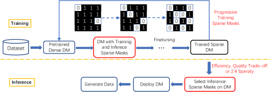
Figure 1: Framework Overview. Training is the process of training with a progress sparse mask. The inference is to dynamically adjust the mask switch according to the needs of the deployment environment to achieve a trade-off of efficiency and quality.

3.1 Straight-Through Estimator for Sparse Training

A straightforward solution for training an $N$:$M$ sparsity network is to extend the Straight-through Estimator (STE) (Bengio et al., 2013) to perform online magnitude-based pruning and sparse parameter updating. The concrete formula is described as:

$$\mathcal{W}_{t+1}\leftarrow\mathcal{W}_{t}-\gamma_{t}g(\widetilde{\mathcal{W}^{(N:M)}_{t}})$$ (7)

where $\gamma$ is learning rate, $g$ is gradient. In STE, a dense network is maintained during the training process. In the forward pass, the dense weights $\mathcal{W}$ are projected into sparse weights $\widetilde{\mathcal{W}^{(N:M)}}=S(\mathcal{W},N,M)$ satisfying $N$:$M$ sparsity. $S(\cdot)$ is projection function. The sparse DM training task is expressed as:

$$\min_{S(\mathcal{W},N,M)}\mathcal{L}(\mathcal{W};\mathcal{D})$$ (8)

The sparse DM inference is expressed as:

$${\bm{y}}_{t}=\mathcal{F}(\widetilde{\mathcal{W}^{(N:M)}};{\bm{x}}_{t})$$ (9)

To mitigate the negative impact of the approximate gradient calculated by vanilla STE, Sparse Fine Straight-through Estimator (SR-STE) (Zhou et al., 2021) incorporates sparse mask information into the backward propagation process. The right part of the update formula is modified as :

$$\mathcal{W}_{t}-\gamma_{t}\left(g(\widetilde{\mathcal{W}^{(N:M)}_{t}})+\lambda_{W}(\mathcal{W}_{t}-\widetilde{\mathcal{W}^{(N:M)}_{t}})\right)$$ (10)

However, the existing STE methods use fixed sparsity rates for model training. We must retrain the model each time to obtain inference models with different sparsity rates, which is unacceptable for training expensive DM models. To obtain extremely sparse DM, jumping directly from the dense model to the extremely sparse model, such as 1:32 ($\frac{1}{32}=0.03125$) sparsity, for training and using the extremely sparse weight gradient for reverse propagation can easily lead to the collapse of the trained model.

3.2 Progressive Sparse Finetuning Diffusion Model

To achieve better high-sparsity DM, we add multi-scale masks for progressive training of DM, thereby improving the sparse training method based on STE.

To achieve 2:4 sparse GPU acceleration, the current sparse training method is to directly train from a dense model with a sparsity rate of 0 to a sparse model with a sparsity rate of $50\%$, which can easily cause information loss. Due to the lengthy training process aimed at obtaining $50\%$ of the sparse model, we adopt a progressive sparse training process, ensuring we can obtain $50\%$ of the sparse model with minimal information loss. We add progressive sparse masks to existing STE-based methods. The progressive sparse DM training task is expressed as :

$$\min_{S(\mathcal{W}\odot\mathcal{M})}\mathcal{L}(\mathcal{W};\mathcal{D};[\mathcal{M}_{1},\mathcal{M}_{2},...,\mathcal{M}_{k}]),$$ (11)

The projection function $S(\cdot)$, which is non-differentiable during back-propagation, generates the $N$:$M$ sparse sub-network on the fly. To get gradients during back-propagation, STE computes the gradients of the sub-network $g(\widetilde{\mathcal{W}})=\bigtriangledown_{\widetilde{\mathcal{W}}}\mathcal{L}(\widetilde{\mathcal{W}};\mathcal{D})$ based on the sparse sub-network $\widetilde{\mathcal{W}}$, which can be directly back-projected to the dense network as the approximated gradients of the dense parameters. The approximated parameter update rule for the dense network can be formulated as:

$$\begin{split}\mathcal{W}_{t+1}&\leftarrow\mathcal{W}_{t}-\gamma_{t}g(\widetilde{\mathcal{W}^{(N_{i}:M_{i})}_{t}}),~{}~{}i\in[1,k]\end{split}$$ (12)

And we need to specify that for every $i$, $N_{i}$ and $M_{i}$ are applied in a selected time interval $[s_{i},t_{i}]$. And this STE-based method could be easily modified to SR-STE-based. The right part should be Equ. (13) with $i\in[1,k]$.

$$\begin{split}\mathcal{W}_{t}-\gamma_{t}\left(g(\widetilde{\mathcal{W}^{(N_{i}:M_{i})}_{t}})+\lambda_{W}(\mathcal{W}_{t}-\widetilde{\mathcal{W}^{(N_{i}:M_{i})}_{t}}))\right)\end{split}$$ (13)

The sparse finetuning diffusion model is implemented in Algorithm 1. We designed a pruning method based on computational constraints to obtain faster models from a stable large network model. Under the constraint of computational complexity, we can obtain the DM with the minimum FID loss. Conv and Linear in the network structure are both potential sparse objects. We set different masks at each layer of the network structure, which makes it easier to switch masks at each layer flexibly. To achieve acceleration on NVIDIA GPU, this article temporarily does not consider sparse pruning that exceeds 50% (2:4 Sparsity) of the entire large model. Searching for DM with better FID is also possible in the above optimization process. As a result, we have achieved layer-wise sparse pruning under the guidance of FID improvement targets. It can also be achieved if it is necessary to replace the DM evaluating target, such as Structural Similarity (SSIM) (Wang et al., 2004).

Algorithm 1 Sparse Finetuning Diffusion Model

Input: $\mathcal{B}$ is the bound of MACs, such as 2:4 sparsity ($50\%$ sparsity). $[\mathcal{M}_{1},\mathcal{M}_{2},...,\mathcal{M}_{k}]$ is $k$ sparse masks.
Output: Minimize FID loss of DM under given MACs constraints.

1:  /*Searching mask change interval*/

2:  Train DM with the normal process by Equ. (3)

3:  Generate data and Calc. it’s $fid_{0}$ by Equ. (4) and (16)

4:  while Select mask $\mathcal{M}_{i}\in[\mathcal{M}_{1},\mathcal{M}_{2},...,\mathcal{M}_{k}]$ do

5:     Add the sparse mask $\mathcal{M}_{i}$ for each layer

6:     Finetune DM with the mask by Equ. (8) and (7)

7:     Generate data via DM with mask by Equ. (9)

8:     Get the data $fid_{i}$ corresponding to each mask

9:     Calculate FID loss with $fid_{i}-fid_{0}$ by Equ. (16)

10:  end while

11:  Select the best mask interval for FID under bound $\mathcal{B}$

12:  /*Progressive Finetuning DM with sparse masks*/

13:  Set DM to the least sparse mask and fine-tune

14:  while Select the next level mask from the interval do

15:     Finetune DM with the mask by Equ. (11) and (13)

16:  end while

17:  Progressive trained DM with minimizing FID loss

18:  return Minimize FID loss of DM under bound $\mathcal{B}$

3.3 Interpretability Analysis

This subsection analyzes and interprets the effectiveness of progressive STE-based sparse training for DM. We believe progressive sparse optimization is easier starting from the dense model than direct highly sparse optimization. Below, we would like to explain the intuition behind our approach in detail.

Firstly, we consider the difficulty that comes from exiting STE-based methods. STE-based methods indicate that updating dense weights with approximate gradients increases optimization difficulty. Because imprecise gradients increase the probability that the optimizer will get stuck or lose, the optimizer often gets stuck in local minima. We therefore formalize the optimization problem for dense weights as a smooth function $f(x)$, and the optimization problem for 2:4-sparsity or high-sparsity weights as a steep function $g(x)$. As shown in Fig. LABEL:fig:opt1, an intuitive diagram of the shape of the $f(x)$ and $g(x)$ functions is given.

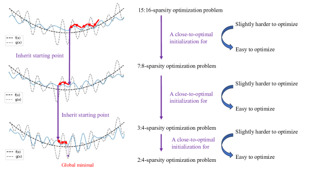
Figure 3: Progressive sparse training method intuition.

Due to the optimization difficulty mentioned above, it is difficult to train the optimal high-sparsity model using STE-based methods directly. Using our progressive masks makes optimization less difficult. A steep function is decomposed into multiple smoother functions through multiple intermediate sparsity masks, which is more conducive to the optimizer reaching the optimal point. We demonstrate this process in Fig. 3. The direction of the down arrows in the figure shows that the optimization difficulty of each child stage does not change much, but each progressive stage is more difficult to optimize than the initial stage since the starting points are expected to lie in the region closed to global optimal. From an intuitive perspective, the previous stage will end with a more optimized point. Each step is an easy optimization process. Compared with STE-based methods, the gradual optimization method can get better optimization results for $g(x)$.

3.4 Sparse Mask for Inference

According to different hardware, during the inference process, we implemented two schemes. The first category is an inference design for 2:4 sparse hardware acceleration. To achieve the best performance at a specific sparse rate, the 2:4 sparse mask is trained with progressive sparsity. The second category is dynamic mask design for MACs and FID trade-offs. To flexibly and dynamically adapt to different scenarios, such as calculation-efficient or resource-efficient, the model is only trained once, then dynamically planned layer-wise according to different scenarios, and then the mask is selected.

In diffusion model application, there will be different hardware computing capabilities, time requirements, and image production quality requirements. We need to control the amount of inference calculations dynamically. If there is no specified sparsity rate for the training process, we default to training at a 1:1 sparsity rate, which means only $\mathcal{M}_{0}$ masks are added during the training process. Then, during the inference process, dynamically adjust the sparsity rate layer-wise. ${\bm{y}}^{l}_{t}=\mathcal{F}(\widetilde{\mathcal{W}^{l}};{\bm{x}}_{t}),~{}l\in(0,L]$ is the $l$-th layer inference result. ${\bm{y}}^{l(N:M)}_{t}=\mathcal{F}(\widetilde{\mathcal{W}^{l(N:M)}};{\bm{x}}_{t}),~{}l\in(0,L]$ is the $l$-th layer with $N$:$M$ mask inference result. The formula for layer-wise different mask inference results is as:

$$\begin{split}{\bm{y}}^{l(N_{i}:M_{i})}_{t}=\mathcal{F}(\widetilde{\mathcal{W}^{l(N_{i}:M_{i})}};{\bm{x}}_{t}),~{}l\in(0,L]\end{split}$$ (14)

where $i\in[1,k]$.

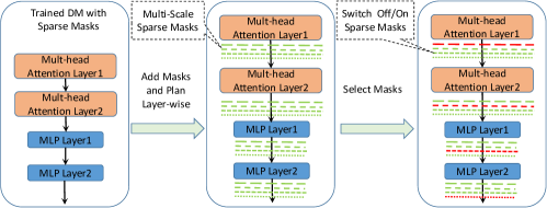
Figure 4: Inference process based on multiple sparsity rate masks. We add multi-scale masks to the diffusion model for each layer. We select masks off or on for each layer based on the overall sparsity ratio.

To more specifically select which layers have the mask on and which layers have the mask off, we classify the layers according to the position and function of each layer in the network. We divide U-ViT models into four major categories. The first type is nn.Conv, and nn.Conv is at the front end and the back end of the network. The second category is the nn.Linear layer of Attention. The third category of layers is nn.Linear in MLP. The fourth category is the embedding layer. This classification method avoids time-consuming evaluation of the effectiveness of each layer and improves planning efficiency for various mobile devices.

For the 2:4 sparse acceleration GPU, the structured sparsity function is mainly used in fully connected layers and convolutional layers that can provide 2:4 sparse weights. If the weights of these layers are pruned in advance, these layers can be accelerated using structured sparsity functions on GPU. 2:4 sparsity layer-wise inference is expressed as:

$${\bm{y}}^{l(2:4)}_{t}=\mathcal{F}(\widetilde{\mathcal{W}^{l(2:4)}};{\bm{x}}_{t}),~{}~{}l\in(0,L].$$ (15)

Through the above two layer-wise inference methods, flexible acceleration can be achieved on both hardware of 2:4 sparse acceleration GPU and various mobile devices.

4 Results and Discussion

In this section, we will compare and discuss the 2:4 sparsity rate optimization results and the efficiency, quality trade-off dynamic sparsity rate results

4.1 Experimental Settings

Evaluation Metrics In this paper, we concentrate primarily on two types of metrics: The efficiency metric is MACs; The quality metric is FID, which Equ. (16) calculates.

$$FID_{(x,g)}=\|\mu_{x}-\mu_{g}\|^{2}_{2}+T_{r}(\sigma_{x}+\sigma_{g}-2(\sigma_{x}\sigma_{g})^{0.5}).$$ (16)

where $T_{r}$ represents the trace of the matrix. $x$ and $g$ represent real pictures and generated pictures, $\mu$ represents the mean, and $\sigma$ is the covariance matrix. We generated 50,000 images and calculated FID together with the original images.

Baseline Methods We compare the performance of our method with the following baseline algorithm at 2:4 or multi-scale sparsity. Diff-Pruning (Fang et al., 2023b) is a method of structural pruning of diffusion models. ASP (Automatic SParsity) (Pool & Yu, 2021; Mishra et al., 2021) is a tool that enables 2:4 sparse training and inference for PyTorch models provided by Nvidia. Nvidia had developed a simple training workflow that can easily generate a 2:4 structured sparse network matching the accuracy of the dense network. To compare the performance of dynamic sparse mask, we give the results of inference with different sparsity rates. Finally, we provide the ablation study results of STE-based for the training process. We give the ablation study results of random and untrained masks for the inference process.

4.2 Result Comparison

2:4 Sparsity Results

Table 2: The comparison of 2: 4 ($50\%$ ) sparsity results. No Pruning is the method of U-ViT. U-ViT with LDM is U-ViT using Latent Diffusion Models (LDM) (Rombach et al., 2022) for data process. Diff-Pruning is a structural pruning method. ASP is the method of sparse pruning from NVIDIA.

Start DM Datasets Methods FID MACs (G) U-ViT CIFAR10 32x32 No Pruning 3.20 11.34 Diff-Pruning 12.63 5.32 ASP 319.87 5.76 Ours 4.23 5.67 CelebA 64x64 No Pruning 2.87 11.34 Diff-Pruning 11.35 5.32 ASP 438.31 5.76 Ours 3.52 5.67 U-ViT with LDM MS-COCO 256x256 No Pruning 5.95 11.34 Diff-Pruning 15.20 5.43 ASP 350.87 5.79 Ours 8.20 5.68 MS-COCO 256x256 (Deep) No Pruning 5.48 14.72 Diff-Pruning 16.92 7.12 ASP 340.69 7.43 Ours 6.84 7.37 ImageNet 256x256 No Pruning 3.40 76.66 Diff-Pruning 14.28 34.06 ASP 367.41 37.93 Ours 5.69 36.84

We experiment on four datasets (CIFAR10, CelebA, MS COCO 2014, and ImageNet) and four resolutions (32$\times$32, 64$\times$64, and 256$\times$256). We reduced the computational load by approximately $50\%$, and the FID only increased by 0.65$\sim$2.29 (1.51 on average). Especially for models of similar sizes, the higher the resolution, the better the FID effect, such as U-ViT on CIFAR10 32$\times$32 and CelebA 64$\times$64. This way, our method is more suitable for model acceleration in high-resolution and high-fidelity image generation.

In addition to changes in FID, it is also important to intuitively evaluate the data generated by the sparse acceleration model. From the generated images in Fig. LABEL:fig:samples, it can be seen that there is almost no difference between the images generated by our accelerated model and the images generated by the original model due to a slight change in FID.

Dynamic Sparsity Results Except for the $50\%$ sparsity ratio of 2:4, we have also conducted experiments on other sparsity ratios. Since the ASP method is a sparsity tool provided by Nvidia for GPU hardware acceleration, no other sparsity ratios are provided. The following is mainly a comparison of different sparsity levels with other methods.

Fig. LABEL:fig:sparse_inference(a) shows the effect of different sparsity ratios on FID. We evaluated ten sparsity ratios with 32:32, 31:32, 15:16, 7:8, 3:4, 2:4, 1:4, 1:8, 1:16, and 1:32. As shown in this figure, it does not mean that the greater the sparsity, the better the FID. For example, the sparsity of 31:32 ($\frac{31}{32}=0.96875$) and the sparsity of 15:16 ($\frac{15}{16}=0.9375$), which is higher than the FID of 7:8 with a sparsity of ($\frac{7}{8}=0.875$). In addition to GPU hardware acceleration, the sparsity ratio 2:4 also achieves good FID, proving the 2:4 sparse mask training and inference effectiveness. Based on the above observations, we choose the starting point of progressive sparseness to be a sparsity of 7:8. Fig. LABEL:fig:sparse_inference(b) shows that on the dataset CIFAR10, the FID performance of progressive sparse training is significantly better than that of fixed sparse training, especially for models with extremely low sparsity rates. Except for the 2:4 sparsity ratio, Fig. LABEL:fig:sparse_inference(c) shows that our method achieves significantly lower FID than the Diff-Pruning method at different sparse ratios on CIFAR10 and CelebA64.

4.3 Ablation Study

Our method is to perform sparse mask fine-tuning on the existing trained model. Masks need to be dynamically trained during the training process. To better demonstrate the rationality of our method design and the necessity of each step, we designed two ablation experiments. One is to fix the mask during the training process and not perform dynamic training. The other is the STE-based method.

STE Sparse Training As shown in Fig. LABEL:fig:sparse_inference(d) and LABEL:fig:sparse_inference(e), on datasets CIFAR10 and CelebA64, whether it is 2:4 sparse or multi-scale sparse, the training method of STE is worse than our method, mainly because our method adds progressive sparse training.

Sparse Mask Inference Unlike our trained masks, we generate untrained sparse masks for sparse pruning diffusion models. Based on the sparsity ratio, we randomly generate a random mask. As shown in Fig. LABEL:fig:sparse_inference(f), on datasets CIFAR10, the result of the random mask is the worst. The untrained mask is better than the random mask method but worse than ours because the mask did not participate in training. At the highest sparsity rate, our method achieves a FID 137 lower than that of random masks. At the lowest sparsity rate, our method achieves 1 less FID than the untrained mask.

5 Related Work

5.1 N: M Sparsity

A neural network with $N$:$M$ sparsity ($M$-weights contains $N$ non-zero values) satisfies that, in each group of $M$ consecutive weights of the network, there are at most $N$ weights have non-zero values (Zhou et al., 2021; Chmiel et al., 2022). APEX’s Automatic SParsity (ASP) (Pool & Yu, 2021; Mishra et al., 2021)) is a 2:4 sparse tool provided by NVIDIA. This tool obtains a 2:4 sparse network and can achieve nearly 2x runtime speedup on NVIDIA Ampere and Hopper architecture GPUs (Nvidia, 2020). A provable and efficient method for finding N: M transposed masks for accelerating sparse neural training (Hubara et al., 2021). Compared with dense networks, sparse network training has gradient changes, and methods such as STE (Bengio et al., 2013) should be used to improve training performance. In the forward stage, sparse weight is obtained by pruning dense weight. In the backward stage, the gradient w.r.t. sparse weight will be directly applied to dense weight. SR-STE (Zhang et al., 2022) keeps the forward pass consistent with STE and improves the backward pass. In the backward pass, the dense weights are updated not only by the derivatives of the sparse weights but also by the mask matrix of the pruned sparse weights. DominoSearch (Sun et al., 2021) found mixed N: M sparsity schemes from pre-trained dense, deep neural networks to achieve higher accuracy than the uniform-sparsity scheme with equivalent complexity constraints. The N: M sparse method is also used in SparseGPT (Frantar & Alistarh, 2023) to accelerate the LLM generation model GPT. Although many N: M sparse methods exist, none have been proven effective for sparse DM.

5.2 Diffusion Model Pruning

Pruning is one of the most used methods to reduce the calculation time of DNN, including DM. The pruning method was divided into structured pruning and unstructured pruning. Structural pruning aims to physically remove a group of parameters, thereby reducing the size of neural networks. In contrast, unstructured pruning involves zeroing out specific weights without altering the network structure (Fang et al., 2023a). Sparsity can reduce the memory footprint of DM to fit mobile devices and shorten training time for ever-growing networks (Hoefler et al., 2021). Pay attention to features and selection of useful features for the target dataset (Wang et al., 2020), which can also reduce computational complexity. The parameter-grouping patterns vary widely across different models, making architecture-specific pruners, which rely on manually designed grouping schemes, non-generalizable to new architectures. Depgraph (Fang et al., 2023a) can tackle general structural pruning of arbitrary architecture. Structured sparsity was also used for large language models (Ma et al., 2023; Frantar & Alistarh, 2023; Guo et al., 2023). Because Transformer has been proven to outperform the other networks in multiple applications, including DM. ToMe (Bolya & Hoffman, 2023) merge redundant tokens of Transformer. There are also proposals for early exiting for accelerated inference in DM (Moon et al., 2023). Although there are many pruning methods for DM, either the sparse model FID is poor or structured 2:4 sparsity is not implemented.

6 Conclusion

In this paper, we studied how to improve the efficiency of DM by sparse matrix for 2:4 sparse acceleration GPU and mobile devices. The existing STE-based methods make it difficult to optimize sparse DM. To address this issue, we propose a progressive approach to smooth the optimized surface gradually. To deploy the model on various computing devices, we adjust the MACs of model inference by setting different sparse rates on the sparse mask. Our method is tested on the latest Transformer-based DM, U-ViT. We trained the 2:4 and multi-scale sparse models to perform better than other methods. Our approach also provides an effective solution for DM deployment on NVIDIA Ampere architecture GPUs, with the expectation of achieving 2x acceleration.

7 Potential Broader Impacts

Our DM acceleration technology may be used for personal photo synthesis on mobile phones, such as facial synthesis. We need to consider and control these risks.

References

- Bao et al. (2022) Bao, F., Li, C., Zhu, J., and Zhang, B. Analytic-dpm: an analytic estimate of the optimal reverse variance in diffusion probabilistic models. In International Conference on Learning Representations, 2022.
- Bao et al. (2023) Bao, F., Nie, S., Xue, K., Cao, Y., Li, C., Su, H., and Zhu, J. All are worth words: A vit backbone for diffusion models. In Proceedings of the IEEE/CVF Conference on Computer Vision and Pattern Recognition, pp. 22669–22679, 2023.
- Bengio et al. (2013) Bengio, Y., Léonard, N., and Courville, A. Estimating or propagating gradients through stochastic neurons for conditional computation. arXiv preprint arXiv:1308.3432, 2013.
- Bolya & Hoffman (2023) Bolya, D. and Hoffman, J. Token merging for fast stable diffusion. In Proceedings of the IEEE/CVF Conference on Computer Vision and Pattern Recognition Workshop, pp. 4598–4602, 2023.
- Chen et al. (2023) Chen, Z., He, G., Zheng, K., Tan, X., and Zhu, J. Schrodinger bridges beat diffusion models on text-to-speech synthesis. arXiv preprint arXiv:2312.03491, 2023.
- Chmiel et al. (2022) Chmiel, B., Hubara, I., Banner, R., and Soudry, D. Optimal fine-grained n: M sparsity for activations and neural gradients. arXiv preprint arXiv:2203.10991, 2022.
- Fang et al. (2023a) Fang, G., Ma, X., Song, M., Mi, M. B., and Wang, X. Depgraph: Towards any structural pruning. In Proceedings of the IEEE/CVF Conference on Computer Vision and Pattern Recognition, pp. 16091–16101, 2023a.
- Fang et al. (2023b) Fang, G., Ma, X., and Wang, X. Structural pruning for diffusion models. NeurIPS, 2023b.
- Frantar & Alistarh (2023) Frantar, E. and Alistarh, D. Sparsegpt: Massive language models can be accurately pruned in one-shot. In International Conference on Machine Learning, pp. 10323–10337. PMLR, 2023.
- Guo et al. (2023) Guo, S., Xu, J., Zhang, L. L., and Yang, M. Compresso: Structured pruning with collaborative prompting learns compact large language models. arXiv preprint arXiv:2310.05015, 2023.
- Han et al. (2015) Han, S., Pool, J., Tran, J., and Dally, W. Learning both weights and connections for efficient neural network. Advances in neural information processing systems, 28, 2015.
- Heusel et al. (2017) Heusel, M., Ramsauer, H., Unterthiner, T., Nessler, B., and Hochreiter, S. Gans trained by a two time-scale update rule converge to a local nash equilibrium. Advances in neural information processing systems, 30, 2017.
- Hoefler et al. (2021) Hoefler, T., Alistarh, D., Ben-Nun, T., Dryden, N., and Peste, A. Sparsity in deep learning: Pruning and growth for efficient inference and training in neural networks. The Journal of Machine Learning Research, 22(1):10882–11005, 2021.
- Hubara et al. (2021) Hubara, I., Chmiel, B., Island, M., Banner, R., Naor, J., and Soudry, D. Accelerated sparse neural training: A provable and efficient method to find n: m transposable masks. Advances in neural information processing systems, 34:21099–21111, 2021.
- Karras et al. (2022) Karras, T., Aittala, M., Aila, T., and Laine, S. Elucidating the design space of diffusion-based generative models. Advances in Neural Information Processing Systems, 35:26565–26577, 2022.
- Lu et al. (2022) Lu, C., Zhou, Y., Bao, F., Chen, J., Li, C., and Zhu, J. Dpm-solver: A fast ode solver for diffusion probabilistic model sampling in around 10 steps. Advances in Neural Information Processing Systems, 35:5775–5787, 2022.
- Lu et al. (2023) Lu, C., Zhou, Y., Bao, F., Chen, J., Li, C., and Zhu, J. Dpm-solver++: Fast solver for guided sampling of diffusion probabilistic models. arXiv preprint arXiv:2211.01095, 2023.
- Luo et al. (2023a) Luo, S., Tan, Y., Huang, L., Li, J., and Zhao, H. Latent consistency models: Synthesizing high-resolution images with few-step inference. arXiv preprint arXiv:2310.04378, 2023a.
- Luo et al. (2023b) Luo, S., Tan, Y., Patil, S., Gu, D., von Platen, P., Passos, A., Huang, L., Li, J., and Zhao, H. Lcm-lora: A universal stable-diffusion acceleration module. arXiv preprint arXiv:2311.05556, 2023b.
- Ma et al. (2023) Ma, X., Fang, G., and Wang, X. Llm-pruner: On the structural pruning of large language models. arXiv preprint arXiv:2305.11627, 2023.
- Mishra et al. (2021) Mishra, A., Latorre, J. A., Pool, J., Stosic, D., Stosic, D., Venkatesh, G., Yu, C., and Micikevicius, P. Accelerating sparse deep neural networks. arXiv preprint arXiv:2104.08378, 2021.
- Moon et al. (2023) Moon, T., Choi, M., Yun, E., Yoon, J., Lee, G., and Lee, J. Early exiting for accelerated inference in diffusion models. In ICML 2023 Workshop on Structured Probabilistic Inference, Generative Modeling, 2023.
- Nvidia (2020) Nvidia. Nvidia a100 tensor core gpu architecture. https://www.nvidia.com/content/dam/en-zz/Solutions/Data-Center/nvidia-ampere-architecture-whitepaper.pdf, 2020.
- Pool & Yu (2021) Pool, J. and Yu, C. Channel permutations for n: M sparsity. Advances in neural information processing systems, 34:13316–13327, 2021.
- Rombach et al. (2022) Rombach, R., Blattmann, A., Lorenz, D., Esser, P., and Ommer, B. High-resolution image synthesis with latent diffusion models. In Proceedings of the IEEE/CVF conference on computer vision and pattern recognition, pp. 10684–10695, 2022.
- Salimans & Ho (2022) Salimans, T. and Ho, J. Progressive distillation for fast sampling of diffusion models. In International Conference on Learning Representations, 2022.
- Song et al. (2021) Song, J., Meng, C., and Ermon, S. Denoising diffusion implicit models. In International Conference on Learning Representations, 2021.
- Sun et al. (2021) Sun, W., Zhou, A., Stuijk, S., Wijnhoven, R., Nelson, A. O., Corporaal, H., et al. Dominosearch: Find layer-wise fine-grained n: M sparse schemes from dense neural networks. Advances in neural information processing systems, 34:20721–20732, 2021.
- Wang et al. (2020) Wang, K., Gao, X., Zhao, Y., Li, X., Dou, D., and Xu, C.-Z. Pay attention to features, transfer learn faster cnns. In International conference on learning representations, 2020.
- Wang et al. (2004) Wang, Z., Bovik, A. C., Sheikh, H. R., and Simoncelli, E. P. Image quality assessment: from error visibility to structural similarity. IEEE transactions on image processing, 13(4):600–612, 2004.
- Zhang et al. (2022) Zhang, Y., Lin, M., Lin, Z., Luo, Y., Li, K., Chao, F., Wu, Y., and Ji, R. Learning best combination for efficient n: M sparsity. Advances in Neural Information Processing Systems, 35:941–953, 2022.
- Zhao et al. (2023) Zhao, W., Bai, L., Rao, Y., Zhou, J., and Lu, J. Unipc: A unified predictor-corrector framework for fast sampling of diffusion models. NeurIPS, 2023.
- Zheng et al. (2023) Zheng, K., Lu, C., Chen, J., and Zhu, J. Dpm-solver-v3: Improved diffusion ode solver with empirical model statistics. In Thirty-seventh Conference on Neural Information Processing Systems, 2023.
- Zhou et al. (2021) Zhou, A., Ma, Y., Zhu, J., Liu, J., Zhang, Z., Yuan, K., Sun, W., and Li, H. Learning n: M fine-grained structured sparse neural networks from scratch. In International Conference on Learning Representations, 2021.