Tree Bandits for Generative Bayes
Abstract
In generative models with obscured likelihood, Approximate Bayesian Computation (ABC) is often the tool of last resort for inference. However, ABC demands many prior parameter trials to keep only a small fraction that passes an acceptance test. To accelerate ABC rejection sampling, this paper develops a self-aware framework that learns from past trials and errors. We apply recursive partitioning classifiers on the ABC lookup table to sequentially refine high-likelihood regions into boxes. Each box is regarded as an arm in a binary bandit problem treating ABC acceptance as a reward. Each arm has a proclivity for being chosen for the next ABC evaluation, depending on the prior distribution and past rejections. The method places more splits in those areas where the likelihood resides, shying away from low-probability regions destined for ABC rejections. We provide two versions: (1) ABC-Tree for posterior sampling, and (2) ABC-MAP for maximum a posteriori estimation. We demonstrate accurate ABC approximability at much lower simulation cost. We justify the use of our tree-based bandit algorithms with nearly optimal regret bounds. Finally, we successfully apply our approach to the problem of masked image classification using deep generative models.
Keywords: ABC, Recursive Partitioning, Thompson Sampling, Likelihood-free MAP
1 Introduction
Many posterior sampling strategies (such as the Metropolis-Hasting algorithm or Approximate Bayesian Computation (ABC)) randomly propose a parameter value (trial) and then reject it (error) if not supported by data. This accept/reject mechanism may require exceedingly many trials to obtain only a few accepted posterior samples. These shortcomings can be overcome by allowing Bayesian algorithms to learn from their trials and errors.
In this work, we develop active learning versions of ABC for posterior sampling, as well well as maximum a-posteriori (MAP) estimation, focusing on generative (or simulation-based) models, where users can access model likelihood only indirectly through simulation. These models are commonly employed in population ecology [6], astrophysics [41], and finance [22], among other fields. ABC starts off by simulating a reference table consisting of pairs of parameters and fake data sets simulated from the prior and the likelihood, respectively. The default ABC rejection sampling then proceeds by filtering the reference table where the only kept pairs are those for which the observed and fake data (or summary statistics thereof) are sufficiently close. The accepted parameters form a set of independent samples from an approximate posterior, and thus provide means for posterior inference in the absence of a tractable likelihood function. However, ABC can be very inefficient even in simple problems [36]. Rejection sampling algorithms require a large number of simulations where most of the computational energy will be wasted on simulating implausible parameters only to discard them during the acceptance test. This has motivated query-efficient ABC techniques which intelligently decide where to propose next [34, 44, 8, 19, 23].
Algorithms based on MCMC and sequential MCMC have been used to improve the efficiency of ABC as compared to the basic rejection sampler. For example, Marjoram et al. [34] developed a variant of the classical Metropolis-Hastings algorithm that proposes new ABC samples through perturbation of the most recent accepted state. Sisson et al. [44] proposed a sequential Monte Carlo ABC (SMC-ABC) variant by providing better proposals based on past iterations. Beaumont et al. [8] introduce a population Monte Carlo correction to the algorithm based on importance sampling arguments. These algorithms have enjoyed widespread usage and can accurately reconstruct posteriors in simulator-based models with much fewer simulations required when compared to rejection ABC, which always proposes parameters from the prior. Alsing et al. [3] suggest applying an optimality criterion to SMC-ABC by computing a particle-based estimate of the posterior and subsequently computing the optimal proposal density. However, sampling from this optimal density is nontrivial and requires the use of MCMC or other techniques.
Bayesian optimization and surrogate models (Gaussian processes) have been proposed for active learning from past unsuccessful ABC attempts [19, 23]. For example, Wilkinson [49] modeled the uncertainty in the likelihood to rule out regions with negligible posterior. More recently, Järvenpää et al. [24] propose an uncertainty measure for the ABC posterior (due to the lack of simulations to estimate ABC accurately) and define a loss function that gauges such uncertainty. The premise of such active learning methods is constructing a utility function based on the posterior conditioned on the queries so far and then maximize the utility to determine where to draw next. However, maximizing the typically multimodal utility can be a hard problem and this approach will only be beneficial when determining the next experiment is not as costly. Kandasamy et al. [25] propose another query efficient method for estimating posteriors when the likelihood is expensive to evaluate.
One way or another, building query functions opens up tremendous possibilities for computational gains by retaining (rejected) draws and by using regression techniques to build proposal distributions. We do exploit flexible regression techniques here as well. One of the key innovation in ABC has been to use a post-sampling regression adjustment [7], allowing larger rejection tolerance values and thereby shrinking computation time to realistic orders of magnitude. Here, we use flexible regression techniques for efficient proposals as opposed to post-sampling adjustment (debiasing). Conditional density estimation techniques have been proposed to approximate the likelihood in the ABC setting. Fan et al. [15] construct an approximation based on samples (not necessarily from the prior) and the corresponding summaries simulated form the intractable likelihood. The concept of approximating intractable likelihood using simulated data goes back to Diggle and Gratton [14]. Lueckmann et al. [32] propose ABC which uses probabilistic neural emulator networks to learn synthetic likelihoods on simulated data. Simulations are chosen adaptively using an acquisition function which takes into account uncertainty about either the posterior distribution of interest or the parameters of the emulator.
Our approach is more directly connected to rejection ABC rather than the more recent sequential neural likelihood approaches [32, 37]. We focus on improving the efficacy of ABC rejection sampling which is still widely used and very easy to implement by even the least computationally savvy practitioners. We view the proposal of the subsequent parameter value at which to collect new data as an active (reinforcement) learning problem, where ABC acceptance is regarded as a binary bandit reward. Being able to learn from past mistakes is the key to steering the search towards high-posterior regions where ABC is more likely to accept. We consider two major inferential objectives: (1) building a fast approximation to ABC posterior which requires much smaller reference tables, (2) building a stochastic optimization method for rapid maximum a-posteriori estimation. Both our approaches (for sampling and MAP estimation) rest on recursive partitioning by fitting a classification tree (or a forest) to ABC acceptances and rejections in order to refine the proposal for the next step. Each tree partitions the parameter space into boxes and we regard each box as an arm in a binary bandit problem. This framework allows us to be selective about which of the boxes we choose next, prioritizing those which have provided more rewards in the past. Our algorithm has two loops: (1) an outer loop refines the partition, and (2) an inner loop refines the ABC proposal for a given partition by playing a bandit game.
Modeling the ABC proposal (or the ABC posterior) via recursive partitioning of the parameter space into hyper-rectangles carries some advantages when compared to other similar approaches like Gaussian processes. In particular, the resulting model for the ABC acceptance rate may be tractably normalized. This property is highly amenable to sequentially updating of the ABC proposal, making it tractable even in parameter spaces of reasonably large dimension. Trees have also been successful at modeling functions with varying local smoothness [47], and can scale well in higher dimensions when compared to Gaussian processes or kernel density estimation. If not for ABC posterior approximation, our method can be applied to generate high-quality training data for generative Bayes algorithms [48, 38, 31] that contain observations that are very similar to the observed data.
The paper is structured as follows. In Section 2, we briefly review ABC and reinforcement learning in the ABC context and provide a high-level description of our approach. The ABC-Tree is introduced in Section 3, and the MAP-Tree in Section 4. The numerical study in Section 5 demonstrates the efficiency of our methods on both simulation and real datasets. The paper concludes with Section 6.
2 Approximate Bayesian Computation
We assume that the observed data arrived from a simulator-based model governed by parameters . Such a model may be provided by a probabilistic program that implicitly defines a likelihood which we cannot evaluate. We have access to the likelihood only through simulation , where has a density . Prior beliefs about are expressed through the prior . For a given choice of an acceptance threshold , a summary statistic , and a distance metric , we define the -likelihood as the convolution of the intractable likelihood and the acceptance kernel
| (2.1) |
With such consideration, we define the -posterior to be proportional to the product of the prior and the -likelihood,
| (2.2) |
Standard ABC involves picking a candidate parameter value and simulating data . The prior guess is rewarded with acceptance when . Repeating this procedure until parameter values have been accepted, one obtains a sample . If is a sufficient statistic for , then is a set of i.i.d. samples from the true posterior in the limit as .
In the absence of subjective prior information, the vast majority of parameter guesses will be implausible and have a negligible probability of being accepted. For this reason, it is common practice [44, 8] in ABC to draw from a proposal distribution instead of the prior , which ideally has more mass on plausible regions of the parameter space. After collecting samples, one can use importance sampling to correct for the fact that has been used instead of the prior, weighting each accepted by the density ratio . Using an informative proposal distribution helps increase the ABC acceptance rate, but introduces a trade-off in the importance weight variance, affecting the effective sample size.111Intuitively, proposing from a delta measure at the maximum likelihood parameter value would result in the highest ABC acceptance rate (see, (2.1)), but would never yield a sample from the posterior distribution. Therefore, it is important to control such a trade-off through some optimality criteria. In sequential Monte Carlo methods [44, 8], discussions of the optimality of proposals often involve choosing the bandwidth of a Gaussian kernel to perturb parameter values from the previous population. The divergence between the proposal density and the target is adopted by Beaumont et al. [8] to choose the kernel bandwidth in a Gaussian KDE proposal for sequential Monte Carlo. This is later refined in Filippi et al. [16] who discussed maximization of the sum of the log acceptance ratio and the negative divergence between the proposal and target. Alsing et al. [3] alternatively define an optimal proposal density for ABC in terms of the effective acceptance rate.
2.1 Reinforcement Learning for ABC
Reinforcement learning (RL) is a branch of artificial intelligence that studies what actions to take so as to minimize regret in uncertain environments. Here, we investigate reinforcement learning strategies that sequentially process the ABC reference table and zoom onto those areas of the parameters space where the prior parameter guesses are more likely to be accepted.
In a similar vein, sequential ABC sampling strategies have been proposed where, at each iteration, one decides the next evaluation location. For instance, [24] model the uncertainty in the ABC likelihood in (2.2) by , where is a Gaussian process regression function that models the distance metric . They recompute the uncertainty in the ABC likelihood after each iteration and fit a model that predicts the next iteration output, given all data available at the time. The aim is to choose the next evaluation location such that the expected loss, after having simulated the model at this location, is minimized. Their approach is a one-step ahead Bayes optimal solution to a decision problem of minimizing the expected uncertainty. Similarly, the entropy search of Hennig and Schuler [20] is designed for query-efficient global optimization and aims to find a parameter value that maximizes the objective function and to minimize the uncertainty related to this maximizer. Lueckmann et al. [32] use active learning to selectively acquire new samples using local and global emulators.
Query-efficient ABC methods will only be beneficial when evaluating the query function (after each ABC step) is not too prohibitive. Our approach is conceptually simple and computationally feasible. We focus on recursive partitioning schemes where the parameter space will be chopped into boxes depending on their probability of yielding a parameter value accepted by ABC. In direct analogy with pulling arms in a bandit problem, for generating ABC parameter guesses we prioritize boxes that have yielded fewer rejections in the past. In what follows, we survey Thompson Sampling (TS), which is the basis of our bandit-like ABC partitioning approach.
2.2 Thompson Sampling Revisited
In the multi-armed bandit (MAB) problem, a slot-machine player needs to decide which of the arms to pull. Each arm has a reward distribution that is unknown to the gambler who can only learn about it by playing. In doing so, the player faces a well-known exploration/exploitation dilemma. A similar dilemma is also present in ABC proposals, where we want to propose parameter values where the posterior density is thought to be high, to increase our acceptance rate, but must also explore enough to learn the entire posterior and control the importance sampling variance.
Consider the Bernoulli bandit game and denote with the random arm played at time . Pulling the arm at time gives a random payout with . The mean payout of each arm is unknown. An agent must decide which of the arms to play at time , given the outcome of the previous plays. A natural goal in the MAB game is to minimize the cumulative regret, i.e. the amount of money one loses by not playing the optimal arm at each step. Denoting with the largest average reward, define a cumulative regret of agent after plays by
| (2.3) |
where the expectation is over the agent’s choices and the stochastic payouts . Thompson Sampling is a heuristic algorithm with a Bayesian flavor that achieves a logarithmic expected cumulative regret [2] in the Bernoulli bandit problem. It explores by sampling a random instance from the posterior knowledge on the mean reward for each arm . It exploits by selecting the arm with the highest for the next play. The posterior distribution is updated to reflect the new random payout . When the rewards are Bernoulli distributed, endowing the mean acceptance rates with Beta priors yields Beta posteriors on the acceptance rates . This facilitates tractable sampling of from the posterior on each after every play.
Another common objective in the multi-armed bandit problem is to simply learn which arm is optimal at the end of the game, as opposed to maximizing the total reward over the course of playing. Known as best arm identification [4] (or simple regret minimization [11]), the agent must make a choice after plays that minimizes , where is the arm with the maximal mean reward. Russo [40] introduces Top-two Thompson Sampling, which oversamples nearly-optimal arms, trading off some exploitation of the best arm for greater certainty about the mean rewards of almost optimal arms. The procedures of Thompson Sampling and the top-two variant are detailed in Algorithm 5 in Section D. In our work, we will think of the ABC acceptance of a parameter proposal as a binary reward .
Bandit optimization algorithms have also been constructed over a continuous arm domain [1, 27, 12]. Notably, hierarchical online optimization proposed by Bubeck et al. [12] is an optimization algorithm on continuous spaces based on a tree-based hierarchical partitioning. Our approach is based on discretization and sequential refinement of a step-function approximation to the posterior. Unlike Bubeck et al. [12], however, we rely on Thompson Sampling as opposed to an upper confidence bound approach.
2.3 Our Approach: ABC-Tree
The central theme of our work is viewing the parameter space from the perspective of partitions. We render learning the optimal proposal distribution as learning (1) the optimal partition of the parameter space and (2) the optimal222Our chosen notion of optimality will be introduced in Section 3.1.2. proposal distribution on the partition. These two objectives are folded into a single algorithm through a nested structure, where the outer loop achieves goal (1) via recursive partitioning, and where the inner loop achieves goal (2) using bandits.

The inner loop (Algorithm 1 in Section 3.1) is conditional on a given partition of the parameter space. Regarding each box as a bandit arm, the loop refines an ABC proposal by a Thompson Sampling strategy that updates the posterior probability of obtaining a reward (ABC acceptance). Due to the discretization of the parameter space, proposing a parameter value can be simplified. First, we randomly select a box according to the current state of reward posteriors in a manner that very much resembles Thompson Sampling. Next, we choose a value from a prior restricted to the box. When the prior is uniform, this process is extremely simple, and for general priors we can re-weight (Remark 1). The inner loop continues until enough acceptances have been accumulated or when the number of inner iterations has exceeded the inner loop budget.
In the outer loop (Algorithm 2 in Section 3.2) we refine the partition. This is accomplished by simply fitting a classification tree (forest) to the ABC acceptances obtained from past proposals. The acceptance is re-calculated for each outer loop with a decreasing ABC threshold . Therefore, the outer loop develops an adaptive partition with a finer resolution that wraps the -posterior into boxes. Note that the number of arms (partition boxes) provided by the outer loop changes as the algorithm progresses, which has proven useful in multi-armed bandit problems over continuous arm domains [28, 12].
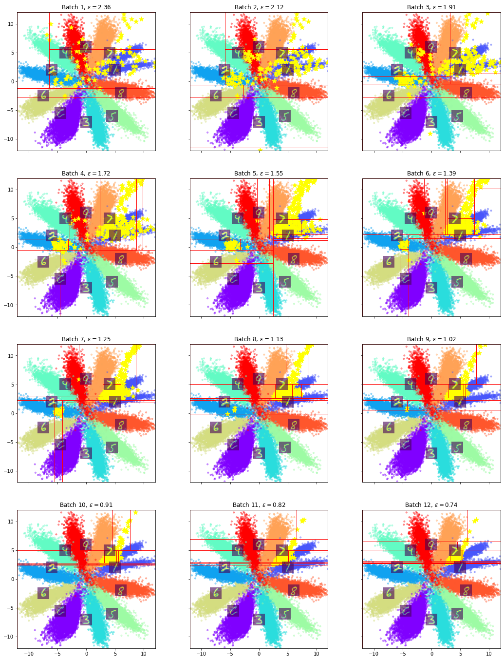
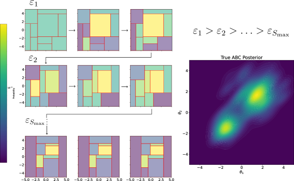
A cartoon of our ABC-Tree algorithm, blending the outer and inner loops into a nested structure, is depicted in Figure 1. Intuitively, the outer loop engulfs the posterior modes through recursive partitioning, and the inner loop pulls boxes with higher reward rates (or higher posterior) more often. The progression of ABC-Tree is visualized in Figure 2 on a two-dimensional example. In a nutshell, active learning algorithms in ABC utilize observations, including proposed parameters and ABC acceptance results, to update the subsequent proposal distribution. In this regard, both the outer and inner loop can be seen as active learning, making the nested algorithm doubly active.
3 ABC Tree
This section unveils our bandit-style ABC approach to learning proposal distributions (and ABC posterior approximations) supported on a finite partition of the parameter space.
3.1 Inner Loop: Bandit ABC
Suppose that the parameter space333We assume that after parameter rescaling, the parameter space is contained in a -dimensional unit cube. Our plots will often be transformed back to the original scale. has been partitioned into (box-shaped) regions . Each region will be regarded as an arm in the multi-arm bandit setting. Playing an arm is equivalent to first drawing a parameter value from inside the box and then generating a fake data vector . Each box is chosen with a probability where and, given , the trial is selected according to . These two steps constitute an ABC proposal distribution
| (3.1) |
defined as the prior which has been rescaled for each bin. The primary goal of the inner loop is to obtain a query-efficient proposal distribution on the arms, given the partition .
Consider a fixed acceptance threshold and a simulation budget . With the objective of sampling from the ABC posterior , at each occasion we select a region and a parameter guess within to observe an ABC acceptance reward
| (3.2) |
We denote the unknown probability of the region (i.e. arm) to yield the reward (3.2) by . At the commencement of the simulation process, we have no information about how likely each region is to yield a reward and we express our uncertainty about through a beta distribution . As the simulation progresses, we learn about ’s by collecting rewards. We leverage this knowledge by updating and as well as bin proposal probabilities for every by prioritizing bins that have a higher success rate. The updating of will be achieved by a Thompson Sampling style routine for binary bandits. Before explaining the updating procedure, it is instrumental to understand how the ABC reward means ’s relate to the projection of the ABC likelihood onto discrete distributions supported on . This crucial insight, presented in the Lemma below, provides a justification for our bandit-style approach.
Lemma 1.
For any region we have
| (3.3) |
where the expectation is taken over the distribution of for .
Proof.
This is due to the definition
This Lemma suggests that one could build a histogram reconstruction of the posterior supported on by averaging over many sampled rewards from each bin and then normalizing them. Sampling each bin separately is inefficient if there are many bins that do not contain a lot of posterior mass. This is why we employ Thompson Sampling style algorithm which focuses on the bins that have enough support. Rather than directly reporting a step function approximation to the ABC posterior, we turn this approximation into an ABC proposal distribution (3.1) built on a partition .
Algorithm 1 summarizes the inner loop of our ABC-Tree method. For each cell , we employ a beta distribution which reflects uncertainty about the value of the marginal likelihood in (2.1) restricted to after iterations. At the beginning of the simulation, we have no information about the likelihood and thereby set . Later, as we obtain a new partition from the outer loop in Section 3.2, we can choose a different initialization and which is based ABC lookup tables from previous loops. After collecting ABC rewards (Algorithm 1 line 9), we can update our beliefs about the likelihood inside by increasing either or (Algorithm 1 line 11). Similarly to other query-efficient ABC techniques, it is important to model the uncertainty in the underlying likelihood [19, 23] and to sample new parameters to reduce this uncertainty (exploration) while, at the same time, increasing the acceptance rate (exploitation). We achieve this balance here though a Thompson Sampling (TS) style procedure using Beta distribution updating.
Recall that, in each round , TS chooses an arm to play based on the largest sampled . The question remains whether such a strategy is compatible with the goal of exploring the entire ABC posterior. Intuitively, for the purpose of ABC posterior sampling, we might want to allow more exploration and choose an arm according to sampling as opposed to optimization. In the effort to learn about the (marginal) likelihood function on , we might want to compute the mean of , as opposed to a random sample. Such can be regarded as an approximation to restricted to . By weighting by the prior , Lemma 1 implies that constitutes an approximation to the ABC posterior on 444Random sampling from the beta distribution as opposed to computing the mean would yield a more noisy approximation. These two strategies, however, were found to perform comparably well.. While the approximation to the discretized posterior encapsulated in alone can be attempted as a proposal for the next step, it might be advisable (as discussed in Section 3.1.2) to further refine this proposal through regularization. Such a refinement, denoted by , is then used to pull an arm through sampling (not optimization) each with a probability .
Since the sampled parameters have been obtained under varying proposals that are different from the prior, we need to revert the samples back to the original prior by importance weighting. The parameter value can be re-weighted by the importance weight which boils down to . For a uniform prior over a compact domain, is simply the reciprocal volume of the box . The importance weight can be also approximated by box frequencies by sampling from a prior.
Remark 1.
(Sampling from ) In practice, it might be difficult to efficiently sample from for priors other than uniform. It might be worthwhile to run ABC-Tree under a step-function approximation to through , where . This prior boils down to uniform sampling inside the box for each arm pull. Each resulting ABC-Tree sample obtained by the inner loop would have to be reweighted by a weight when . The posterior approximation (3.4) would have to undergo suitable reweighting as well.
3.1.1 Adaptive Histogram Posterior Approximation
Recall that each distribution reflects the uncertainty about the value of the marginal likelihood inside . After runs of the algorithm, the mean of this distribution constitutes a reasonable estimator of this value. We can thereby form a step-function approximation to the -posterior (2.2) by playing the bandit game as follows
| (3.4) |
where is the volume of and The approximation to the -posterior mass of is proportional to the product of the prior mass of and the mean ABC reward for the arm . For the uniform prior on we have in which case the volumes cancel each other out and can be normalized to sum to . The quality of the -posterior approximation (3.4) depends on the quality of the partition and its ability to capture local curvatures of the -posterior. Updating occurs in the outer loop of ABC-Tree discussed in Section 3.2. From (3.3) we see that the Algorithm 1 learns a step-wise function that approximates the ABC likelihood (posterior) up to a constant, i.e. we do not require during the computation that the approximation corresponds to a density. This is why we refrain from modeling the arm reward probabilities using a Dirichlet distribution. Note also that the discrete posterior approximation (3.4) is very different from a step-wise approximation that could be obtained after ABC rejections through conjugate updating of a Dirichlet prior distribution (or using Polya Trees) after observing acceptance counts for each bin. Our approach learns from the intermediate ABC rejections by updating the Beta distributions.
3.1.2 Benefits of Regularized Exploitation
For ABC, some proposal distributions are better than others. One can define an optimal proposal for a target distribution , where with respect to a utility function as its minimizer
| (3.5) |
Note that is unknown, and thus is unknown as well. Instead, can be sequentially learned over the course of the ABC simulation process, and can be estimated by given the current estimate at iteration . We primarily concern ourselves with
| (3.6) |
The first one is maximized at , implying that , and so parameters are proposed by sampling from our current model for . This approach has been employed in other likelihood-free inference methods [37, 42]. The second one is the sampling efficiency proposed by Alsing et al. [3], which is another reasonable candidate as its maximization increases the ABC acceptance rate while controlling importance weight variance. At each iteration of the inner loop (Algorithm 1 line 6) we update through the refinement of the posterior estimate via . We regard this projection as regularized exploitation. The purpose of this regularization is to improve the variance of the importance weights by trading-off the ABC acceptance rate and to avoid oversampling areas around the posterior mode (as will be shown in Example 1). Note that the utility can be quite a general criterion. We can also use the criteria in [8, 16], which adopt the KL divergence to define optimality (See, Section C). Since our tree-based partitioning effectively restricts the parameter space to be finite, the maximization in Eq. (3.5) becomes tractable to perform after every subsequent simulation for a variety of choices of .
While the utility of an individual proposal can be measured by , we want to define a measure of effectiveness of an entire inner loop responsible for producing the sequence of proposal distributions used throughout a sampling procedure. Therefore, we introduce a new notion of regret of an ABC algorithm for learning the optimal proposal. The regret of not using the optimal proposal for an approximation to the -posterior can be defined as the following loss in efficiency of the proposal distributions
| (3.7) |
where denotes the algorithm that decides each proposal based on previous information . The expectation is taken over the interaction between the algorithm’s choices , and ABC acceptances . Such a regret can be seen as loosely parallel to the notion of cumulative regret in multi armed bandits (2.3), where the key distinction is that the regret considers the distribution used to propose arms to play rather than only the arm choices and corresponding rewards.
The following theorem says that Algorithm 1 indeed controls the regret for suitable efficiency functions . Note that satisfies the conditions in Assumption 1 for any . In Section A.2, we show that there exists such that satisfies Assumption 1.
Assumption 1.
Let . For all , there exists such that satisfies
| (For upper bound) | |||
| (For upper bound) |
for all , , and
| (For lower bound) |
for all where , and .
Theorem 3.1.
Consider a slightly modified version of Algorithm 1 that employs an initialization phase by first playing each arm times. For defined in (3.2), let be the ABC acceptance rate when sampling from . Let be the prior mass on and let be a set of probability vectors such that when . Denoting the modified algorithm as , we have (for sufficiently large )
where the infimum is taken over all possible strategies for choosing bins .
Proof.
See Section A.1 in the supplement.
The above result highlights that this regularized exploitative approach controls regret at a rate that at most corresponds to a lower bound up to logarithmic factors. Intuitively, maximizing the sampling efficiency for inherently enforces a sufficient amount of exploration, while pushing the proposal distribution closer to the prior in order to control importance weight variance.
Example 1.
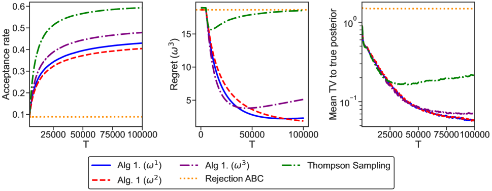
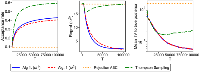
We consider a toy example with a discretized normal likelihood on the parameter space with a uniform prior. In Figure 3, we compare rejection ABC (orange) with four schemes for sequentially updating the proposal distribution. We use Algorithm 1 with each utility function in (3.6) and Thompson Sampling (green). Despite Thompson Sampling having the largest acceptance rate, it is unable to recreate the posterior as the variance of the importance weights becomes large while it eventually over-samples the posterior mode. Rejection ABC has the lowest acceptance rate. Algorithm 1 represents a sweet spot between them. We refer to Section B.1 for details.
3.2 Outer Loop: Adaptive Discretization
The inner loop learns the optimal proposal for a given partition. The ability of the partition to adapt to the shape of the ABC posterior will massively influence the ABC sampling success, as demonstrated in the following example.
Example 2.
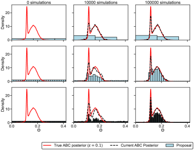
In Figure 4, we consider a toy model with a prior . We display the performance of Algorithm 1 where the parameter space has been partitioned into regular bins. A too-coarse grid (first row) may not be able to eliminate trials in the areas where the posterior is small. On the other hand, a too-fine grid (bottom row) may lead to overfitting [47, 39]. In practice, the optimal grid size depends on the smoothness of the underlying ABC acceptance rate function, and of the intractable likelihood function, which is not known a priori. The middle row presents partitioning which is able to provide a more accurate approximation to the ABC posterior within fewer trials.
The outer loop of ABC-Tree seeks to sequentially discretize the parameter space into hyperrectangles on which to apply Algorithm 1. Each iteration of the inner loop assumes that the ABC tolerance is fixed at . We index the outer loop iterations with and use a sequence of decreasing thresholds , one for each outer loop (analogously to particle-filtering based ABC approaches [44, 8]). Beginning with larger tolerance thresholds allows us to more quickly learn areas of the parameter space that are likely to be relevant at lower tolerance levels, which will be necessary for accurate posterior inference.
We denote the ABC lookup table from the round with
| (3.8) |
where the rewards have been computed on at a chosen threshold (not necessarily ). With we denote the entire history before the round. The goal of the inner loop is to learn a new partition reflecting the allocation of past acceptances at the most recent threshold . This is why we use the training data , recomputing the binary rewards at a level for all preceding rounds. The new partition
| (3.9) |
is chosen according to a rule (distribution) which can be either a delta measure when the partitioning with a deterministic function of the data (such as CART) or random when it represents a sample from a distribution over partitions given . This rule may also depend on the previous partition if it were to be (deterministically) refined by adding more splits. We primarily focus on tree-shaped partitions and discuss various choices of later. A well chosen tree structure will allow us to decipher variability of the acceptance rate by increasing resolution in relevant areas and, at the same time, splitting less often in flat (negligible) likelihood areas.
The ABC-Tree enterprise is visualized in Figure 2. Each row corresponds to an Inner Loop, keeping the partition and the tolerance level fixed. The Inner Loop updates the probability mass of the proposal (and the piecewise constant posterior approximation) within each hyper-rectangle at every iteration . After accepting parameter values, we move onto inner loop at a decreased level and on an updated partition . Note that the parameters and in line 8 and 9 of Algorithm 2 provide an initialization of the mean reward Beta distributions for the Inner Loop based on the rejection information from previous rounds. When updating the partition through (3.9), we employ all of our current information in an extended window approach, in which we construct the partition based on all of our previous data points. As an alternative, one can employ a rolling window style of analysis by restricting the partitioning rule to only depend on the most recent completed outer loop. This is a reasonable choice because as the algorithm progresses, the acceptance threshold becomes smaller, causing the -likelihood to become closer to the true intractable likelihood function. As such, the most recent batch of simulated data is likely to provides a more representative sample of the true posterior than the previous data.
3.2.1 Partitioning Choices
Several options for in (3.8) are available. We consider several options below but this list is by no means exhaustive.
Classification Trees.
We can model the past ABC acceptances using a regularized classification tree obtained by regressing onto for and . Using a pruned tree after cross-validation is a deterministic assignment and will lead to a rough partition which may wrap sharp posterior modes into larger boxes through data-adaptive (non-dyadic) splitting. This strategy will be sufficient for learning an ABC proposal and for obtaining an ABC posterior approximation from the samples after importance re-weightining. This strategy may not necessarily yield an accurate step-function approximation to the posterior (as outlined in Section 3.1.1).
Bayesian Additive Regression Trees.
BART [13] is an ensemble of trees yielding finer partitions (by overlapping many small partitions) with good approximation properties [39] The partitioning function in (3.9) is a random draw from the BART posterior (overlapping partitions for each sampled tree) after a burnin period. While the default strategy in BART is trees, a draw of a forest this large will lead to a very refined partition capable of approximating the acceptance function well but increasing the number of arms to pull in the next round. The optimal number of bins depends on the dimension of as well as the smoothness of the underlying function and the number of data points [39]. Not knowing the optimal number of bins in advance, we recommend to use BART for higher dimensional parameter spaces, which may adaptively finds the optimal number of bins.
Dyadic Partitioning.
Similarly to the hierarchical online optimization algorithm of Bubeck et al. [12], we can bisect the parameter space dyadically at a midpoint along each box. For the compact parameter space , it is easy to compute the volume of each dyadic cell. We can grow a binary tree over the parameter space from a root node by splitting after sufficiently many parameter values have been accepted at the threshold. We split the leaf node in which the largest quantity of parameters were proposed times after each iteration of the outer loop, where may be chosen by the user and may depend on the dimension of the parameter space. In the example below, we set . The dimension in which to split at each depth of the tree can be simply selected sequentially, or by splitting in the direction that best separates accepted from rejected parameter values. This adds a form of variable selection that allows the algorithm to split in dimensions that are more relevant to variation in the acceptance rate within the leaf node.
As an alternative, the dynamic trees of Taddy et al. [45] provide another appealing option for partitioning . Bayesian inference over these trees is accomplished via a particle learning algorithm that is amenable to sequential updating, and a filtered posterior that limits the amount of change with each new observation. For the purpose of ABC posterior sampling, the partition may not need to be fine enough as long as it can successfully direct regions of high-low likelihood. In Table 1 (Supplement Section C.4), we see that our tree ABC can be as fast as SMC-ABC [44, 8] when .
Example 3.
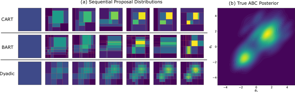
We show the progression of ABC proposals on a simple synthetic example with a mixture of two bivariate isotropic Gaussians. With we observe data from and assume a uniform prior555While here we did not rescale the parameters to be inside , the partitioning idea is the same. for . Figure 5 displays the sequence of partitioning-based proposal distributions using a pruned classification tree (top row), BART (five trees with 1000 burn-in), and dyadic partitioning. As decreases, and we accrue more simulated data, the proposal distributions more closely encapsulates the true ABC posterior.
4 MAP-Tree
Another common goal, besides (ABC) posterior sampling, is computing an actual point estimator. While the posterior mean can be obtained directly through simulation, the sometimes preferred maximum-a-posteriori (MAP) estimator is not immediately available when the likelihood cannot be evaluated. We develop a maximum-a-posteriori (MAP) estimation strategy based solely on simulations from the likelihood, i.e. no likelihood values or gradients are required. Similarly as with ABC-Tree, we build a partition by sequentially refining high-probability areas of the posterior. However, unlike with ABC-Tree, our objective is not to find a proposal for ABC to reflect entire posterior uncertainty but rather to find a partition that can isolate the posterior mode. Below, we describe the inner and outer loops of MAP-Tree designed for this purpose.
4.1 Inner Loop: Best Arm Identification
We consider a fixed, small ‘goal’ tolerance and a fixed budget of evaluations of the simulator. Our objective is to maximize the ABC posterior in (2.2) as accurately as possible under this budget. This can be framed as active learning with a regret
| (4.1) |
where and where is the best guess at after steps. To find an approximation to , we adopt a partitioning perspective similar to ABC-Tree. For a given partition , the goal of the inner loop is minimize the regret (4.1) using a proposal distribution supported on . To find the posterior mode we start with an easier problem. We find a mode of an approximation to based on its projection onto step functions supported on . Based on this projection, defined as with , we attempt to identify the bin index for which is the largest. Namely, we define
We aim to estimate by obtained through playing a bandit game with a goal of minimizing . We estimate , the arm with the maximal perceived average posterior peak according to data accrued over the course of the game. The values depend on the marginal likelihood within that is unknown, which we learn about over time. However, our regret is different from (2.3) and manifests itself as an instance of the best arm identification problem [4]. For this reason, we may also seek to modify the playing strategy to de-emphasize greedy maximization and allocate more effort to differentiating between nearly optimal options.
The inner loop algorithm is presented as Algorithm 3 in Section D. Algorithm 3 essentially operates identically to Algorithm 1 except for the acquisition rule for choosing the next arm given the history. For MAP, we are not concerned with controlling the importance weight variance of our proposal, and instead seek to maximize the prior-weighted ABC acceptance rate. We want to oversample small bins having large estimated average posterior mass and zoom in onto these bins in the following outer loop. Therefore, Algorithm 3 directly takes a maximum , where is the sampled acceptance rate of -th bin. This algorithm is more exploitative as there is no regularization (as discussed in Section 3.1.2) nor is there sampling from a categorical distribution to pick an arm. In contrast with ABC-Tree which chooses an arm by first deterministically estimating the mean rewards and then randomly picking an arm, ABC-MAP instead first samples mean rewards and then picks the best arm based on the magnitude of these rewards.
Alternatively, we can also pull arms according to Top-two Thompson Sampling (TTTS) [40] designed for best-arm identification in the multi-arm bandit problem. By oversampling the arm perceived as second-best, the algorithm has more confidence in identifying the best arm. When using the top-two variant, we pull arm by with probability . With probability , we alternatively repeatedly resample from the posterior model until a different parameter value from the original maximizer is chosen.
The following theorem argues that Algorithm 3 controls the probability of misidentifying the optimal arm in a finite parameter space at a near optimal rate.
Theorem 4.1.
Consider a parameter space partitioned as . Consider a uniform prior on regions for each , and let be the average -posterior mass within . Let and let be the estimate of after simulations using an algorithm . Denote by the Algorithm 3 with . Then, for any there exists a constant such that
where denotes a vanishing sequence as . Moreover, any algorithm must satisfy .
Proof.
See Section A.3 in the supplement.
Theorem 4.1 is a consequence of the analysis of top-two Thompson sampling in Russo [40], and shows that Algorithm 3 identifies the optimal mode at nearly the optimal rate, up to a factor of 2 in the exponent. This factor can be nullified when is chosen with oracle knowledge, or adaptively learned during the course of the algorithm [40].
As an example, in Figure 6, we apply Algorithm 3 with TS and Top-two TS (TTTS) on a toy example with a finite parameter space equipped with a uniform prior. As the algorithm progresses, it proposes the parameter value with maximal -posterior density more frequently and with an increasing rate. For more details, see Section B.3.
4.2 Outer Loop: Adaptive Discretization
The partitioning approach laid out in Section 3.2 may also be applied to the MAP estimation problem. Similarly, we discretize the parameter space into a finite set of bins using a tree-based partitioning scheme. However, unlike for ABC posterior sampling, we prefer finer partitions (such as BART with many trees or CART without too much regularization) that are fine enough to isolate the posterior mode in a small box. To this end, dyadic partitioning based on sequentially refining the box after each Outer Loop round might be preferred.
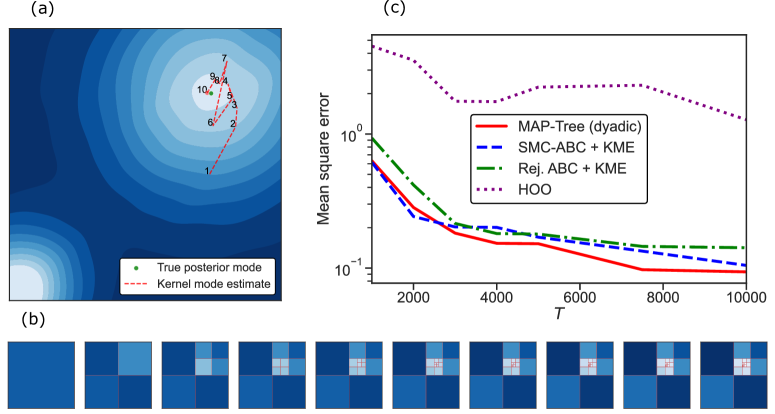
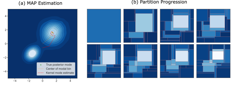
The nested structure of Algorithm 4 for MAP estimation is very similar to Algorithm 2, and is presented in Section D in the Supplement. At the end of the algorithm, the question remains how to estimate the mode . When the dimensionality of the parameter space is not too large, it is feasible to maximize a kernel density estimate of the accepted samples at the final level to estimate the mode of the continuous posterior distribution. One could also treat the center of the bin after several Outer Loops as a point estimate of the mode, and the remainder of the box as a “confidence" region. In Figure 7, we apply Algorithm 4 using dyadic partitioning in the context of Example 3. We can see that the algorithm can closely estimate the true posterior mode with more accuracy than its counterparts. See Section B.4 in the Supplement for more details.
5 Experiments
Recovering an image from an unmasked fraction is an important problem in many machine learning applications [18]. In this section, we focus on the uncertainty quantification of the masked image recovery problem on the MNIST666The MNIST database is a large database of handwritten digits that is commonly used to train various image processing systems. The MNIST database contains grey images with the class (label) information, and is available at http://yann.lecun.com/exdb/mnist/. dataset [30] with deep neural network generative models.
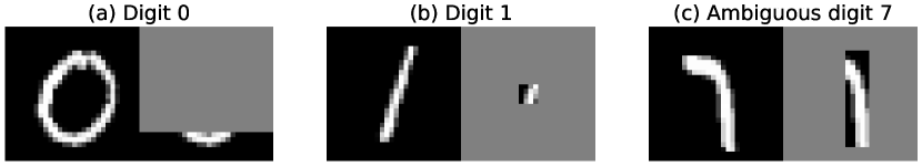
We assume a deterministic image generator , e.g., a decoder, s.t. where and for some , and . Here, the randomness of the image comes from the latent vector , our parameter of interest, and the added noise . As in Figure 8, we observe only a part of data of By using a posterior sample , we can generate possible full images via , For our experiments, we have obtained the generator (decoder) by training an autoencoder with by using the label (digit) information similar to [33, 46], such that each digit number forms a cluster in (see, Figure 10 (a), and for more details, Section B.5).
We experimentally investigate the performance of ABC-Tree (with in (3.6) as the utility function), comparing it to rejection ABC and SMC-ABC as baselines, all running with a budget off simulator evaluations. For MAP estimation, we maximize a kernel density estimate for the baseline methods to estimate the posterior mode, and compare to MAP-Tree. For SMC-ABC and ABC-Tree (and MAP-Tree), we set the tolerance progression rule and quota according to standard heuristics. We note that each method may potentially respond better or worse to different hyperparameter configurations. As a reference distribution, we run rejection ABC for samples, regarding the 1000 samples with lowest discrepancies as an approximated true posterior sample. For the partitioning, we use a classification tree (CART, [10]) with maximum number of leaves bounded by 1000.
5.1 Posterior Sampling
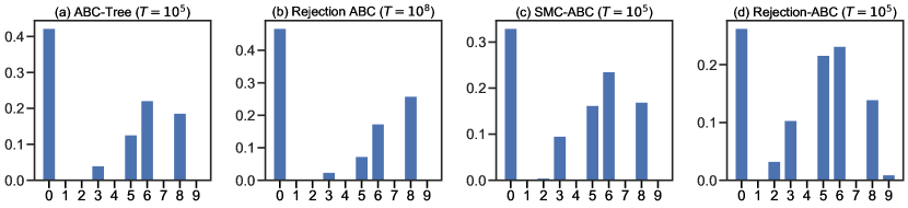
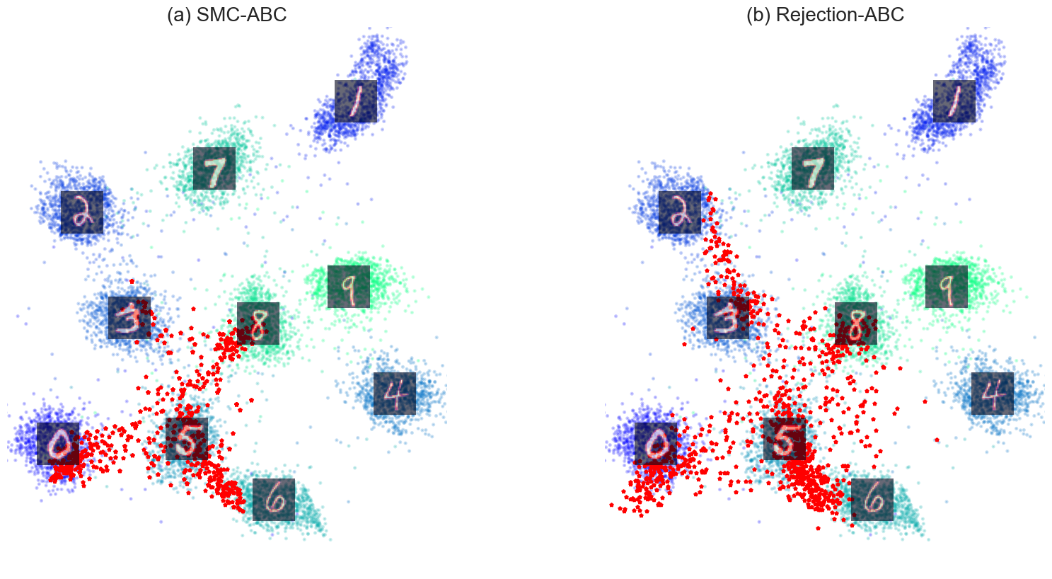
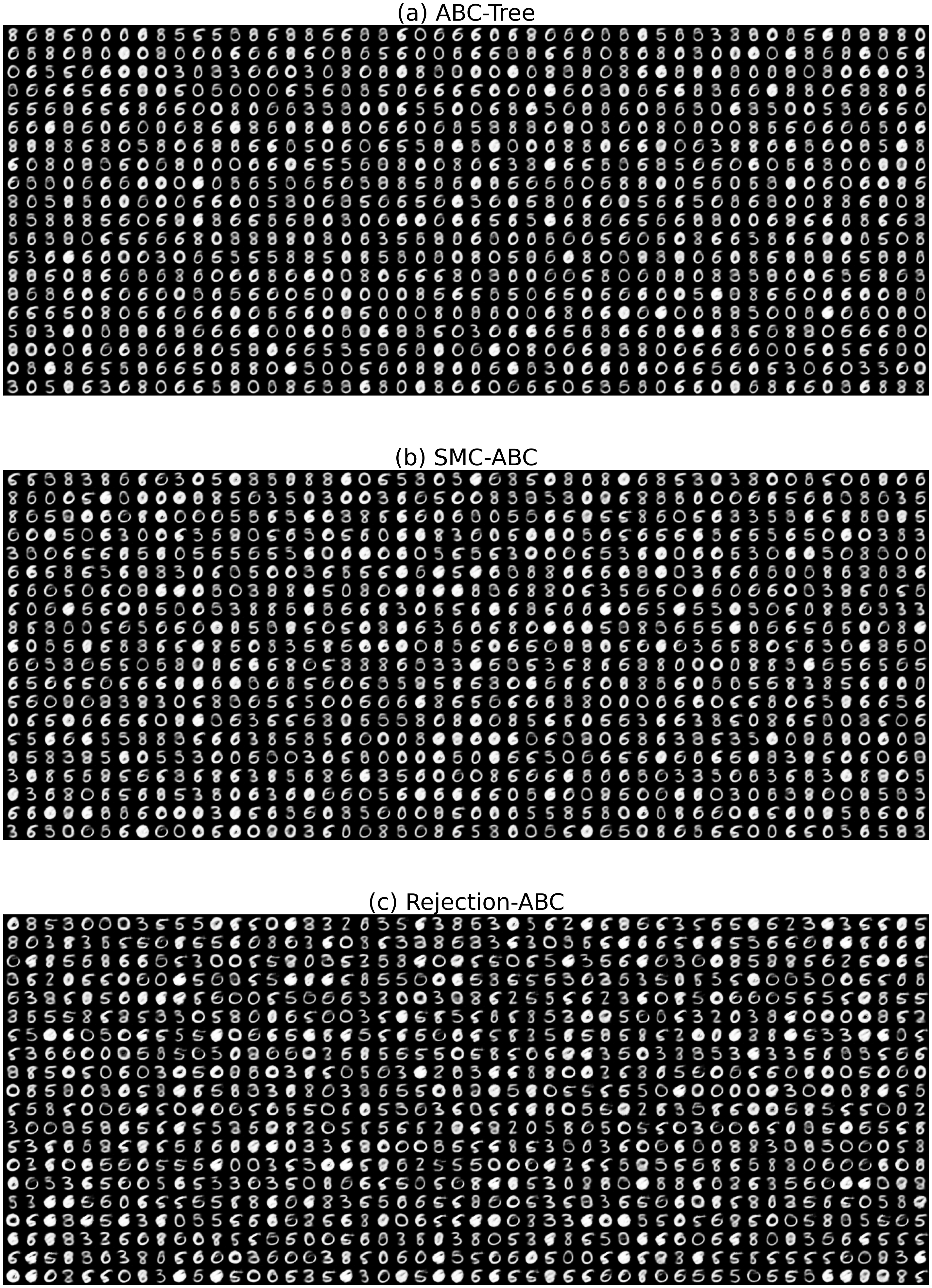
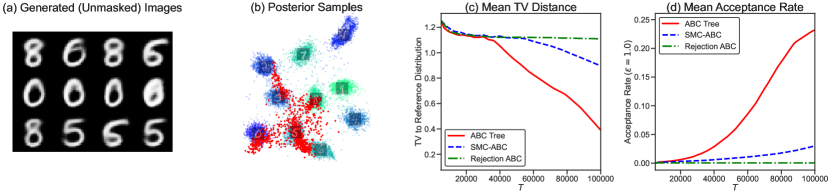
We consider a latent dimension , for which the trained autoencoder provides good reconstruction performance. The prior is set as a uniform distribution over based on the distribution of encoded data in . We mask an image with label 0 as shown in Figure 8 (a), where the visible portion defines . The generated examples by ABC-Tree are shown in Figure 9 (a). The diversity of these numbers implies that the posterior potentially can be multimodal in a five-dimensional space, which may add difficulty when sampling. To see how the sampling process captures such multimodality, we apply iGLoMAP [26], a non-linear dimension reduction technique designed to capture both global and local structure in the data. This two-dimensional visualization in Figure 9 (b) shows that our method catches multimodality in the posterior. Meanwhile, as a proxy for the distance between the reference distribution and the sampled posteriors, we can compute the empirical categorical distribution on the digits , where each generated receives an estimated label by a 10-nearest neighbor classifier trained on the encoded space of the MNIST dataset. Note that as shown in Figure 9 (c), the distance to the reference categorical distribution decreases more rapidly for ABC-Tree than baselines. Furthermore, as in Figure 9 (d), the acceptance rate increases much faster for ABC-Tree (). The categorical distribution of each method for the final 1000 samples is depicted in Figure 17, where the distribution of ABC-Tree () most closely resembles that of rejection ABC with . In Figure 18, we also show a dimension reduction of the baselines. The final 1,000 samples of each method are displayed in Figure 19 in the supplement. Section B.5 provides details on the choice of , the application of iGLoMAP, and the encoded space of MNIST. Section C.3 presents further empirical investigation of ABC-Tree on MNIST regarding the choice of the utility function and the tree size limits.
5.2 Likelihood-free MAP estimation
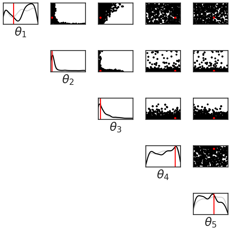
For MAP estimation, we focus on as it allows for visualization of , the posterior samples, and the tree splits as well. The prior is a uniform distribution over to encompass the distribution of encoded data. As with is not sufficient for embedding the MNIST dataset (see, Section B.5), the trained generator can represent only a few stereotypical digit shapes for each number. In this situation, the posterior distribution would resemble a unimodal distribution.
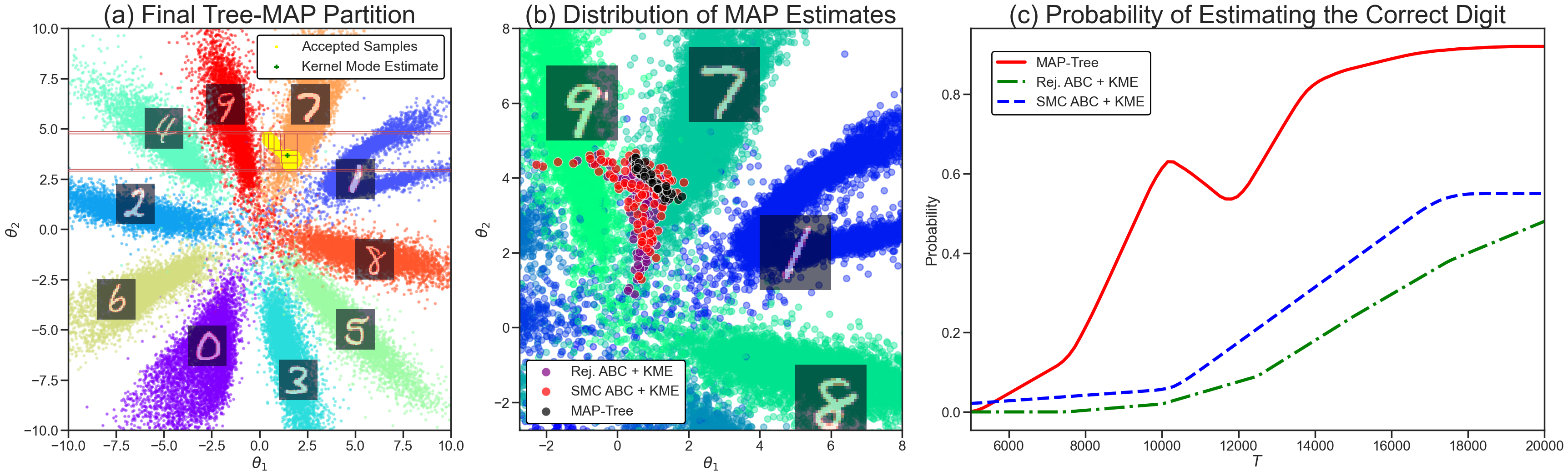
In order to assess our methodology for MAP estimation, we chose an example image where the digit can plausibly be a member in multiple classes. In Figure 8 (c), we see an example of a handwritten digit which resembles a 7, though could plausibly resemble a 9, or a 1. A pilot run of rejection ABC with a large amount () of samples and kernel mode estimation confirms that the (approximated) posterior mode lies in a region of surrounded by data points with label 7. In Figure 10 (a), we see that the final partition used by MAP-Tree zooms in on highly relevant regions in , which are the most likely to produce masked images resembling our observed data. In (b), we visualize the distribution of MAP estimates in for each method over 100 repeated trials, observing a more narrow distribution localized within a region corresponding to the correct digit for MAP-Tree. From each MAP estimate in , we compute the estimated digit by a 10-nearest neighbor classification trained on the encoded original dataset, as in Section 5.1. In (c), we see that over 100 repeated trials, the estimated digits resulting from MAP-Tree are classified as the correct digit 7 with significantly higher probability when compared with baseline ABC methods and kernel mode estimation. The full progression of MAP-Tree on this example can be seen in Figure 20.
6 Concluding Remarks
In this work, we developed a new way of approaching likelihood-free inference and MAP estimation by combining tree partitioning with active learning. This allows us to encourage ABC sampling from the most supported regions of the parameter space. ABC-Tree consists of an outer loop (refining a partition of the parameter space) and an inner loop (refining an ABC proposal on a given partition). We illustrated our approach on a difficult problem of uncertainty quantification over masked image fractions. In Section C in the Supplement, we also provide simulation results on the Heston stochastic volatility model [21] and the Lotka-Volterra model. We believe that our development provides a possible avenue for scaling up ABC to high-dimensional settings, and can potentially inspire further research bridging trees and bandit algorithms.
References
- Agrawal [1995] Rajeev Agrawal. The continuum-armed bandit problem. SIAM journal on control and optimization, 33(6):1926–1951, 1995.
- Agrawal and Goyal [2017] Shipra Agrawal and Navin Goyal. Near-optimal regret bounds for Thompson sampling. Journal of the ACM (JACM), 64(5):1–24, 2017.
- Alsing et al. [2018] Justin Alsing, Benjamin D. Wandelt, and Stephen M. Feeney. Optimal proposals for approximate Bayesian computation. arXiv preprint arXiv:1808.06040, 2018.
- Audibert and Bubeck [2010] Jean-Yves Audibert and Sébastien Bubeck. Best arm identification in multi-armed bandits. In COLT-23th Conference on learning theory, pages 13–p, 2010.
- Auer et al. [2002] Peter Auer, Nicolo Cesa-Bianchi, and Paul Fischer. Finite-time analysis of the multiarmed bandit problem. Machine learning, 47:235–256, 2002.
- Beaumont [2010] Mark A. Beaumont. Approximate Bayesian computation in evolution and ecology. Annual review of ecology, evolution, and systematics, 41:379–406, 2010.
- Beaumont et al. [2002] Mark A. Beaumont, Wenyang Zhang, and David J. Balding. Approximate Bayesian computation in population genetics. Genetics, 162(4):2025–2035, 2002.
- Beaumont et al. [2009] Mark A. Beaumont, Jean-Marie Cornuet, Jean-Michel Marin, and Christian P. Robert. Adaptive approximate Bayesian computation. Biometrika, 96(4):983–990, 2009.
- Black and Scholes [1973] Fischer Black and Myron Scholes. The pricing of options and corporate liabilities. Journal of political economy, 81(3):637–654, 1973.
- Breiman et al. [1984] L. Breiman, Jerome H. Friedman, Richard A. Olshen, and C. J. Stone. Classification and regression trees. Biometrics, 40:874, 1984.
- Bubeck et al. [2009] Sébastien Bubeck, Rémi Munos, and Gilles Stoltz. Pure exploration in multi-armed bandits problems. In Algorithmic Learning Theory: 20th International Conference, ALT 2009, Porto, Portugal, October 3-5, 2009. Proceedings 20, pages 23–37. Springer, 2009.
- Bubeck et al. [2011] Sébastien Bubeck, Rémi Munos, Gilles Stoltz, and Csaba Szepesvári. X-armed bandits. Journal of Machine Learning Research, 12(5), 2011.
- Chipman et al. [2010] Hugh A. Chipman, Edward I. George, and Robert E. McCulloch. BART: Bayesian additive regression trees. The Annals of Applied Statistics, 4(1):266 – 298, 2010.
- Diggle and Gratton [1984] Peter J. Diggle and Richard J. Gratton. Monte Carlo methods of inference for implicit statistical models. Journal of the Royal Statistical Society Series B: Statistical Methodology, 46(2):193–212, 1984.
- Fan et al. [2013] Yanan Fan, David J. Nott, and Scott A. Sisson. Approximate Bayesian computation via regression density estimation. Stat, 2(1):34–48, 2013.
- Filippi et al. [2013] Sarah Filippi, Chris P. Barnes, Julien Cornebise, and Michael P.H. Stumpf. On optimality of kernels for approximate Bayesian computation using sequential Monte Carlo. Statistical applications in genetics and molecular biology, 12(1):87–107, 2013.
- Frühwirth-Schnatter and Sögner [2003] Sylvia Frühwirth-Schnatter and Leopold Sögner. Bayesian estimation of the Heston stochastic volatility model. In Operations Research Proceedings 2002: Selected Papers of the International Conference on Operations Research (SOR 2002), Klagenfurt, September 2–5, 2002, pages 480–485. Springer, 2003.
- Garnelo et al. [2018] Marta Garnelo, Dan Rosenbaum, Christopher Maddison, Tiago Ramalho, David Saxton, Murray Shanahan, Yee Whye Teh, Danilo Rezende, and SM Ali Eslami. Conditional neural processes. In International conference on machine learning, pages 1704–1713. PMLR, 2018.
- Gutmann and Corander [2016] Michael Gutmann and Jukka Corander. Bayesian optimization for likelihood-free inference of simulator-based statistical models. Journal of Machine Learning Research, 17(125):1–47, 2016.
- Hennig and Schuler [2012] Philipp Hennig and Christian J. Schuler. Entropy search for information-efficient global optimization. Journal of Machine Learning Research, 13(6), 2012.
- Heston [1993] Steven L. Heston. A closed-form solution for options with stochastic volatility with applications to bond and currency options. The review of financial studies, 6(2):327–343, 1993.
- Hore et al. [2010] Satadru Hore, Michael Johannes, Hedibert Lopes, Robert McCulloch, and Nicholas Polson. Bayesian computation in finance. Frontiers of Statistical Decision Making and Bayesian Analysis, pages 383–396, 2010.
- Järvenpää et al. [2018] Marko Järvenpää, Michael U. Gutmann, Aki Vehtari, and Pekka Marttinen. Gaussian process modelling in approximate Bayesian computation to estimate horizontal gene transfer in bacteria. The Annals of Applied Statistics, 12(4):2228–2251, 2018.
- Järvenpää et al. [2019] Marko Järvenpää, Michael U. Gutmann, Aki Vehtari, and Pekka Marttinen. Efficient acquisition rules for model-based approximate Bayesian computation. Bayesian Analysis, 14(2):595–622, 2019.
- Kandasamy et al. [2017] Kirthevasan Kandasamy, Jeff Schneider, and Barnabás Póczos. Query efficient posterior estimation in scientific experiments via Bayesian active learning. Artificial Intelligence, 243:45–56, 2017.
- Kim and Wang [2024] Jungeum Kim and Xiao Wang. Inductive global and local manifold approximation and projection. under review, 2024.
- Kleinberg [2004] Robert Kleinberg. Nearly tight bounds for the continuum-armed bandit problem. Advances in Neural Information Processing Systems, 17, 2004.
- Kleinberg et al. [2008] Robert Kleinberg, Aleksandrs Slivkins, and Eli Upfal. Multi-armed bandits in metric spaces. In Proceedings of the fortieth annual ACM symposium on Theory of computing, pages 681–690, 2008.
- Lattimore and Szepesvári [2020] Tor Lattimore and Csaba Szepesvári. Bandit algorithms. Cambridge University Press, 2020.
- LeCun et al. [2010] Yann LeCun, Corinna Cortes, and C.J. Burges. MNIST handwritten digit database. AT&T Labs [Online]. Available: http://yann. lecun. com/exdb/mnist, 2:18, 2010.
- Li and Hannig [2020] Gang Li and Jan Hannig. Deep fiducial inference. Stat, 9(1):e308, 2020.
- Lueckmann et al. [2019] Jan-Matthis Lueckmann, Giacomo Bassetto, Theofanis Karaletsos, and Jakob H. Macke. Likelihood-free inference with emulator networks. In Symposium on Advances in Approximate Bayesian Inference, pages 32–53. PMLR, 2019.
- Makhzani et al. [2015] Alireza Makhzani, Jonathon Shlens, Navdeep Jaitly, Ian Goodfellow, and Brendan Frey. Adversarial autoencoders. arXiv preprint arXiv:1511.05644, 2015.
- Marjoram et al. [2003] Paul Marjoram, John Molitor, Vincent Plagnol, and Simon Tavaré. Markov chain Monte Carlo without likelihoods. Proceedings of the National Academy of Sciences, 100(26):15324–15328, 2003.
- Martin et al. [2019] Gael M. Martin, Brendan P.M. McCabe, David T. Frazier, Worapree Maneesoonthorn, and Christian P. Robert. Auxiliary likelihood-based approximate Bayesian computation in state space models. Journal of Computational and Graphical Statistics, 28(3):508–522, 2019.
- Meeds and Welling [2014] Edward Meeds and Max Welling. GPS-ABC: Gaussian process surrogate approximate Bayesian computation. arXiv preprint arXiv:1401.2838, 2014.
- Papamakarios et al. [2019] George Papamakarios, David Sterratt, and Iain Murray. Sequential neural likelihood: Fast likelihood-free inference with autoregressive flows. In The 22nd international conference on artificial intelligence and statistics, pages 837–848. PMLR, 2019.
- Polson and Sokolov [2023] Nicholas G Polson and Vadim Sokolov. Generative AI for Bayesian computation. arXiv preprint arXiv:2305.14972, 2023.
- Ročková and Van der Pas [2020] Veronika Ročková and Stephanie Van der Pas. Posterior concentration for Bayesian regression trees and forests. The Annals of Statistics, 48(4):2108–2131, 2020.
- Russo [2016] Daniel Russo. Simple Bayesian algorithms for best arm identification. In Conference on Learning Theory, pages 1417–1418. PMLR, 2016.
- Schafer and Freeman [2012] Chad M. Schafer and Peter E. Freeman. Likelihood-free inference in cosmology: Potential for the estimation of luminosity functions. In Statistical Challenges in Modern Astronomy V, pages 3–19. Springer, 2012.
- Sharrock et al. [2022] Louis Sharrock, Jack Simons, Song Liu, and Mark Beaumont. Sequential neural score estimation: Likelihood-free inference with conditional score based diffusion models. arXiv preprint arXiv:2210.04872, 2022.
- Shephard [2020] Neil Shephard. Statistical aspects of arch and stochastic volatility. In Time series models, pages 1–68. Chapman and Hall/CRC, 2020.
- Sisson et al. [2007] Scott A. Sisson, Yanan Fan, and Mark M. Tanaka. Sequential Monte Carlo without likelihoods. Proceedings of the National Academy of Sciences, 104(6):1760–1765, 2007.
- Taddy et al. [2011] Matthew A. Taddy, Robert B. Gramacy, and Nicholas G. Polson. Dynamic trees for learning and design. Journal of the American Statistical Association, 106(493):109–123, 2011.
- Tolstikhin et al. [2017] Ilya Tolstikhin, Olivier Bousquet, Sylvain Gelly, and Bernhard Schoelkopf. Wasserstein auto-encoders. arXiv preprint arXiv:1711.01558, 2017.
- Van Der Pas and Ročková [2017] Stéphanie Van Der Pas and Veronika Ročková. Bayesian dyadic trees and histograms for regression. Advances in Neural Information Processing Systems, 30, 2017.
- Wang and Ročková [2022] Yuexi Wang and Veronika Ročková. Adversarial Bayesian simulation. arXiv preprint arXiv:2208.12113, 2022.
- Wilkinson [2014] Richard Wilkinson. Accelerating ABC methods using Gaussian processes. In Artificial Intelligence and Statistics, pages 1015–1023. PMLR, 2014.
[appendix] \printcontents[appendix]l1
Appendix Table of Contents
Appendix A Proof of Theorems
A.1 Proof of Theorem 3.1
Setting and notation.
Denote the simplex on elements as . Consider a -armed bandit setup with Bernoulli reward distributions with means . represents our ABC acceptance rate, where , and thus also our unnormalized -likelihood. Let be the uniform prior, for . Define
for . Thus represents the target posterior distribution on our parameter space. Let the function denote the optimal proposal distribution for posterior and optimality criterion , given by . We characterize a problem instance by . We define the regret of algorithm on problem instance after iterations as
where the expectation is with respect to the probability measure induced by the interplay of algorithm and problem instance . The notation mirrors that of the canonical bandit environment defined in Lattimore and Szepesvári [29].
Theorem A.1.
Consider a slightly modified version of Algorithm 1 that employs an initialization phase by first playing each arm times. For defined in (3.2), let be the ABC acceptance rate when sampling from . Let be the prior mass on and let be a set of probability vectors such that when . Denoting the modified algorithm as , we have (for sufficiently large )
where the infimum is taken over all possible strategies for choosing bins .
Proof.
We will first prove the upper bound, and later the lower bound.
Upper Bound
First, note that as (and ). This is because Lemma A.1 ensures that each arm is played atleast a constant (independent of ) fraction of times, ensuring for all and in turn . This implies that for sufficiently large , there exists such that implies . Define .
We now apply Assumption 1 and decompose the regret into that which occurred up to round , and that which occurred after.
We may bound the second term as
using Lemma 2, and the fact that is distributed as the sample mean of Bernoulli random variables with mean . If , the th term in the sum will be 0 for every . We proceed to consider when , and thus . In such cases, we have
using Lemma A.1. Therefore, summing over , we have
for sufficiently large (in particular, ). Therefore, this second term is upper bounded as
and thus
as desired.
Lower bound
First consider the instance in given by , where is the uniform prior and the mean acceptance rates are given by . Now fix any algorithm , and choose . Because , we know that necessarily
We then define a second instance in where , where
adding a small to the th position in the vector, and slightly decreasing all other coordinates proportionately to maintain a norm of . We denote and similarly. As a result of Assumption 1, letting denote the proposal employed by , we have
This can be lower bounded as
Let and be the probability measures on the data resulting from of the interplay of algorithm and reward distributions , respectively. We upper bound the KL-divergence between these measures as
Choosing thus implies that the two bandit environments and are indistinguishable. This implies via a two-point argument that the regret has lower bound
∎
Lemma 2.
For any nonzero vectors , we have
Proof.
We have
∎
Lemma 3.
After an initialization phase of size for each arm, for all , we have
| (A.1) |
Proof.
First, fix and fix . Let denote the (random) number of times arm was played up to time . Due to initialization, we have with probability 1. We first bound the tail probability as
Defining
we observe is a bounded random variable with , and . Thus, a Chernoff-Hoeffding bound yields
for sufficiently large (in particular, for ). Thus
Since this holds for all , and for all with probability 1, we may also conclude
for all .
Let , and note that . Next, we bound
where . Finally, we combine these results to yield
∎
A.2 Special Case of Utility Function
Here, we study the utility of a proposal distribution by its sampling efficiency [3]
where terms in the denominator are defined to be whenever . Because of this, it is clear that will set for each zero , and it suffices to consider only the support of when has zero entries.
We show that Assumption 1 holds for this particular choice of under a uniform prior , with a modified family discrete probability measures that imposes the additional restriction that each nonzero is bounded below by a universal constant .
Lemma 4.
For any posterior there exist constants , such that for any ,
Proof.
Note is twice continuously differentiable in , and is maximized at subject to the constraint
Expanding around some point yields
Second order necessary conditions for constrained optimization imply that satisfies and for any . This yields the desired result, as
for . The dependent constant may be replaced with a universal constant by taking the supremum, which is bounded above due to the assumption . ∎
Lemma 5.
For any fixed , the function is locally Lipschitz in . That is, there exist constants such that
for all .
Proof.
First, we note that in [3], it is shown that can be expressed by the implicit equation
| (A.2) |
where is given by
Thus, the functional form for the optimal proposal is known explicitly except for the value of the scalar , and given , it is uniquely determined by . Rearranging, we can express with the implicit equation
equivalently written as
Note that , and observe that
which is always positive. Thus, the implicit function theorem yields that for any fixed , there exists and a unique twice continuously differentiable function such that .
If we now denote to be a function defined by Equation A.2 with replacing , we can note that is twice continuously differentiable in and , and that . Therefore, the function is twice continuously differentiable for . Thus, we have for any ,
The -dependent constant may be replaced with a universal constant by taking the supremum, once again as . ∎
Lemma 6.
There exist constants such that for any and , we have .
Proof.
We will show that the function , defined by
has a negative definite Hessian for sufficiently close to . A short calculation yields that
and for any such that , we have
This implies that there exists a constant such that
To make this hold for in a neighborhood around , we note that the function is twice continuously differentiable with respect to around , which implies that
for all for some . Thus, there exists some , such that for all , for all , we have
∎
Lemma 7.
The function is locally invertible around , and thus the inverse is locally Lipschitz.
Proof.
We consider the implicit function
observing that calculation yields
Note that both are invertible. Applying the implicit and inverse function theorems yields the existence of such that for any , the (implicitly defined) function is bijective. Furthermore, since we argued is locally Lipschitz with constant , then there exists such that for , the inverse function of is Lipschitz with constant . ∎
A.3 Proof of Theorem 4.1
Setting
Consider a problem instance defined by vector of ABC acceptance rates and prior distribution . Thus, we have the ABC posterior defined via for . Let and let be the estimate of the maximal after simulations using Algorithm . Denote Algorithm 3 with the choice as .
There exists an instance dependent constant such that , where denotes a vanishing sequence as .
Proof.
The likelihood-free MAP estimation setting with a uniform prior on a finite parameter space can be characterized as an instance of the best-arm identification problem in multi-armed bandits. Each arm is a parameter in the parameter space, with reward distribution given by , where is the mean ABC acceptance rate when proposing parameters from parameter . Since the ABC acceptance rate is proportional to the -likelihood (Lemma 1), identifying the arm with maximal mean reward in the bandit setup is equivalent to identifying the parameter value with maximal -likelihood.
Theorem 1 of Russo [40] may then be applied to obtain the desired result.
∎
Appendix B Implementation Details
B.1 Empirical Regret Comparison
We consider a toy example on a discrete parameter space , where we treat each plausible parameter value as a bin . The ABC likelihood is defined via and . We consider a uniform prior on . We apply standard rejection ABC as a baseline, proposing parameters from the prior. We sequentially update the proposal distribution using four schemes: Algorithm 1 using each function in (3.6), and Thompson Sampling (picking an arm with the largest sampled value from beta distributions). We report the acceptance rate, regret (using ) as well as the TV distance to the true posterior in Figure 3. Despite Thompson Sampling having the largest acceptance rate, it is unable to recreate the posterior as well as other approaches as the variance of the importance weights become large as it eventually starts to oversample the posterior mode. Rejection ABC has the lowest acceptance rate. Algorithm 1 represents a sweet spot between them. The three variants of Alg. 1 employ different choices of utility functions , that prioritize having a high acceptance rate at varying levels. Prioritizing a higher acceptance rate may increase performance in the shorter term, as it helps the algorithm to progress to a lower level sooner, but may eventually result in importance weights with high variance as the nearly modal areas could be oversampled.
B.2 Tree Regression (CART)
To fit the trees from which the proposal distributions are made, we use a classification tree (in the style of CART) with a fixed maximum depth, number of leaves, and a minimum number of samples per leaf in order to prevent overfitting to the noisy data. For our experiments, we set the maximum number of leaves to be 1000 and the minimum number of samples per leaf to be 10.
B.3 Details of Figure 6
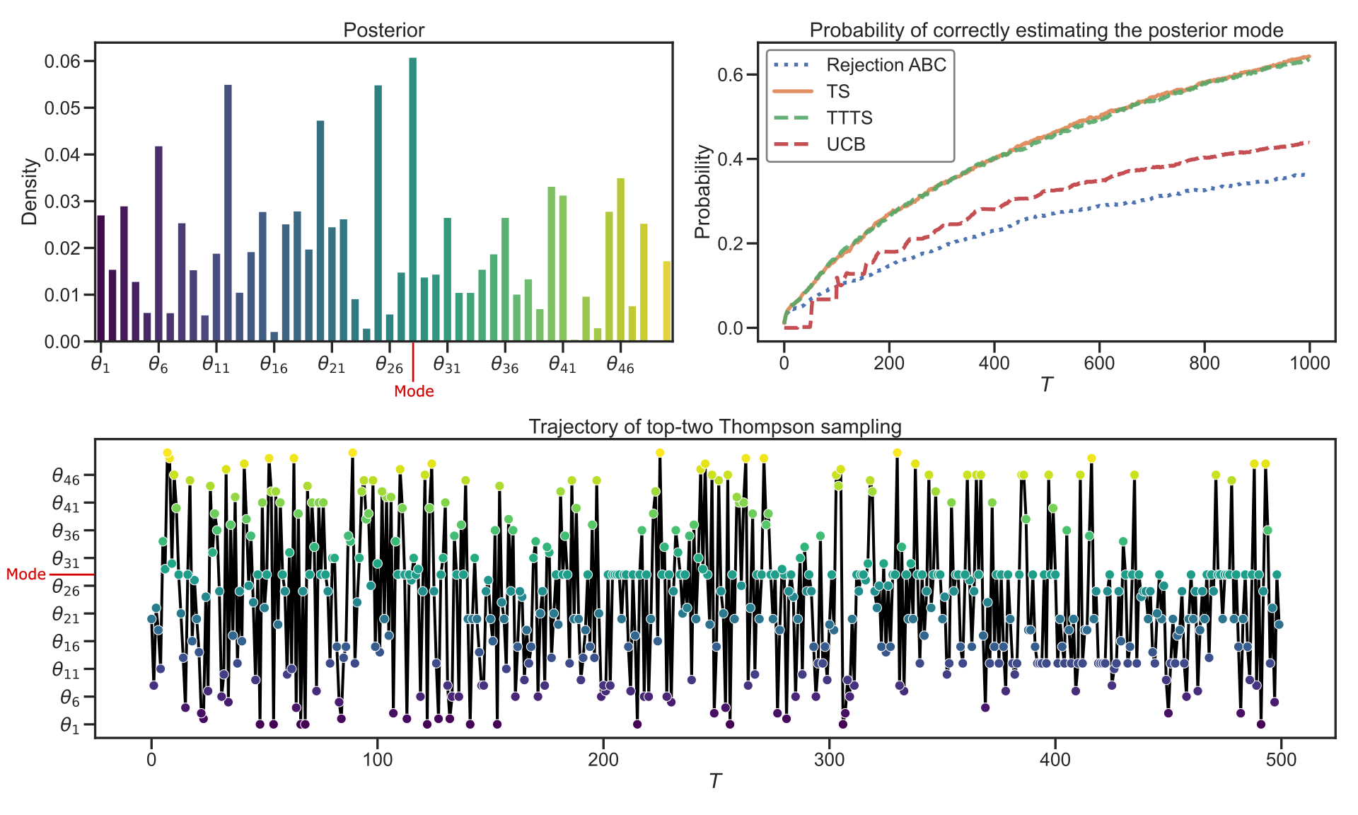
We apply Algorithm 3 with TS and Top-two TS (TTTS) on a toy example with a finite parameter space equipped with a uniform prior. In Figure 6, the upper left shows the -posterior values (normalized mean ABC acceptance rate for each parameter value). In this example, the difficulty arises from the fact that several other parameter values exhibit posterior mass nearly as high as that of the mode . In the upper right plot in Figure 6, we estimate the posterior mode by the arm with maximal estimated posterior mass, and compare our TS procedures with rejection ABC (and maximization), and the upper confidence bound (UCB) algorithm [5] (treating the ABC acceptance as a binary reward), displaying the empirical probability of correctly identifying the mode over iterations. We observe that Algorithm 3 can identify the true -posterior mode more frequently than other methods, as it obtains more information about the nearly-modal parameter values. The trajectory of the algorithm’s choices in each round for one given sample path is displayed on the bottom in Figure 6. As the algorithm progresses, it proposes the parameter value with maximal -posterior density with an increasing rate.
B.4 Details of Figure 7
In Figure 7, we apply Algorithm 4 using a dyadic partitioning on the bivariate Gaussian mixture toy example from Example 3, with a total budget of simulator evaluations. As we can see, the higher resolution areas in the partition concentrate near the posterior mode, and the algorithm can closely estimate the true posterior mode under a small budget. An analogous example where the partitioning is done via classification trees can be found in Figure 16 in Section C.4, where we observe similar behavior. We compare performance on estimating the posterior mode in terms of squared error, taking the mean over 100 iterations. We compare against rejection ABC and SMC-ABC with kernel mode estimation, as well as the hierarchical online optimization algorithm (HOO) of Bubeck et al. [12]. HOO is an algorithm designed for minimizing cumulative regret in bandit setting with a continuous arm space. The algorithm is a variant of the UCB algorithm that employs a dyadic partitioning using a binary tree on a measurable space. We set , and use acceptance at a fixed as a binary reward. We observe that MAP-Tree can estimate the posterior mode with more accuracy than its counterparts.
B.5 Details of the MNIST Experiment in Section 5
For training an autoencoder on MNIST, a common choice for is between 5 to 10. For us, to obtain a reference distribution through the standard rejection ABC with a reasonable number of simulations , we choose the smallest dimension, that is, we consider for the posterior sampling.
We train an autoencoder by using the Wasserstein autoencoder [46] with noise . Note that an autoencoder involves two neural networks, a decoder and an encoder . We can apply to each MNIST digit image so that . Often, this space (or collectively ) is called a latent space in the generative model literature. When training the autoencoder, we also add a label (digit) information during the optimization process similar to [33] so that the latent space forms a cluster for each digit number in as in Figure 10 (a).
For visualization, we train iGLoMAP’s dimensional reduction mapper that reduces the 5-dimensional parameter vectors () to 2-dimensional vectors. The mapper is a standard feedforward deep neural network. To save the training time, we train the network on 8,000 points of , and then we map our generated and as well for all 60,000 training images of MNIST.
Appendix C Additional Experiment Results and Details
In this section, we present additional results from our method on various other likelihood-free inference models. We include a comparison between optimizing various optimality criteria, including and as well as a third utility function . We define
| (C.1) |
which depends not only on the posterior , but on the acceptance rates in each bin at tolerance . This criterion seeks to regularize maximizing the log acceptance rate of by ensuring that cannot stray too far from . It performs very well initially due to a large acceptance rate, but later may begin to oversample the nearly modal areas once a sufficiently low tolerance has been reached. When using as the utility criterion in Algorithm 2 and Algorithm 1, we compute by , our current model for the acceptance rate from region .
C.1 Heston Stochastic Volatility Model Simulation
In quantitative finance, modeling the dynamics of asset prices is fundamental tool for risk management, trading, and investment strategies. The Heston model is a mathematical framework used to describe the evolution of financial market prices, particularly focusing on the stochastic volatility of an asset [21]. Introduced by Steven Heston in 1993, it allows for more realistic modeling of the volatility surface in options pricing compared to models that assume constant volatility, like the Black-Scholes model [9]. Bayesian analysis has been considered for posterior inference in stochastic volatility models, but has been traditionally challenging [43, 17, 35]. Typical approaches to Bayesian inference in the Heston model involve an exact approach using MCMC [17] and related particle filtering and sequential importance sampling methods [22].

The Heston model describes the dynamics of an asset’s current price as
| (C.2) |
where denotes the risk-free interest rate, denotes the volatility of the asset’s price, and is a Wiener process governing stochastic fluctuations in price. The volatility is assumed to follow an Ornstein-Uhlenbeck process where is another Wiener process. This may alternatively be written as the square-root process on the variance
| (C.3) |
where and have correlation .
We can simulate asset prices according to the Heston model by discretizing the dynamics (C.2) and (C.3) in the above system of stochastic differential equations. The model is parameterized by . We choose the following summary statistics of the simulated asset price time series: mean of log returns, mean of squared log returns, log standard deviation of log returns, log standard deviation of squared log returns, autocorrelation of squared log returns at lag 1, autocorrelation of squared log returns at lag 2, correlation of log returns and squared log returns. These summary statistics were shown to be effective for ABC in stochastic volatility models by Martin et al. [35]. We apply our ABC-Tree method to sample from the posterior of the Heston model. We consider a risk-free interest rate of and initial asset price . As our observed data, draw a sample of 2000 discrete time steps each from a discretization of (C.2) and (C.3). The prior for is given by
The initial results are in Figure 11. We find that the sequential learning performed in ABC-Tree can allow for a more efficient proposal distribution to be learned faster. This leads to improved performance relative to typical ABC methods when under a budget of simulator evaluations. Our method trades off approximation accuracy of the posterior in exchange for the ability to sequentially learn from previous simulations. When the number of simulations becomes very large, any methods that progressively learn a proposal distribution would have also amassed enough data to have a good approximation of the posterior. In such cases, we posit that differences in performance relate more to the difference in approximation accuracy between the method for modeling the likelihood (or posterior), and in the optimality criterion by which the proposal distribution is calculated. For example, on smooth, unimodal densities, the KDE proposal of SMC-ABC may better approximate the optimal proposal, while the tree-based proposal used by ABC-Tree may better approximate the optimal proposal for problem instances with varying levels of local smoothness or posteriors resembling a step function. We also find empirically that Tree ABC appears to outperform SMC-ABC especially well when the parameter space is higher dimensional.
C.2 Lotka-Volterra Model
The Lotka-Volterra predator-prey model is commonly used in ecology to model the dynamics of the populations of two species interacting as predatory and prey. Letting denote the population of the prey and the population of predators, the growth rates of the two species are modeled by the ordinary differential equations and , which are parameterized by the four-dimensional vector . Within the model, prey are assumed to reproduce at an exponential rate in absence of predators, and their rate of decrease is proportional to the product of their population with that of the predators. On the other hand, the population of predators increases proportionally to this product, and decays exponentially. We simulate from the model as a Markov jump process, where the populations are recorded at discrete time steps with exponentially-distributed random wait times.
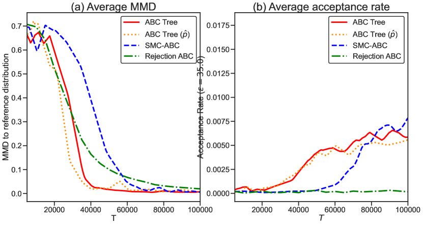
C.3 Additional MNIST Experiment (Image Unmasking)

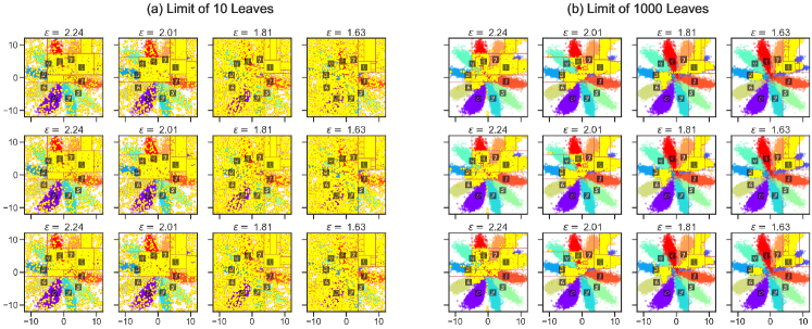
We also include an additional demonstration for the MNIST image unmasking experiment, in which we include a comparison of various functions. In Figure 13, which compares the convergence speed to the estimated true distribution across different optimality criteria. In this experiment, biasing the choice of criterion to favor a larger acceptance rate allows the algorithm to more quickly approximate the posterior at a small . In addition, to visualize the effect of different tree size limits, we consider and impose a maximum of 10 and 1000 leaves, in Figure 14. We can see that the progression is similar, with the samples concentrated near the posterior modes for both cases. However, with a maximum of 10 leaves, the distinction between less important and moderately important areas is less clear, yielding some parameters spread across low posterior regions. On the contrary, the tree approximation with a maximum of leaves is much sharper, with proposed parameters concentrated near multiple local modes.
C.4 Additional Table and Figures
Table 1 shows a comparison of the computational cost for various active learning ABC strategies, including SMC-ABC, where is the total number of iterations across the batches, is the dimensionality of the parameter space, is the maximum number of hyper-rectangles in a partition, and is the number of acceptances before moving to the subsequent tolerance level. The cost when determining the partition depends on the method used, and the entry in the table reflects that of CART. ABC-Tree using either CART or dyadic partitioning has a lower cost than SMC-ABC when .
| Strategy | Cost per tolerance level | Cost per simulation | Total cost |
|---|---|---|---|
| ABC-Tree (CART) | |||
| ABC-Tree (Dyadic) | |||
| SMC-ABC | |||
| Rejection ABC |