Classification of the Mott gap

Abstract

In this paper, we demonstrate the classification of the gap in a holographic setup by studying the density of states. A gap can be classified into order gap and Mott gap depending on the presence of the order due to the symmetry breaking or not. A Mott insulating gap appears in the fermion spectrum due to the strong Coulomb interaction between the electrons. We then classify all Mott gaps as well as order gaps in one-flavor and two-flavor fermions. We also identified possible non-minimal interactions that may produce a flatband.

1 Introduction

The understanding of strongly correlated systems still remains mysterious because of the lack of tools to calculate strange behaviors of materials RevModPhys.78.17 although many useful methods were developed including the dynamical mean-field theory (DMFT) RevModPhys.68.13 to get the modification from the many-body effect. One of the celebrated features of strongly interacting systems is the Mott gap, which can not be described by the gap induced by the order and symmetry breaking. It is induced by the electron-electron on site interaction. Mott physics may be essential in understanding the physics of high-temperature superconductivity since the latter is considered as a doped Mott insulator PhilipNature . Its physics can be best represented by the Hubbard Hamiltonian RevModPhys.40.677 that involves the competition between hopping and on-site repulsion. Although the Hubbard model is not solved completely in two and higher dimensions, the Mott gap is known to be well explained by DMFT RevModPhys.68.13 . The gap appears when onsite repulsion is dominating the hopping.

Gauge/gravity duality Maldacena:1997re ; Gubser:1998bc ; Witten:1998qj provides an alternative tool to study a strongly coupled system with the help of weakly interacting theory of gravity in one higher spatial dimension HKMS ; Seo:2016vks ; Oh:2021xbe ; Song:2019asj ; Oh:2020cym ; Oh:2018wfn ; Seo:2017oyh ; Seo:2017yux . The application of this duality in condensed matter physics has been widely used in the past decade. Since gravity models map strongly coupled boundary field theory, one obvious inquiry is to find a holographic setup. Since DMFT is used to explain the Mott gap, another inquiry is to find an alternative mean field theory for a strongly coupled system. Recently, an alternative mean field theory for a strongly coupled system has been proposed using a holographic approach in Sukrakarn:2023ncp . The main task is to find a gap-like feature without any symmetry breaking in the holographic setup. This is only possible when we consider non-minimal coupling between the gauge and fermionic fields. Because such holographic theory aims at the general theory for strongly interacting system, it would be interesting to exlain the Mott physics in holographic mean field theory and compare with the DMFT. Along this line of thinking, the Pauli interaction term has been utilized in the holographic literature PhysRevLett.106.091602 ; PhysRevD.83.046012 ; PhysRevD.90.044022 ; philip3 ; Seo_2018 . However, the spectral function of the holographic fermion with Pauli interaction has higly asymmetric gap in the sense that uppper side of the Fermi sea has gap but lower side of FS is touched by a spectral peak line, which is clear in spectral function as well as the density of states (DoS). From the DoS in the presence of the dipole coupling, the Mott gap in this theory is ‘soft’ as well as asymmetric. On the other hand, the typical DMFT calculation shows that the Mott gap is symmetric. This motivates us to consider other non-minimal interactions between the gauge field and fermion. Finding a symmetric Mott gap in the DoS analysis of the holographic fermion is the main motivation of this paper. In doing this we can classify Mott gaps as well as the ordered gaps.

In this paper, we first reproduced all the spectral functions for the dipole interaction. We then analyzed the DoS corresponding to the spectral functions, which has not been done in the literature. We then propose our holographic setup with different interactions. From the holographic mean field theory Sukrakarn:2023ncp , we know that only (pseudo) scalar type Yukawa interaction can give a proper gap, while we also know that there should not be any order parameter field involved in the description of the Mott gap. Then the only field we can use is the gauge field describing the density effect and the only way to form a gauge invariant scalar out of the gauge field is $F_{\mu\nu}F^{\mu\nu}$ so that we should try a few version of the $F^{2}{\bar{\psi}}\Gamma^{scalar}\psi$ term. This is the idea of the paper and as a consequence of adding such interaction, we get symmetric Mott gap from some of them. Then, the dependence on temperature, chemical potential, coupling constant, and the effect of fermion mass have been discussed in detail. From the boundary point of view, the possible gamma scalar are $\Gamma^{scalar}=\mathbb{I}_{4},\Gamma^{z},i\Gamma^{5},i\Gamma^{5z}$. This analysis is extended to the two-flavor fermion case. For completeness, we revisit all ordered gaps in holographic setups. Finally, we classify all interactions in the holographic set from the gap point of view.

This paper is organized as follows. In section 2, we have revisited the holographic setup with the dipole interaction and proposed our setup with different interactions. The DoS analysis for Mott gaps is presented in section 3. In section 4, we present the classifications of all interactions in terms of Mott gap, ordered gap and flatband. We summarize our findings in section 5.

2 Basic setup

2.1 Pauli interaction term for Mott gap

Before discussing our proposal for holographic Mott gap, we would like to revisit the previous model for Mott gap PhysRevLett.106.091602 . The holographic Mott gap model is based on the Pauli or dipole interaction term. The Lagrangian is given by

$$\mathcal{L}_{f}=i\bar{\psi}\left(\Gamma^{\mu}D_{\mu}-m_{f}-i\frac{p}{2}F_{\mu\nu}\Gamma^{\mu\nu}\right)\psi$$ (1)

The above interaction term can not be mapped with Hubbard interaction term for Mott gap 27. The background geometry was considered in PhysRevLett.106.091602 as follows:

$$ds^{2}=\frac{1}{z^{2}}\left[-f(z)dt^{2}+\frac{dz^{2}}{f(z)}+dx^{2}+dy^{2}\right]~{}~{}\text{with}~{}~{}f(z)=1-Mz^{3}+Q^{2}z^{4}~{}~{}.$$ (2)

The above metric represents Reissner-Nordström (RN) AdS black hole geometry. The zero temperature limit of the boundary theory implies to the black hole extremal limit. In the extremal limit, the mass and the charge of the black hole are fixed with values $M=4$ and $Q=\sqrt{3}$. For the fixed values of the other parameters ($p=\pm 4.5,m_{f}=0,q_{f}=1,r_{h}=1,\mu=\sqrt{3}$), we have reproduced all previous spectral function. In the previous investigation PhysRevLett.106.091602 , the energy density curve $``A(\omega)~{}\text{vs}~{}\omega"$ for fixed $k$ has been used to descibe the gap feature in the fermionic spectral function. For $p=-4.5$, the spectral function (figure 1(a)) exhibits a gap feature while Fermi level $(\omega=0)$ appears to be touching the valence band. On the other hand, for $p=+4.5$, the spectral function flips, suggesting a gap in the negative energy region, although the Fermi level touches the conduction band Oh:2020cym . Using the definition of density of state $(DoS=\frac{1}{2\pi}\int A(k,\omega)kdk)$, we have shown the DoS corresponding to their spectral function plot. The identification of the Mott gap in the DoS is not clear, although the spectral function for $p=-4.5$ shows a gap-like feature in figure 1(a). This Mott gap is soft and asymmetrical in the DoS. This motivates us to consider other possible non-minimal interactions between the gauge field and fermion.

2.2 Our proposal

We propose the following fermionic action

$$S_{\psi}=\int d^{4}x\sqrt{-g}\left[i\bar{\psi}(\Gamma^{\mu}D_{\mu}-m_{f}-\eta F^{2}\Gamma^{scalar})\psi\right]~{}~{}\text{and}~{}~{}S_{bdy}=i\int d^{3}x\sqrt{-h}\bar{\psi}\psi~{}.$$ (3)

Here, $\eta$ represents the coupling constant and $F^{2}=F_{\mu\nu}F^{\mu\nu}$. The spinor’s covariant derivative is denoted by $D_{\mu}=\partial_{\mu}+\frac{1}{4}\omega_{\mu\bar{\alpha\beta}}\Gamma^{\bar{\alpha\beta}}-iq_{f}A_{\mu}$. The possible gamma matrices are $\Gamma^{scalar}=\mathbb{I}_{4},i\Gamma^{5},\Gamma^{z},i\Gamma^{5z}$. Comparing with the interaction term in Hubbard Hamiltonian (see appendix A and eq.(23)), we can identify $\Gamma^{scalar}=\mathbb{I}_{4}$, which will show a symmetric Mott gap in the DoS. The bulk gamma matrices for this study are the following:

$$\Gamma^{\underline{t}}=\sigma_{1}\otimes i\sigma_{2},\quad\Gamma^{\underline{x}}=\sigma_{1}\otimes\sigma_{1},\quad\Gamma^{\underline{y}}=\sigma_{1}\otimes\sigma_{3},\quad\Gamma^{\underline{z}}=\sigma_{3}\otimes\sigma_{0},$$ (4)

where underline indices represent tangent space indices. We obtain the Dirac equation

$$(\Gamma^{\mu}D_{\mu}-m_{f}-\eta F^{2}\Gamma^{scalar})\psi=0~{}.$$ (5)

To simplify the analysis, we express the fermionic field as follows:

$$\psi(t,x,y,z)=\frac{1}{(-gg^{zz})^{1/4}}e^{-i\omega t+ik_{x}x+ik_{y}y}\Psi(z)~{}~{}.$$ (6)

This form allows us to eliminate the spin connection term in the spinor equation of motion. By substituting the above expression into the Dirac equations, we derive the following expressions:

$$\ \left[\Gamma^{\underline{z}}\partial_{z}-i\sqrt{\frac{g^{tt}}{g^{zz}}}(\omega+q_{f}A_{t})\Gamma^{\underline{t}}-\frac{m_{f}}{\sqrt{g^{zz}}}\right]\Psi$$

$$\ +i\left(\sqrt{\frac{g^{xx}}{g^{zz}}}k_{x}\Gamma^{\underline{x}}+\sqrt{\frac{g^{yy}}{g^{zz}}}k_{y}\Gamma^{\underline{y}}\right)\Psi-\frac{\eta F^{2}}{\sqrt{g^{zz}}}\Gamma^{scalar}\Psi=0.$$ (7)

3 Mott gaps in DoS

In this section, we will calculate the density of states by solving the Dirac equation. To solve the Dirac equation, we express the four-component spinor as $\Psi(z)=\left(\Psi_{+}(z),\Psi_{-}(z)\right)^{T}$ where $\Psi_{\pm}=\left(\Psi_{\pm 1},\Psi_{\pm 2}\right)$. First, we focus on the gamma matrix $\Gamma^{scalar}=\mathbb{I}_{4}$, which can be mapped to the interaction term in Hubbard Hamiltonian. The Dirac equation becomes

$$\left[\partial_{z}\mp\frac{m_{f}}{\sqrt{g^{zz}}}\right]\Psi_{\pm}(z)=\pm\left[iK_{j}\gamma^{j}\Psi_{\mp}(z)\right]\pm\frac{\eta F^{2}}{\sqrt{g^{zz}}}\Psi_{\pm}$$ (8)

where $K_{j}=\left(\sqrt{\frac{g^{tt}}{g^{zz}}}(\omega+q_{f}A_{t}),-\sqrt{\frac{g^{xx}}{g^{zz}}}k_{x},-\sqrt{\frac{g^{yy}}{g^{zz}}}k_{y}\right)$, $\gamma^{j}=\left(i\sigma_{2},\sigma_{1},\sigma_{3}\right)$. In the asymptotic limit as $z\rightarrow 0$, we consider $g^{\mu\nu}\rightarrow z^{2}\eta^{\mu\nu}$, where $\eta^{\mu\nu}$ is the Minkowski metric. In the asymptotic limit, the source and condensation are given for $|m_{f}|<\frac{1}{2}$ by Ghorai:2023wpu

$$\Psi_{+}(z)\overset{z\rightarrow 0}{=}\mathbf{A}z^{m_{f}},\quad\Psi_{-}(z)\overset{z\rightarrow 0}{=}\mathbf{D}z^{-{m_{f}}}~{}~{}~{}.$$ (9)

Following the same procedure in Ghorai:2023vuo , we can write down the boundary action in the following form

$$S_{bdy}=\int d^{3}x\left[\Psi_{-}^{\dagger}(z)\tilde{\Gamma}\Psi_{+}(z)+\Psi_{+}^{\dagger}(z)\tilde{\Gamma}\Psi_{-}(z)\right]$$ (10)

where the boundary gamma matrix $\tilde{\Gamma}=-\sigma_{2}$. Recasting the Dirac equation, the flow equation for bulk Green’s function $\mathbb{G}(z)$ has been derived in Appendix B. Using the horizon value of the $\mathbb{G}(z)$ and solving the flow equation, we can numerically calculate the bulk Green’s function $\mathbb{G}(z)$. From this bulk Green’s function, the retarded Green’s function $\mathbb{G}_{R}$ is obtained using the following relation

$$\mathbb{G}_{R}=\lim_{z\to 0}U(z)\mathbb{G}(z)U(z)$$ (11)

where $U(z)=\text{diag}(z^{m_{f}},z^{m_{f}})$. The spectral function is defined as

$$A(k_{x},k_{y},\omega)=\text{Tr}(\text{Im}(\mathbb{G}_{R}))~{}.$$ (12)

From this, the density of state (DoS) is defined in the following way:

$$\text{DoS}=\frac{1}{(2\pi)^{2}}\int_{k_{cut}}dk_{x}dk_{y}A(k_{x},k_{y},\omega)=\frac{1}{2\pi}\int_{k_{cut}}A(k_{x},k_{y},\omega)kdk~{}$$ (13)

where $k=\sqrt{k_{x}^{2}+k_{y}^{2}}$ and ${k_{cut}}$ is the momentum cutoff region in which we are counting the degree of freedom of the system. We have considered the gauge field ansatz $A=A_{t}(z)dt$ to compute the spectral function, which behaves as $A_{t}=\mu(1-z/z_{h})$, where $z_{h}$ is the horizon and $\mu$ is the chemical potential of the boundary theory. Using this gauge field solution, we obtain the RN-AdS black hole as background spacetime which has form

$$ds^{2}=\frac{1}{z^{2}}\left[-f(z)dt^{2}+\frac{dz^{2}}{f(z)}+dx^{2}+dy^{2}\right]~{}~{}\text{with}~{}~{}f(z)=1-\frac{z^{3}}{z^{3}_{h}}+\frac{\mu^{2}}{2}\left(\frac{z^{4}}{z^{2}_{h}}-\frac{z^{3}}{z_{h}}\right)~{}.$$ (14)

The spectral function with DoS at finite temperature $T=0.025\mu$ for $q_{f}=0,1$ is shown in figure 1. A clear Mott gap feature is observed in the spectral function as well as in the density of states.

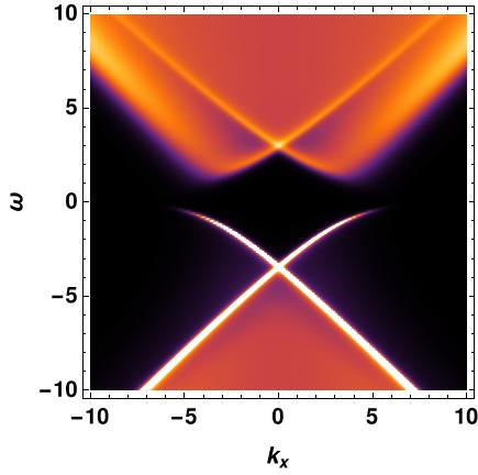
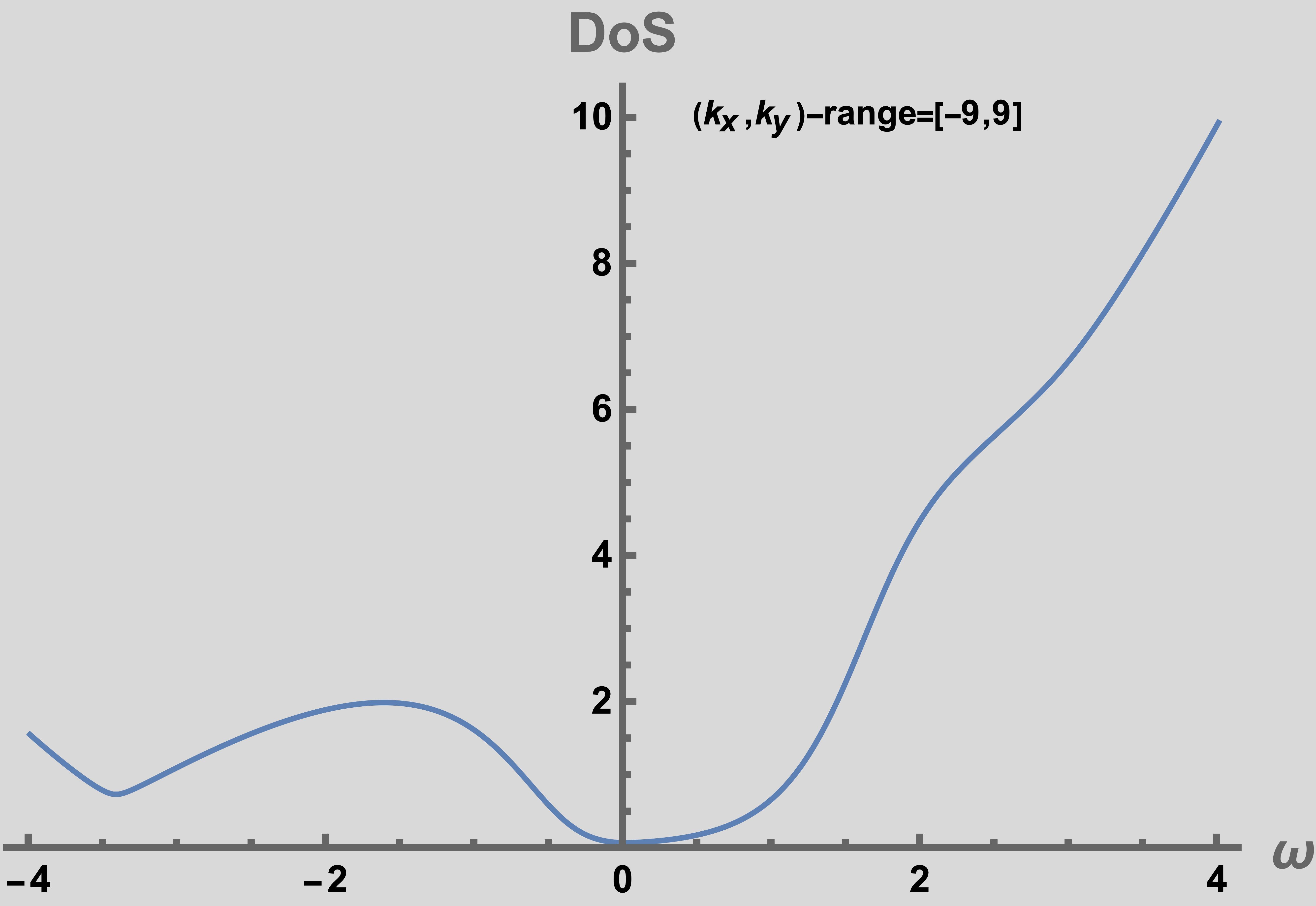
(a) $F_{\mu\nu}\Gamma^{\mu\nu}$ at $T=0,q_{f}=1$

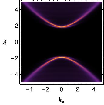
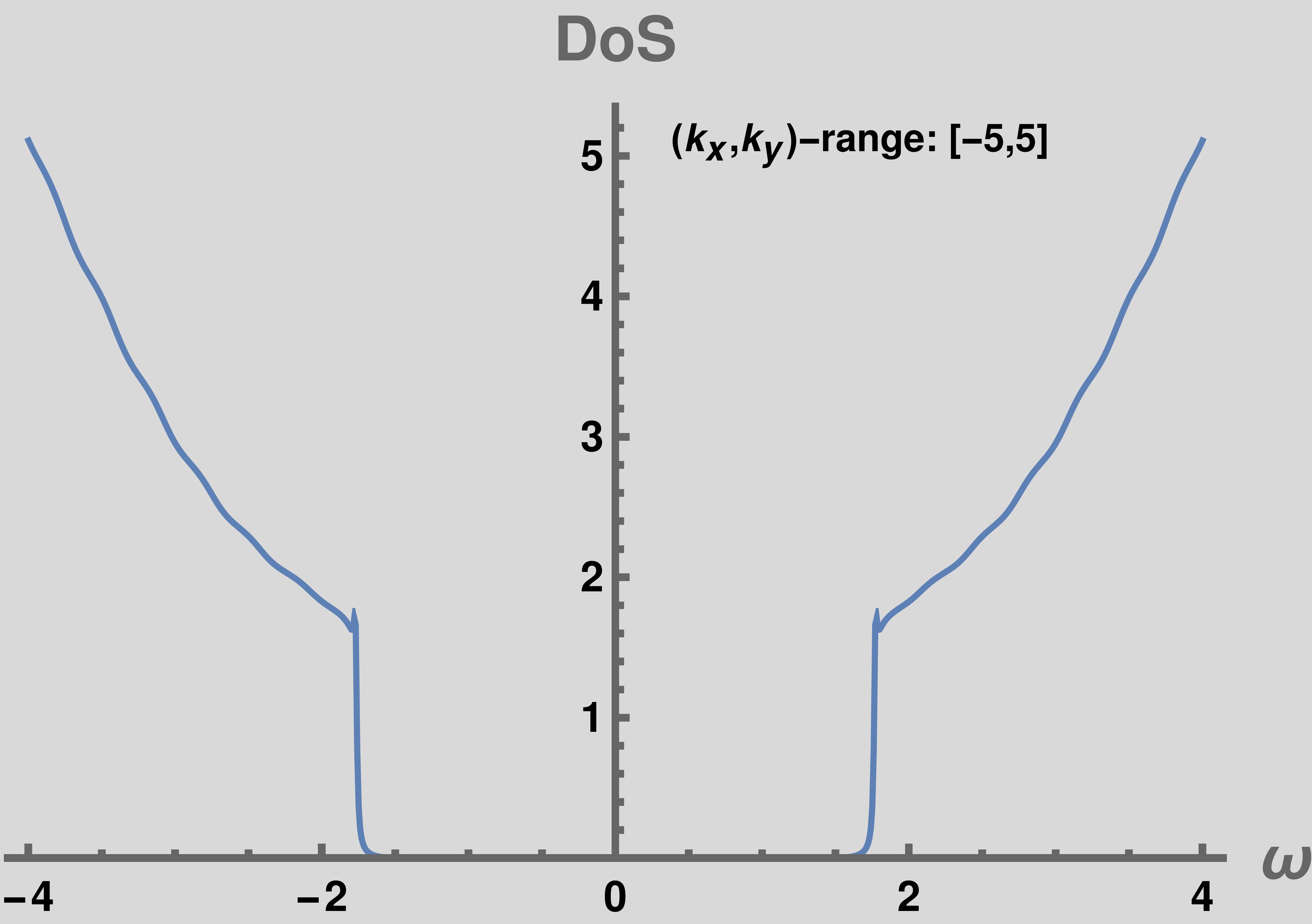
(b) $F^{2}$ at $T=0.025\mu,q_{f}=0$

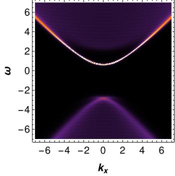
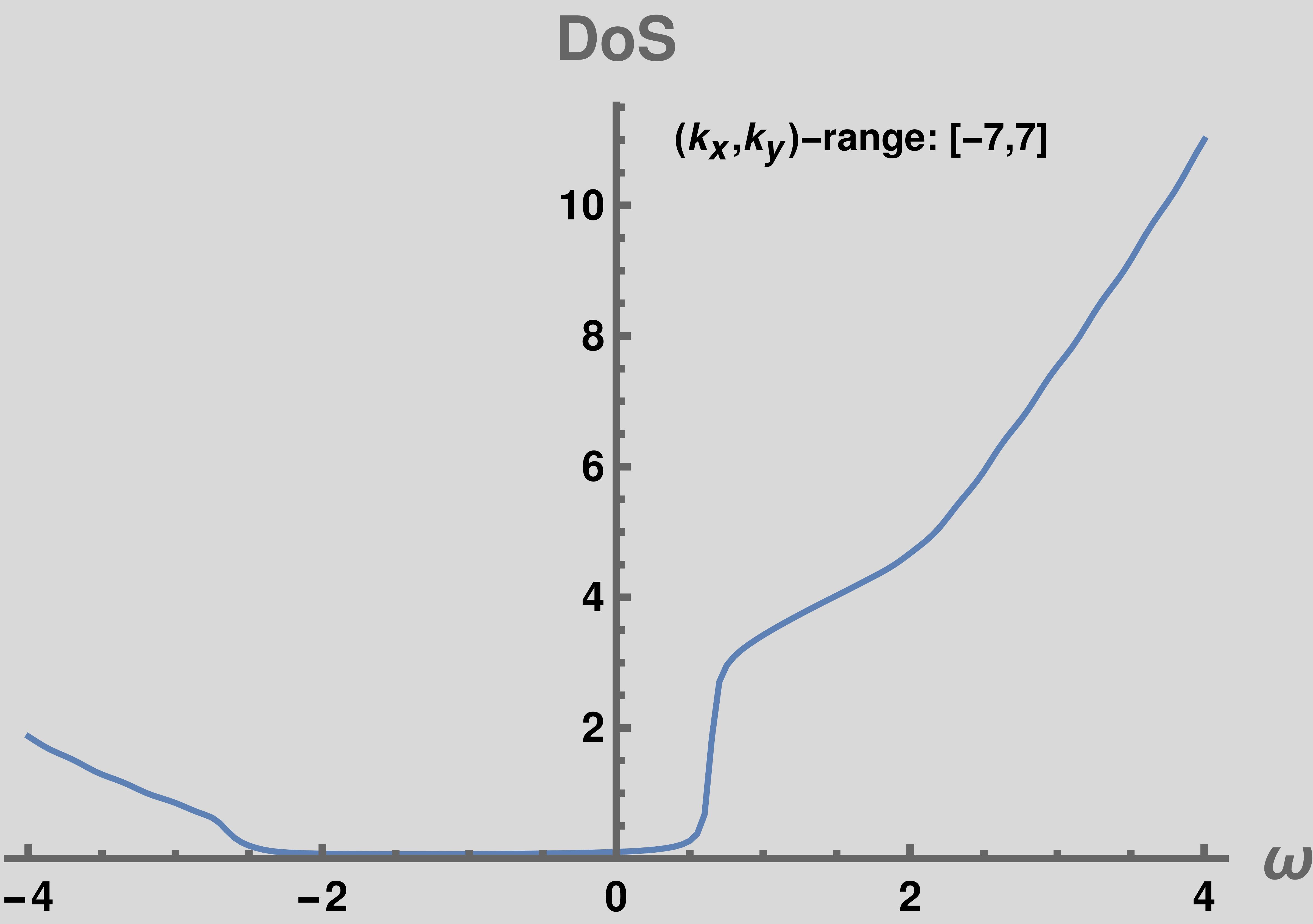
(c) $F^{2}$ at $T=0.025\mu,q_{f}=1$

Figure 1: Spectral function and density of state: (a) For dipole interaction at zero temperature, Mott gap is soft and asymmetric. (b) For density interaction ($\eta F^{2}\bar{\psi}\psi$) with $q_{f}=0$, Mott gap is hard and symmetric. (c) With minimal interaction included also, the Mott gap is hard and asymmetric due to the shifted Fermi surface.

We now explore all possible interactions that can generate a gap without any symmetry breaking. As we mentioned earlier, we have also examined other three possible cases $\Gamma^{scalar}=i\Gamma^{5},\Gamma^{z},i\Gamma^{5z}$. From the spectral function and DoS, we have found that $F^{2}\bar{\psi}i\Gamma^{5}\psi$ generates Mott gap while the other two interactions do not show any gap feature in the spectral function (table 1). One noticing point is that the gap size for the $F^{2}\bar{\psi}\psi$ interaction is larger than the gap size for the $F^{2}\bar{\psi}i\Gamma^{5}\psi$ interaction. The comparison of the DoS with the same parameter values for different interactions at $T=0.025\mu$ is shown in figure 2. This is clear evidence that $F^{2}\bar{\psi}\psi$ interaction is more suitable for describing the Mott gap in holography. The holographic flatband can also be realized using non-minimal gauge coupling with fermion ($F_{\mu\nu}\Gamma^{\mu\nu}\Gamma^{5}$). The fermion’s finite charge bends and shifts the flatband.

Gauge	$-i\eta\bar{\psi}L_{int}\psi$
Field	Gapless	Gap	Flatband	Effect of $q_{f}$
$A_{t}(z)dt$	$\Gamma^{z}F^{2}$, $i\Gamma^{5z}F^{2}$	$F^{2}(\eta>0),iF^{2}\Gamma^{5}$, $-iF_{\mu\nu}\Gamma^{\mu\nu}$	$F_{\mu\nu}\Gamma^{\mu\nu}\Gamma^{5}$	Shifting & Bending

Table 1: Mott gaps from different gauge field interactions

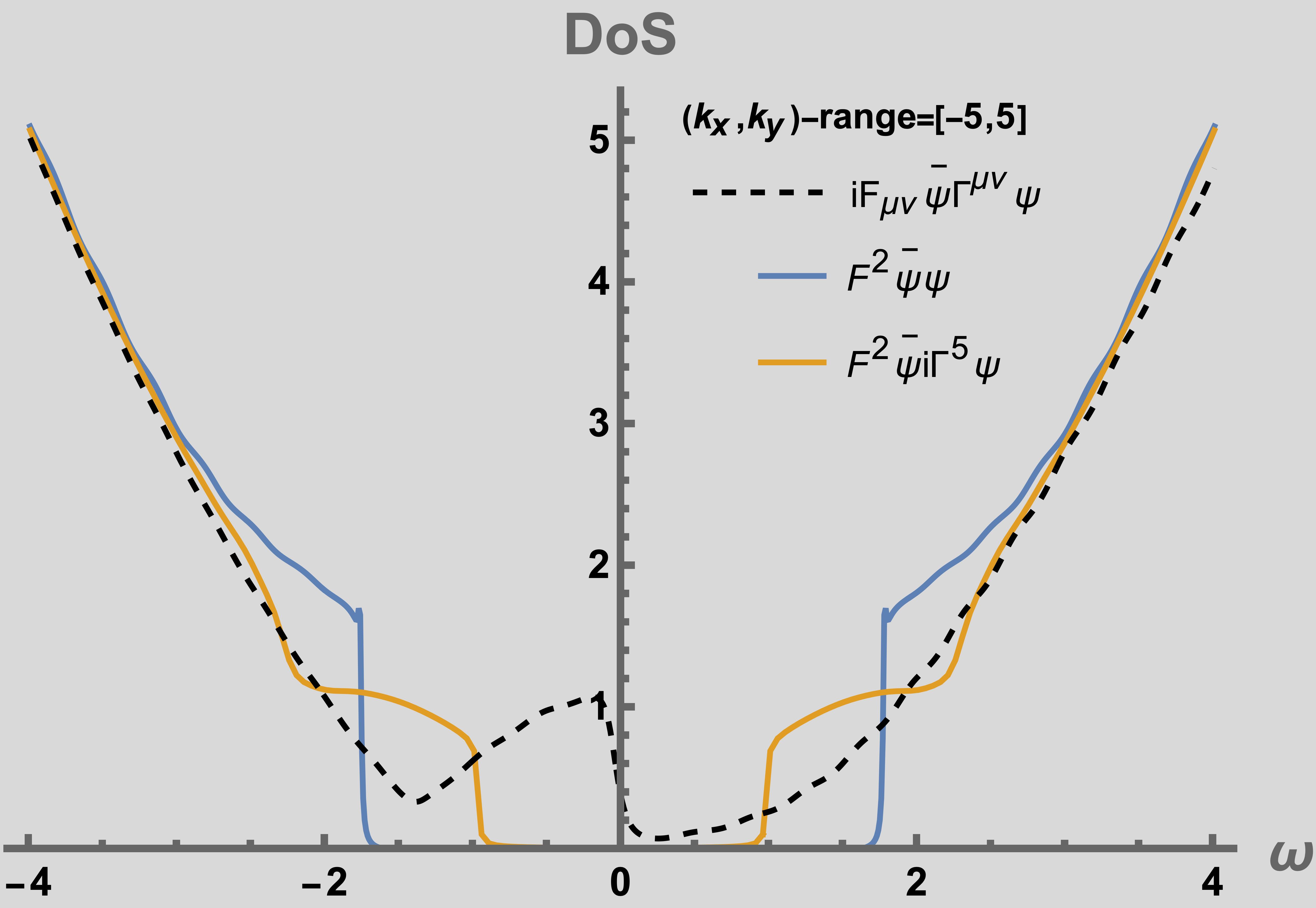
Figure 2: DoS for Mott gaps with different interactions at the same paratemeters.

We would like to investigate the effect of temperature, coupling strength, fermion mass in the spectral function as well as in the density of state. We know that the effect of the charge is to shift the position of the Fermi surface. In the presence of the charge $q_{f}=1$, we have also found the same feature here (figure 1(c)). The gap size $\Delta_{M}$ is measured from the DoS, where DoS$\leq 0.001$ region is considered as the gap region. It depends on the chemical potential and the temperature. Since the Mott gap is generated due to non-minimal gauge field interaction, the gap size is proportional to the chemical potential. The effect of the coupling strength on the gap size is shown in figure 3(a). The dependency of gap size on the temperature (figure 3(b)) shows a phase transition from Mott insulator to metal transition. The gap size decreases as the bulk fermion mass increases from zero to $\frac{1}{2}$. The nature of the spectral function changes to pole type when $m_{f}=\frac{1}{2}$ which is consistent with the previous investigation zaanen2015holographic . Since gap generation is due to interacting term, and $m_{f}=\frac{1}{2}$ in holography leads to non-interacting theory, the gap tends to vanish as $m_{f}=\frac{1}{2}$. However, we observe that there is a finite gap size at $m_{f}=\frac{1}{2}$ when coupling strength is turned on. We have shown the effect of coupling strength, fermion mass and temperature on the gap size in figure 3.

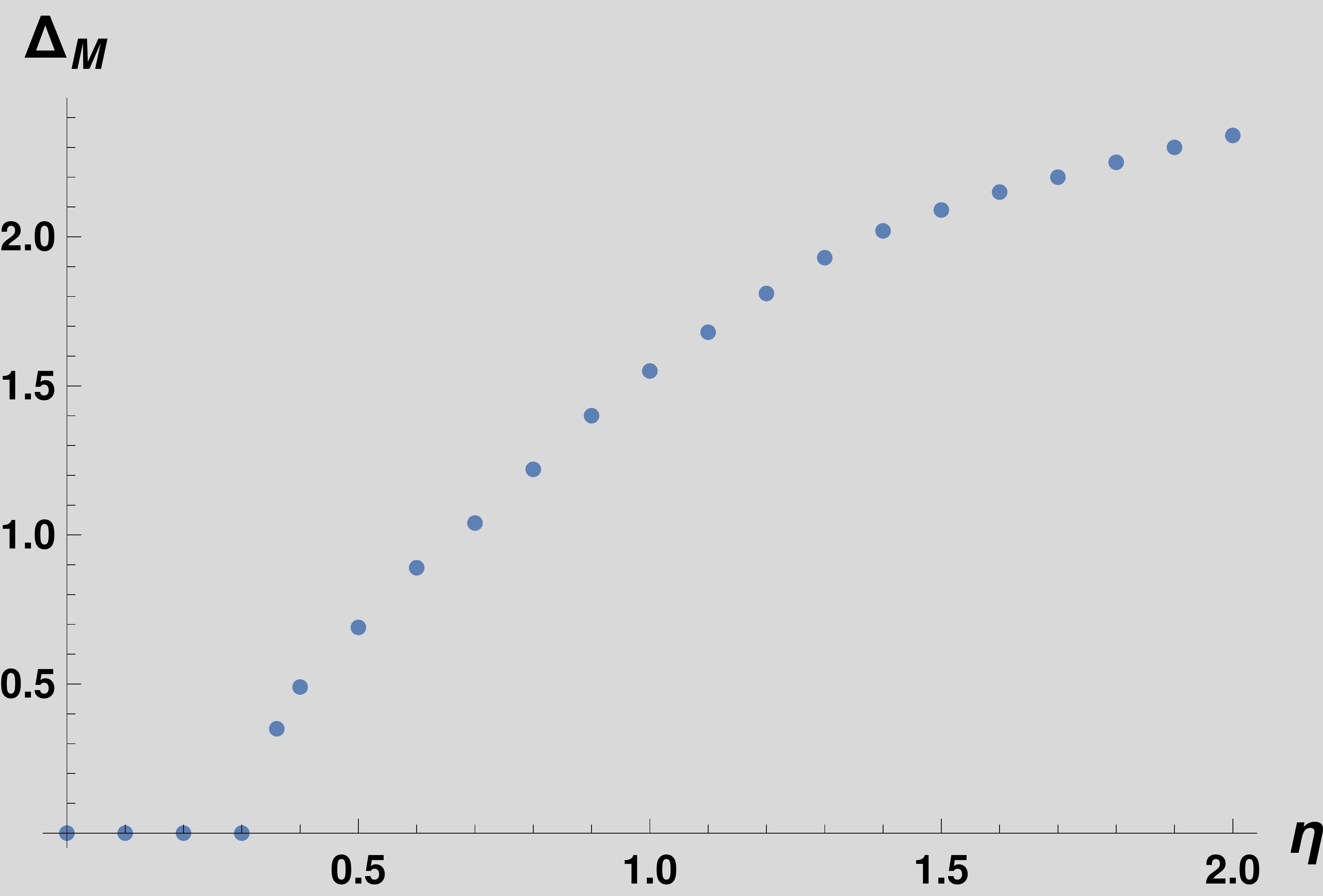
(a) Gap vs Coupling

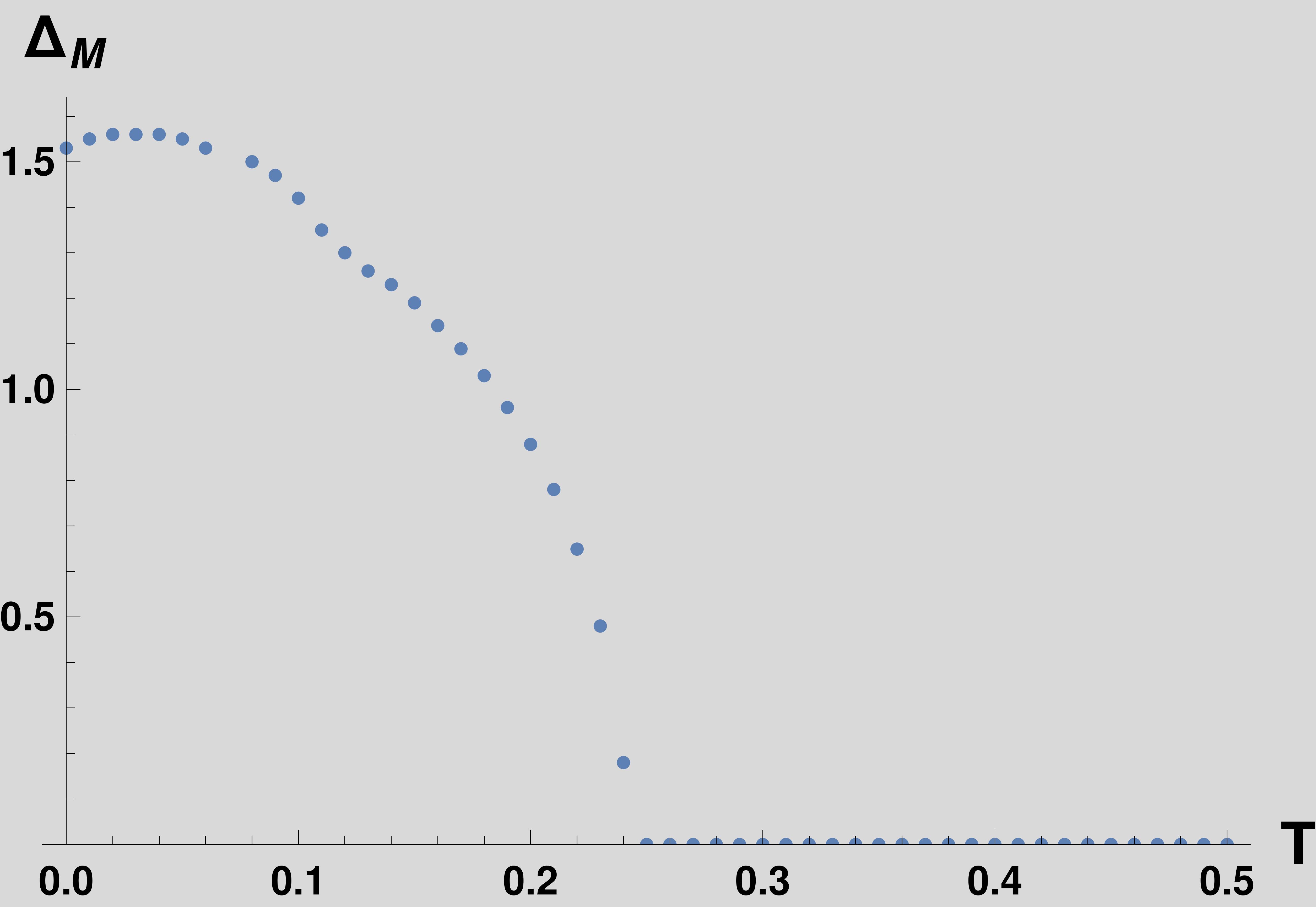
(b) Gap vs Temperature

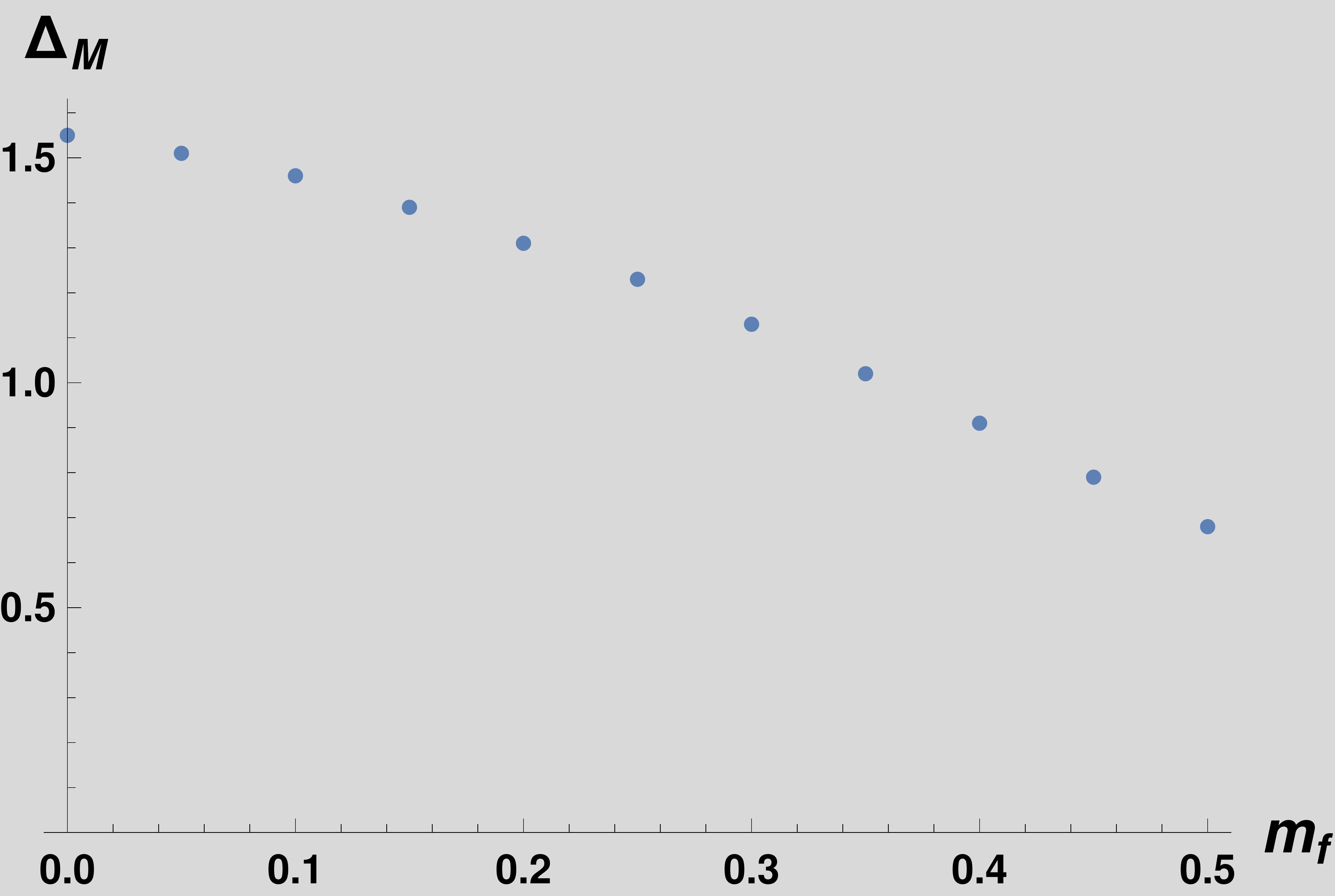
(c) Gap vs Fermion mass

Figure 3: Mott gap size $\Delta_{M}$ from DoS where DoS$\leq 0.001$ value is considered as cutoff for gap. (a) At $T=0.025\mu,m_{f}=0$ (b) For $\mu=2,\eta=1,m_{f}=0$, (c) For $T=0.025\mu,\eta=1$.

4 Classification of gaps in two flavor fermions

In this section, we promote our flavor analysis to two flavor fermions related to sublattice symmetry in materials. We will examine whether the dipole interaction can create a symmetric Mott gap. Besides this, we will also investigate $F^{2}\bar{\psi}_{1}\Gamma^{scalar}\psi_{2}$ interaction. In the two-flavor fermions setup, the Lagrangian density becomes

$$\mathcal{L}=\sum_{j=1}^{2}i\bar{\psi}_{j}\left(\Gamma^{\mu}D_{\mu}-m_{f}\right)\psi_{j}-i\bar{\psi_{1}}L_{int}\psi_{2}-i\bar{\psi_{2}}L_{int}\psi_{1}~{}~{}.$$ (15)

The corresponding coupled equation of motion of two flavor fermions read

$$\left(\Gamma^{\mu}D_{\mu}-m_{f}\right)\psi_{1}-L_{int}\psi_{2}=0,~{}~{}~{}\text{and}~{}~{}~{}\left(\Gamma^{\mu}D_{\mu}-m_{f}\right)\psi_{2}-L_{int}\psi_{1}=0~{}.$$ (16)

The procedure of Green’s function derivation for two flavor fermion is almost the same with one flavor case, which is given in detail in Oh:2020cym ; Sukrakarn:2023ncp . In the two flavor scenario, we mainly focus on the standard-standard (SS) and standard-alternative (SA) quantization. One noticeable point is that $G^{\text{SS}}=\Gamma^{5}G^{\text{SA}}$ relates SS and SA quantizations in terms of the output of the spectral function. The spectral function for two flavor case for $L_{int}=i\eta F^{2}\Gamma^{5}$ with SS quantization is shown in figure 4. The effect of the charge and the fermion mass on the spectral function is shown in figure 4 and 5 respectively. The role of bulk fermion mass is to determine the singularity structure of the Green’s function zaanen2015holographic . It changes branch-type singularity to pole type singularity when $m_{f}\rightarrow\frac{1}{2}$. Unlike one flavor case, the Mott gap in two flavors almost vanishes when $m_{f}=\frac{1}{2}$, which is shown in the spectral function plot (see figure 5). Although the interaction term is turned on, the system tends to be non-interacting when $m_{f}=\frac{1}{2}$. In the two-flavor fermion with SS-quantization, the $L_{int}=i\eta F^{2}\Gamma^{5}$ interaction only shows the Mott gap feature in the spectral function. The dipole interaction term in two flavor fermion shows no gap feature. We have summarized all non-minimal gauge field interactions in Table 2.

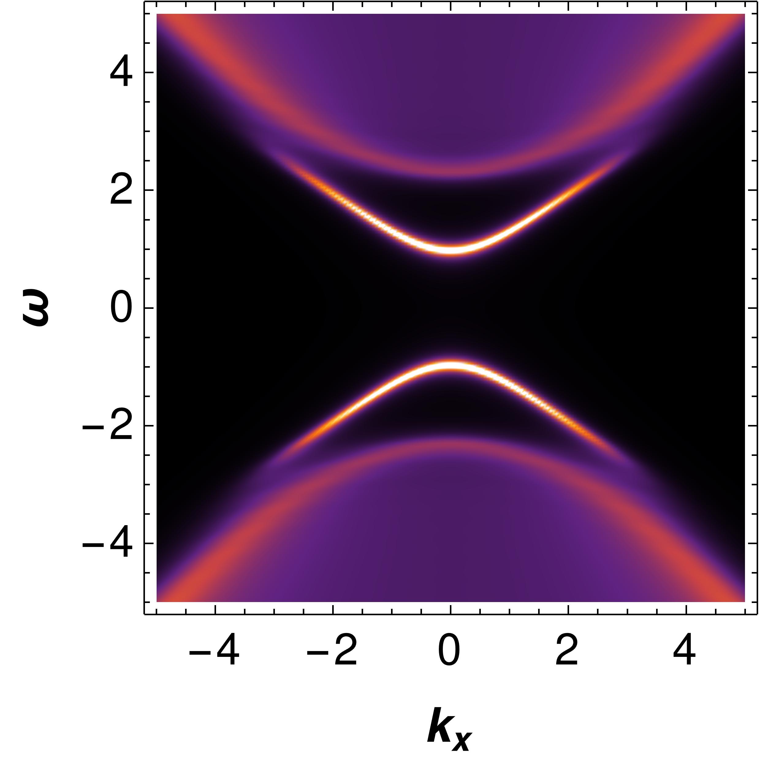
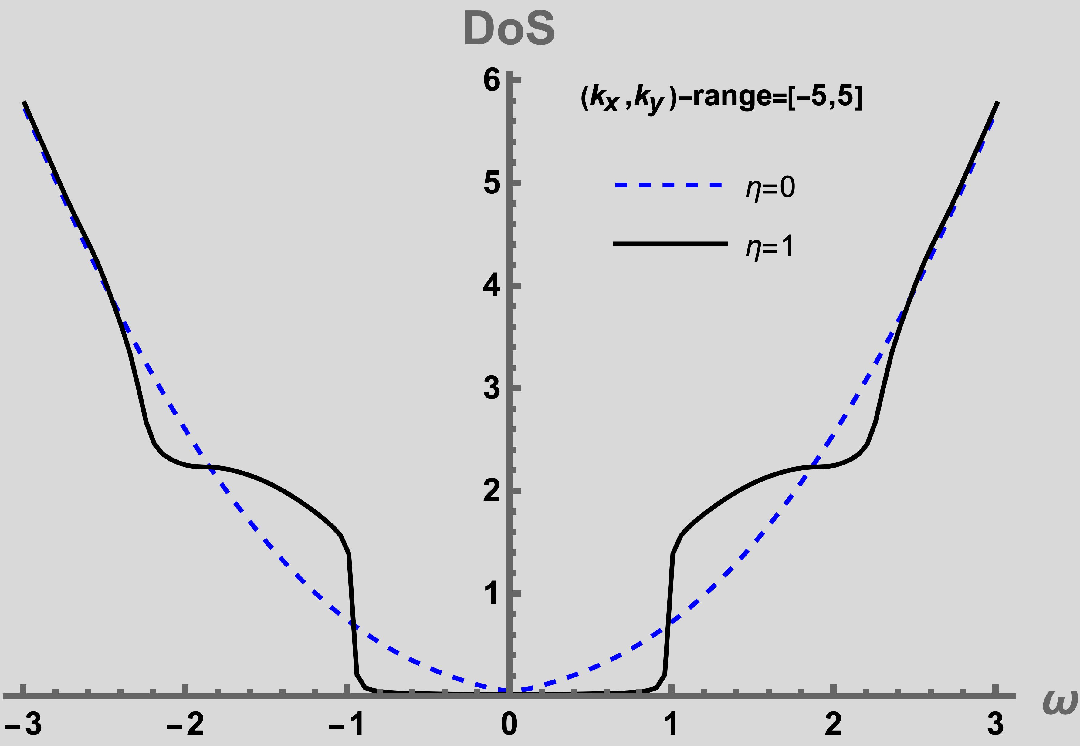
(a) For charge $q_{f}=0$

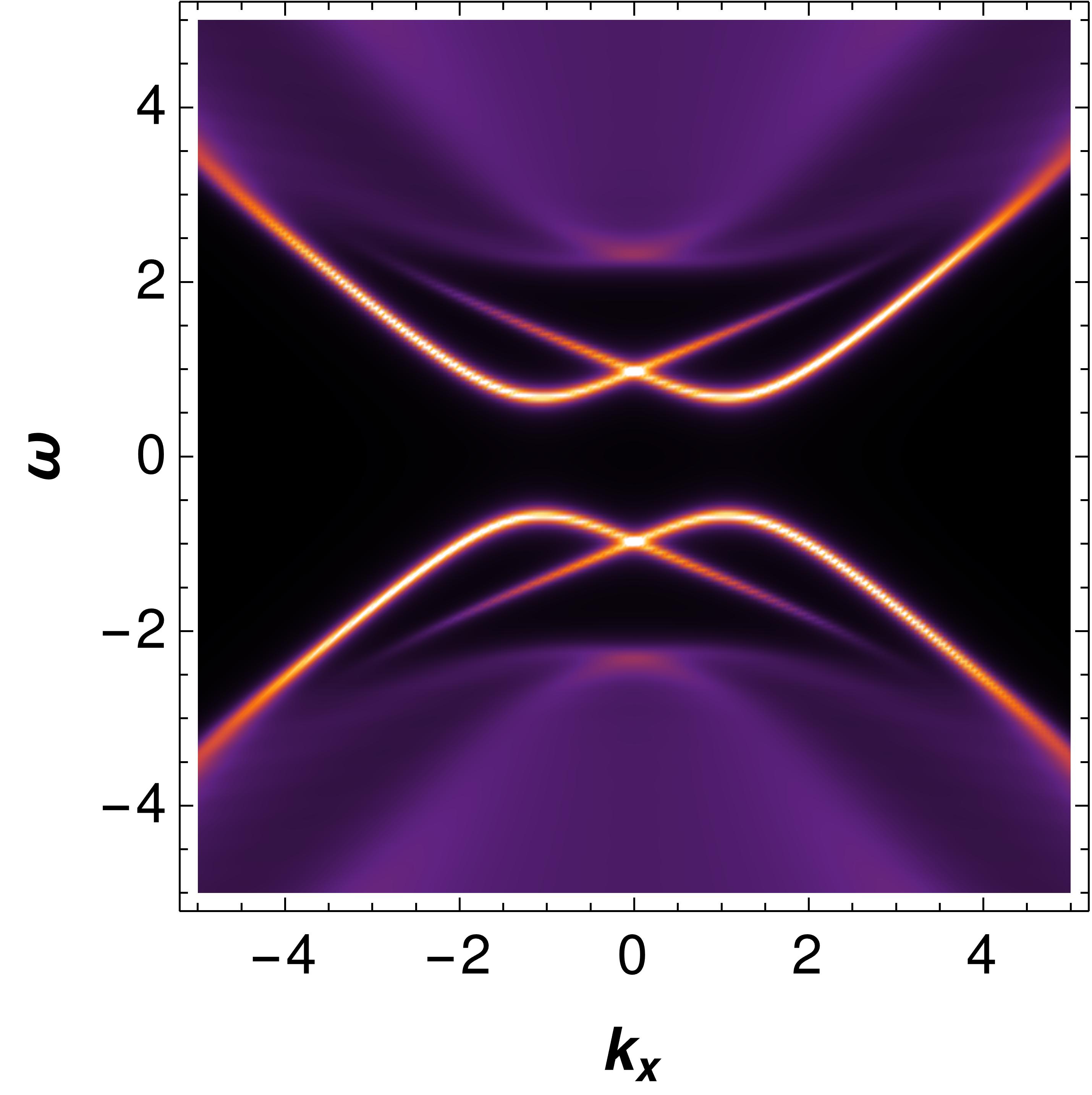
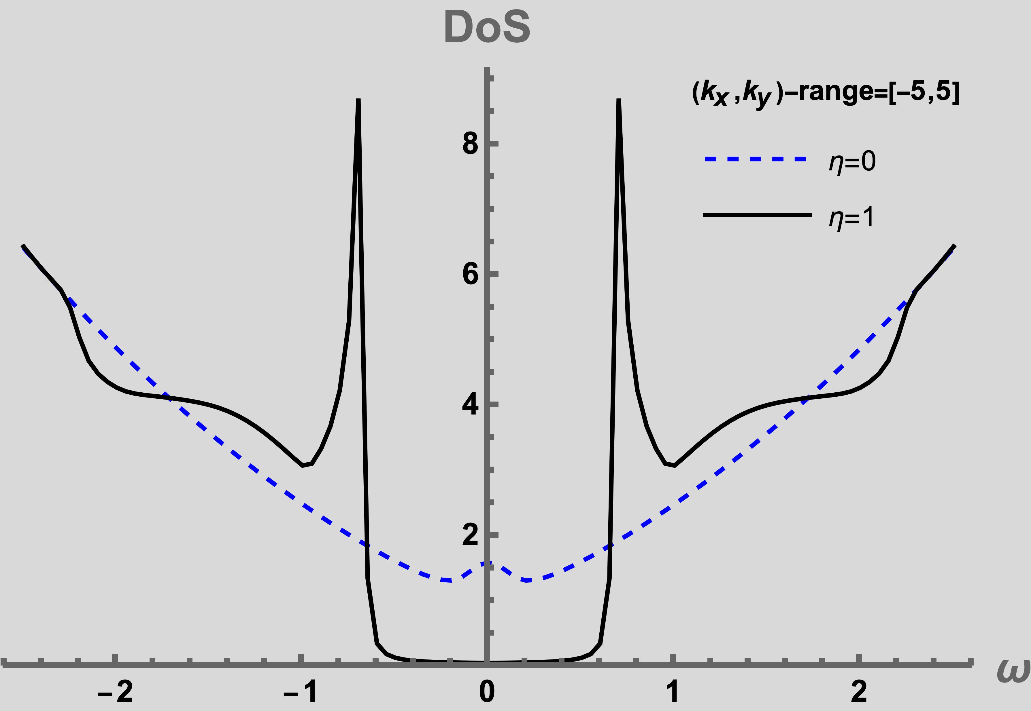
(b) For charge $q_{f}=1$

Figure 4: Spectral function along with DoS for $L_{int}=i\eta F^{2}\Gamma^{5}$ at $T=0.025\mu$.

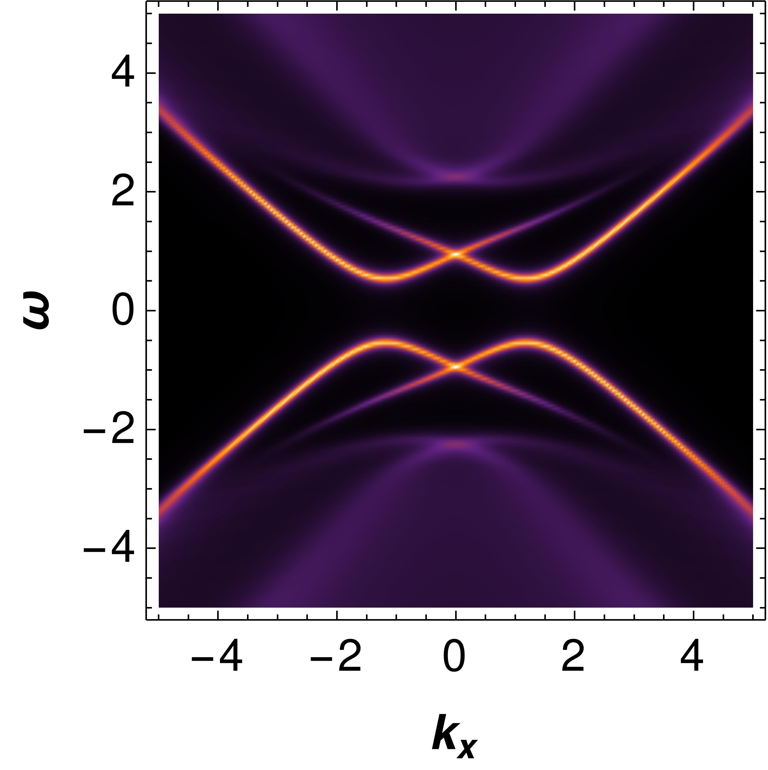
(a) For $m_{f}=0.1$

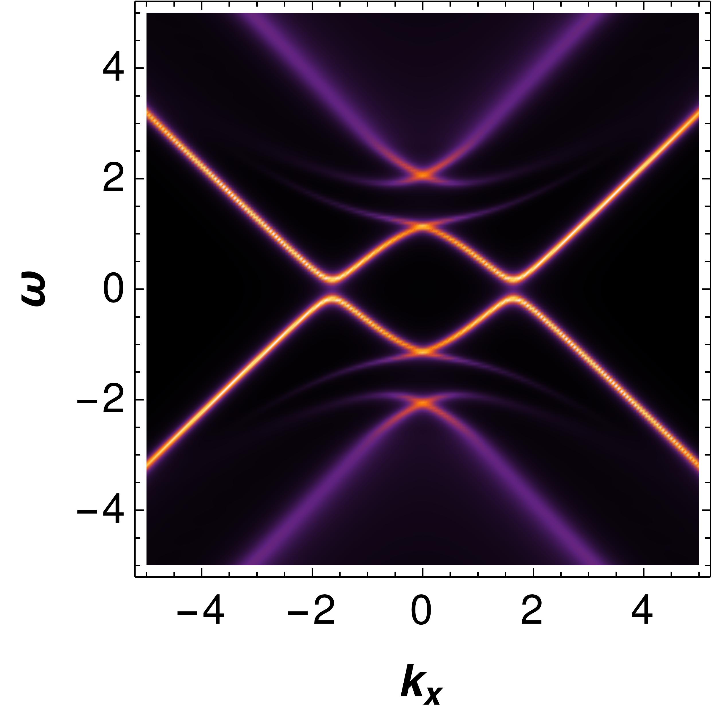
(b) For $m_{f}=0.4$

(c) For $m_{f}=0.5$

Figure 5: Effect of the fermion mass on SF at $T=0.025\mu$.

Gauge	$-i\bar{\psi}_{1}L_{int}\psi_{2}$ with SS-quantization, $SS=\Gamma^{5}SA$
$A=A_{t}(z)dt$	Gapless	Gap	Flatband	Effect of $q$
$F^{2}$-term	$\eta F^{2}$, $i\eta F^{2}\Gamma^{z}$	$i\eta F^{2}\Gamma^{5}$		Shifting FS
Dipole-term	$i\eta F_{\mu\nu}\Gamma^{\mu\nu}$, $\eta F_{\mu\nu}\Gamma^{\mu\nu}\Gamma^{z}$		$\eta F_{\mu\nu}\Gamma^{\mu\nu}\Gamma^{5}$	Shifting & Bending

Table 2: Mott gaps and flatband from non-minimal interactions for two flavor fermions.

For completeness, we now focus on the ordered gap generated by the symmetric breaking. The superconducting gap is classified as an ordered gap. There are three ordered gap types: $s$-, $p$- and $d$-wave ordered gap. In holographic models, these three ordered gaps have been realized from charged scalar Hartnoll:2008vx ; Hartnoll:2008kx ; Horo2009 ; Horowitz:2009ij ; ghorai2016higher ; Ghorai:2016tvk ; Ghorai:2021uby , vector Gubser:2008wv ; Vegh:2010fc ; Ghorai:2022gzx , and symmetric tensor Benini_2010 ; Chen:2010mk ; Zeng:2010fx ; Gao:2011aa ; Krikun:2013iha ; Nishida:2014lta ; Krikun:2015tga fields. The action for holographic superconductors (bosonic sector) are given as follows:

$$S_{b}=\int d^{4}x\frac{\sqrt{-g}}{2\kappa^{2}}\left[R+\frac{6}{L^{2}}+2\kappa^{2}\left(-\frac{1}{4}F_{\mu\nu}F^{\mu\nu}+\mathcal{L}_{matter}\right)\right]$$ (17)

where $\mathcal{L}_{matter}$ for scalar, vector and tensor fields are given in Yuk:2022lof , Ghorai:2023wpu and Ghorai:2023vuo respectively. In these references, the spectral function analysis for $s,p,d$-wave superconductors has also been done in detail, which is summarized in table 3. We set $\kappa=1,L=1,q=2$. Given the value of $\frac{T}{\mu}$, we can solve numerically all coupled bosonic field equations. In the presence of these bosonic fields, we observe different ordered gaps in the fermionic spectral function for the scalar field, vector field, and symmetric tensor field. To incorporate the particle-hole symmetry, we have to consider Nambu-Gorkov (NG) representation Yuk:2022lof , where conjugate $\psi_{c}=\psi^{*}$ is considered as independent degree of freedom.

Ordered	$\eta\bar{\psi}L_{int}\psi_{c}$ with Nambu-Gorkov spinor Ghorai:2023wpu
Gap	Sc. Gap	Flatband
$s$-wave	$\phi i\Gamma^{z}$
$p$-wave	$V_{\mu}\Gamma^{\mu},V_{\mu}i\Gamma^{5}\Gamma^{\mu}(R),V_{\mu\nu}\Gamma^{\mu\nu}$	$V_{\mu}\Gamma^{\mu}\Gamma^{z}$ (1-dim.)
$d$-wave	$B_{\mu\nu}\Gamma^{\mu}D^{\nu}$

Table 3: The ordered gap: $\phi$ is scalar field, $V_{\mu}$ is vector field and $B_{\mu\nu}$ is symmetric tensor field. $V_{\mu\nu}$ is the covariant derivative of the vector field and $R$ presents the rotation of Fermi arc. The spatial component of vector field and symmetric tensor field show $p$-wave and $d$-wave superconductivity respectively.

Here, we compare the order gap and the Mott gap from the density of states. With the same parameters at $T=0.025\mu$, the Mott gap size is larger than superconducting gap, as shown in figure 6. Given the values of $T$ and $\mu$, the Mott gap is generated directly through the gauge coupling, whereas the superconducting gap in fermion spectral function is triggered by the condensation value, which is generated by the spontaneous symmetry breaking. The dependency of parameters for Mott gaps and superconducting gaps show the same behavior. However, the mechanisms of these two gap generations are completely different. The superconducting gap in a fermionic spectral function is associated with $U(1)$-symmetry breaking and minimal coupling between the fermion and the order parameter, whereas the Mott gaps are associated with non-minimal coupling of the gauge field and fermion. In the NG representation, the one dimensional flatband is also realized from a spatial vector field interaction with fermion ($V_{\mu}\Gamma^{\mu}\Gamma^{z}$), which shown in table 3.

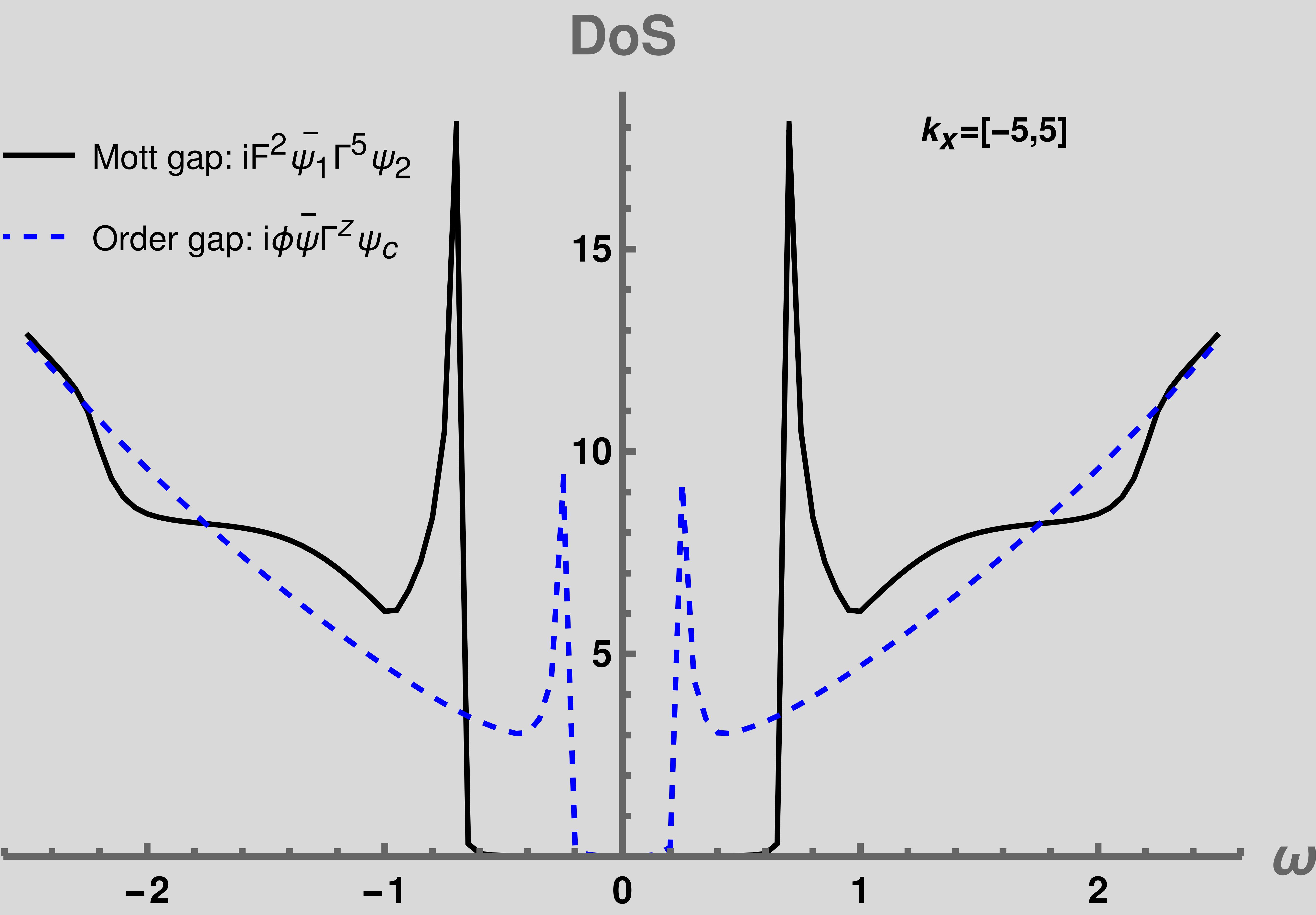
Figure 6: Compare of DoS for Mott gap and order gap at $T=0.025\mu$ with same $\eta$.

5 Summary

In this paper, we have addressed the analysis of the density of states for Mott gaps and superconducting gaps in holographic setups. Without manifest symmetry breaking, the gap generation is known as the Mott gap, whereas the superconducting gap is generated because of symmetry breaking. Using gauge/gravity duality, these two gaps are explained in the literature, where Mott physics is elucidated using dipole interaction PhysRevLett.106.091602 . It is a non-minimal gauge coupling with fermions that generates a gap in the fermionic spectral function without a symmetry-breaking mechanism. In the previous investigation PhysRevLett.106.091602 , the Mott gap in the spectral function is asymmetric, and one of the bands seems to touch the Fermi level at $\omega=0$. To gain a clearer view of the Mott gap size, we have calculated the density of states (DoS), which shows a soft and asymmetric Mott gap, whereas DMFT results show differently. This motivates us to consider other non-minimal gauge couplings with fermions. First, we have considered an density-density coupling ($F^{2}\bar{\psi}\psi$) term, which can be mapped to the interaction part of the Hubbard Hamiltonian. This mapping also justifies our proposal. Then, we have calculated the spectral function along with the DoS, which clearly shows a strong and symmetric Mott gap feature. Other possible non-minimal gauge field interactions (26) have been examined, and the Mott gap size in the DoS (figure 2) has been compared. The DoS figure also supports our claim about the proper Mott gap in the fermionic spectral. We have classified Mott gaps, namely, soft gap and hard gap. For the dipole interaction case, we can treat the Mott gap as a soft and asymmetric gap, whereas the $F^{2}$ interactions produce a hard and symmetric Mott gap.
The effects of the fermion charge, coupling strength, temperature, and fermion mass are important for further investigation. To observe the effects of these parameters on the Mott gaps, we measured the gap size $\Delta_{M}$ from the DoS, where DoS$\leq 0.001$ region is a gapped region. The gap size is plotted in figure 3. We observed that the Mott gap is vanishing at $T=0.13\mu$. Therefore, this can be treated as the critical temperature for the Mott insulator-metal transition. Finite fermion mass decreases the Mott gap size. In the limit of the fermion mass $m_{f}=\frac{1}{2}$, we found that the structure of singularity type changes from a branch-cut type to a simple pole structure, which matches with previous findings zaanen2015holographic . We also have found that the dipole interaction term with $\Gamma^{5}$ shows a flatband in the spectral function. This is the non-minimal gauge interaction which creates a flatband in a holographic setup.
Next, we have classified interactions in terms of Mott and superconducting gaps. To achieve this, we first examined all non-minimal gauge field interactions in two-flavor fermions. We found that in two-flavor fermions, only the density interaction ($F^{2}i\Gamma^{5}$) creates a Mott gap, while the dipole term doesn’t produce any gap feature in the spectral function. For the fermion mass $m_{f}=\frac{1}{2}$, the system nearly becomes non-interacting, despite the interaction strength being high $(\eta=1)$, which is not seen in the one-flavor fermion case. We have replicated three types of order gaps, which are summarized in table 3. When comparing the gap size in DoS for the same parameters, we observe that the Mott gap size is larger than the superconducting gap which is consistent with literature. Our future direction is to study the Fermi-Dirac distribution function from the holographic fermion.

Appendix A Mott Physics

Hubbard Hamiltonian (HH) is given by

$$H=-\sum_{<ij>,\sigma}t_{ij}c^{\dagger}_{i\sigma}c_{j\sigma}+H_{I}~{}.$$ (18)

where interaction Hamiltonian $H_{I}=U\sum_{i}n_{i\uparrow}n_{i\downarrow}$ with the fermionic number operator $n_{i\uparrow}=c^{\dagger}_{i\uparrow}c_{i\uparrow}$. In the Mean field approximation, we can write

$$n_{i\uparrow}n_{i\downarrow} \approx n_{i\uparrow}\langle n_{i\downarrow}\rangle+n_{i\downarrow}\langle n_{i\uparrow}\rangle-\langle n_{i\uparrow}\rangle\langle n_{i\downarrow}\rangle$$ (19)

which gives the interaction term in the HH as follows:

$$H_{I}=U\sum_{i}\left[n_{i\uparrow}\langle n_{i\downarrow}\rangle+n_{i\downarrow}\langle n_{i\uparrow}\rangle-\langle n_{i\uparrow}\rangle\langle n_{i\downarrow}\rangle\right]~{}.$$ (20)

The interpretation of this expression is that the up-spin fermions interact with the average density of the down-spin fermions, and similarly the down-spin fermions interact with the average density of the up-spin fermions. This HH governs Mott metal-insulator transition. We need to find a similar kind of interaction term in the holographic setup. The number density can be expressed in terms of charge density ($\rho$) which maps to the gauge field in the bulk theory. First, we need to assume that $\langle n_{i\uparrow}\rangle=\langle n_{i\downarrow}\rangle\propto\rho$. Therefore, the interaction part now becomes

$$H_{I}\propto\rho U\sum_{i}\left[c^{\dagger}_{i\uparrow}c_{i\uparrow}+c^{\dagger}_{i\downarrow}c_{i\downarrow}\right]-U\rho^{2}$$ (21)

which translates in momentum space as

$$H_{I}\propto U\rho\sum_{k}\left[c^{\dagger}_{k\uparrow}c_{k\uparrow}+c^{\dagger}_{k\downarrow}c_{k\downarrow}\right]-U\rho^{2} \approx U\rho\left[c^{\dagger}_{+\uparrow}c_{+\uparrow}+c^{\dagger}_{+\downarrow}c_{+\downarrow}+c^{\dagger}_{-\uparrow}c_{-\uparrow}+c^{\dagger}_{-\downarrow}c_{-\downarrow}\right]-U\rho^{2}~{}~{}~{}~{}~{}~{}~{}~{}$$ (22)

The last term in the right hand side of the above equation gives the shifting of the energy. We need to find a interaction terms in the holographic setup, which can map to $\left[c^{\dagger}_{+\uparrow}c_{+\uparrow}+c^{\dagger}_{+\downarrow}c_{+\downarrow}+c^{\dagger}_{-\uparrow}c_{-\uparrow}+c^{\dagger}_{-\downarrow}c_{-\downarrow}\right]$. We can identify the bulk fermion field $\psi=(c_{+\uparrow},c_{+\downarrow},c_{-\uparrow},c_{-\downarrow})^{T}$ where we are embedding $H_{I}$ into a higher dimension. Now the fermionic annihilation $(c_{\pm\uparrow\downarrow})$ and creation $(c^{\dagger}_{\pm\uparrow\downarrow})$ operators are function of radial coordinate and momentum Yuk:2022lof . Therefore, the suitable non-minimal coupling term for gauge field is $F^{2}\psi^{\dagger}\psi$ which is the non-relativistic(NR) interaction. We can promot this NR interaction term to the relativistic bulk interaction term in the following way:

$$\mathcal{L}_{int}=-i\bar{\psi}\eta F^{2}\psi$$ (23)

where $\eta$ is the coupling strength and $F^{2}=F_{\mu\nu}F^{\mu\nu}$. Note that $i\Gamma^{\underline{t}}$ is the dressing factor for the promoting relativistic form from the NR interaction since the kinetic term of the Lagrangian also contains this dressing factor. Since potential term in a Lagrangian is opposite to the Hamiltonian, we need to consider the negative sign in the interaction Lagrangian. Therefore, the most suitable In general, we can consider the following interaction Lagrangian

$$\mathcal{L}_{int}=\left\{\begin{array}[]{ c l }-i\eta\bar{\psi}F^{2}\Gamma^{scalar}\psi&\quad\textrm{Density type interaction}\\ -i\eta F_{\mu\nu}\bar{\psi}\Gamma^{\mu\nu}\Gamma^{scalar}\psi&\quad\textrm{Pauli interaction}\end{array}\right.~{}~{}.$$ (26)

where the possible gamma matrices are $\Gamma^{scalar}=\mathbb{I}_{4},\Gamma^{z},i\Gamma^{5},i\Gamma^{5z}$ although other interaction terms with different $\Gamma^{scalar}$ are not proportional to $\left[c^{\dagger}_{+\uparrow}c_{+\uparrow}+c^{\dagger}_{+\downarrow}c_{+\downarrow}+c^{\dagger}_{-\uparrow}c_{-\uparrow}+c^{\dagger}_{-\downarrow}c_{-\downarrow}\right]$. For the Pauli interaction $(\Gamma^{scalar}=\mathbb{I}_{4})$ in the non-relativistic limit, the interaction term $F_{\mu\nu}\bar{\psi}\Gamma^{\mu\nu}\psi$ becomes $\psi^{\dagger}F_{\mu\nu}\Gamma^{\mu\nu}\psi$. For the gauge field ansatz $A=A_{t}(z)dt$, the dipole interaction term can be expressed as

$$\mathcal{L}_{int}^{dipole}\propto\psi^{\dagger}F_{zt}\Gamma^{zt}\psi=z^{2}(\partial_{z}A_{t})\left[c^{\dagger}_{+\uparrow}c_{-\downarrow}-c^{\dagger}_{+\downarrow}c_{-\uparrow}-c^{\dagger}_{-\uparrow}c_{+\downarrow}+c^{\dagger}_{-\downarrow}c_{+\uparrow}\right]~{}.$$ (27)

The above expression can not be mapped to $\left[c^{\dagger}_{+\uparrow}c_{+\uparrow}+c^{\dagger}_{+\downarrow}c_{+\downarrow}+c^{\dagger}_{-\uparrow}c_{-\uparrow}+c^{\dagger}_{-\downarrow}c_{-\downarrow}\right]$ term. Therefore, we can argue that the reasonable interaction for Mott gap is the density type interaction (23). Since some interactions in eq.(26) produce gap feature in the spectral function, we will examine all possible interactios to find Mott gap feature in the DoS.

Appendix B Derivation of Green’s function

Rearranging all components of equations, we can recast the Dirac equations in the following structure

$$\partial_{z}\Psi_{+}+\mathbb{M}_{1}\Psi_{+}+\mathbb{M}_{2}\Psi_{-} = 0~{},$$ (28)

$$\partial_{z}\Psi_{-}+\mathbb{M}_{3}\Psi_{-}+\mathbb{M}_{4}\Psi_{+} = 0$$ (29)

where $2\times 2$-matrix $\mathbb{M}_{i},~{}i=1,2,3,4$ are given by

$$\mathbb{M}_{1}= \ -\frac{m_{f}+\eta F^{2}}{z\sqrt{f}}\mathbb{I}_{2},$$

$$\mathbb{M}_{2}= \ \frac{i}{\sqrt{f}}\begin{pmatrix}k_{y}&-\frac{(\omega+q_{f}A_{t})}{\sqrt{f}}+k_{x}\\ \frac{(\omega+q_{f}A_{t})}{\sqrt{f}}+k_{x}&-k_{y}\end{pmatrix}~{},$$

$$\mathbb{M}_{3}= \ -\mathbb{M}_{1},\quad\mathbb{M}_{4}=-\mathbb{M}_{2}~{}.~{}~{}~{}$$ (30)

There are two independent solutions since $\Psi_{+}$ and $\Psi_{-}$ are two components spinor. The general solution can be written in a linear combination of two solutions as

$$\Psi_{+}=\sum_{i=1}^{2}c_{i}\Psi_{+}^{(i)}=\mathbb{S}(z)\mathbf{c},$$

$$\Psi_{-}=\sum_{i=1}^{2}c_{i}\Psi_{-}^{(i)}=\mathbb{C}(z)\mathbf{c}$$ (31)

The $2\times 2$-matrix $\mathbb{S}(z),\mathbb{C}(z)$ are constructed from the solution, where the constant column vector $\mathbf{c}$ is constructed from the two coefficients of the linear combination. Substituting above eq.(31) in eq.(s)(28, 29), we obtain

$$\partial_{z}\mathbb{S}(z)+\mathbb{M}_{1}\mathbb{S}(z)+\mathbb{M}_{2}\mathbb{C}(z) = 0~{},$$ (32)

$$\partial_{z}\mathbb{C}(z)+\mathbb{M}_{3}\mathbb{C}(z)+\mathbb{M}_{4}\mathbb{S}(z) = 0~{}.$$ (33)

The boundary solution tells us that we need to define $U(z)=diag(z^{m_{f}},z^{m_{f}})$ to get normalized boundary Green’s function. Then we can write the boundary solution from eq.(31)

$$\Psi_{+}(z)\overset{z\rightarrow 0}{\approx}U(z)\mathbb{S}_{0}\mathbf{c},~{}~{}~{}~{}\Psi_{-}\overset{z\rightarrow 0}{\approx}U(z)^{-1}\mathbb{C}_{0}\mathbf{c}~{},$$ (34)

where $\mathbb{S}_{0},\mathbb{C}_{0}$ are the $z$-independent boundary $2\times 2$-matrix. We can define

$$\mathcal{J}=\mathbb{S}_{0}\mathbf{c},~{}~{}~{}~{}~{}\mathcal{C}=\mathbb{C}_{0}\mathbf{c}$$ (35)

which translate the boundary solution (eq.(34)) as

$$\Psi_{+}\overset{z\rightarrow 0}{\approx}U(z)\mathcal{J},~{}~{}~{}~{}\Psi_{-}\overset{z\rightarrow 0}{\approx}U(z)^{-1}\mathcal{C}~{}.$$ (36)

Comparing eq.(36) with eq.(9), we find

$$\mathcal{J}=\mathbf{A},~{}~{}~{}~{}\mathcal{C}=\mathbf{D}$$ (37)

We can also get the relation between $\mathcal{C}$ and $\mathcal{J}$ from eq.(35)

$$\mathcal{C}=\mathbb{C}_{0}\mathbb{S}^{-1}_{0}\mathcal{J}~{}.$$ (38)

From the boundary action (eq.(10)), we can write

$$S_{bdy}=\int d^{3}x\mathcal{J}^{\dagger}\tilde{\Gamma}\mathcal{C}+h.c.$$ (39)

Using eq.(38), the boundary action now becomes

$$S_{bdy}=\int d^{3}x\mathcal{J}^{\dagger}\tilde{\Gamma}\mathbb{C}_{0}\mathbb{S}^{-1}_{0}\mathcal{J}+h.c.=\int d^{3}x\mathcal{J}^{\dagger}\mathbb{G}_{R}\mathcal{J}+h.c.~{}~{}~{}~{}~{}$$ (40)

where the retarded Green’s function $\mathbb{G}_{R}=\tilde{\Gamma}\mathbb{C}_{0}\mathbb{S}^{-1}_{0}$. We can promote this boundary Green’s function into bulk Green’s function by considering the $z$-dependent Green’s function as follows:

$$\mathbb{G}=\tilde{\Gamma}\mathbb{C}(z)\mathbb{S}^{-1}(z)$$ (41)

where $\mathbb{C}(z),\mathbb{S}(z)$ is defined in eq.(31). Taking the derivative of the above equation, we get

$$\partial_{z}\mathbb{G}(z)=\tilde{\Gamma}\left[\partial_{z}\mathbb{C}(z)\mathbb{S}^{-1}(z)-\mathbb{C}(z)\mathbb{S}^{-1}(z)(\partial_{z}\mathbb{S}(z))\mathbb{S}^{-1}(z)\right]~{}~{}~{}~{}~{}$$ (42)

Using eq.(s)(32,33), we have found

$$\partial_{z}\mathbb{G}(z)+\tilde{\Gamma}\mathbb{M}_{3}\tilde{\Gamma}\mathbb{G}(z)-\mathbb{G}(z)\mathbb{M}_{1}-\mathbb{G}(z)\mathbb{M}_{2}\tilde{\Gamma}\mathbb{G}(z)+\tilde{\Gamma}\mathbb{M}_{4}=0~{}~{}~{}~{}~{}$$ (43)

This is the desired flow equation to know the bulk Green’s function $\mathbb{G}(z)$. From eq.(34), we can express

$$\mathbb{S}(z)\overset{z\rightarrow 0}{\approx}U(z)\mathbb{S}_{0}~{}~{}\text{and}~{}~{}\mathbb{C}(z)\overset{z\rightarrow 0}{\approx}U(z)^{-1}\mathbb{C}_{0}~{}.$$ (44)

By substituting the above relations, we can now map the boundary Green’s function with bulk Green’s function near the boundary in the following way

$$\mathbb{G}(z)\overset{z\rightarrow 0}{\approx}U(z)^{-1}\mathbb{G}_{R}U(z)^{-1}$$ (45)

where we have used the fact $\tilde{\Gamma}U(z)^{-1}\tilde{\Gamma}=U(z)^{-1}$. To solve the flow equation, we need to know the horizon value of the Green’s function which is $\mathbb{G}(z_{h})=i\mathbb{I}_{2}$.

References

- (1) P. A. Lee, N. Nagaosa, and X.-G. Wen, Doping a mott insulator: Physics of high-temperature superconductivity, Rev. Mod. Phys. 78 (Jan, 2006) 17–85.
- (2) A. Georges, G. Kotliar, W. Krauth, and M. J. Rozenberg, Dynamical mean-field theory of strongly correlated fermion systems and the limit of infinite dimensions, Rev. Mod. Phys. 68 (Jan, 1996) 13–125.
- (3) P. W. Phillips, L. Yeo, and E. W. Huang, Exact theory for superconductivity in a doped mott insulator, Nature Physics 16 (2020) 1175–1180.
- (4) N. F. MOTT, Metal-insulator transition, Rev. Mod. Phys. 40 (Oct, 1968) 677–683.
- (5) J. M. Maldacena, The Large N limit of superconformal field theories and supergravity, Int.J.Theor.Phys. 38 (1999) 1113–1133, [hep-th/9711200].
- (6) S. S. Gubser, I. R. Klebanov, and A. M. Polyakov, Gauge theory correlators from noncritical string theory, Phys. Lett. B428 (1998) 105–114, [hep-th/9802109].
- (7) E. Witten, Anti-de Sitter space and holography, Adv. Theor. Math. Phys. 2 (1998) 253–291, [hep-th/9802150].
- (8) S. A. Hartnoll, P. K. Kovtun, and M. S. Müller, Theory of the Nernst effect near quantum phase transitions in condensed matter and in dyonic black holes, Phys. Rev. B 76 (Oct., 2007) 144502, [arXiv:0706.3215].
- (9) Y. Seo, G. Song, P. Kim, S. Sachdev, and S.-J. Sin, Holography of the Dirac Fluid in Graphene with two currents, Phys. Rev. Lett. 118 (2017) 036601, [arXiv:1609.03582].
- (10) E. Oh, T. Yuk, and S.-J. Sin, The emergence of strange metal and topological liquid near quantum critical point in a solvable model, JHEP 11 (2021) 207, [arXiv:2103.08166].
- (11) G. Song, J. Rong, and S.-J. Sin, Stability of topology in interacting Weyl semi-metal and topological dipole in holography, JHEP 10 (2019) 109, [arXiv:1904.09349].
- (12) E. Oh, Y. Seo, T. Yuk, and S.-J. Sin, Ginzberg-Landau-Wilson theory for Flat band, Fermi-arc and surface states of strongly correlated systems, arXiv:2007.12188.
- (13) E. Oh and S.-J. Sin, Entanglement String and Spin Liquid with Holographic Duality, arXiv:1811.07299.
- (14) Y. Seo, G. Song, and S.-J. Sin, Strong Correlation Effects on Surfaces of Topological Insulators via Holography, Phys. Rev. B96 (2017), no. 4 041104, [arXiv:1703.07361].
- (15) Y. Seo, G. Song, C. Park, and S.-J. Sin, Small Fermi Surfaces and Strong Correlation Effects in Dirac Materials with Holography, JHEP 10 (2017) 204, [arXiv:1708.02257].
- (16) S. Sukrakarn, T. Yuk, and S.-J. Sin, Mean field theory for strongly coupled systems: Holographic approach, arXiv:2311.01897.
- (17) M. Edalati, R. G. Leigh, and P. W. Phillips, Dynamically generated mott gap from holography, Phys. Rev. Lett. 106 (Mar, 2011) 091602.
- (18) M. Edalati, R. G. Leigh, K. W. Lo, and P. W. Phillips, Dynamical gap and cupratelike physics from holography, Phys. Rev. D 83 (Feb, 2011) 046012.
- (19) G. Vanacore and P. W. Phillips, Minding the gap in holographic models of interacting fermions, Phys. Rev. D 90 (Aug, 2014) 044022.
- (20) G. Vanacore, S. Ramamurthy, and P. Phillips, Evolution of holographic fermi arcs from a mott insulator, Journal of High Energy Physics 2018 (2018), no. 9.
- (21) Y. Seo, G. Song, Y.-H. Qi, and S.-J. Sin, Mott transition with holographic spectral function, Journal of High Energy Physics 2018 (Aug., 2018).
- (22) D. Ghorai, T. Yuk, and S.-J. Sin, Fermi arc in p-wave holographic superconductors, JHEP 10 (2023) 003, [arXiv:2304.14650].
- (23) D. Ghorai, T. Yuk, and S.-J. Sin, Order parameter and spectral function in d-wave holographic superconductors, Phys. Rev. D 109 (2024), no. 6 066004, [arXiv:2309.01634].
- (24) J. Zaanen, Y. Liu, Y.-W. Sun, and K. Schalm, Holographic duality in condensed matter physics. Cambridge University Press, 2015.
- (25) S. A. Hartnoll, C. P. Herzog, and G. T. Horowitz, Building a Holographic Superconductor, Phys.Rev.Lett. 101 (2008) 031601, [arXiv:0803.3295].
- (26) S. A. Hartnoll, C. P. Herzog, and G. T. Horowitz, Holographic Superconductors, JHEP 12 (2008) 015, [arXiv:0810.1563].
- (27) G. T. Horowitz and M. M. Roberts, Holographic superconductors with various condensates, Physical Review D 78 (2008), no. 12 126008.
- (28) G. T. Horowitz and M. M. Roberts, Zero temperature limit of holographic superconductors, JHEP 11 (2009) 015.
- (29) D. Ghorai and S. Gangopadhyay, Higher dimensional holographic superconductors in born–infeld electrodynamics with back-reaction, The European Physical Journal C 76 (2016), no. 3 1–12.
- (30) D. Ghorai and S. Gangopadhyay, Holographic free energy and thermodynamic geometry, Eur. Phys. J. C 76 (2016), no. 12 702, [arXiv:1607.05187].
- (31) D. Ghorai and S. Gangopadhyay, Analytical study of holographic superconductor with backreaction in 4d Gauss-Bonnet gravity, Phys. Lett. B 822 (2021) 136699, [arXiv:2105.09423].
- (32) S. S. Gubser and S. S. Pufu, The Gravity dual of a p-wave superconductor, JHEP 11 (2008) 033, [arXiv:0805.2960].
- (33) D. Vegh, Fermi arcs from holography, arXiv:1007.0246.
- (34) D. Ghorai, Y.-S. Choun, and S.-J. Sin, Momentum dependent gap in holographic superconductors revisited, JHEP 09 (2022) 098, [arXiv:2205.02514].
- (35) F. Benini, C. P. Herzog, R. Rahman, and A. Yarom, Gauge gravity duality for d-wave superconductors: prospects and challenges, Journal of High Energy Physics 2010 (nov, 2010).
- (36) J.-W. Chen, Y.-J. Kao, D. Maity, W.-Y. Wen, and C.-P. Yeh, Towards A Holographic Model of D-Wave Superconductors, Phys. Rev. D 81 (2010) 106008, [arXiv:1003.2991].
- (37) H.-B. Zeng, Z.-Y. Fan, and H.-S. Zong, Characteristic length of a Holographic Superconductor with -wave gap, Phys. Rev. D 82 (2010) 126014, [arXiv:1006.5483].
- (38) D. Gao, Vortex and droplet in holographic D-wave superconductors, Phys. Lett. A 376 (2012) 1705–1709, [arXiv:1112.2422].
- (39) A. Krikun, Charge density wave instability in holographic d-wave superconductor, JHEP 04 (2014) 135, [arXiv:1312.1588].
- (40) M. Nishida, Phase Diagram of a Holographic Superconductor Model with s-wave and d-wave, JHEP 09 (2014) 154, [arXiv:1403.6070].
- (41) A. Krikun, Phases of holographic d-wave superconductor, JHEP 10 (2015) 123, [arXiv:1506.05379].
- (42) T. Yuk and S.-J. Sin, Flow equation and fermion gap in the holographic superconductors, JHEP 02 (2023) 121, [arXiv:2208.03132].