Phase space analysis of the evolution of the early universe in Einstein-Cartan theory

Abstract

In this paper, we perform the phase space analysis to investigate the evolution of the early universe in Einstein-Cartan theory. By studying the stability of critical points in dynamical system, it is found that there exist two stable critical points which represent an expanding solution and an Einstein static solution respectively. After analyzing the phase diagram of the dynamical system, we find that there may exist a bouncing universe, an oscillating universe or an Einstein static universe in the early time of universe. In addition, by assuming that the early universe filled by the radiation with $\omega=1/3$ , the initial states of the early universe are Einstein static universe or oscillating universe. When the equation of state $\omega$ decreases with time, the universe can exit from the initial state and evolve into an expanding phase.

I Introduction

Based on general relativity, the standard cosmological model was established and can be used to describe the evolution of universe. Although the standard cosmological model has achieved great success, it implies that the universe originates from a big bang singularity. However, in general relativity, spacetime is considered on Riemannian manifolds with vanishing torsion and zero non-metricity. The generalization of general relativity in a spacetime with torsion is named as Einstein-Cartan theory, where the torsion arises from the intrinsic spin of elementary particles. Since there is a relationship between the intrinsic spin of fermionic matter and spacetime torsion, the torsion is not a dynamical quantity Hehl1976 ; Hehl1985 ; Hehl1995 . Thus, the spinor field can be incorporate into the torsion-free general relativity Lledo2010 , and Einstein-Cartan theory can be equivalent to general relativity with an effective perfect fluid in the energy-momentum tensor Weyssenhoff1947 ; Obukhov1987 ; Smalley1994 ; de Berredo-Peixoto2009 ; Vakili2013 , which can behave as a stiff matter with negative energy density in cosmology Hehl1974 ; Nurgaliev1983 ; Gasperini1986 . Since this negative energy density directly leads to gravitational repulsion, it becomes very significant in the early universe. Therefore, the big bang singularity in the standard cosmological model can be solved in Einstein-Cartan theory through a nonsingular big bounce Poplawski2012 ; Unger2019 , Einstein static universe Atazadeh2014 or emergent universe HuangQ2015 . Furthermore, Einstein-Cartan theory has also been used to address the flatness and horizon problems without inflation Poplawski2010 ; Poplawski2011 ; Poplawski2012a , leading to inflation Gasperini1986 and late-time acceleration Shie2008 . Recently, Einstein-Cartan theory has regained much attention and have been widely studied in inflationary models Marco2024 ; He2024a ; He2024 ; Piani2022 ; Shaposhnikov2021 , preheating Piani2023 , quantum cosmology Brandt2024 ; Isichei2023 , gravitational waves Ranjbar2024 ; Elizalde2023 ; Battista2022 ; Battista2021 , Hubble tension Akhshabi2023 , Morris-Thorne wormhole Soni2023 , gravitational collapse Hensh2021 , and the other physical effect Costa2024 ; Falco2024 ; Falco2023 ; Battista2023 ; Bondarenko2021 .

Phase space analysis is a dynamical method to analyze the qualitative behavior of a dynamical system. In this approach, critical points obtained from the autonomous system solutions can be used to describe the evolution of the system. The stable critical point are referred to as attractor, which describe the final state of the system. When it applied to cosmology, it can be used to analyze the late-time evolution of universe and has been extensively studied in many cosmological models, such as single scalar field models Roy2015 ; Dutta2016 ; Bhatia2017 ; Sola2017 , $f(R)$ gravity Guo2013 , $f(T)$ theory Wu2010 ; Wei2012 , mimetic gravity Dutta2018 , Chaplygin model HuangQ2021a , holographic dark energy Setare2009 ; Banerjee2015 ; Huang2019 ; Bargach2019 ; HuangQ2021 ; HuangH2021 ; HuangH2022 , and so on. Recently, phase space analysis has been extended to analyze the evolution of the early universe by defining some new dimensionless variables, which can describe the expansion or contraction of the universe Millano2023 .

In Einstein-Cartan theory, the early universe may exhibit a nonsingular big bounce or an Einstein static state. In this paper, we will utilize the phase space analysis method to examine the evolution of the early universe in Einstein-Cartan theory and discuss which state may exist in the early universe. The organization of this paper is as follows. In Section II, we briefly review the field equations in Einstein-Cartan theory. In Section III, we analyze the evolution of the early universe in Einstein-Cartan theory. Finally, our main conclusions are presented in Section IV.

II Field equation

In Einstein-Cartan theory, the field equation can be writing as Gasperini1986 ; Smalley1994

$$G^{\mu\nu}=8\pi G\widetilde{T}^{\mu\nu},$$ (1)

with

$$\widetilde{T}^{\mu\nu}=T^{\mu\nu}+\theta^{\mu\nu}=(\rho+p-\rho_{s}-p_{s})u^{\mu}u^{\nu}-(p-p_{s})g^{\mu\nu},$$ (2)

and

$$\rho_{s}=p_{s}=2\pi G\sigma^{2}.$$ (3)

Here, $u^{\mu}$ is the four velocity, $\rho$ and $p$ are the energy density and pressure of perfect fluid, $\sigma^{2}$ represents the spin density scalar. Since $p_{s}=\rho_{s}$, the effect of torsion and the spin matter can be treated as a stiff matter with negative energy density and pressure.

To study the evolution of universe in Einstein-Cartan theory, we consider a homogeneous and isotropic universe described by the Friedman-Lema$\hat{i}$tre-Robertson-Walker (FLRW) spacetime with the metric

$$ds^{2}=dt^{2}-a^{2}(t)\bigg{[}\frac{dr^{2}}{1-r^{2}}+r^{2}(d\theta^{2}+\sin^{2}\theta d\phi^{2})\bigg{]},$$ (4)

where $t$ is the cosmic time, $a(t)$ represents the cosmic scale factor, and $k=0,1,-1$ denote a spatially flat, closed or open universe, respectively. Then, substituting the metric into the field equations  (1), we obtain the Friedmann equation

$$H^{2}+\frac{k}{a^{2}}=\frac{8\pi G}{3}(\rho-\rho_{s}),$$ (5)

in which $\rho$ and $\rho_{s}$ satisfy the continuity equations

$$\dot{\rho}+3H(1+\omega)\rho=0,\qquad\dot{\rho_{s}}+6H\rho_{s}=0.$$ (6)

Here, $\omega$ is the equation of state and satisfies $-1\leq\omega\leq 1$.

III Phase space analysis

To analyze the dynamical evolution of universe, we introduce the following dimensionless variables Millano2023

$$\Omega=\frac{8\pi G}{3}R^{2}\rho,\qquad\Omega_{s}=\frac{8\pi G}{3}R^{2}\rho_{s},\qquad\Omega_{k}=\frac{kR^{2}}{a^{2}},\qquad Q=RH,$$ (7)

where $R$ is the apparent horizon radius for the FLRW universe and has the form

$$R=ar=\frac{1}{\sqrt{H^{2}+\frac{k}{a^{2}}}}.$$ (8)

Using the dimensionless variables  (7), the apparent horizon radius gives the relation

$$Q^{2}+\Omega_{k}=1,$$ (9)

and the Friedmann equation  (5) can be written as

$$Q^{2}+\Omega_{k}=\Omega-\Omega_{s},$$ (10)

with $-1\leq Q\leq 1$, $0\leq\Omega_{k}\leq 1$, $\Omega_{s}\geq 0$ and $\Omega\geq 1$. Then, introducing the time derivative

$$f^{\prime}=\frac{df}{d\tau}=R\dot{f},$$ (11)

we obtain the dynamical system

$$\Omega^{\prime}=3(1-\omega)(1-\Omega)Q\Omega,$$ (12)

$$Q^{\prime}=\frac{1}{2}(1-Q^{2})[3(1-\omega)\Omega-4],$$ (13)

defined on the phase plane with $\Omega\geq 1$ and $-1\leq Q\leq 1$. Now, we will analyze the phase space behavior of the dynamical system  (12). The critical points of the autonomous system can be obtained by taking

$$\Omega^{\prime}=Q^{\prime}=0.$$ (14)

Then, we obtain five critical points. Since the existence conditions of these critical points are limited by $\Omega\geq 1$, $-1\leq Q\leq 1$ and $\Omega_{s}\geq 0$, two critical points are abandoned as $\Omega_{s}=-1$ and the remaining three critical points $(P_{1},P_{2},P_{3})$ are shown in Tab. 1. From this table, we can see that $P_{1}$ is a contracting solution, $P_{2}$ denotes an Einstein static solution, and $P_{3}$ represents an expanding solution. The existence conditions show that $P_{1}$ and $P_{3}$ always exist, while $P_{2}$ is only determined by the equation of state $\omega$.

Table 1: Critical points and their stability conditions.

$Label$	$(\Omega,Q)$	$\Omega_{s}$	$Existence$	$Eigenvalues$	$Conditions$	$Points$
${P_{1}}$	$(1,-1)$	$0$	$Always$	$-1-3\omega,3-3\omega$	$-\frac{1}{3}<\omega<1$	$Saddle\ point$
					$1\leq\omega<-\frac{1}{3}$	$Unstable\ point$
${P_{2}}$	$(\frac{4}{3(1-\omega)},0)$	$\frac{1+3\omega}{3(1-\omega)}$	$-\frac{1}{3}\leq\omega<1$	$-\sqrt{2(-1-3\omega)},\sqrt{2(-1-3\omega)}$	$-\frac{1}{3}<\omega<1$	$Center\ point$
${P_{3}}$	$(1,1)$	$0$	$Always$	$1+3\omega,-3+3\omega$	$-\frac{1}{3}<\omega<1$	$Saddle\ point$
					$1\leq\omega<-\frac{1}{3}$	$Stable\ point$
${P_{4}}$	$(\Omega,-1)$	$\Omega-1$	$\omega=1$	$0,-4$	$\omega=1$	$Stable\ point$
${P_{5}}$	$(\Omega,1)$	$\Omega-1$	$\omega=1$	$0,4$	$\omega=1$	$Unstable\ point$
${P_{6}}$	$(1,Q)$	$0$	$\omega=-\frac{1}{3}$	$0,-4Q$	$Q>0$	$Stable\ point$
					$Q<0$	$UnSaddle\ point$

To discuss the stabilities of the critical points, we will use the linear stability theory to analyze these points. Linearizing the autonomous system (12), we get two differential equations. The stabilities of these critical points are full determined by the eigenvalues of the coefficient matrix of the two differential equations. If all eigenvalues of the critical point possess negative real parts, the point is stable, whereas it is unstable if all eigenvalues have positive real parts. If at least two eigenvalues have real parts with opposite signs, this point is called a saddle point. In addition, if the eigenvalues have zero real part, the critical point is called non-hyperbolic point for which the stabilities of the critical points can not be determined by the linear stability theory. To analyze the stabilities of the non-hyperbolic point, the centre manifold theory Boehmer2012 ; Bargach2019 or the numerical method Bargach2019 ; Dutta2016 ; Dutta2017 ; Dutta2019 can be used. Specially, a normally hyperbolic critical point is a set of non-isolated points which has only one zero eigenvalue and belongs to a special class of non-hyperbolic points. The stability of a normally hyperbolic set of fixed points are determined by the sign of remaining eigenvalues Banerjee2015 ; Roy2018 .

After some calculations, we obtain the eigenvalues and stabilities conditions of these critical points which are shown in Tab. 1. For the critical point $P_{2}$, the eigenvalues are purely imaginary and this critical point is called a center which is a stable point Brannan2015 . Projections of the time evolution of phase space trajectories for $P_{2}$ are shown in Figs. 1 which indicate that a perturbation from the critical point will lead to an oscillation around this point rather than an exponential deviation. For the case $\omega=-\frac{1}{3}$ and $\omega=1$, these critical points become non-hyperbolic points since one of their eigenvalue become zero, and we will analyze them separately. For $\omega=1$, by solving the autonomous system  (14), we obtain two non-isolated points $P_{4}$ and $P_{5}$ which are shown in Tab. 1. They are normally hyperbolic critical points since they have only one zero eigenvalue, and their stability are determined by the sign of remaining eigenvalue. Thus, $P_{4}$ is stable point while $P_{5}$ is unstable. For $\omega=-\frac{1}{3}$, we get one non-isolated point $P_{6}$ which is shown in Tab. 1. $P_{6}$ is stable for $Q>0$ and unstable for $Q<0$.

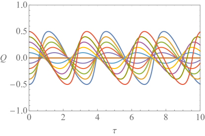
Figure 1: Projections of the time evolution of phase space trajectories along the $\Omega$-axis and $Q$-axis which determine the stability of point $P_{2}$. These panels are plotted for $\omega=\frac{1}{3}$.

To discuss the evolution of early universe, we have plotted the phase diagram of $(\Omega,Q)$ with different $\omega$ which are shown in Figs. 2 and  3. In these figures, the red points and lines denote the critical points, the purple dashed lines represent an example of the evolutionary curves of the universe.

For $\omega=1$, there exists two normally hyperbolic critical points $P_{4}$ and $P_{5}$ in the autonomous system, and both of them are a set of non-isolated points. $P_{4}$ denotes a stable contracting solution, while $P_{5}$ denotes an unstable expanding solution. So, the universe will evolve from an expanding phase to a contracting phase in this case, which is plotted in the left panel of Fig. 2.

For $-\frac{1}{3}<\omega<1$, there is three critical points $P_{1}$, $P_{2}$ and $P_{3}$ in the autonomous system. $P_{1}$ denotes a saddle point and corresponds to a contracting solution, $P_{2}$ denotes a stable Einstein static solution, and $P_{3}$ represents a saddle point and corresponds to an expanding solution. In this case, the universe is an oscillating universe, and it will become an Einstein static universe if we choose a special initial condition. This case is depicted in the right panel of Fig. 2.

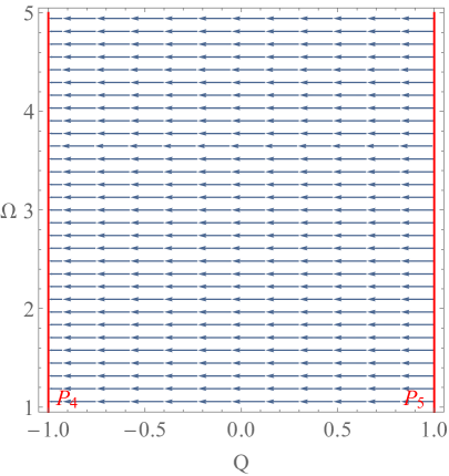
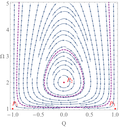
Figure 2: Phase diagram of $(\Omega,Q)$. These panels are plotted for $\omega=1$ and $\frac{1}{3}$, respectively. The red points and lines denote the critical points, the purple dashed lines represent the example of the evolutionary curves of the universe.

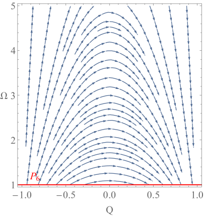
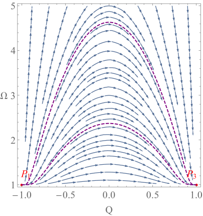
Figure 3: Phase diagram of $(\Omega,Q)$. These panels are plotted for $\omega=-\frac{1}{3}$ and $-\frac{2}{3}$, respectively. The red points and lines denote the critical points, the purple dashed lines represent the example of the evolutionary curves of the universe.

For $\omega=-\frac{1}{3}$, the autonomous system only has one normally hyperbolic critical point $P_{6}$ which is a set of non-isolated points. It is a stable expanding solution for $Q>0$, while it becomes an unstable contracting solution for $Q<0$. In this situation, the universe evolves from a contracting phase to an expanding phase, and it is a bouncing universe, which is depicted in the left panel of Fig. 3.

For $\omega<-\frac{1}{3}$, the autonomous system has two critical points $P_{1}$ and $P_{3}$. $P_{1}$ denotes an unstable contracting solution, while $P_{3}$ denotes a stable expanding solution. So, in this case, the universe will evolve from a contraction phase to an expanding phase, and it is a bouncing universe, which is shown in the right panel of Fig. 3.

Thus, the evolution of the early universe in Einstein-Cartan theory is determined by the initial conditions and the equation of state $\omega$, and there may exist a bouncing universe, an oscillating universe or an Einstein static universe in the early time of the universe.

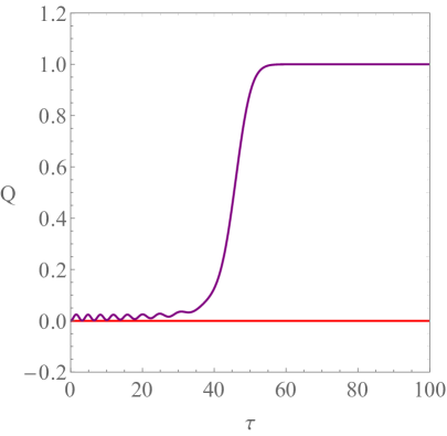
Figure 4: Evolutionary curve of $Q$ with time $\tau$. The red lines are plotted for $\omega=\frac{1}{3}$ with different initial values, while the purple lines are plotted for a time variable $\omega$. The red line in the left panel denotes an Einstein static universe, while the one in the right panel represents an oscillating universe.

According to the aforementioned results, we will describe the the evolution of early universe by assuming that the early universe filled by the radiation with $\omega=\frac{1}{3}$. So, the initial state of the early universe is an Einstein static or an oscillating universe.

If the initial state of universe is an Einstein static universe described by $P_{2}$, the evolution of the early universe can behave as the emergent universe. It is interesting to note that the stability conditions of $P_{2}$ are also obtained in Einstein static universe Atazadeh2014 and emergent universe HuangQ2015 . When the universe stems from an Einstein static universe and $\omega$ decreases to $-\frac{1}{3}$, the stability condition of the Einstein static solution $P_{2}$ is broken and $P_{2}$ changes from a stable state to an unstable state. As a result, the universe exits from a stable Einstein static state and becomes as an unstable Einstein static state, and then the universe will evolve into an expanding state described by $P_{3}$ eventually. In the left panel of Fig. 4, we have plotted this transition. In this figure, the red line denotes an Einstein static universe with $\omega=\frac{1}{3}$, $\Omega=2$ and $Q=0$, the purple line represents an emergent universe with a time variable $\omega$ which decreases with time $\tau$. We can see that when $\tau$ increases to a critical value, the universe exits from the Einstein static universe and evolves into an expanding phase. The detail procession is discussed in the emergent scenario HuangQ2015 .

If the initial state of universe is an oscillating universe and $\omega$ decreases to $-\frac{1}{3}$ which breaks down the oscillating conditions, the universe can also exit from the oscillating state and evolves into an expanding phase described by $P_{3}$. In the right panel of Fig. 4, we have plotted this evolutionary procession. In this figure, the red line denotes an oscillating universe with $\omega=\frac{1}{3}$, the purple line represents the evolutionary curve with a time variable $\omega$ which decreases with time $\tau$. We can see that when $\tau$ increases to a critical value, the universe exits from the oscillating universe and evolves into an expanding phase.

IV Conclusion

We find that there are eight different critical points, among which two critical points are physically meaningless because they leads to

Einstein-Cartan theory is a generalization of general relativity that introduces spacetime torsion, which can be equivalent to general relativity with an exotic stiff perfect fluid. In this paper, we analyze the evolution of the early universe in the Einstein-Cartan theory using the phase space analysis method. We find that there are eight different critical points, among which two critical points are physically meaningless because they leads to $\Omega_{s}=-1$. The stability of these critical points are mainly determined by the equation of state $\omega$. There exist two stable critical points $P_{2}$ and $P_{3}$. $P_{3}$ denotes an expanding solution and is stable for $\omega<-\frac{1}{3}$, while the stable Einstein static solution $P_{2}$ requires $-\frac{1}{3}<\omega<1$ and it is a center point. Therefore, $P_{3}$ can represent the final state of the evolution of the early universe.

After analyzing the phase diagram of the dynamical system and considering different initial conditions and the equation of state $\omega$, we find there may exist a bouncing universe, an oscillating universe or an Einstein static universe in the early time of the universe.

Furthermore, by assuming that the early universe filled by the radiation with $\omega=\frac{1}{3}$, the initial state of early universe is Einstein static universe or oscillating universe. If the initial state of the universe is an Einstein static universe described by $P_{2}$ and the equation of state $\omega$ can evolve with time and decrease to $-\frac{1}{3}$, the universe can exit from the static state and evolve into an expanding state described by $P_{3}$, and the evolution of early universe can behave as the emergent universe. If the initial state of the universe is an oscillating universe and $\omega$ decreases to $-\frac{1}{3}$, the universe can also exit from the oscillating state and evolves into an expanding phase described by $P_{3}$.

- (1) F. Hehl, P. von der Heyde, G. Kerlick, and J. Nester, Rev. Mod. Phys. 48, 393 (1976).
- (2) F. Hehl, Found. Phys. 15, 451 (1985).
- (3) F. Hehl, J. McCrea, E. Mielke, and Y. Neeman, Phys. Rep. 258, 1 (1995).
- (4) M. Lledo and L. Sommovigo, Class. Quantum Grav. 27, 065014 (2010).
- (5) J. Weyssenhoff and A. Raabe, Acta Phys. Pol. 9, 7 (1947).
- (6) Y. Obukhov and V. Korotky, Class. Quantum Grav. 4, 1633 (1987).
- (7) L. Smalley and J. Krisch, Class. Quantum Grav. 11, 2375 (1994).
- (8) G. de Berredo-Peixoto and E. De Freitas, Int. J. Mod. Phys. A 24, 1652 (2009).
- (9) B. Vakili and S. Jalalzadeh, Phys. Lett. B 726, 28 (2013).
- (10) F. Hehl, P. von der Heyde, and G. Kerlick, Phys. Rev. D 10, 1066 (1974).
- (11) I. Nurgaliev and W. Ponomariev, Phys. Lett. 130B, 378 (1983).
- (12) M. Gasperini, Phys. Rev. Lett. 56, 2873 (1986).
- (13) N. Poplawski, Gen. Relativ. Gravit. 44, 1007 (2012).
- (14) G. Unger and N. Poplawski, The Astrophysical Journal, 870, 78 (2019)
- (15) K. Atazadeh, JCAP 06, 020 (2014).
- (16) Q. Huang, P. Wu, and H. Yu, Phys. Rev. D 91, 103502 (2015).
- (17) N. Poplawski, Phys. Lett. B 694, 181 (2010).
- (18) N. Poplawski, Phys. Rev. D 83, 084033 (2011).
- (19) N. Poplawski, Phys. Rev. D 85, 107502 (2012).
- (20) K. Shie, J. Nester, and H. Yo, Phys. Rev. D 78, 023522 (2008).
- (21) A. Marco, E. Orazi, and G. Pradisi, Eur. Phys. J. C 84, 146 (2024).
- (22) M. He, K. Kamada, and K. Mukaida, JHEP 01, 014 (2024).
- (23) M. He, M. Hong, and K. Mukaida, ArXiv: 2402.05358.
- (24) M. Piani and J. Rubio, JCAP 05, 009 (2022).
- (25) M. Shaposhnikov, A. Shkerin, I. Timiryasov, and S. Zell, JCAP 02, 008 (2021).
- (26) M. Piani and J. Rubio, JCAP 12, 002 (2023).
- (27) F. Brandt, J. Frenkel, S. Martins-Filho, and D. McKeon, Annals Phys. 462, 169607 (2024).
- (28) R. Isichei and J. Magueijo, Phys. Rev. D 107, 023526 (2023).
- (29) M. Ranjbar, S. Akhshabi, and M. Shadmehri, ArXiv: 2401.02129.
- (30) E. Elizalde, F. Izaurieta, C. Riveros, G. Salgado, and O. Valdivia, Phys. Dark Univ. 40, 101197 (2023).
- (31) E. Battista and V. De Falco, Eur. Phys. J. C 82, 628 (2022).
- (32) E. Battista and V. De Falco, Phys. Rev. D 104, 084067 (2021).
- (33) S. Akhshabi and S. Zamani, Gen. Rel. Grav. 55, 102 (2023).
- (34) S. Soni, A. Khunt, and A. Hasmani, ArXiv: 2308.10612.
- (35) S. Hensh and S. Liberati, Phys. Rev. D 104, 084073 (2021).
- (36) B. Costa and Y. Bonder, Phys. Lett. B 849, 138431 (2024).
- (37) V. Falco, E. Battista, D. Usseglio, and S. Capozziello, Eur. Phys. J. C 84, 137 (2024).
- (38) V. Falco and E. Battista, Phys. Rev. D 108, 064032 (2023).
- (39) E. Battista, V. De Falco, and D. Usseglio, Eur. Phys. J. C 83, 112 (2023).
- (40) S. Bondarenko, S. Pozdnyakov, and M. Zubkov, Eur. Phys. J. C 81, 613 (2021).
- (41) N. Roy and N. Banerjee, Annals Phys. 356, 452 (2015).
- (42) J. Dutta, W. Khyllep, and N. Tamanini, Phys. Rev. D 93, 063004 (2016).
- (43) A. S. Bhatia and S. Sur, Int. J. Mod. Phys. D 26, 1750149 (2017).
- (44) J. Sola, A. Gomez-Valent, and J. de Cruz Perez, Mod. Phys. Lett. A 32, 1750054 (2017).
- (45) J. Guo and A. Frolov, Phys. Rev. D 88, 124036 (2013).
- (46) P. Wu and H. Yu, Phys. Lett. B 629, 176 (2010).
- (47) H. Wei, Phys. Lett. B 712, 430 (2012).
- (48) J. Dutta, W. Khyllep, E. Saridakis, N. Tamanini and S. Vagnozzi, JCAP 02, 041 (2018).
- (49) Q. Huang, R. Zhang, J. Chen, H. Huang, and F. Tu, Mode. Phys. Lett. A 36, 2150052 (2021).
- (50) M. Setare and E. Vagenas, Int. J. Mod. Phys. D 18, 147 (2009).
- (51) N. Banerjee and N. Roy, Gen. Relativ. Gravit 47, 92 (2015).
- (52) Q. Huang, H. Huang, J. Chen, L. Zhang, and F. Tu, Class. Quantum Grav. 36, 175001 (2019).
- (53) A. Bargach, F. Bargach, and T. Ouali, Nucl. Phys. B 940, 10 (2019).
- (54) Q. Huang, H. Huang, B. Xu, F. Tu, and J. Chen, Eur. Phys. J. C 81, 686 (2021).
- (55) H. Huang, Q. Huang, and R. Zhang, Gen. Relat. Gravit. 53, 63 (2021).
- (56) H. Huang, Q. Huang, and R. Zhang, Universe 8, 467 (2022).
- (57) A. Millano, K. Jusufi, and G. Leon, Phys. Lett. B 841, 137916 (2023).
- (58) C. Boehmer, N. Chan, and R. Lazkoz, Phys. Lett. B 714, 11 (2012).
- (59) J. Dutta, W. Khyllep, and N. Tamanini, Phys. Rev. D 95, 023515 (2017).
- (60) J. Dutta, W. Khyllep, and H. Zonunmawia, Eur. Phys. J. C 79, 359 (2019).
- (61) N. Roy and N. Bhadra, JCAP 06, 002 (2018).
- (62) J. Brannan, W. Boyce, and M. Mckibben, Differential Equations: An Introduction to Modern Methods and Applications, third edtion, Wiley, New York, p174-p175 (2015).