Convergence rate of the spectral difference method on regular triangular meshes
Abstract
We consider the spectral difference method based on the -th order Raviart – Thomas space () on regular triangular meshes for the scalar transport equation. The solution converges with the order if the transport velocity is parallel to a family of mesh edges and with the order otherwise. We prove this fact for and show it for in numerical experiments.
1 Introduction
The spectral difference (SD) method is a high order method for solving hyperbolic problems on unstructured meshes. Like in the discontinuous Galerkin (DG) method, a mesh function is a discontinuous piecewise -th order polynomial function, and a Riemann solver is used to calculate the numerical fluxes. The SD method attracts attention because of its simplicity compared to DG. Its main drawback is that SD is not based on a solid mathematical background. In particular, there is no -stability proof on unstructured meshes.
The spectral difference method was proposed for unstructured triangular meshes in [1, 2] and for quadrilateral meshes in [3, 4, 5, 6]. The stability in the 1D case was proved in [7]. However, it was found that for this scheme is unstable even on regular-triangular meshes [8]. This issue was overcome by the spectral difference method based on the Raviart – Thomas space (SD-RT), which was proposed for in [9]. It was generalized to in [10], to tetrahedral meshes in [11], and to mixed-element 3D meshes in [12].
In this paper we study the accuracy of the SD-RT method for the Cauchy problem for the transport equation
| (1) |
The transport velocity is constant, and the initial data is sufficiently smooth and periodic with the periodic cell .
The convergence rate in a quadratic norm of a stable -exact numerical method for (1) usually belongs to the range . For finite-difference schemes, there holds . On 1D non-uniform meshes, for both polynomial-based finite-volume schemes and the discontinous Galerkin method there holds .
On unstructured meshes, the situation becomes more complicated. The DG() method converges with the order under the minimal angle condition [13]. The -th order convergence is known if the angle between the mesh edges and the transport velocity is bounded from below [14]. The importance of this assumption was demonstrated by Peterson [15] who constructed a sequence of meshes where DG() converges with the order .
A similar effect holds for finite-volume schemes. On unstructured meshes, one usually observes a convergence rate close to [16]. But a lower convergence rate may happen. For instance, the convergence rates and were demostrated in a Peterson-type counterexample for 1-exact edge-based schemes [17].
Now we are concerned with the case of regular (also called translationally invariant, TI) triangular meshes, i. e. meshes that are invariant with respect to the translation by each edge. A triangular TI-mesh is the image of an infinite mesh of regular triangles mesh under a linear map. Two adjacent triangles form a periodic cell of the mesh, so each scheme on a triangular TI-mesh can be interpreted as a scheme with several degrees of freedom per cell on a uniform structured mesh. For a given direction of the transport velocity, the convergence rate of such schemes may be either or , see [18]. The -th order convergence of DG() in this case is a corollary of the -th order convergence. Finite-volume schemes also exhibit the -th order convergence provided that the dissipation is good enough so the checkerboard function shown at Fig. 1 is not a steady numerical solution.
In this paper we consider the SD-RT() method for the transport equation on translationally invariant triangular meshes, . We show that the numerical solution converges with the order if the transport velocity is parallel to a family of mesh edges and with the order otherwise. We prove this effect for and demonstrate it numerically for .

2 The SD-RT method
2.1 The Raviart – Thomas space
Let , , be the space of -th order polynomials of two variables. The Raviart – Thomas space of order is formally defined as
In particular,
Since , and the dimension of the space of homogeneous -order polynomials is , then . The divergence operator maps onto . For each and , the function is a -th order polynomial on each line orthogonal to . For more information about the Raviart – Thomas space see [19].
2.2 SD-RT on a general triangular mesh
Consider a triangular mesh in , periodic with the periodic cell . Let be the set of mesh triangles. A mesh function is a generally discontinuous piecewise-polynomial function, namely, , periodic with the periodic cell .
For each mesh edge, put points, for instance, at the knots of the Gauss – Legendre quadrature rule. On each triangle, define interior points. Together, they form the set of flux collocation points. For , on each , there is one interior point at the mass center. For , the location of interior points is chosen to enforce stability of the resulting scheme [9, 10], but there is no algorithm for a general .
By SD-RT() we denote the spectral difference method based on the Raviart – Thomas space of order . For the transport equation (1) it has the form
| (2) |
where is defined by the following conditions:
-
•
for each interior collocation point , , inside the triangle there holds
(3) -
•
for each flux collocation point on there holds
(4)
where is defined by solving the Riemann problem:
Here is the unit normal vector to the edge and are the limit values from both sides of the edge.
To define , we have vector equations and scalar equations, in total. Thus, the number of equations is equal to the number of unknowns. The non-degeneracy of this system is provided by the location of the interior collocation points.
Unless specifically stated, the initial data for the semidiscrete problem are given by
| (5) |
where is the Lagrangian mapping. Our results also hold if the orthogonal (in the sense of ) projection is used, see Remark 2.
By construction, SD-RT() is -exact in the sense of , i. e. for each the function , , satisfies (2).
Note that the replacement of (3) by
yields the discontinuous Galerkin method. For , there are no interior collocation points, so SD-RT(0) coincides with DG(0) and with the basic finite-volume method.
2.3 SD-RT(1) on a right-triangular mesh
Now we specify SD-RT(1) for a regular triangular mesh. Since an affine transform of the mesh together with the transport velocity keeps the scheme unmodified, we restrict our analysis to the meshes of right isosceles triangles.
Let the mesh nodes have radius-vectors , , , and the mesh edges connect each node to
The scheme coefficients are piecewise linear functions of , and their gradients are discontinuous when is parallel to a mesh edge. Without loss, we consider the case , .

Represent a mesh function on each triangle by its values at the vertices. Let . The point values at the vertices on the periodic cell of the mesh
are numerated as shown in Fig. 2. Denote them by . Then represents a mesh function.
In this notation, SD-RT(1) on the right-triangular mesh with step takes the form
| (6) |
where is the scheme stencil,
and are real-valued -matrices. The matrices have the form ,
The matrix results from by the permutation of rows 2 and 3, columns 2 and 3, rows 4 and 6, colunms 4 and 6: ,
Taking the linear interpolation from (6) within each triangle returns us to the form (2).
The Lagrangian mapping takes each to the function with the components
where is the radius-vector of solution point in block . The vectors are based on Fig. 2: , , , .
3 Criterion of the -th order convergence
Schemes of the general form (6), (5) were studied in [18]. We use the notation and some results from that paper. Throughout this section, is fixed.
Let be a multiindex: . Denote , , . For denote
| (7) |
Here means with the substitution . The vector is the coefficient at -th derivative in the truncation error of the scheme.
Equip the space of mesh functions with the norm
and use the Euclidean norm on . For , denote
The scheme is stable with constant if for each each -periodic solution of (6) satisfies . This holds iff
| (8) |
The solution error is where is the solution of (6) with the initial data , and . We say that the scheme has order if for each 1-periodic there holds with some and depending on . The optimal order of accuracy is the maximal value of such that this estimate holds.
The following proposition is a particular case of Theorem 3.1 in [18].
Proposition 1.
If , then the leading terms of the truncation error may be represented in a divergence form, which yields the -th order convergence. The second statement is more difficult to see. In [18], it was proved using the spectral analysis.
4 Accuracy analysis of SD-RT(1)
In this section, we study the accuracy of the SD-RT(1) scheme for (1) on the right-triangular meshes defined in Section 2.3. Throughout this section, , .
Our analysis is based on Proposition 1. To apply it, we need to know the stability, the co-kernel of the matrix , and some properties of .
4.1 Stability
The eigenvalues of
were studied numerically in [9]. It was shown that for each and each all eigenvalues have nonnegative real parts. To establish the stability we need a stronger statement.
Lemma 2.
For each there holds (8) with . As a corollary, the scheme is stable.
Proof.
Without loss, , , . We use Lapack to find the eigenvalues and eigenvectors of for all admissible with the step . The results show that all eigenvalues have nonnegative real parts, and the condition number of the matrix of eigenvectors does not exceed 32. ∎
4.2 Properties of
The matrix is defined as
General considerations give us the following information.
-
•
For each the vector belongs to the kernel of because the scheme is exact on a constant solution.
-
•
For each the vector belongs to the co-kernel of because the scheme is conservative.
-
•
If , then is a steady solution of (1). By 1-exactness, the vector also belongs to the kernel of .
We need to refine these results.
Lemma 3.
If , the co-kernel of is the span of . If , then the co-kernel of is the span of and .
Proof.
By the direct substitution, for non-degenerate matrices and defined by
there holds
If , then the last row of forms basis of the co-kernel of . If , then . It is easy to see that
Thus, belongs to the co-kernel of . ∎
4.3 Mean truncation error on the periodic cell
For , let be the piecewise-linear function on with point values at vertices assigned according to the numbering in Fig. 2. Then the orthogonality of and is equivalent to zero integral of over . Now we show that this condition holds.
Lemma 4.
For each and each such that there holds
Proof.
By the definition (7) of ,
| (9) |
Since is a first-order polynomial, then the map keeps it unmodified within . Therefore,
The coefficients in (6) are defined so that for each piecewise linear function and both triangles there holds
Taking this with to (9) we obtain
By the Gauss theorem,
where the sum is by edges of triangles from , and the unit normal is directed outwards. On each edge, the function is a first-order polynomial (see Section 2.1). By (4), it equals the upwind limit value of multiplied by . Thus,
We take the upper sign if and the lower sign otherwise. The edge located within the periodic cell counts twice with opposite normal direction and yields zero in sum. Since , then the function is 1-periodic. Thus, for each pair of opposite edges the expression in parentheses is the same, and the normals are opposite. Therefore, the sum by edges yields zero. ∎
Remark 1.
The proof of Lemma 4 extends to SD-RT() for each and to the discontinuous Galerkin method.
4.4 Main result
Theorem 5.
Proof.
If , then the vector forms the basis in the co-kernel of . The statement of the theorem follows from Proposition 1 and Lemma 4.
Consider the case . To evaluate the numerical derivative of a mesh function at the zeroth block, the scheme uses its values at and . At these points, the values of coincide with the values of . So the numerical derivative of at zeroth block is equal to the numerical derivative of , which is by -exactness. Thus,
Clearly, is not orthogonal to the vector , which belongs to the co-kernel of by Lemma 3. Hence, . By Proposition 1, the optimal order of accuracy is 1. ∎
Remark 2.
Up to this moment, we used the Lagrangian mapping . However, the statement of Theorem 5 holds for any local mapping (for instance, the orthogonal -projection) that coincides with on linear functions. Indeed, for each smooth there holds . If the scheme is second-order in the sense of , then by stability and the triangle inequality it is second-order in the sense of , and vice versa.
4.5 The long-time simulation accuracy
In this section we show that SD-RT(1) possesses the second order of accuracy in the long-time simulation for each . For , this follows from Theorem 5, so we need to consider the case only.
Lemma 6.
Let . Then the scheme (6) is 2-exact in the sense of taking each 1-periodic to the mesh function with the components
where for and otherwise, and for and otherwise.
The proof is by direct substitution, see Appendix A.
Corollary 7.
The proof is standard, so we give its sketch only.
5 Numerical results
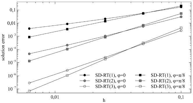
Now we apply SD-RT() with to the Cauchy problem for the transport equation (1) with the initial data and the transport velocitiy . We consider the cases and and use the right-triangular meshes described in Section 2.3. On the boundaries of the unit square, the periodic boundary conditions are set.
For the time integration, we use the 3-rd (for ) or the 4-th (for ) order Runge – Kutta method with the CFL number 0.1. So the error of the time integration is negligible.
For a triangle with vertices , , , define the solution collocation points as , , . For a given time, we measure the maximal difference between the numerical and the exact solution at the solution collocation points.
The numerical results at are shown in Fig. 3. We see the convergence with the order for and with the order for . This confirms the theoretical results proved for .
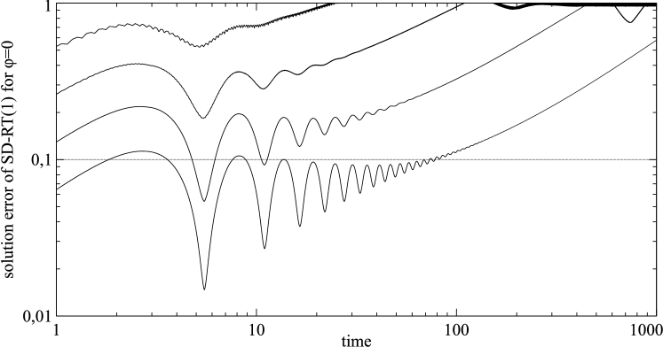
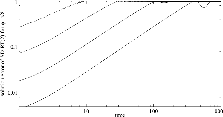
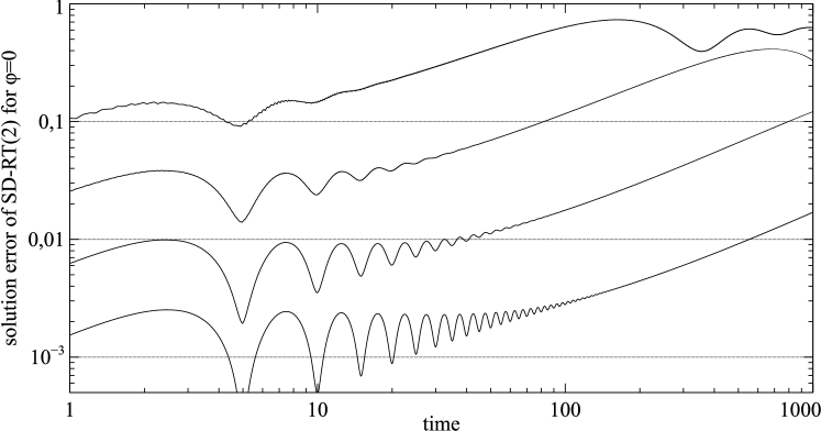
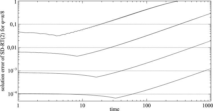
To study the long-time simulation accuracy, we plot the norm of the solution error as a function of time. The results are shown in Fig. 4 (, ), Fig. 5 (, ), Fig. 6 (, ), Fig. 7 (, ). Each line on each of these figures corresponds to a different (, , , ). We see that for a small time, the behavior of the solution error for differs from the case . However, for the distance between lines corresponding to different is identical for both cases and corresponds to the -th order convergence.
Appendix A How to get the coefficients of in Lemma 6
Here we present the code for the Sagemath package that was used to find the coefficients.
First set the matrices and .
L0 = matrix([[3,1,1,0,0,0],[-3,1,-2,0,0,0],[0,1,4,0,0,0],
[0,-1,-4,3,1,1],[0,2,2,-3,1,-2],[0,-4,-1,0,1,4]])
Lm = matrix([[0,0,0,0,-1,-4],[0,0,0,0,2,2],[0,0,0,0,-4,-1],
[0,0,0,0,0,0],[0,0,0,0,0,0],[0,0,0,0,0,0]])
Now set , , , , , .
e = vector((1,1,1,1,1,1)); x = vector((0,1,0,0,1,1)); y = vector((0,0,1,1,1,0))
xy = vector((0,0,0,0,1,0)); x2 = x; y2 = y
Indroduce the diagonal matrices , , with undetermined coefficients.
var(’c,d,b’)
Mx = diagonal_matrix([0,0,c,c,c,0])
My = diagonal_matrix([0,0,d,d,d,0])
Mxx = diagonal_matrix([b,0,0,b,0,0])
The form of and is defined by the 1-exactness of the scheme, and the addition of the diagonal matrix does not matter.
Now set , , , , , .
xp=x+Mx*e; yp=y+My*e; x2p = x2 + Mx*2*x + Mxx*2*e;
xyp = xy + Mx*y + My*x; y2p = y2 + My*2*y
Finally, write the truncation error on the quadratic polynomials in the sense of .
fxx = -2*xp + L0*x2p + Lm*(x2p-2*xp+e)
fxy = -yp + L0*xyp + Lm*(xyp-yp)
fyy = 0 + L0*y2p + Lm*y2p
The result is
Equating and to zero we obtain the coefficients: , , .
References
- [1] Liu Y., Vinokur M., Wang Z. J., Spectral difference method for unstructured grids I: basic formulation, Journal of Computational Physics 216 (2006) 780–801.
- [2] Wang Z. J., Liu Y., May G., Jameson A., Spectral difference method for unstructured grids II: Extension to the Euler equations, Journal of Scientific Computing 32 (2007) 45–71.
- [3] Sun Y., Wang Z. J., Liu Y., High-order multidomain spectral difference method for the Navier-Stokes equations on unstructured hexahedral grids, Communication in Computational Physics 2 (2007) 310–333.
- [4] Kuzmin M., Spectral difference method for the Euler equations on unstructured grids, Tech. Rep. WN-CFD-12-57, Centre Européen de Recherche et de Formation Avancée en Calcul Scientifique (2012).
- [5] Premasuthan S., Liang C., Jameson A., Computation of flows with shocks using spectral difference scheme with artificial viscosity, AIAA paper No 2010-1449 (2007).
- [6] Premasuthan S., Liang C., Jameson A., Computation of flows with shocks using the spectral difference method with artificial viscosity, II: Modified formulation and local mesh refinement, Computers and Fluids 98 (2014) 122–133.
- [7] Jameson A., A proof of the stability of the spectral difference method for all orders of accuracy, Journal of Scientific Computing 45 (2010).
- [8] Van den Abelee K., Lacor C., Wang Z.-J., On the stability and accuracy of the spectral difference method, Journal of Scientific Computing 37 (2008) 162–188.
- [9] Balan A., May G., Schoeberl J., A stable high-order spectral difference method for hyperbolic conservation laws on triangular elements, Journal of Computational Physics 231 (2012) 2359–2375.
- [10] Veilleux A., Puigt G., Hugues D., Daviller G., A stable spectral difference approach for computations with triangular and hybrid grids up to the 6 order of accuracy, Journal of Computational Physics 449 (2021).
- [11] Veilleux A., Puigt G., Hugues D., Daviller G., Stable spectral difference approach using Raviart-Thomas elements for 3D computations on tetrahedral grids, Journal of Scientific Computing 91 (2022).
- [12] G. Sáez-Mischlich, J. Sierra-Ausín, J. Gressier. The Spectral Difference Raviart–Thomas Method for Two and Three-Dimensional Elements and Its Connection with the Flux Reconstruction Formulation. Journal of Scientific Computing 93 (2022) 48. arXiv:2105.08632.
- [13] Johnson C., Pitkaränta J., An analysis of the discontinuous Galerkin method for a scalar hyperbolic equation, Mathematics of computation 46 (1986) 1–26.
- [14] Richter G. R., An optimal-order error estimate for the discontinuous Galerkin method, Mathematics of Computation 50 (1988) 75–88.
- [15] Peterson T. E., A note on the convergence of the discontinuous Galerkin method for a scalar hyperbolic equation, SIAM Journal of Numerical Analisys 28 (1991) 133–140.
- [16] Diskin B., Thomas J.-L., Comparison of node-centered and cell-centered unstructured finite-volume discretizations: Inviscid fluxes, AIAA Journal 49 (4) (2011) 836–854.
-
[17]
Bakhvalov P. A., Surnachev M. D.,
On the order of accuracy of
edge-based schemes. A Peterson-type counter-example, Communications on
Applied Mathematics and Computation (2023).
URL http://doi.org/10.1007/s42967-023-00292-8 - [18] Bakhvalov P. A., Surnachev M. D., Linear schemes with several degrees of freedom for the transport equation and the long-time simulation accuracy, IMA Journal of Numerical Analysis 44 (2024) 297–396.
- [19] F.-J. Sayas, From Raviart-Thomas to HDG (2013). arXiv:1307.2491.