Nonlinearity-enhanced quantum sensing in Stark probes

Abstract

Stark systems in which a linear gradient field is applied across a many-body system have recently been harnessed for quantum sensing. Here, we explore sensing capacity of Stark models, in both single-particle and many-body interacting systems, for estimating the strength of both linear and nonlinear Stark fields. The problem naturally lies in the context of multi-parameter estimation. We determine the phase diagram of the system in terms of both linear and nonlinear gradient fields showing how the extended phase turns into a localized one as the Stark fields increase. We also characterize the properties of the phase transition, including critical exponents, through a comprehesive finite-size scaling analysis. Interestingly, our results show that the estimation of both the linear and the nonlinear fields can achieve super-Heisenberg scaling. In fact, the scaling exponent of the sensing precision is directly proportional to the nonlinearity exponent which shows that nonlinearity enhances the estimation precision. Finally, we show that even after considering the cost of the preparation time the sensing precision still reveals super-Heisenberg scaling.

I Introduction

Due to extreme sensitivity to variations in environment, quantum systems can serve as sensors whose precision can exceed their classical counterparts [1, 2, 3, 4, 5, 6, 7, 8]. This superiority manifests itself in the uncertainty of their estimation, quantified by variance, which scales as ${~{}}L^{-\beta}$, where $L$ is probe size and $\beta$ is scaling exponent [9, 10, 11]. The best performance of the classical probes is limited to the standard quantum limit, namely $\beta{=}1$, determined by the central limit theorem. More favorable estimation precision with $\beta{>}1$ might be achievable through harnessing quantum features, e.g. entanglement, which is known as quantum-enhanced sensitivity. Originally, such enhancement was discovered for a probe made of non-interacting particles initialized in a certain type of entangled states, known as Greenberger-Horne-Zeilinger (GHZ) states [12, 13, 14, 15, 16, 17, 18, 19]. In GHZ-based sensors, the scaling of uncertainty improves to the Heisenberg limit, i.e. $\beta{=}2$. Nevertheless, susceptibility of those probes to decoherence [20, 21, 17, 22, 23, 24] and inter-particle interaction [25, 26] puts serious challenges for scaling up. Moreover, the precision of GHZ-based sensors with non-interacting particles is strictly bounded by the Heisenberg limit. To overcome these challenges, strongly correlated many-body systems, have been proposed as alternative types of sensors in which interaction between particles plays a central role. In particular, quantum criticality has been identified as a resource for achieving quantum-enhanced sensitivity. Several types of criticality have been used for achieving quantum enhanced sensitivity, including first-order [27, 28, 29], second-order [30, 31, 32, 33, 34, 35, 36, 37, 38, 39, 40, 41, 42, 43, 44, 45], dissipative [46, 47, 48, 49, 50, 51, 52, 53, 54, 55], time crystals [56, 57], Floquet [58, 59], topological [60, 61, 62, 63] and Stark phase transitions [64, 65]. The notion has also been generalized to non-Hermitian open quantum systems [66, 67, 68, 69].

Unlike GHZ-based sensors, the precision of criticality-based many-body probes is not bounded and super-Heisenberg scaling, namely $\beta{>}2$, may also be achievable [5, 32, 1, 6, 38, 39, 70]. However, the stringent requirement of initializing these probes in their ground state near the critical point, via, for instance, the adiabatic evolution, imposes difficulties in accessing this enhancement. As such, the possibility of exploiting the criticality turns to a hot debate in both theoretical [38] and experimental [41, 63, 71] arena. Recently, Stark many-body probes have been introduced for measuring linear gradient fields with an unprecedented precision of $\beta{\simeq}6$ [64, 65]. Emerging onsite off-resonance energy in the presence of a gradient field localizes the wave function of the particles even in the presence of strong interaction. This interesting phenomenon, known as Stark localization [72], has been subject of recent studies [73, 74, 75, 76, 77, 78, 78, 79, 80, 81, 82, 83, 84, 85, 86, 87, 88, 89, 90, 91, 92, 93, 94, 95, 96, 97] and has been observed in different experimental platforms including ion traps [98], optical lattices [99, 100], and superconducting simulators [101]. There are two key features that make the Stark probes very distinct from the other many-body sensors. First, their best performance is obtained for small fields which most probes fail to estimate. Second, the Stark transition takes place across the whole spectrum and thus the requirement of precise preparation of the ground state is relaxed. While the localization properties of nonlinear Stark systems have been studied in several works [89, 85, 86, 93], their potential as quantum sensors have not yet been explored.

In this work, we address this issue by investigating the sensing capability of the Stark probe for estimating both linear and nonlinear gradient fields. Thus, the problem naturally lies in the context of multi-parameter sensing [102, 44, 103, 104, 105]. We consider the single-particle case as well as the many-body interacting probe. The phase diagram of the system which denotes the transition from extended to localized phase is specified by all elements of the quantum Fisher information matrix with respect to linear and nonlinear gradient fields. Quantum-enhanced sensitivity is achievable throughout the extended phase. In the case of single-particle probes, one recovers $\beta{\simeq}6$ for linear gradient fields while the scaling exponent enhances to $\beta{\simeq}8$ for the nonlinear field. For many-body interacting probes, one achieves $\beta{\simeq}3$ and $\beta{\simeq}5$ for estimating linear and nonlinear gradient fields, respectively. In fact, we show that the exponent $\beta$ linearly increases with increasing nonlinearity. In addition, we fully characterize the critical properties of the probe through finite-size scaling analysis. Remarkably, the obtained quantum enhancement is still reachable even after considering the cost of preparation time.

The paper is organized as follows. We begin by recapitulating the theory of multi-parameter quantum estimation and laying the analytic arguments of relevance to this study in section II. The results for the single-particle Stark probe are presented in section III and followed by our analysis for the many-body interacting probe in section IV. After presenting the resource analysis in section V, we focus on assessing the uncertainty of simultaneous estimation of considered parameters in section VI. Finally in section VII, we provide a detailed discussion on the general effect of nonlinearity on the performance of the Stark probe in both single-particle and many-body interacting cases. The paper has been summarized in section VIII.

II Parameter estimation theory

In this section, we briefly review the concepts of estimation theory for multi-parameter quantum sensing [102, 44, 103, 104]. We consider a quantum probe described by a density matrix $\rho_{\boldsymbol{h}}$ with encoded unknown parameters $\boldsymbol{h}=\{h_{1},h_{2},...,h_{p}\}$. The precision of estimating $\boldsymbol{h}$ is quantified through a $p\times p$ covariance matrix $\boldsymbol{Cov}(\boldsymbol{h})$ with elements as $(\boldsymbol{Cov})_{ij}(\boldsymbol{h}){=}\langle h_{i}h_{j}\rangle-\langle h_{i}\rangle\langle h_{j}\rangle$. This matrix satisfies the multi-parameter quantum Cramér-Rao inequality

$$\boldsymbol{Cov}(\boldsymbol{h})\geqslant\frac{1}{M}\boldsymbol{\mathcal{F}_{Q}}^{-1}(\boldsymbol{h}),$$ (1)

where, $M$ is the number of samples, and $\boldsymbol{\mathcal{F}_{Q}}$ is the $p\times p$ Quantum Fisher Information (QFI) matrix. The elements of QFI matrix are given by [106]

$$(\boldsymbol{\mathcal{F}_{Q}})_{ij}(\boldsymbol{h})=\frac{1}{2}\text{Tr}[\rho_{\boldsymbol{h}}(L_{i}L_{j}+L_{j}L_{i})],$$ (2)

where the Hermitian operator $L_{i}$, known as the Symmetric Logarithmic Derivative (SLD), is defined as

$$\frac{\partial\rho_{\boldsymbol{h}}}{\partial h_{i}}=\frac{1}{2}(\rho_{\boldsymbol{h}}L_{i}+L_{i}\rho_{\boldsymbol{h}}).$$ (3)

For pure states, namely $\rho_{\boldsymbol{h}}{=}|\psi(\boldsymbol{h})\rangle\langle\psi(\boldsymbol{h})|$, the QFI matrix elements are simplified to

$$(\boldsymbol{\mathcal{F}_{Q}})_{ij}(\boldsymbol{h})=4\rm{Re}\left[\langle\partial_{\textit{i}}\psi|\partial_{\textit{j}}\psi\rangle-\langle\partial_{\textit{i}}\psi|\psi\rangle\langle\psi|\partial_{\textit{j}}\psi\rangle\right],$$ (4)

with $\partial_{\textit{i}}{=}\partial/\partial h_{i}$. In the case of single-parameter estimation, the Eq. (1) reduces to a scalar inequality of the form $\delta h_{1}^{2}{\geqslant}M^{-1}(\boldsymbol{\mathcal{F}_{Q}})_{11}^{-1}(\boldsymbol{h})$ with $\delta h_{1}^{2}{=}\langle h_{1}^{2}\rangle{-}\langle h_{1}\rangle^{2}$ denoting the variance. In this case, the bound can always be saturated, in the limit of a large number of samples $M$, using an optimal measurement basis given by the eigenvectors of the corresponding SLD operator $L_{1}$. However, in the case of multi-parameter estimation with $p{>}1$, the bound is not tight. Intuitively, this is due to the non-commutativity of the optimal measurements associated to different parameters. When $[L_{i},L_{j}]=0$, for all choices of $i$ and $j$, the SLD operators are simultaneously diagonalizable, and the saturation condition is satisfied. It turns out that weaker condition ${\rm Tr}(\rho_{\boldsymbol{h}}[L_{i},L_{j}]){=}0$ for all $i$ and $j$ is both necessary and sufficient for the multi-parameter quantum Cramér-Rao bound (1) to be attainable [102].

Note that Eq. (1) is a matrix inequality and to obtain a scalar inequality, one can multiply both sides with a positive weight matrix $\boldsymbol{W}$ and compute the trace

$$\text{Tr}[\boldsymbol{W}\boldsymbol{Cov}(\boldsymbol{h})]\geqslant M^{-1}\text{Tr}[\boldsymbol{W}\boldsymbol{\mathcal{F}_{Q}}^{-1}(\boldsymbol{h})].$$ (5)

The weight matrix $\boldsymbol{W}$ can be chosen to add any combination of the elements of the covariance matrix as a measure of total uncertainty on the left side of the above inequality. In particular, one can choose $\boldsymbol{W}{=}\mathbb{I}$ for which the total uncertainty becomes the summation of variances of all the parameters and is bounded through $\sum^{p}_{i=1}\delta h_{i}^{2}\geqslant M^{-1}{\rm Tr}[\boldsymbol{\mathcal{F}_{Q}}^{-1}(\boldsymbol{h})]$. If one is only interested in the precision of estimating $h_{i}$, the weight matrix $\boldsymbol{W}$ needs to be chosen with only one non-zero element, namely $(\boldsymbol{W})_{ii}{=}1$. In this case, Eq. (5) reduces to $\delta h_{i}^{2}{\geqslant}M^{-1}(\boldsymbol{\mathcal{F}_{Q}}^{-1}(\boldsymbol{h}))_{ii}$. On the other hand, if all the parameters from the set $\boldsymbol{h}$ are exactly known except $h_{i}$, the problem reduces to a single parameter estimation in which $\delta h_{i}^{2}{\geqslant}M^{-1}(\boldsymbol{\mathcal{F}_{Q}})_{ii}^{-1}(\boldsymbol{h})$. For any positive semi-definite matrix, such as $\boldsymbol{\mathcal{F}_{Q}}$, one can show that $(\boldsymbol{\mathcal{F}_{Q}}^{-1})_{ii}{\geqslant}(\boldsymbol{\mathcal{F}_{Q}})^{-1}_{ii}$ with equality being achieved if $\boldsymbol{\mathcal{F}_{Q}}$ is a diagonal matrix. This clearly shows that the simultaneous estimation of multiple parameters reaches the same performance as the separate estimation schemes only if there are no correlations between parameters.

III Single-particle Stark probe

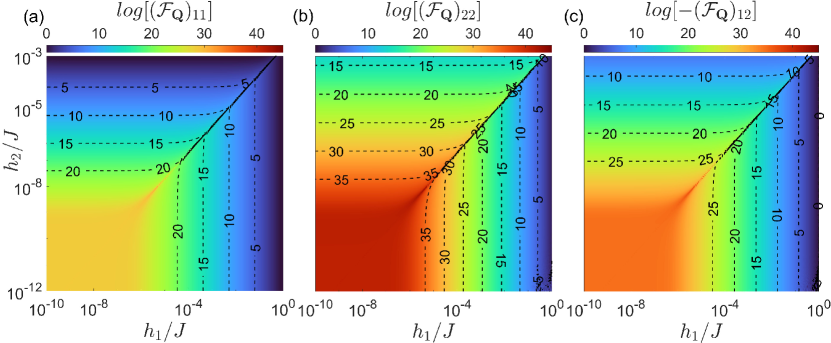
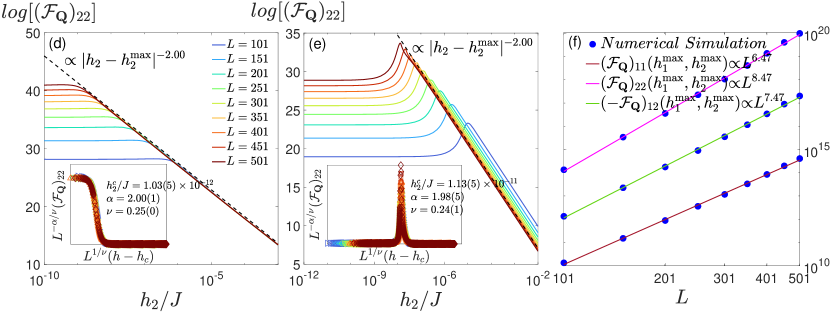
Figure 1: The QFI matrix elements, (a) ${\rm log}[(\boldsymbol{\mathcal{F}_{Q}})_{11}]$, (b) ${\rm log}[(\boldsymbol{\mathcal{F}_{Q}})_{22}]$ and (c) ${\rm log}[(-\boldsymbol{\mathcal{F}_{Q}})_{12}]$, as a function of linear $h_{1}$ and nonlinear $h_{2}$ terms of the potential landscape $V_{i}$, when the probe with size $L=501$ is prepared in the ground state. ${\rm log}[(\boldsymbol{\mathcal{F}_{Q}})_{22}]$ as a function of $h_{2}$ for a fixed value of (d) $h_{1}/J=10^{-8}$ and (e) $h_{1}=h_{2}(L-1)$. The dashed lines describe the algebraic decay of the Fisher information in the localized phase which is well-fitted by $|h_{2}-h_{2}^{\max}|^{-\alpha}$ with $\alpha{=}2.00$. The insets are the corresponding finite-size scaling analysis. The optimal data collapse is obtained for the reported $(h_{2}^{c},\alpha,\nu)$. Note that all the axes are in a logarithmic scale. (f) The maximum values of the QFI matrix elements (dots) as a function of probe size $L$. Lines are the best fitting function as $(\boldsymbol{\mathcal{F}_{Q}})_{ij}(h_{1}^{\max},h_{2}^{\max})\propto L^{\beta}$ to describe the scaling behaviour of the QFI matrix elements.

We begin by briefly recapitulating the physics of Stark localization transition in single-particle level. Consider a one-dimensional probe with $L$ sites in which the particle can tunnel between neighboring sites with rate $J>0$, in the presence of linear $h_{1}{>}0$ and nonlinear $h_{2}{>}0$ gradient fields which we would like to estimate. The total Hamiltonian of the system reads

$$H(h_{1},h_{2})=J\sum_{i=1}^{L-1}\left(|i\rangle\langle i+1|+h.c.\right)+\sum_{i=1}^{L}V_{i}(h_{1},h_{2})|i\rangle\langle i|,$$ (6)

where the potential $V_{i}$ is ,

$$V_{i}(h_{1},h_{2})=h_{1}(i-1)-h_{2}(i-1)^{2}.$$ (7)

In the absence of gradient fields, i.e. $V_{i}{=}0$, the Hamiltonian can be easily diagonalized which results in extended Bloch eigensystem as

$$E_{k} = -2J{\rm cos}(\frac{k\pi}{L+1})$$ (8)

$$|E_{k}\rangle = \sqrt{\frac{2}{L+1}}\sum_{j=1}^{L}(-1)^{j}\sin\left(\frac{jk\pi}{L+1}\right)|j\rangle,$$ (9)

where index $k{=}1,{\cdots},L$ counts all the eigenstates of the system. Clearly, in the absence of gradient fields $h_{1}$ and $h_{2}$, the eigenstates are extended across the entire system, known as the extended phase [74, 76]. In the presence of gradient fields $V_{i}{\neq}0$, the off-resonant energy splitting at each site tends to localize the wave function of the particle, known as Stark localization. It is well known that, the transition from the extended to the localized phase takes place across the entire spectrum for a gradient field that approaches zero in the thermodynamic limit ($L{\rightarrow}\infty$) [76, 96].

Recently, the Stark probe, in the linear regime, namely where $h_{2}{=}0$, has been exploited for sensing the gradient field $h_{1}$ [64, 65]. Three main results have been observed. First, all the eigenstates of the system show quantum-enhanced sensitivity, in terms of the system size $L$, with super-Heisenberg precision in the extended regime and transition point. Second, in the localized regime, the sensitivity becomes size independent and the system shows universal behavior. Third, the phase transition from the extended to the localized phase is described by a continuous second order phase transition formalism which implies the emergence of a diverging length scale at the transition point.

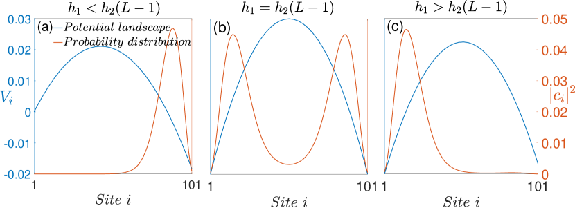
Figure 2: The potential landscape $V_{i}{=}h_{1}(i-1){-}h_{2}(i-1)^{2}$ and probability distribution of the ground state $|c_{i}|^{2}$, labeled on the left and right side of the plots, respectively, as a function of lattice site $i$ with probe size $L{=}101$. The values of the parameters are chosen as (a) $h_{1}{<}h_{2}(L-1)$, (b) $h_{1}{=}h_{2}(L-1)$, and (c) $h_{1}{>}h_{2}(L-1)$.

Relying on multi-parameter estimation theory, in this work we assess the performance of the Stark probe for estimating both linear and nonlinear gradient fields which compete to localize the system through their different signs. Note that, the opposite signs of $h_{1}$ and $h_{2}$ in $V_{i}$ create a parabolic potential landscape across the lattice. By focusing on the ground state of the Hamiltonian Eq. (6), we aim to estimate both the parameters $h_{1}$ and $h_{2}$. As the figure of merit, we compute the QFI matrix whose elements are plotted in Fig. 1. Since the QFI matrix is symmetric, one has $(\boldsymbol{\mathcal{F}_{Q}})_{12}{=}(\boldsymbol{\mathcal{F}_{Q}})_{21}$. In Figs. 1(a)-(c), we depict $(\boldsymbol{\mathcal{F}_{Q}})_{11}$, $(\boldsymbol{\mathcal{F}_{Q}})_{22}$ and $(\boldsymbol{\mathcal{F}_{Q}})_{12}$ as a function of $h_{1}$ and $h_{2}$ for the probe of size $L{=}501$, respectively. The phase diagram is indeed fully described by both $h_{1}$ and $h_{2}$. Several common features can be observed. By changing the parameters $(h_{1},h_{2})$, all the elements of the QFI matrix show a clear transition from the extended phase in which the Fisher information remains steadily high for small values of $h_{1}$ and $h_{2}$ (a rectangular region in the lower left corner of the phase diagram with hot color) to a localized phase in which the Fisher information significantly shrinks (regimes with cold colors). The Fisher information reveals a peak along the line $h_{1}{=}h_{2}(L-1)$ that represents the situation in which the Stark potential $V_{i}$ becomes symmetric around the center of the system, namely $V_{i}{=}V_{L-i+1}$. We come back to this interesting case later. To clarify this Stark localization transition in our probe, in Fig. 1(d) we plot $(\boldsymbol{\mathcal{F}_{Q}})_{22}$ versus $h_{2}$ for $h_{1}{=}10^{-8}J$ and different probe sizes. The QFI initially follows a plateau, indicating the extended phase, and then starts to decrease at a specific value of $h_{2}=h_{2}^{\max}$, which is size dependent. By increasing the size of the system, three important features can be observed. First, $h_{2}^{\max}$’s tend to smaller values signaling $h_{2}^{\max}{\rightarrow}h_{2}^{c}{=}0$ in the thermodynamic limit. Second, the value of the QFIs in the extended phase dramatically increases by increases the system size, hinting its divergence in the thermodynamic limit (i.e. $L{\rightarrow}\infty$). Third, in the localized phase the QFIs becomes size independent and shows a universal algebraic decay as ${\propto}|h_{2}-h_{2}^{\max}|^{-\alpha}$ with $\alpha{=}2.00$, see the dashed fitting line in the panel (d). Note that these three observations are valid for all the elements of the QFI matrix (data not shown). Similarly, one can fix $h_{2}$ into a small value and plot the elements of the QFI matrix as a function of $h_{1}$ which all show similar qualitative behavior, namely a size-dependent plateau followed by a universal size-independent behavior. This is analogous to the Stark localization transition observed for a single parameter [64, 65]. In Fig. 1(e), we investigate the behavior of the QFI along the symmetric line $h_{1}{=}h_{2}(L-1)$ for various system sizes. Interestingly, $(\boldsymbol{\mathcal{F}_{Q}})_{22}$ shows a peak at the transition from the extended to the localized phase. The emergence of peaks during the symmetric line can be observed in all the QFI matrix elements (shown as dark points on Figs. 1(a)-(c)). To elucidate the origin of this extra enhancement in the QFI elements, we note that for $h_{1}=h_{2}(L-1)$, one has $[H,\mathcal{M}]{=}0$, where $\mathcal{M}$ is the mirror operator defined as $\mathcal{M}|i_{1},\cdots,i_{L}\rangle{=}|i_{L},\cdots,i_{1}\rangle$. This implies that the eigenstates of the system are either symmetric, namely $\mathcal{M}|E_{k}\rangle{=}|E_{k}\rangle$, or anti-symmetric, namely $\mathcal{M}|E_{k}\rangle{=}{-}|E_{k}\rangle$, around the center of the chain. We conclude that the presence of this mirror symmetry is the origin of the extra sensitivity that one observes in Figs. 1(e). For the sake of completeness, we also investigate the wave function of the ground state $|E_{1}\rangle{=}\sum_{i}c_{i}|i\rangle$ for arbitrary values of $V_{i}$. In Figs. 2(a)-(c), both $V_{i}$ and $|c_{i}|^{2}$ as a function of lattice site $i$ and in three different regimes are presented. The mirror symmetry of the ground state for $h_{1}{=}(L-1)h_{2}$, see Fig. 2(b), results in the bilocalization of the particle in both edges of the system. By getting distance from the symmetric line, for instance in regimes with $h_{1}{<}(L-1)h_{2}$ or $h_{1}{>}(L-1)h_{2}$, the mirror symmetry breaks and, hence, $[H,\mathcal{M}]{\neq}0$, therefore the particle fully localize in either left or right side of the chain, see Figs. 2(a) and (c).

To determine the quantum enhancement in terms of the system size, in Fig. 1(f) we plot the maximum values of the QFI matrix elements along the symmetric line $h_{1}{=}h_{2}(L-1)$ as a function of the probe size. Clearly, the numerical simulations (markers) are well defined by a fitting function of the form $(\mathcal{F}_{Q})_{ii}{}\propto L^{\beta_{i}}$ (solid lines). Interestingly all the QFI matrix elements provide super-Heisenberg scaling as $(\boldsymbol{\mathcal{F}_{Q}})_{11}{\propto}L^{6.47}$, $(\boldsymbol{\mathcal{F}_{Q}})_{22}{\propto}L^{8.47}$, and $(-\boldsymbol{\mathcal{F}_{Q}})_{12}{\propto}L^{7.47}$. To describe the Stark transition, we rely on the second-order phase transition framework which suggests that the QFI matrix elements satisfy the following ansatz

$$(\boldsymbol{\mathcal{F}_{Q}})_{ii}=L^{\alpha_{i}/\nu_{i}}\mathcal{G}_{i}(L^{1/\nu_{i}}(h-h_{c}))$$ (10)

where $\mathcal{G}_{i}(\bullet)$ is an arbitrary function and $\alpha_{i}$ and $\nu_{i}$ are critical exponents. One can extract the critical exponents through finite-size scaling analysis in which the quantity $L^{\alpha_{i}/\nu_{i}}(\boldsymbol{\mathcal{F}_{Q}})_{ii}$ is plotted versus $L^{1/\nu_{i}}(h-h_{c})$ for various system sizes. By varying the critical exponents, one can collapse the curves of different sizes. In the inset of Fig. 1(d), the corresponding data collapse for $(\mathcal{F}_{Q})_{22}$ is obtained for $(h_{2}^{c},\alpha_{2},\nu_{2}){=}(1.03{\times}10^{-12}J,2.00,0.25)$. Similarly, for the transition along the symmetry line, the data collapse shown in the inset of Fig. 1(e) is obtained for $(h_{2}^{c},\alpha_{2},\nu_{2}){=}(1.10{\times}10^{-11}J,1.98,0.24)$. Applying the finite-size scaling analysis for $(\mathcal{F}_{Q})_{11}$ results in $(h_{1}^{c},\alpha_{1},\nu_{1}){=}(1.14{\times}10^{-10}J,1.99,0.31)$ and $(h_{1}^{c},\alpha_{1},\nu_{1}){=}(1.02{\times}10^{-10}J,1.99,0.33)$ for the transition during the symmetric line and beyond it. For the obtained critical parameters, one can check the validity of $\beta_{i}{=}\alpha_{i}/\nu_{i}$ (for $i{=}1,2$) which shows that the critical exponents are not independent of each other, see Ref. [64] for more details.

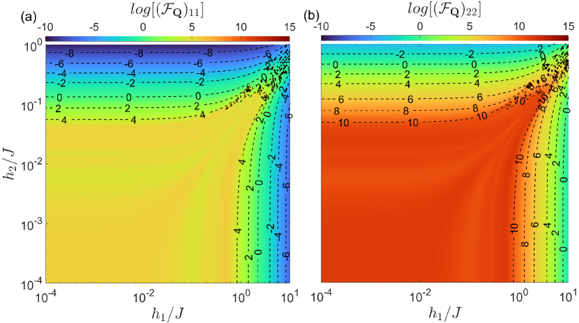
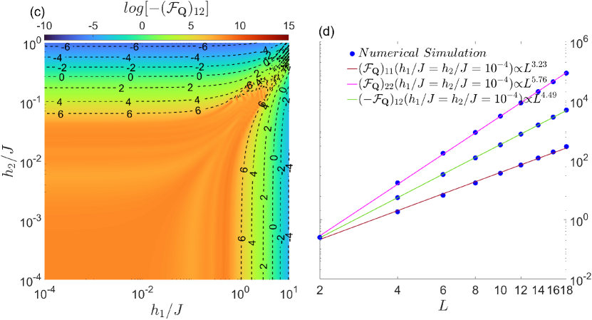
Figure 3: The QFI matrix elements, (a) ${\rm log}[(\boldsymbol{\mathcal{F}_{Q}})_{11}]$ and (b) ${\rm log}[(\boldsymbol{\mathcal{F}_{Q}})_{22}]$, as a function of $h_{1}$ and $h_{2}$ when the many-body interacting probe (Eq. (11)) with size $L=18$ is prepared in its ground state. (d) the values of the QFI matrix elements at $(h_{1}{=}h_{2}{=}10^{-4}J)$ (deep in the delocalized phase) as a function of the probe size. The numerical results are properly described by a fitting function as $(\boldsymbol{\mathcal{F}_{Q}})_{ij}(h_{1},h_{2})\propto L^{\beta}$ with reported $\beta$’s.

IV Many-body interacting probes

Quantum many-body probes exploit interaction between particles to enhance their sensitivity. This is in sharp contrast to interferometry-based quantum sensing in which interaction deteriorates the sensitivity. Therefore, it is worth studying many-body effects and the role of interaction on the performance of our Stark probe. We start by considering a probe of size $L$ in the half-filling regime where $N{=}L/2$ particles interact with each other based on the following Hamiltonian

$$H(h_{1},h_{2})=J\sum_{i=1}^{L-1}\boldsymbol{\sigma_{i}\cdot\sigma_{i+1}}+\sum_{i=1}^{L}V_{i}(h_{1},h_{2})\sigma_{i}^{z},$$ (11)

where $\boldsymbol{\sigma_{i}}{=}(\sigma_{i}^{x},\sigma_{i}^{y},\sigma_{i}^{z})$ and $\sigma_{i}^{x,y,z}$ are the Pauli operators acting at site $i$. The half filling subspace is defined by $\langle S_{z}^{tot}\rangle{=}\langle\sum_{i}^{L}\sigma^{z}_{i=1}\rangle{=}0$. To evaluate the probe’s performance, we calculate the QFI matrix for the ground state of systems up to size $L{=}18$, obtained using exact diagonalization. The results are presented in Figs. 3(a)-(c). Similar to the single-particle probe, by varying $h_{1}$ and $h_{2}$ from small to large values, the QFI matrix elements change remarkably from a region where their value remains steady (the area with warm colors) in the delocalized phase to a region where their values decrease monotonically (the area with cold colors) in the localized phase. Although the finite-size effect in many-body interacting probes results in a wider area for the extended phase, by increasing the size of the system this area shrinks until eventually vanishes at the thermodynamic limit. Considering the strong finite-size effect on the results, extracting the scaling behavior in the vicinity of the phase boundaries is very challenging. Therefore, in Fig. 3(d), we focus on the delocalized phase and plot the value of QFI matrix elements at $h_{1}{=}h_{2}{=}10^{-4}J$. The numerical results (markers) are well-describe by the fitting function as $(\boldsymbol{\mathcal{F}_{Q}})_{ij}\propto L^{\beta}$ (solid line) with $\beta{>}2$ for all QFI matrix elements. The exact values for $h_{1}{=}h_{2}{=}10^{-4}J$ are obtained as $(\boldsymbol{\mathcal{F}_{Q}})_{11}{\propto}L^{3.23}$, $(\boldsymbol{\mathcal{F}_{Q}})_{22}{\propto}L^{5.76}$, and $(-\boldsymbol{\mathcal{F}_{Q}})_{12}{\propto}L^{4.49}$. These results guarantee that similar to the single-particle probe, the many-body interacting probe can also offer quantum-enhanced sensitivity.

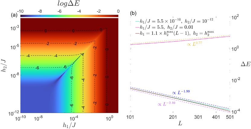
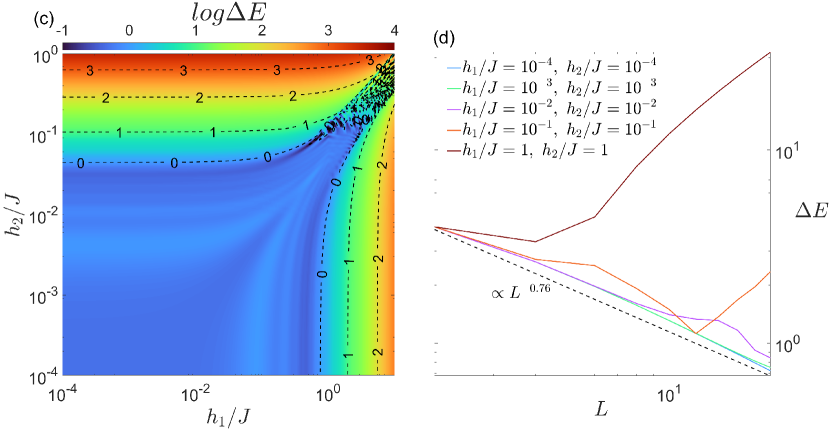
Figure 4: The energy gap between ground state and the first-excited state $\Delta E$ as a function of $h_{1}$ and $h_{2}$ for (a) single-particle probe with size $L=501$; and (c) many-body interacting probe with size $L=20$. (b) and (d) the energy gap as a function of probe size $L$ for different choices of $h_{1}$ and $h_{2}$ in single-particle and many-body interacting probes, respectively. The dashed black lines are eye guides that describe the decreasing behavior as $\Delta E{\sim}L^{-z}$.

V Resource analysis

As discussed above, the ground state of Stark probes can achieve quantum-enhanced sensitivity. So far, in our analysis, we have considered the probe size $L$ as the relevant resource for achieving such enhanced precision. However, preparation of the ground state might be challenging and time-consuming. Therefore, one may include the time $t$ which is needed to prepare the probe in its ground state as another resource. In order to incorporate time into our resource analysis, we use the normalized QFI matrix $t^{-1}\boldsymbol{\mathcal{F}_{Q}}(\boldsymbol{h})$ as a figure of merit. To estimate the time $t$, we consider adiabatic state preparation in which one can slowly evolve the probe from a simple ground state into the desired one. To avoid emergence of excited states during this evolution and guarantee that the system ends up in the desired ground state, the quench rate of the parameters needs to be adequately small, namely $t\sim 1/\Delta E$ with $\Delta E$ being the lowest energy gap during the variation of the Hamiltonian [107]. When the system is adiabatically evolved nearby a phase transition point, the minimum energy gap at the criticality scales as $\Delta E{\sim}L^{-z}$ [38], where $z$ is known as the dynamical critical exponent. Therefore, the time required for state preparation is $t\sim L^{z}$. In Fig. 4(a), we plot the energy gap between the ground state and the first excited state $\Delta E$ as a function of $h_{1}$ and $h_{2}$ for the single-particle probe of size $L{=}501$. By moving from the extended phase to the localized one, the energy gap $\Delta E$ increases. Fig. 4(b) illustrates the obtained $\Delta E$ for different sizes of the probe, in three points including deep in the extended phase, namely $h_{1}{=}5.5\times 10^{-10}J$ and $h_{2}{=}10^{-12}J$, near the transition point ($h_{1}^{\max},h_{2}^{\max}$), and deep in the localized side, namely $h_{1}{=}5.5J$ and $h_{2}{=}0.01J$. Not that to avoid the ground-state degeneracy in the transition point ($h_{1}^{\max},h_{2}^{\max}$) which is across the symmetric line $h_{1}=h_{2}(L-1)$, we focus on $h_{1}=1.1\times h_{2}(L-1)$. In both the extended phase and near the transition points, one has $\Delta E{\propto}L^{-1.99}$ and $\Delta E{\propto}L^{-2.10}$, respectively, which is in agreement with our previous observations [64]. However, the energy gap becomes positively correlated to the probe size as $\Delta E{\propto}L^{0.77}$ in the localized phase, which might be beneficial to the state initialization. Based on this result the ultimate scaling of the QFI matrix elements is obtained as $t^{-1}(\boldsymbol{\mathcal{F}_{Q}})_{11}(h_{1}^{\max},h_{2}^{\max}){\propto}L^{4.37}$, $t^{-1}(\boldsymbol{\mathcal{F}_{Q}})_{22}(h_{1}^{\max},h_{2}^{\max}){\propto}L^{6.37}$, and $t^{-1}(-\boldsymbol{\mathcal{F}_{Q}})_{12}(h_{1}^{\max},h_{2}^{\max}){\propto}L^{5.37}$, confirming the quantum-enhancement in the achievable precision. The same analysis can be done for the many-body interacting probe. In Fig. 4(c), the energy gap $\Delta E$ as a function of $h_{1}$ and $h_{2}$ for a probe of size $L{=}20$ is reported. Again, increasing the parameters widens the energy gap between the ground state and the first excited state. Extracting the dynamical critical exponent through studying $\Delta E$ versus $L$ in Fig. 4(d) results in $z{\sim}0.76$ for a many-body probe that works deeply in the delocalized phase. This results in the following normalization for the QFI matrix elements as $t^{-1}(\boldsymbol{\mathcal{F}_{Q}})_{11}(h_{1}{=}h_{2}{=}10^{-4}J){\propto}L^{2.47}$, $t^{-1}(\boldsymbol{\mathcal{F}_{Q}})_{22}(h_{1}{=}h_{2}{=}10^{-4}J){\propto}L^{5.00}$, and $t^{-1}(-\boldsymbol{\mathcal{F}_{Q}})_{12}(h_{1}{=}h_{2}{=}10^{-4}J){\propto}L^{3.73}$. Obviously, the quantum-enhancement can still be achieved even after considering the time that one needs to spend for initializing the probe.

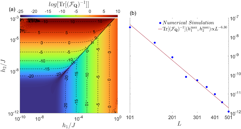
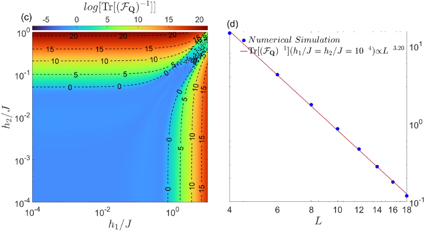
Figure 5: Total uncertainty ${\rm Tr}[(\boldsymbol{\mathcal{F}_{Q}})^{-1}]$ for the equally weighted multi-parameter estimation, as a function of $h_{1}$ and $h_{2}$ for (a) single-particle probe and (c) many-body interacting probe prepared in the corresponding ground state. (b) and (d) ${\rm Tr}[(\boldsymbol{\mathcal{F}_{Q}})^{-1}]$ versus $L$ for single-particle probes at $(h_{1}^{\max},h_{2}^{\max})$, and many-body interacting probes at $h_{1}{=}h_{2}{=}10^{-4}J$, respectively. The Numerical simulation (markers) are well describe by a fitting function as ${\rm Tr}[(\boldsymbol{\mathcal{F}_{Q}})^{-1}]{\propto}L^{-\beta}$ with $\beta=6.3$ for single-particle probe and $\beta=3.2$ for many-body interacting one.

VI multi-parameter Estimation

Up to now, we only focus on the performance of the Stark probes by studying the QFI matrix elements. Despite the differences in these elements, their behavior in the extended and localized phases, as well as at the transition point look similar. This hints that the Stark probe can potentially realize a multi-parameter estimation scenario. Back to Eq. (5), one can establish an equally weighted multi-parameter estimation by choosing $\boldsymbol{W}{=}\mathbb{I}$ and calculating $\text{Tr}[\boldsymbol{\mathcal{F}_{Q}}^{-1}(\boldsymbol{h})]$ as the ultimate estimation precision that lower bound total uncertainty

$$\delta h_{1}^{2}{+}\delta h_{2}^{2}\geq\text{Tr}[\boldsymbol{\mathcal{F}_{Q}}^{-1}(\boldsymbol{h})]=\frac{(\boldsymbol{\mathcal{F}_{Q}})_{11}+(\boldsymbol{\mathcal{F}_{Q}})_{22}}{(\boldsymbol{\mathcal{F}_{Q}})_{11}(\boldsymbol{\mathcal{F}_{Q}})_{22}-(\boldsymbol{\mathcal{F}_{Q}})_{12}(\boldsymbol{\mathcal{F}_{Q}})_{21}}$$ (12)

Our results for $\text{Tr}[\boldsymbol{\mathcal{F}_{Q}}^{-1}(h_{1},h_{2})]$ is presented in Fig. 5(a) for single-particle probe of size $L{=}501$. Obviously, the lowest uncertainty is obtained in the extended phase as well as along the symmetric line. As Eq. (12) shows, the nonvanishing off-diagonal elements of the QFI matrix $(\boldsymbol{\mathcal{F}_{Q}})_{12}{=}(\boldsymbol{\mathcal{F}_{Q}})_{21}$, affect the precision of multi-parameter estimation. This shows that the total uncertainty in simultaneous estimation of both linear and nonlinear terms of $V_{i}$ is larger than the case of estimating them individually as

$$\text{Tr}[\boldsymbol{\mathcal{F}_{Q}}^{-1}(\boldsymbol{h})]\geq\frac{1}{(\boldsymbol{\mathcal{F}_{Q}})_{11}}+\frac{1}{(\boldsymbol{\mathcal{F}_{Q}})_{22}}$$ (13)

This correlation effect shows itself properly in the scaling behavior of the probe. In Fig. 5(b), we report the lowest values of $\text{Tr}[\boldsymbol{\mathcal{F}_{Q}}^{-1}]$ which happens at $(h_{1}^{\max},h_{2}^{\max})$ for system of different sizes. The behavior of the numerical results (markers) can approximately be described by the fitting function $\text{Tr}[\boldsymbol{\mathcal{F}_{Q}}^{-1}]{\propto}L^{-\beta}$ with $\beta{=}6.30$. Regarding many-body probes, in Fig. 5(c) we plot $\text{Tr}[\boldsymbol{\mathcal{F}_{Q}}^{-1}]$ for a many-body probe of size $L{=}18$. Clearly, the lowest uncertainty can be obtained in the delocalized regime. In Fig. 5(d) we report $\text{Tr}[\boldsymbol{\mathcal{F}_{Q}}^{-1}]$ (markers) of different probe sizes obtained for parameters deep in the delocalized phase, namely $h_{1}{=}h_{2}{=}10^{-4}J$. The solid line is the best fitting function of the form $\text{Tr}[\boldsymbol{\mathcal{F}_{Q}}^{-1}]{\propto}L^{-\beta}$ with $\beta{=}3.20$. In the multi-parameter estimation scenario, despite the effect of the correlation between the parameters on the uncertainty of their estimation, another challenge is the saturation of the Cramér-Rao bound, namely finding a set of measurement that is optimized respect to the all unknown parameters. As has been discussed before, this relies on the satisfaction of either $[L_{i},L_{j}]{=}0$ or $\text{Tr}(\rho_{\boldsymbol{h}}[L_{i},L_{j}]){=}0$. One of the striking property of our model is that, while SLD operators do not satisfy the former except for $h_{1}{=}(L-1)h_{2}$, they always satisfy the latter one. This implies that there is always a set of optimized measurements that guarantee the saturation of the Cramér-Rao bound.

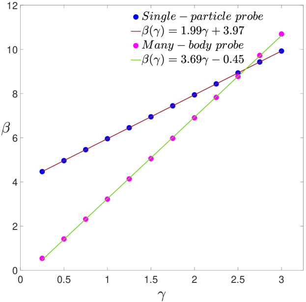
Figure 6: The extracted exponent $\beta$’s, governing the divergence of QFI as $\mathcal{F}_{Q}\propto L^{\beta}$, as a function of the nonlinearity $\gamma$ for both single-particle and many-body interacting probes, prepared in the ground state. The numerical simulation (markers) are fitted by a linear function $\beta(\gamma)=a\gamma+b$ (solid lines), with $(a,b){\sim}(1.99,3.97)$ for single-particle probe, $(a,b){\sim}(3.69,-0.45)$ for many-body interacting probe.

VII Effect of nonlinearity

Having elucidated the effect of parabolic potential landscape across the chain on the precision of estimation, in this section we aim to expand our study to a wider range of nonlineraities. To this end, we replaced $V_{i}(h_{1},h_{2})$ in Eqs. (6) by a potential landscape of form $V_{i}=hi^{\gamma}$ with $\gamma$ determining the nonlinearity. In particular, we focus on $\gamma\in[0.25,3]$. In this scenario, $h$ is the only parameter to estimate and thus we are back to single parameter estimation framework. To assess the role of the nonlinearity in a single-particle probe, for each given value of $\gamma$ and different system sizes $L\in\{101,\cdots,501\}$, we calculate the QFI as a function of $h$ for a probe initialized in the relevant ground state. Picking the highest value of the QFI which appear at the transition point $h^{\max}$ and analysing its behaviour respect to $L$, results

$$\mathcal{F}_{Q}(\gamma,h^{\max})\propto L^{\beta(\gamma)}.$$ (14)

The extracted $\beta$’s as a function of $\gamma$ is presented in Fig. 6. Obviously, the numerical results (markers) are well-described by fitting function

$$\beta(\gamma)\simeq a\gamma+b,$$ (15)

with $(a,b){\simeq}(1.99,3.97)$ for a single-particle probe that tuned to operate in its transition point. Applying the same analysis for the many-body interacting probe results in qualitatively similar behavior as Eq. (15) with $(a,b){\sim}(3.69,-0.45)$. In this case the $\beta$’s are obtained from analysing many-body interacting systems of size $L\in\{4,\cdots,16\}$. Several important observation need to be highlighted. First, by increasing nonlinearity the performance of the Stark probe improves. The origin of this improvement is the enhancement in the off-resonant energy splitting between neighboring sites. While $\Delta V_{i}(\gamma{=}1){=}V_{i+1}{-}V_{i}{=}h$, one has $\Delta V_{i}(\gamma{=}2){=}(2i{+}1)h$. This increase in the off-resonant energy splitting not only elevates the distingushablity of the energy difference but also boosts the power of localization in a way that transition point vanishes even in finite size systems. Second, in single-particle probes, quantum-enhanced sensitivity can be obtained for all values of $\gamma$ while in many-body probes it can only be achieved for $\gamma{>0.5}$. Third, the nonlinearity of the gradient field plays stronger role in the many-body probe and results in sharper growth of $\beta$ in comparison with the single-particle probe. This hints that for $\gamma>2.5$, a many-body probe operates better for reasonable large system sizes.

VIII Conclusion

The capability of Stark probes has already been identified for measuring linear tiny gradient fields with unprecedented precision, well beyond the capacity of most known critical-based sensors. In this work, we investigate the ability of these probes in providing extra enhancement in the presence of nonlinear Stark fields. As such, we applied a potential, containing both linear field $h_{1}$ and nonlinear field $h_{2}$ on the probe and simultaneously estimate them. The performance of the probe shows quantum enhanced sensitivity, with super-Heisenberg scaling, in both single excitation and half filling sectors for all the elements of the QFI matrix. In the single-particle Stark probe, the estimation precision of $h_{1}$ recovers the previous results with scaling exponent $\beta{\simeq}6$, while nonlinearity boosts the precision of the probe in estimating $h_{2}$ to $\beta{\simeq}8$. Having depicted the phase diagram for all elements of the QFI matrix with respect to $(h_{1},h_{2})$, we show that for $h_{1}{=}h_{2}(L-1)$ the emergence of a mirror symmetry in the system can enhance the precision of estimation. In many-body interacting probes, the corresponding scaling exponent for estimating $h_{1}$ and $h_{2}$ becomes $\beta{\simeq}3$ and $\beta{\simeq}5$, respectively. Furthermore, our results show that the scaling exponent $\beta$ for the QFI depends linearly on the nonlinearity exponent $\gamma$ as $\beta{\simeq}a\gamma+b$ with $a,b{\in}\mathbb{R}$ and $a{>}0$ independent of $L$. This clearly shows that nonlinearity can directly contribute to the quantum-enhanced sensitivity of Stark probes. Interestingly, quantum-enhanced sensitivity remains valid even if one incorporates the preparation time in our figure of merit.

IX Acknowledgement

A.B. acknowledges support from the National Natural Science Foundation of China (Grants No. 12050410253, No. 92065115, and No. 12274059), and the Ministry of Science and Technology of China (Grant No. QNJ2021167001L). R. Y. acknowledges support from the National Science Foundation of China for the International Young Scientists Fund (Grant No. 12250410242). A. C. acknowledges financial support from European Union NextGenerationEU through project PRJ-1328 “Topological atom-photon interactions for quantum technologies” (MUR D.M. 737/2021) and project PRIN 2022-PNRR P202253RLY “Harnessing topological phases for quantum technologies”.

References

- Roy and Braunstein [2008] S. Roy and S. L. Braunstein, Exponentially enhanced quantum metrology, Phys. Rev. Lett. 100, 220501 (2008).
- Paris [2009] M. G. Paris, Quantum estimation for quantum technology, Int. J. Quantum Inf. 7, 125 (2009).
- Banaszek et al. [2009] K. Banaszek, R. Demkowicz-Dobrzański, and I. A. Walmsley, Quantum states made to measure, Nat. Photon. 3, 673 (2009).
- Braun et al. [2018] D. Braun, G. Adesso, F. Benatti, R. Floreanini, U. Marzolino, M. W. Mitchell, and S. Pirandola, Quantum-enhanced measurements without entanglement, Rev. Mod. Phys. 90, 035006 (2018).
- Boixo et al. [2007] S. Boixo, S. T. Flammia, C. M. Caves, and J. M. Geremia, Generalized limits for single-parameter quantum estimation, Phys. Rev. Lett. 98, 090401 (2007).
- Beau and del Campo [2017] M. Beau and A. del Campo, Nonlinear quantum metrology of many-body open systems, Phys. Rev. Lett. 119, 010403 (2017).
- Degen et al. [2017] C. L. Degen, F. Reinhard, and P. Cappellaro, Quantum sensing, Rev. Mod. Phys. 89, 035002 (2017).
- Yousefjani et al. [2017a] R. Yousefjani, S. Salimi, and A. Khorashad, Enhancement of frequency estimation by spatially correlated environments, Ann. Phys. 381, 80 (2017a).
- Rao [1992] C. R. Rao, Information and the accuracy attainable in the estimation of statistical parameters, in Breakthroughs in statistics (Springer, 1992) pp. 235–247.
- Braunstein and Caves [1994] S. L. Braunstein and C. M. Caves, Statistical distance and the geometry of quantum states, Phys. Rev. Lett. 72, 3439 (1994).
- Cramér [1999] H. Cramér, Mathematical methods of statistics (Princeton university press, 1999).
- Greenberger et al. [1989] D. M. Greenberger, M. A. Horne, and A. Zeilinger, Going beyond Bell’s theorem, in Bell’s theorem, quantum theory and conceptions of the universe (Springer, 1989) pp. 69–72.
- Giovannetti et al. [2004] V. Giovannetti, S. Lloyd, and L. Maccone, Quantum-enhanced measurements: beating the standard quantum limit, Science 306, 1330 (2004).
- Giovannetti et al. [2006] V. Giovannetti, S. Lloyd, and L. Maccone, Quantum metrology, Phys. Rev. Lett. 96, 010401 (2006).
- Giovannetti et al. [2011] V. Giovannetti, S. Lloyd, and L. Maccone, Advances in quantum metrology, Nat. Photon. 5, 222 (2011).
- Fröwis and Dür [2011] F. Fröwis and W. Dür, Stable macroscopic quantum superpositions, Phys. Rev. Lett. 106, 110402 (2011).
- Demkowicz-Dobrzański et al. [2012] R. Demkowicz-Dobrzański, J. Kołodyński, and M. Guţă, The elusive Heisenberg limit in quantum-enhanced metrology, Nat. Commun. 3, 1 (2012).
- Wang et al. [2018] K. Wang, X. Wang, X. Zhan, Z. Bian, J. Li, B. C. Sanders, and P. Xue, Entanglement-enhanced quantum metrology in a noisy environment, Phys. Rev. A 97, 042112 (2018).
- Kwon et al. [2019] H. Kwon, K. C. Tan, T. Volkoff, and H. Jeong, Nonclassicality as a quantifiable resource for quantum metrology, Phys. Rev. Lett. 122, 040503 (2019).
- Albarelli et al. [2018] F. Albarelli, M. A. Rossi, D. Tamascelli, and M. G. Genoni, Restoring Heisenberg scaling in noisy quantum metrology by monitoring the environment, Quantum 2, 110 (2018).
- Dür and Briegel [2004] W. Dür and H.-J. Briegel, Stability of macroscopic entanglement under decoherence, Phys. Rev. Lett. 92, 180403 (2004).
- Matsuzaki et al. [2011] Y. Matsuzaki, S. C. Benjamin, and J. Fitzsimons, Magnetic field sensing beyond the standard quantum limit under the effect of decoherence, Phys. Rev. A 84, 012103 (2011).
- Shaji and Caves [2007] A. Shaji and C. M. Caves, Qubit metrology and decoherence, Phys. Rev. A 76, 032111 (2007).
- Bhattacharyya et al. [2024] A. Bhattacharyya, A. Ghoshal, and U. Sen, Tunable disorder in accessories can enhance precision of atomic clocks (2024), arXiv:2212.08523 .
- De Pasquale et al. [2013] A. De Pasquale, D. Rossini, P. Facchi, and V. Giovannetti, Quantum parameter estimation affected by unitary disturbance, Phys. Rev. A 88, 052117 (2013).
- Pang and Brun [2014] S. Pang and T. A. Brun, Quantum metrology for a general Hamiltonian parameter, Phys. Rev. A 90, 022117 (2014).
- Raghunandan et al. [2018] M. Raghunandan, J. Wrachtrup, and H. Weimer, High-density quantum sensing with dissipative first order transitions, Phys. Rev. Lett. 120, 150501 (2018).
- Heugel et al. [2019] T. L. Heugel, M. Biondi, O. Zilberberg, and R. Chitra, Quantum transducer using a parametric driven-dissipative phase transition, Phys. Rev. Lett. 123, 173601 (2019).
- Yang and Jacob [2019] L.-P. Yang and Z. Jacob, Engineering first-order quantum phase transitions for weak signal detection, Journal of Applied Physics 126, 174502 (2019).
- Zanardi and Paunković [2006] P. Zanardi and N. Paunković, Ground state overlap and quantum phase transitions, Phys. Rev. E 74, 031123 (2006).
- Zanardi et al. [2007] P. Zanardi, H. Quan, X. Wang, and C. Sun, Mixed-state fidelity and quantum criticality at finite temperature, Phys. Rev. A 75, 032109 (2007).
- Gu et al. [2008] S.-J. Gu, H.-M. Kwok, W.-Q. Ning, H.-Q. Lin, et al., Fidelity susceptibility, scaling, and universality in quantum critical phenomena, Phys. Rev. B 77, 245109 (2008).
- Zanardi et al. [2008] P. Zanardi, M. G. Paris, and L. C. Venuti, Quantum criticality as a resource for quantum estimation, Phys. Rev. A 78, 042105 (2008).
- Invernizzi et al. [2008] C. Invernizzi, M. Korbman, L. C. Venuti, and M. G. Paris, Optimal quantum estimation in spin systems at criticality, Phys. Rev. A 78, 042106 (2008).
- Gu [2010] S.-J. Gu, Fidelity approach to quantum phase transitions, Int. J. Mod. Phys. B 24, 4371 (2010).
- Gammelmark and Mølmer [2011] S. Gammelmark and K. Mølmer, Phase transitions and Heisenberg limited metrology in an Ising chain interacting with a single-mode cavity field, New J. Phys. 13, 053035 (2011).
- Skotiniotis et al. [2015] M. Skotiniotis, P. Sekatski, and W. Dür, Quantum metrology for the Ising Hamiltonian with transverse magnetic field, New J. Phys. 17, 073032 (2015).
- Rams et al. [2018] M. M. Rams, P. Sierant, O. Dutta, P. Horodecki, and J. Zakrzewski, At the limits of criticality-based quantum metrology: Apparent super-Heisenberg scaling revisited, Phys. Rev. X 8, 021022 (2018).
- Wei [2019] B.-B. Wei, Fidelity susceptibility in one-dimensional disordered lattice models, Phys. Rev. A 99, 042117 (2019).
- Chu et al. [2021] Y. Chu, S. Zhang, B. Yu, and J. Cai, Dynamic framework for criticality-enhanced quantum sensing, Phys. Rev. Lett. 126, 010502 (2021).
- Liu et al. [2021] R. Liu, Y. Chen, M. Jiang, X. Yang, Z. Wu, Y. Li, H. Yuan, X. Peng, and J. Du, Experimental critical quantum metrology with the Heisenberg scaling, npj Quantum Information 7, 1 (2021).
- Montenegro et al. [2021] V. Montenegro, U. Mishra, and A. Bayat, Global sensing and its impact for quantum many-body probes with criticality, Phys. Rev. Lett. 126, 200501 (2021).
- Mirkhalaf et al. [2021] S. S. Mirkhalaf, D. B. Orenes, M. W. Mitchell, and E. Witkowska, Criticality-enhanced quantum sensing in ferromagnetic Bose-Einstein condensates: Role of readout measurement and detection noise, Phys. Rev. A 103, 023317 (2021).
- Di Candia et al. [2021] R. Di Candia, F. Minganti, K. Petrovnin, G. Paraoanu, and S. Felicetti, Critical parametric quantum sensing, arXiv:2107.04503 (2021).
- Salvia et al. [2023] R. Salvia, M. Mehboudi, and M. Perarnau-Llobet, Critical quantum metrology assisted by real-time feedback control, Phys. Rev. Lett. 130, 240803 (2023).
- Fernández-Lorenzo and Porras [2017] S. Fernández-Lorenzo and D. Porras, Quantum sensing close to a dissipative phase transition: Symmetry breaking and criticality as metrological resources, Phys. Rev. A 96, 013817 (2017).
- Baumann et al. [2010] K. Baumann, C. Guerlin, F. Brennecke, and T. Esslinger, Dicke quantum phase transition with a superfluid gas in an optical cavity, Nature 464, 1301 (2010).
- Baden et al. [2014] M. P. Baden, K. J. Arnold, A. L. Grimsmo, S. Parkins, and M. D. Barrett, Realization of the Dicke model using cavity-assisted raman transitions, Phys. Rev. Lett. 113, 020408 (2014).
- Klinder et al. [2015] J. Klinder, H. Keßler, M. Wolke, L. Mathey, and A. Hemmerich, Dynamical phase transition in the open dicke model, Proc. Natl. Acad. Sci. U.S.A. 112, 3290 (2015).
- Rodriguez et al. [2017] S. Rodriguez, W. Casteels, F. Storme, N. C. Zambon, I. Sagnes, L. Le Gratiet, E. Galopin, A. Lemaître, A. Amo, C. Ciuti, et al., Probing a dissipative phase transition via dynamical optical hysteresis, Phys. Rev. Lett. 118, 247402 (2017).
- Fitzpatrick et al. [2017] M. Fitzpatrick, N. M. Sundaresan, A. C. Li, J. Koch, and A. A. Houck, Observation of a dissipative phase transition in a one-dimensional circuit QED lattice, Phys. Rev. X 7, 011016 (2017).
- Fink et al. [2017] J. M. Fink, A. Dombi, A. Vukics, A. Wallraff, and P. Domokos, Observation of the photon-blockade breakdown phase transition, Phys. Rev. X 7, 011012 (2017).
- Ilias et al. [2022] T. Ilias, D. Yang, S. F. Huelga, and M. B. Plenio, Criticality-enhanced quantum sensing via continuous measurement, PRX Quantum 3, 010354 (2022).
- Ilias et al. [2024a] T. Ilias, D. Yang, S. F. Huelga, and M. B. Plenio, Criticality-enhanced electromagnetic field sensor with single trapped ions, npj Quantum Inf. 10, 36 (2024a).
- Alipour et al. [2014] S. Alipour, M. Mehboudi, and A. T. Rezakhani, Quantum metrology in open systems: Dissipative cramér-rao bound, Phys. Rev. Lett. 112, 120405 (2014).
- Montenegro et al. [2023] V. Montenegro, M. G. Genoni, A. Bayat, and M. G. Paris, Quantum metrology with boundary time crystals, Commun. Phys. 6, 304 (2023).
- Iemini et al. [2023] F. Iemini, R. Fazio, and A. Sanpera, Floquet time-crystals as sensors of ac fields, arXiv:2306.03927 (2023).
- Mishra and Bayat [2021] U. Mishra and A. Bayat, Driving enhanced quantum sensing in partially accessible many-body systems, Phys. Rev. Lett. 127, 080504 (2021).
- Mishra and Bayat [2022] U. Mishra and A. Bayat, Integrable quantum many-body sensors for ac field sensing, Sci. Rep. 12, 1 (2022).
- Budich and Bergholtz [2020a] J. C. Budich and E. J. Bergholtz, Non-Hermitian topological sensors, Phys. Rev. Lett. 125, 180403 (2020a).
- Sarkar et al. [2022] S. Sarkar, C. Mukhopadhyay, A. Alase, and A. Bayat, Free-fermionic topological quantum sensors, Phys. Rev. Lett. 129, 090503 (2022).
- Koch and Budich [2022] F. Koch and J. C. Budich, Quantum non-Hermitian topological sensors, Phys. Rev. Res. 4, 013113 (2022).
- Yu et al. [2024] M. Yu, X. Li, Y. Chu, B. Mera, F. N. Ünal, P. Yang, Y. Liu, N. Goldman, and J. Cai, Experimental demonstration of topological bounds in quantum metrology, Natl. Sci. Rev. (2024).
- He et al. [2023] X. He, R. Yousefjani, and A. Bayat, Stark localization as a resource for weak-field sensing with super-Heisenberg precision, Phys. Rev. Lett. 131, 010801 (2023).
- Yousefjani et al. [2023] R. Yousefjani, X. He, and A. Bayat, Long-range interacting Stark many-body probes with super-Heisenberg precision, Chin. Phys. B 32, 100313 (2023).
- Wiersig [2014] J. Wiersig, Enhancing the sensitivity of frequency and energy splitting detection by using exceptional points: application to microcavity sensors for single-particle detection, Phys. Rev. Lett. 112, 203901 (2014).
- Budich and Bergholtz [2020b] J. C. Budich and E. J. Bergholtz, Non-Hermitian topological sensors, Phys. Rev. Lett. 125, 180403 (2020b).
- McDonald and Clerk [2020] A. McDonald and A. A. Clerk, Exponentially-enhanced quantum sensing with non-Hermitian lattice dynamics, Nat. Commun. 11, 5382 (2020).
- Sarkar et al. [2023] S. Sarkar, F. Ciccarello, A. Carollo, and A. Bayat, Quantum-enhanced sensing from non-Hermitian topology (2023), arXiv:2311.12756 [quant-ph] .
- Rubio et al. [2021] J. Rubio, J. Anders, and L. A. Correa, Global quantum thermometry, Phys. Rev. Lett. 127, 190402 (2021).
- Ilias et al. [2024b] T. Ilias, D. Yang, S. F. Huelga, and M. B. Plenio, Criticality-enhanced electric field gradient sensor with single trapped ions, npj Quantum Information 10, 36 (2024b).
- Wannier [1960] G. H. Wannier, Wave functions and effective Hamiltonian for Bloch electrons in an electric field, Phys. Rev. 117, 432 (1960).
- Fukuyama et al. [1973] H. Fukuyama, R. A. Bari, and H. C. Fogedby, Tightly bound electrons in a uniform electric field, Phys. Rev. B 8, 5579 (1973).
- Holthaus et al. [1995] M. Holthaus, G. Ristow, and D. Hone, Random lattices in combined ac and dc electric fields: Anderson vs. Wannier-Stark localization, EPL 32, 241 (1995).
- Kolovsky and Korsch [2003] A. Kolovsky and H. Korsch, Bloch oscillations of cold atoms in two-dimensional optical lattices, Phys. Rev. A 67, 063601 (2003).
- Kolovsky [2008] A. R. Kolovsky, Interplay between Anderson and Stark localization in 2d lattices, Phys. Rev. Lett. 101, 190602 (2008).
- Kolovsky and Bulgakov [2013] A. R. Kolovsky and E. N. Bulgakov, Wannier-Stark states and Bloch oscillations in the honeycomb lattice, Phys. Rev. A 87, 033602 (2013).
- van Nieuwenburg et al. [2019] E. van Nieuwenburg, Y. Baum, and G. Refael, From Bloch oscillations to many-body localization in clean interacting systems, Proc. Natl. Acad. Sci. U.S.A. 116, 9269 (2019).
- Schulz et al. [2019] M. Schulz, C. Hooley, R. Moessner, and F. Pollmann, Stark many-body localization, Phys. Rev. Lett. 122, 040606 (2019).
- Wu and Eckardt [2019] L.-N. Wu and A. Eckardt, Bath-induced decay of Stark many-body localization, Phys. Rev. Lett. 123, 030602 (2019).
- Bhakuni et al. [2020] D. S. Bhakuni, R. Nehra, and A. Sharma, Drive-induced many-body localization and coherent destruction of Stark many-body localization, Phys. Rev. B 102, 024201 (2020).
- Bhakuni and Sharma [2020] D. S. Bhakuni and A. Sharma, Stability of electric field driven many-body localization in an interacting long-range hopping model, Phys. Rev. B 102, 085133 (2020).
- Yao and Zakrzewski [2020] R. Yao and J. Zakrzewski, Many-body localization of bosons in an optical lattice: Dynamics in disorder-free potentials, Phys. Rev. B 102, 104203 (2020).
- Chanda et al. [2020] T. Chanda, R. Yao, and J. Zakrzewski, Coexistence of localized and extended phases: Many-body localization in a harmonic trap, Phys. Rev. Res. 2, 032039 (2020).
- Taylor et al. [2020] S. R. Taylor, M. Schulz, F. Pollmann, and R. Moessner, Experimental probes of Stark many-body localization, Phys. Rev. B 102, 054206 (2020).
- Wang et al. [2021] Y.-Y. Wang, Z.-H. Sun, and H. Fan, Stark many-body localization transitions in superconducting circuits, Phys. Rev. B 104, 205122 (2021).
- Zhang et al. [2021] L. Zhang, Y. Ke, W. Liu, and C. Lee, Mobility edge of Stark many-body localization, Phys. Rev. A 103, 023323 (2021).
- Guo et al. [2021] Q. Guo, C. Cheng, H. Li, S. Xu, P. Zhang, Z. Wang, C. Song, W. Liu, W. Ren, H. Dong, et al., Stark many-body localization on a superconducting quantum processor, Phys. Rev. Lett. 127, 240502 (2021).
- Yao et al. [2021] R. Yao, T. Chanda, and J. Zakrzewski, Many-body localization in tilted and harmonic potentials, Phys. Rev. B 104, 014201 (2021).
- Doggen et al. [2022] E. V. Doggen, I. V. Gornyi, and D. G. Polyakov, Many-body localization in a tilted potential in two dimensions, Phys. Rev. B 105, 134204 (2022).
- Zisling et al. [2022] G. Zisling, D. M. Kennes, and Y. B. Lev, Transport in Stark many-body localized systems, Phys. Rev. B 105, L140201 (2022).
- Burin [2022] A. L. Burin, Exact solution of the minimalist Stark many-body localization problem in terms of spin-pair hopping, Phys. Rev. B 105, 184206 (2022).
- Bertoni et al. [2024] C. Bertoni, J. Eisert, A. Kshetrimayum, A. Nietner, and S. Thomson, Local integrals of motion and the stability of many-body localization in Wannier-Stark potentials, Physical Review B 109, 024206 (2024).
- Lukin et al. [2022] I. Lukin, Y. V. Slyusarenko, and A. Sotnikov, Many-body localization in a quantum gas with long-range interactions and linear external potential, Phys. Rev. B 105, 184307 (2022).
- Vernek [2022] E. Vernek, Robustness of Stark many-body localization in the Heisenberg model, Phys. Rev. B 105, 075124 (2022).
- Doggen et al. [2021] E. V. H. Doggen, I. V. Gornyi, and D. G. Polyakov, Stark many-body localization: Evidence for Hilbert-space shattering, Phys. Rev. B 103, L100202 (2021).
- Sahoo et al. [2024] A. Sahoo, U. Mishra, and D. Rakshit, Localization-driven quantum sensing, Phys. Rev. A 109, L030601 (2024).
- Morong et al. [2021] W. Morong, F. Liu, P. Becker, K. Collins, L. Feng, A. Kyprianidis, G. Pagano, T. You, A. Gorshkov, and C. Monroe, Observation of Stark many-body localization without disorder, Nature 599, 393 (2021).
- Preiss et al. [2015] P. M. Preiss, R. Ma, M. E. Tai, A. Lukin, M. Rispoli, P. Zupancic, Y. Lahini, R. Islam, and M. Greiner, Strongly correlated quantum walks in optical lattices, Science 347, 1229 (2015).
- Kohlert et al. [2021] T. Kohlert, S. Scherg, P. Sala, F. Pollmann, B. H. Madhusudhana, I. Bloch, and M. Aidelsburger, Experimental realization of fragmented models in tilted Fermi-Hubbard chains, arXiv:2106.15586 (2021).
- Karamlou et al. [2022] A. H. Karamlou, J. Braumüller, Y. Yanay, A. Di Paolo, P. M. Harrington, B. Kannan, D. Kim, M. Kjaergaard, A. Melville, S. Muschinske, et al., Quantum transport and localization in 1d and 2d tight-binding lattices, npj Quantum Inf. 8, 1 (2022).
- Ragy et al. [2016] S. Ragy, M. Jarzyna, and R. Demkowicz-Dobrzański, Compatibility in multiparameter quantum metrology, Phys. Rev. A 94, 052108 (2016).
- Liu et al. [2019] J. Liu, H. Yuan, X.-M. Lu, and X. Wang, Quantum fisher information matrix and multiparameter estimation, Journal of Physics A: Mathematical and Theoretical 53, 023001 (2019).
- Yousefjani et al. [2017b] R. Yousefjani, R. Nichols, S. Salimi, and G. Adesso, Estimating phase with a random generator: Strategies and resources in multiparameter quantum metrology, Phys. Rev. A 95, 062307 (2017b).
- Carollo et al. [2019] A. Carollo, B. Spagnolo, A. A. Dubkov, and D. Valenti, On quantumness in multi-parameter quantum estimation, J. Stat. Mech. 2019, 094010 (2019).
- Helstrom [1976] C. W. Helstrom, Quantum detection and estimation theory (Academic Press, 1976).
- Teufel [2022] S. Teufel, Quantum adiabatic theorem, in Perturbation Theory: Mathematics, Methods and Applications, edited by G. Gaeta (Springer US, New York, NY, 2022).