Optimal complexity solution of space-time finite element systems for state-based parabolic
distributed optimal control problems

Abstract

We consider a distributed optimal control problem subject to a parabolic evolution equation as constraint. The control will be considered in the energy norm of the anisotropic Sobolev space $[H_{0;,0}^{1,1/2}(Q)]^{\ast}$, such that the state equation of the partial differential equation defines an isomorphism onto $H^{1,1/2}_{0;0,}(Q)$. Thus, we can eliminate the control from the tracking type functional to be minimized, to derive the optimality system in order to determine the state. Since the appearing operator induces an equivalent norm in $H_{0;0,}^{1,1/2}(Q)$, we will replace it by a computable realization of the anisotropic Sobolev norm, using a modified Hilbert transformation. We are then able to link the cost or regularization parameter $\varrho>0$ to the distance of the state and the desired target, solely depending on the regularity of the target. For a conforming space-time finite element discretization, this behavior carries over to the discrete setting, leading to an optimal choice $\varrho=h_{x}^{2}$ of the regularization parameter $\varrho$ to the spatial finite element mesh size $h_{x}$. Using a space-time tensor product mesh, error estimates for the distance of the computable state to the desired target are derived. The main advantage of this new approach is, that applying sparse factorization techniques, a solver of optimal, i.e., almost linear, complexity is proposed and analyzed. The theoretical results are complemented by numerical examples, including discontinuous and less regular targets. Moreover, this approach can be applied also to optimal control problems subject to non-linear state equations.

1 Introduction

The analysis for optimal control problems constrained by partial differential equations already bears a long history [23] and is by now well-established. These problems occur in the modeling of many applications, as, e.g., cancer treatment [7, 28], or shape optimization [9], see also [13] for an overview on recent advances. The overall aim is to determine a control, which produces a related state, that is as close to a desired target, as possible, while being of acceptable cost. The control can either act on the (full) domain or on the boundary and might be subject to constraints. In this work, we will focus on a distributed optimal control problem subject to a parabolic partial differential equation, with the heat equation as model problem. For the analysis it is common, to measure the cost of the control in $L^{2}$, allowing for a smooth, convex functional to be minimized, and ensuring a unique solution of the control problem, see, e.g., [23, 32]. Though, in a wide variety of applications, this approach is valid, in recent years there was a growing interest in sparse controls [2, 29]. Their significant advantages are in providing information about the optimal location of control devices, rather than only their intensity. To gain these sparsity results, there are different approaches in the literature, where either the $L^{1}$ norm of the control is added in the cost functional [5, 6, 12], or the control is considered to be of bounded variation [3], or to be measure valued [4, 14], allowing, e.g., controls as distributions.

Though, the approach we choose, will also allow measure valued controls, the analysis used in this paper will be in a different spirit. Namely, we exploit results of [31], when considering a space-time variational formulation of the heat equation in anisotropic Sobolev spaces. A space-time analysis for parabolic optimal control problems was already given in [18], where the control is considered in $L^{2}$, and in [20], for sparsity results when a $L^{1}$ term is added. In our case, it turns out, that the problem is well-posed, when considering the control in the dual of the test space $H^{1,1/2}_{0;,0}(Q)$, i.e., the control is considered as a functional with the norm induced by the partial differential equation, called the energy norm. We will thus call it energy regularization. Note, that a similar approach, but in a Bochner space setting, was analyzed in [19], see also [21]. We stress, that neither of these settings necessarily covers controls as distributions, as in [4]. However, in the framework of energy regularization, we are able to identify the control with the state isomorphically. Firstly, this has the advantage, that we can eliminate the control from the problem, without loosing information, i.e., imbedding of spaces. In addition, this enables us, to qualitatively link the distance of the state and the desired target to the regularization or cost parameter, depending solely on the regularity of the target, as was first observed for elliptic optimal control problems [26]. For a conforming space-time finite element discretization, we are then able to link the mesh size to the regularization parameter, leading to an optimal choice, where the terms in the cost functional are balanced, the cost of the control is minimal and the convergence is optimal. This relation has also been shown to be of particular advantage for the design of solvers with optimal complexity, as the space-time finite element system matrix becomes spectrally equivalent to the mass matrix, see [16, 17, 21] for elliptic and parabolic problems.

The space-time framework also bears the advantage of accessing the whole temporal evolution of the problem at once, rather than solving a forward primal and a backward adjoint problem. When discretizing, we therefore need to solve only one, albeit huge, system, which paves the way for massive parallelization in time and space. Rather than aiming for a fully unstructured discretization in space and time simultaneously, here we will consider a space-time tensor product structure and apply strategies from [22] to present a solver that is of optimal complexity and fiercely easy to parallelize both in space and time. For ease of presentation, we will at this time neglect the incorporation of state and control constraints, but we like to point out that they can be incorporated similarly to the case of the Poisson equation with energy regularization, as discussed in [10].

The rest of the paper is organized as follows: In Section 2 we review some existing approaches for the space-time solution of a tracking-type distributed optimal control problem subject to the heat equation. In particular, this involves both the regularization in $L^{2}(Q)$, and in the energy space $L^{2}(0,T;H^{-1}(\Omega))$. As an alternative to these approaches, in Section 3 we introduce a new regularization for the control in the dual of the anisotropic Sobolev space $H^{1,1/2}_{0;,0}(Q)$. While we can analyze this as in the previous cases, using the heat equation as an isomorphism, we can reformulate the minimization problem with respect to the state, where the regularization for the state is now considered in $H^{1,1/2}_{0;0,}(Q)$. Using a modified Hilbert transformation we are able to derive a computable representation of this anisotropic Sobolev norm. In particular, in Section 4 we analyze the Galerkin discretization of the first order temporal derivative in combination with the modified Hilbert transformation which results in a symmetric and positive definite stiffness matrix $A_{h_{t}}$. In the case of a uniform discretization in time we compute all eigenvectors and related eigenvalues of a generalized eigenvalue problem $A_{h_{t}}\underline{v}=\lambda M_{h_{t}}\underline{v}$ with the temporal mass matrix, using piecewise linear continuous basis functions. In the case of a space-time tensor product discretization this then allows for an efficient solution of the global problem with optimal, i.e., almost linear, complexity. For simplicity we consider a tensor product discretization in space too, but this can be replaced by any admissible decomposition into simplicial finite elements. In Section 5 we first present three examples for target functions of different regularity, which confirm all the theoretical results. In addition, and as in previous work, we also present the turning wave example in order to demonstrate the applicability and efficiency of the proposed approach in the case of a non-linear state equation [18].

2 A distributed optimal control problem

As a model problem we consider the minimization of the tracking type functional

$${\mathcal{J}}(u_{\varrho},z_{\varrho})=\frac{1}{2}\int_{0}^{T}\int_{\Omega}[u_{\varrho}(x,t)-\overline{u}(x,t)]^{2}\,dx\,dt+\frac{1}{2}\,\varrho\,\|z_{\varrho}\|^{2}_{Z}$$ (2.1)

subject to the Dirichlet boundary value problem for the heat equation,

$$\begin{array}[]{rclcl}\partial_{t}u_{\varrho}(x,t)-\Delta_{x}u_{\varrho}(x,t)&=&z_{\varrho}(x,t)&&\mbox{for}\;(x,t)\in Q:=\Omega\times(0,T),\\[2.84526pt] u_{\varrho}(x,t)&=&0&&\mbox{for}\;(x,t)\in\Sigma:=\partial\Omega\times(0,T),\\[2.84526pt] u_{\varrho}(x,0)&=&0&&\mbox{for}\;x\in\Omega.\end{array}$$ (2.2)

Here, $\Omega\subset{\mathbb{R}}^{n}$, $n=2,3$, is a bounded domain with Lipschitz boundary $\partial\Omega$, and $T>0$ is a given time horizon. In (2.1), we aim to approximate a given target $\overline{u}\in L^{2}(Q)$ by a function $u_{\varrho}$ satisfying the heat equation (2.2) with the control $z_{\varrho}$ as right hand side.

If the target $\overline{u}$ is sufficiently regular, and satisfies the homogeneous Dirichlet and initial conditions in (2.2), we can compute the related control $\overline{z}=\partial_{t}\overline{u}-\Delta_{x}\overline{u}$, i.e., we can choose $\varrho=0$. But in most cases this in not possible, e.g., when $\overline{u}$ is discontinuous or even singular, or violates the homogeneous Dirichlet or initial conditions. In this case we have to add some regularization or cost in order to make the minimization of (2.1) subject to (2.2) a well posed problem. In fact, $\varrho\in{\mathbb{R}}_{+}$ is a regularization parameter on which the solution depends. Crucial in the numerical analysis and in the construction of efficient solution strategies is the choice of the underlying function spaces, in particular the definition of the control space $Z$, and a suitable norm $\|\cdot\|_{Z}$. In any case, the minimizer of (2.1) subject to the primal problem (2.2) is characterized as the unique solution of the optimality system, which in addition to (2.2) involves the gradient equation for the control $z_{\varrho}$ and the adjoint $p_{\varrho}$ which solves the adjoint heat equation which is backward in time. This motivates the use of space-time finite element methods to solve the coupled optimality system at once.

The standard space-time variational formulation of the constrained partial differential equation (2.2) reads to find $u\in X:=L^{2}(0,T;H^{1}_{0}(\Omega))\cap H^{1}_{0,}(0,T;H^{-1}(\Omega))$ such that

$$\langle Bu_{\varrho},v\rangle_{Q}:=\langle\partial_{t}u_{\varrho},v\rangle_{Q}+\langle\nabla_{x}u_{\varrho},\nabla_{x}v\rangle_{L^{2}(Q)}=\langle z_{\varrho},v\rangle_{Q}$$ (2.3)

is satisfied for all $v\in Y:=L^{2}(0,T;H^{1}_{0}(\Omega))$. Note that $\langle z,v\rangle_{Q}$ denotes the duality pairing for $v\in Y$ and $z\in Y^{*}$ as extension of the inner product in $L^{2}(Q)$. Unique solvability of the variational formulation (2.3) as well as the stability and error analysis of related space-time finite element methods are well established, e.g., [27, 30, 33]. In particular, $B:X\to Y^{*}$ is bijective. Hence, instead of (2.1) we may write the reduced functional

$$\widetilde{\mathcal{J}}(u_{\varrho})\,=\,\frac{1}{2}\,\int_{0}^{T}\int_{\Omega}[u_{\varrho}(x,t)-\overline{u}(x,t)]^{2}\,dx\,dt+\frac{1}{2}\,\varrho\,\|Bu_{\varrho}\|^{2}_{Z}\,,$$ (2.4)

and it remains to fix the control space $Z\subset Y^{\ast}$. In the case of distributed optimal control problems, and as in the elliptic case, e.g., [16], the most common choice is $Z=L^{2}(Q)$. In this case, the minimizer of the reduced functional (2.4) is given as the unique solution of the gradient equation

$$u_{\varrho}+\varrho B^{*}Bu_{\varrho}=\overline{u},$$ (2.5)

where $B^{*}:Y\to X^{*}$ is the adjoint of $B:X\to Y^{*}$,

$$\langle B^{*}q,v\rangle_{Q}=\langle q,Bv\rangle_{Q}\quad\mbox{for all}\;v\in X,q\in Y.$$

The gradient equation (2.5) is equivalent to the coupled optimality system

$$Bu_{\varrho}=z_{\varrho},\quad B^{*}p_{\varrho}=u_{\varrho}-\overline{u},\quad p_{\varrho}+\varrho z_{\varrho}=0\,.$$ (2.6)

Eliminating the control $z_{\varrho}$ results in the reduced optimality system

$$p_{\varrho}+\varrho Bu_{\varrho}=0,\quad B^{*}p_{\varrho}=u_{\varrho}-\overline{u}\,.$$ (2.7)

Note that $p_{\varrho}$ is the unique solution of the adjoint heat equation, which is backward in time,

$$\begin{array}[]{rclcl}-\partial_{t}p_{\varrho}(x,t)-\Delta_{x}p_{\varrho}(x,t)&=&u_{\varrho}(x,t)-\overline{u}(x,t)&&\mbox{for}\;(x,t)\in Q,\\[2.84526pt] p_{\varrho}(x,t)&=&0&&\mbox{for}\;(x,t)\in\Sigma,\\[2.84526pt] p_{\varrho}(x,T)&=&0&&\mbox{for}\;x\in\Omega.\end{array}$$ (2.8)

A space-time finite element formulation of the reduced optimality system (2.7) and using piecewise linear continuous basis functions was analyzed in [18]. There we have considered a direct discretization of the heat equations (2.2) and (2.8), i.e., using a finite element test and ansatz space $X_{h}\subset X$ of functions which are zero at $t=0$, see [30], and correspondingly, a finite element space of functions vanishing for $t=T$ when discretizing the adjoint problem (2.8). Alternatively, we may consider $Y_{h}=\mbox{span}\{\varphi_{k}\}_{k=1}^{M}\subset Y=L^{2}(0,T;H^{1}_{0}(\Omega))$ as finite element space of piecewise linear functions satisfying zero Dirichlet boundary conditions, but without any restriction at $t=0$ and $t=T$, respectively. With this we further define $X_{h}=Y_{h}\cap X$, which now includes zero initial conditions. Then the space-time finite element discretization of the reduced optimality system (2.7) is to find $(u_{\varrho,h},p_{\varrho,h})\in X_{h}\times Y_{h}$ such that

$$\langle p_{\varrho,h},q_{h}\rangle_{L^{2}(Q)}+\varrho\langle Bu_{\varrho,h},q_{h}\rangle_{Q}=0,\quad\langle u_{\varrho,h},v_{h}\rangle_{L^{2}(Q)}-\langle Bv_{h},p_{\varrho,h}\rangle_{Q}=\langle\overline{u},v_{h}\rangle_{L^{2}(Q)}$$ (2.9)

is satisfied for all $(v_{h},q_{h})\in X_{h}\times Y_{h}$. The Galerkin variational formulation (2.9) is equivalent to a coupled linear system of algebraic equations,

$$M_{h}\underline{p}+\varrho B_{h}\underline{u}=\underline{0},\quad\overline{M}_{h}\underline{u}-B_{h}^{\top}\underline{p}=\underline{f},$$ (2.10)

where $B_{h}$ is the rectangular finite element stiffness matrix related to the heat equation, $M_{h}$ is the standard finite element mass matrix, $\overline{M}_{h}$ is the mass matrix related to basis functions which are zero at $t=0$, and $\underline{f}$ is the load vector which is computed from the given target $\overline{u}$. Since the mass matrix $M_{h}$ is invertible, we can eliminate $\underline{p}$ to end up with the Schur complement system

$$\Big{[}\overline{M}_{h}+\varrho B_{h}^{\top}M_{h}^{-1}B_{h}\Big{]}\underline{u}=\underline{f}\,.$$ (2.11)

Note that (2.11) is a space-time finite element approximation of the gradient equation (2.5). In the case of a distributed optimal control problem subject to the Poisson equation, a related finite element approximation was analyzed in [16], leading to the error estimate

$$\|u_{\varrho,h}-\overline{u}\|_{L^{2}(\Omega)}\leq c\,h^{s}\,\|\overline{u}\|_{H^{s}(\Omega)},$$

when assuming $\overline{u}\in[H^{1}_{0}(\Omega),L^{2}(\Omega)]_{s}$ for some $s\in[0,1]$, and when choosing $\varrho=h^{4}$. Note that we can prove a related result in the case of the heat equation using a regularization in $L^{2}(Q)$. In the case of the Poisson equation we can write the gradient equation (2.5) with $B=-\Delta$, implying that $B^{*}B=(-\Delta)^{2}$ is the Bi-Laplacian. In the case of the heat equation we therefore conclude $B^{*}B=(-\partial_{t}-\Delta_{x})(\partial_{t}-\Delta_{x})$. For an efficient iterative solution of either the block system (2.10) or of the Schur complement system (2.11) we therefore need to have a good preconditioner for the Schur complement matrix $S_{h}=B_{h}^{\top}M_{h}^{-1}B_{h}$ which represents a discretization of a fourth order partial differential operator, and which is anisotropic in space and time. While in the case of the Poisson equation we were able to derive such a preconditioner [17], this is still an open problem in the case of the heat equation. We finally note that in the case $Z=L^{2}(Q)$ the operator $B:L^{2}(0,T;H^{1}_{0}(\Omega))\cap H^{1}_{0,}(0,T;H^{-1}(\Omega))\to L^{2}(Q)$ does not define an isomorphism, which causes some of the troubles as discussed above. Instead, when using $Z=L^{2}(Q)$ we may define $X:=\{v\in L^{2}(0,T;H^{1}_{0}(\Omega))\cap H^{1}_{0,}(0,T;H^{-1}(\Omega)):\partial_{t}v-\Delta_{x}\in L^{2}(Q)\}$ which then requires higher order finite elements for a conforming discretization, see [1] for a related approach in the case of the Poisson equation.

Since $B:X=L^{2}(0,T;H^{1}_{0}(\Omega))\cap H^{1}_{0,}(0,T;H^{-1}(\Omega))\to Y^{*}=[L^{2}(0,T;H^{1}_{0}(\Omega))]^{*}$ defines an isomorphism, we can also consider the control space $Z=Y^{*}=L^{2}(0,T;H^{-1}(\Omega))$. To realize the norm $\|z\|_{Y^{*}}=\|w\|_{Y}=\|\nabla_{x}w\|_{L^{2}(Q)}$ we introduce $w\in Y$ as the unique solution of the variational formulation

$$\langle Aw,v\rangle_{Q}=\langle\nabla_{x}w,\nabla_{x}v\rangle_{L^{2}(Q)}=\langle z,v\rangle_{Q}\quad\mbox{for all}\;v\in Y.$$ (2.12)

Then we can write the reduced functional (2.4) as

$$\widetilde{\mathcal{J}}(u_{\varrho})=\frac{1}{2}\int_{0}^{T}\int_{\Omega}[u_{\varrho}(x,t)-\overline{u}(x,t)]^{2}\,dx\,dt+\frac{1}{2}\,\varrho\,\langle B^{*}A^{-1}Bu_{\varrho},u_{\varrho}\rangle_{Q},$$

and its minimizer is given as unique solution of the gradient equation

$$u_{\varrho}+\varrho B^{*}A^{-1}Bu_{\varrho}=\overline{u},$$ (2.13)

which we can write as

$$B^{*}p_{\varrho}=u_{\varrho}-\overline{u},\quad Ap_{\varrho}+\varrho Bu_{\varrho}=0.$$ (2.14)

This approach was first considered in [11], see also [19]. Similar as in the case $Z=L^{2}(Q)$, and followinng [21], the Galerkin discretization of the reduced optimality system (2.14) results in the coupled linear system

$$A_{h}\underline{p}+\varrho B_{h}\underline{u}=\underline{0},\quad\overline{M}_{h}\underline{u}-B_{h}^{\top}\underline{p}=\underline{f},$$ (2.15)

where, in contrast to (2.10), the mass matrix $M_{h}$ is replaced by the space-time finite element stiffness matrix of the spatial Laplacian $A=-\Delta_{x}$. When eliminating $\underline{p}$ this now results in the Schur complement system

$$\Big{[}\overline{M}_{h}+\varrho B_{h}^{\top}A_{h}^{-1}B_{h}\Big{]}\underline{u}=\underline{f}\,,$$ (2.16)

which is a finite element approximation of the gradient equation (2.13). For the iterative solution of the coupled system (2.15), or of the Schur complement system (2.16), see [21]. Note that $S_{h}=B_{h}^{\top}A_{h}^{-1}B_{h}$ is a space-time finite element approximation of the continuous Schur complement operator $S:=B^{*}A^{-1}B:X\to X^{*}$. The latter implies a norm in $X$, i.e., we have

$$\|u_{\varrho}\|^{2}_{S}=\langle A^{-1}Bu_{\varrho},Bu_{\varrho}\rangle_{Q}=\langle A^{-1}z_{\varrho},z_{\varrho}\rangle_{Q}=\|z_{\varrho}\|_{Y^{*}}^{2}.$$

Since the realization of $S$ includes the application of the inverse $A^{-1}$, one may use a different equivalent norm in $X$ which is simpler to handle, i.e., which avoids the use of any inverse operator. Unfortunately, it is not obvious how to find a direct representation of an equivalent norm in $X=L^{2}(0,T;H^{1}_{0}(\Omega))\cap H^{1}_{0,}(0,T;H^{-1}(\Omega))$. However, the picture changes a lot when considering the variational formulation (2.3) in anisotropic Sobolev spaces.

3 Optimal control in anisotropic Sobolev spaces

Instead of using Bochner spaces within the variational formulation (2.3), we now consider anisotropic Sobolev spaces [24]. As in [31] we consider a variational formulation to find $u_{\varrho}\in H^{1,1/2}_{0;0,}(Q):=L^{2}(0,T;H^{1}_{0}(\Omega))\cap H^{1/2}_{0,}(0,T;L^{2}(\Omega))$ such that

$$\langle Bu_{\varrho},v\rangle_{Q}:=\langle\partial_{t}u_{\varrho},v\rangle_{Q}+\langle\nabla_{x}u_{\varrho},\nabla_{x}v\rangle_{L^{2}(Q)}=\langle z_{\varrho},v\rangle_{Q}$$ (3.1)

is satisfied for all $v\in H^{1,1/2}_{0;,0}(Q):=L^{2}(0,T;H^{1}_{0}(\Omega))\cap H^{1/2}_{,0}(0,T;L^{2}(\Omega))$.

For all $z_{\varrho}\in[H^{1,1/2}_{0;,0}(Q)]^{*}$ there exists a unique solution $u_{\varrho}\in H^{1,1/2}_{0;0,}(Q)$ of the variational formulation (3.1), i.e., $B:H^{1,1/2}_{0;0,}(Q)\to[H^{1,1/2}_{0;,0}(Q)]^{*}$ is bijective. We now define $w\in H^{1,1/2}_{0;,0}(Q)$ as unique solution of the variational formulation

$$\langle Aw,v\rangle_{Q}:=\langle w,v\rangle_{H^{1,1/2}_{0;,0}(Q)}=\langle z,v\rangle_{Q}\quad\mbox{for all}\;v\in H^{1,1/2}_{0;,0}(Q).$$ (3.2)

Although we are able to describe a computable representation of the inner product in $H^{1,1/2}_{0;,0}(Q)$, this is not needed at this time. Now we can choose $z_{\varrho}=Bu_{\varrho}\in Z:=[H^{1,1/2}_{0;,0}(Q)]^{*}$ in order to conclude the reduced functional

$$\widetilde{\mathcal{J}}(u_{\varrho})=\frac{1}{2}\int_{0}^{T}\int_{\Omega}[u_{\varrho}(x,t)-\overline{u}(x,t)]^{2}\,dx\,dt+\frac{1}{2}\,\varrho\,\langle B^{*}A^{-1}Bu_{\varrho},u_{\varrho}\rangle_{Q},$$ (3.3)

which minimizer formally satisfies the operator equation (2.13), and we may proceed as above. But now the operator $S:=B^{*}A^{-1}B:H^{1,1/2}_{0;0,}(Q)\to[H^{1,1/2}_{0;0,}(Q)]^{*}$ implies a norm in $H^{1,1/2}_{0;0,}(Q)$ for which we can find an equivalent norm which is simple to compute. In fact, following [31], a norm in $H^{1,1/2}_{0;0,}(Q)$ is given by

$$\|u\|_{H^{1,1/2}_{0;0,}(Q)}^{2}:=\langle\partial_{t}u,{\mathcal{H}}_{T}u\rangle_{Q}+\|\nabla_{x}u\|^{2}_{L^{2}(Q)}=:\langle Du,u\rangle_{Q}=\|u\|_{D}^{2}\,.$$ (3.4)

Here we make use of the modified Hilbert transformation ${\mathcal{H}}_{T}$ as defined in [31]. For given $u\in L^{2}(0,T)$ we consider the Fourier series

$$u(t)=\sum\limits_{k=0}^{\infty}u_{k}\sin\left(\Big{(}\frac{\pi}{2}+k\pi\Big{)}\frac{t}{T}\right),\quad u_{k}=\frac{2}{T}\int_{0}^{T}u(t)\sin\left(\Big{(}\frac{\pi}{2}+k\pi\Big{)}\frac{t}{T}\right)\,dt,$$

and define

$${\mathcal{H}}_{T}u(t):=\sum\limits_{k=0}^{\infty}u_{k}\cos\left(\Big{(}\frac{\pi}{2}+k\pi\Big{)}\frac{t}{T}\right).$$

Hence, instead of (3.3) we consider the reduced functional

$$\widetilde{\mathcal{J}}(u_{\varrho})=\frac{1}{2}\int_{0}^{T}\int_{\Omega}[u_{\varrho}(x,t)-\overline{u}(x,t)]^{2}\,dx\,dt+\frac{1}{2}\,\varrho\,\langle Du_{\varrho},u_{\varrho}\rangle_{Q}.$$ (3.5)

Note that

$$\|u_{\varrho}\|^{2}_{D}=\langle Du_{\varrho},u_{\varrho}\rangle_{Q}=\langle DB^{-1}z_{\varrho},B^{-1}z_{\varrho}\rangle_{Q}=\|z_{\varrho}\|^{2}_{B^{-1,*}DB^{-1}}$$

defines an equivalent norm in $[H^{1,1/2}_{0;,0}(Q)]^{*}$. The minimizer of (3.5) is now determined as unique solution of the gradient equation

$$u_{\varrho}+\varrho Du_{\varrho}=\overline{u},$$ (3.6)

i.e., $u_{\varrho}\in H^{1,1/2}_{0;0,}(Q)$ solves the variational problem

$$\langle u_{\varrho},v\rangle_{L^{2}(Q)}+\varrho\,\langle Du_{\varrho},v\rangle_{Q}=\langle\overline{u},v\rangle_{L^{2}(Q)}\quad\mbox{for all}\;v\in H^{1,1/2}_{0;0,}(Q).$$ (3.7)

Since this variational formulation corresponds to the abstract formulation (2.9) in [21], all regularization error estimates as given in [21, Lemma 3] remain valid.

Lemma 3.1

Let $u_{\varrho}\in H^{1,1/2}_{0;0,}(Q)$ be the unique solution of the variational formulation (3.7). For $\overline{u}\in L^{2}(Q)$ there holds

$$\|u_{\varrho}-\overline{u}\|_{L^{2}(Q)}\leq\|\overline{u}\|_{L^{2}(Q)},$$ (3.8)

while for $\overline{u}\in H^{1,1/2}_{0;0,}(Q)$ the following error estimates hold true:

$$\|u_{\varrho}-\overline{u}\|_{L^{2}(Q)}\leq\varrho^{1/2}\,\|\overline{u}\|_{D},$$ (3.9)

$$\|u_{\varrho}-\overline{u}\|_{D}\leq\|\overline{u}\|_{D}.$$ (3.10)

If in addition $D\overline{u}\in L^{2}(Q)$ is satisfied for $\overline{u}\in H^{1,1/2}_{0;0,}(Q)$,

$$\|u_{\varrho}-\overline{u}\|_{L^{2}(Q)}\leq\varrho\,\|D\overline{u}\|_{L^{2}(Q)}$$ (3.11)

as well as

$$\|u_{\varrho}-\overline{u}\|_{D}\leq\varrho^{1/2}\,\|D\overline{u}\|_{L^{2}(Q)}$$ (3.12)

follow. Moreover, when choosing $v=u_{\varrho}$ in (3.7), this gives

$$\|u_{\varrho}\|^{2}_{L^{2}(Q)}+\varrho\,\|u_{\varrho}\|_{D}^{2}=\langle\overline{u},u_{\varrho}\rangle_{L^{2}(Q)}\leq\|\overline{u}\|_{L^{2}(Q)}\|u_{\varrho}\|_{L^{2}(Q)}\leq\|\overline{u}\|^{2}_{L^{2}(Q)}.$$ (3.13)

Remark 3.1

From the definition (3.4) of $D$ and using the properties of the modified Hilbert transformation we conclude $D={\mathcal{H}}_{T}^{-1}\partial_{t}-\Delta_{x}$, i.e.,

$$\|D\overline{u}\|_{L^{2}(Q)}\leq\|{\mathcal{H}}_{T}^{-1}\partial_{t}\overline{u}\|_{L^{2}(Q)}+\|\Delta_{x}\overline{u}\|_{L^{2}(Q)}\leq\|\overline{u}\|_{H^{1}(0,T;L^{2}(\Omega))}+\|\overline{u}\|_{L^{2}(0,T;H^{2}(\Omega))}.$$

Hence it is sufficient to assume $\overline{u}\in H^{1,1/2}_{0;0,}(Q)\cap H^{2,1}(Q)$ to ensure (3.11) and (3.12), respectively.

Corollary 3.2

From $D={\mathcal{H}}_{T}^{-1}\partial_{t}-\Delta_{x}:H^{1,1/2}_{0;0,}(Q)\cap H^{2,1}(Q)\to L^{2}(Q)$, and using (3.6), we immediately have $u_{\varrho}\in H^{2,1}(Q)$ for $\overline{u}\in L^{2}(Q)$, and hence $z_{\varrho}=\partial_{t}u_{\varrho}-\Delta_{x}u_{\varrho}\in L^{2}(Q)$ follows.

For the space-time finite element discretization of the variational formulation (3.7), let $X_{h}\subset H^{1,1/2}_{0;0,}(Q)$ be any conforming finite element space. The Galerkin space-time finite element approximation of (3.7) is to find $u_{\varrho,h}\in X_{h}$ such that

$$\langle u_{\varrho,h},v_{h}\rangle_{L^{2}(Q)}+\varrho\,\langle Du_{\varrho,h},v_{h}\rangle_{Q}=\langle\overline{u},v_{h}\rangle_{L^{2}(Q)}\quad\mbox{for all}\;v_{h}\in X_{h}.$$ (3.14)

Using standard arguments we conclude Cea’s lemma,

$$\|u_{\varrho}-u_{\varrho,h}\|^{2}_{L^{2}(Q)}+\varrho\,\|u_{\varrho}-u_{\varrho,h}\|^{2}_{D}\leq\|u_{\varrho}-v_{h}\|^{2}_{L^{2}(Q)}+\varrho\,\|u_{\varrho}-v_{h}\|^{2}_{D}\quad\mbox{for all}\;v_{h}\in X_{h}.$$ (3.15)

In particular for $v_{h}\equiv 0$ we then obtain, using (3.13),

$$\|u_{\varrho}-u_{\varrho,h}\|^{2}_{L^{2}(Q)}\leq\|u_{\varrho}\|^{2}_{L^{2}(Q)}+\varrho\,\|u_{\varrho}\|^{2}_{D}\leq\|\overline{u}\|^{2}_{L^{2}(Q)},$$

and hence, recall (3.8),

$$\|u_{\varrho,h}-\overline{u}\|_{L^{2}(Q)}\leq\|u_{\varrho,h}-u_{\varrho}\|_{L^{2}(Q)}+\|u_{\varrho}-\overline{u}\|_{L^{2}(Q)}\leq 2\,\|\overline{u}\|_{L^{2}(Q)}.$$ (3.16)

On the other hand, using the triangle inequality and (3.15), we also have

$$\|u_{\varrho,h}-\overline{u}\|^{2}_{L^{2}(Q)} \leq 2\,\|u_{\varrho}-\overline{u}\|^{2}_{L^{2}(Q)}+2\,\|u_{\varrho}-u_{\varrho,h}\|^{2}_{L^{2}(Q)}$$

$$\leq 2\,\|u_{\varrho}-\overline{u}\|^{2}_{L^{2}(Q)}+2\,\|u_{\varrho}-v_{h}\|^{2}_{L^{2}(Q)}+2\,\varrho\,\|u_{\varrho}-v_{h}\|_{D}^{2}$$

$$\leq 6\,\|u_{\varrho}-\overline{u}\|_{L^{2}(Q)}^{2}+4\,\|\overline{u}-v_{h}\|^{2}_{L^{2}(Q)}+4\,\varrho\,\|u_{\varrho}-\overline{u}\|_{D}^{2}+4\,\varrho\,\|\overline{u}-v_{h}\|_{D}^{2}.$$

In particular when assuming $\overline{u}\in H^{1,1/2}_{0;0,}(Q)\cap H^{2,1}(Q)$ we can use (3.11) and (3.12) to conclude

$$\|u_{\varrho,h}-\overline{u}\|^{2}_{L^{2}(Q)}\leq 10\,\varrho^{2}\,\|D\overline{u}\|_{L^{2}(Q)}^{2}+4\,\inf\limits_{v_{h}\in X_{h}}\Big{[}\|\overline{u}-v_{h}\|^{2}_{L^{2}(Q)}+\varrho\,\|\overline{u}-v_{h}\|_{D}^{2}\Big{]}.$$ (3.17)

Hence it is sufficient to investigate the approximation of the target $\overline{u}$ in the space-time finite element space $X_{h}$. In particular when assuming $\overline{u}\in H^{1,1/2}_{0;0,}(Q)\cap H^{2,1}(Q)$ this motivates the definition of tensor-product space-time finite element spaces $X_{h}$ in order to derive approximation error estimates which are anisotropic in space and time, see also [31].

Let $W_{h_{x}}=\mbox{span}\{\psi_{i}\}_{i=1}^{M_{x}}\subset H^{1}_{0}(\Omega)$ be some spatial finite element space of piecewise linear basis functions $\psi_{i}$ which are defined with respect to some admissible and globally quasi-uniform finite element mesh with spatial mesh size $h_{x}$. Moreover, $V_{h_{t}}:=S_{h_{t}}^{1}(0,T)\cap H^{1/2}_{0,}(0,T)=\mbox{span}\{\varphi_{k}\}_{k=1}^{N_{t}}$ is the space of piecewise linear functions, which are defined with respect to some uniform finite element mesh with temporal mesh size $h_{t}$. Hence, we introduce the tensor-product space-time finite element space $X_{h}:=W_{h_{x}}\otimes V_{h_{t}}$.

For a given $v\in H^{1/2}_{0,}(0,T;L^{2}(\Omega))$, we define the $H^{1/2}_{0,}$ projection $Q_{h_{t}}v\in L^{2}(\Omega)\otimes V_{h_{t}}$ as the unique solution of the variational problem

$$\langle\partial_{t}Q_{h_{t}}v,{\mathcal{H}}_{T}v_{h_{t}}\rangle_{L^{2}(Q)}=\langle\partial_{t}v,{\mathcal{H}}_{T}v_{h_{t}}\rangle_{Q}$$

for all $v_{h_{t}}\in L^{2}(\Omega)\otimes V_{h_{t}}$. Moreover, for $v\in L^{2}(0,T;H^{1}_{0}(\Omega))$, we define the $H^{1}_{0}$ projection $Q_{h_{x}}v\in W_{h_{x}}\otimes L^{2}(0,T)$ as the unique solution of the variational problem

$$\int_{0}^{T}\int_{\Omega}\nabla_{x}Q_{h_{x}}v(x,t)\cdot\nabla_{x}v_{h_{x}}(x,t)\,dx\,dt=\int_{0}^{T}\int_{\Omega}\nabla_{x}v(x,t)\cdot\nabla_{x}v_{h_{x}}(x,t)\,dx\,dt$$

for all $v_{h_{x}}\in W_{h_{x}}\otimes L^{2}(0,T)$. It turns out that $Q_{h_{t}}^{1/2}Q_{h_{x}}^{1}v\in X_{h}$ is well–defined when assuming $\partial_{t}v\in L^{2}(0,T;H^{1}_{0}(\Omega))$ and $\nabla_{x}v\in H^{1/2}_{0,}(0,T;L^{2}(\Omega))$, respectively, and that the projection operators $Q_{h_{t}}^{1/2}$, $Q_{h_{x}}^{1}$ and partial derivatives $\partial_{t},\nabla_{x}$ commute in space and time, see also [31, 34].

Lemma 3.3

Assume $u\in H^{1,1/2}_{0;0,}(Q)\cap H^{2,1}(Q)$, and $h_{t}\simeq h_{x}^{2}$. Then there hold the error estimates

$$\|u-Q_{h_{x}}Q_{h_{t}}u\|_{L^{2}(Q)}\leq c\,h_{x}^{2}\,|u|_{H^{2,1}(Q)},$$ (3.18)

$$\|\nabla_{x}(u-Q_{h_{x}}Q_{h_{t}}u)\|_{L^{2}(Q)}\leq c\,h_{x}\,|u|_{H^{2,1}(Q)},$$ (3.19)

and

$$\|u-Q_{h_{x}}Q_{h_{t}}u\|_{H^{1/2}_{0,}(0,T;L^{2}(\Omega))}\leq c\,h_{x}\,\Big{[}\|u\|_{H^{1}(0,T;L^{2}(\Omega))}+\|u\|_{L^{2}(0,T;H^{2}(\Omega))}\Big{]}.$$ (3.20)

Proof. By the triangle inequality we first have, using standard stability and approximation error estimates for the $L^{2}$ projections $Q_{h_{x}}$ and $Q_{h_{t}}$, respectively,

$$\|u-Q_{h_{x}}Q_{h_{t}}u\|_{L^{2}(Q)} \leq \|u-Q_{h_{x}}u\|_{L^{2}(Q)}+\|Q_{h_{x}}(u-Q_{h_{t}}u)\|_{L^{2}(Q)}$$

$$\leq \|u-Q_{h_{x}}u\|_{L^{2}(Q)}+\|u-Q_{h_{t}}u\|_{L^{2}(Q)}$$

$$\leq c_{1}\,h_{x}^{2}\,\|u\|_{L^{2}(0,T);H^{2}(\Omega))}+c_{2}\,h_{t}\,\|u\|_{H^{1}(0,T;L^{2}(\Omega))}$$

$$\leq c\,h_{x}^{2}\,\Big{[}\|u\|_{L^{2}(0,T);H^{2}(\Omega))}+\|u\|_{H^{1}(0,T;L^{2}(\Omega))}\Big{]},$$

that is (3.18). In the same way, but using an inverse inequality in $W_{h_{x}}$, we also obtain

$$\|\nabla_{x}(u-Q_{h_{x}}Q_{h_{t}}u)\|_{L^{2}(Q)} \leq \|\nabla_{x}(u-Q_{h_{x}}u)\|_{L^{2}(Q)}+\|\nabla_{x}Q_{h_{x}}(u-Q_{h_{t}}u)\|_{L^{2}(Q)}$$

$$\leq \|\nabla_{x}(u-Q_{h_{x}}u)\|_{L^{2}(Q)}+c_{I}\,h_{x}^{-1}\,\|Q_{h_{x}}(u-Q_{h_{t}}u)\|_{L^{2}(Q)}$$

$$\leq \|\nabla_{x}(u-Q_{h_{x}}u)\|_{L^{2}(Q)}+c_{I}\,h_{x}^{-1}\,\|u-Q_{h_{t}}u\|_{L^{2}(Q)}$$

$$\leq c_{1}\,h_{x}\,\|u\|_{L^{2}(0,T;H^{2}(\Omega))}+c_{2}\,h_{x}^{-1}\,h_{t}\,\|u\|_{H^{1}(0,T;L^{2}(\Omega))}$$

$$\leq c\,h_{x}\,\Big{[}\|u\|_{L^{2}(0,T;H^{2}(\Omega))}+\|u\|_{H^{1}(0,T;L^{2}(\Omega))}\Big{]},$$

that is (3.19). We finally have, using an inverse inequality in $V_{h_{t}}$,

$$\|u-Q_{h_{x}}Q_{h_{t}}u\|_{H^{1/2}_{0,}(0,T;L^{2}(\Omega))} \leq \|u-Q_{h_{t}}u\|_{H^{1/2}_{0,}(0,T;L^{2}(\Omega))}+\|Q_{h_{t}}(u-Q_{h_{x}}u)\|_{H^{1/2}_{0,}(0,T;L^{2}(Q))}$$

$$\leq \|u-Q_{h_{t}}u\|_{H^{1/2}_{0,}(0,T;L^{2}(Q))}+c_{I}\,h_{t}^{-1/2}\,\|Q_{h_{t}}(u-Q_{h_{x}}u)\|_{L^{2}(Q)}$$

$$\leq \|u-Q_{h_{t}}u\|_{H^{1/2}_{0,}(0,T;L^{2}(Q))}+c_{I}\,h_{t}^{-1/2}\,\|u-Q_{h_{x}}u\|_{L^{2}(Q)}$$

$$\leq c_{1}\,h_{t}^{1/2}\,\|u\|_{H^{1}(0,T;L^{2}(\Omega))}+c_{2}\,h_{t}^{-1/2}\,h_{x}^{2}\,\|u\|_{L^{2}(0,T;H^{2}(\Omega))}$$

$$\leq c\,h_{x}\,\Big{[}\|u\|_{H^{1}(0,T;L^{2}(\Omega))}+\|u\|_{L^{2}(0,T;H^{2}(\Omega))}\Big{]},$$

i.e. (3.20).  

Now, combining (3.17) with the approximation error estimates (3.18), (3.19), and (3.20), this gives the following result.

Theorem 3.4

Let $u_{\varrho,h}\in X_{h}=W_{h_{x}}\otimes V_{h_{t}}$ be the unique solution of (3.14), where we assume $h_{t}\simeq h_{x}^{2}$. Assume $\overline{u}\in H^{1,1/2}_{0;0,}(Q)\cap H^{2,1}(Q)$, and consider $\varrho=h_{x}^{2}$. Then there holds

$$\|u_{\varrho,h}-\overline{u}\|_{L^{2}(Q)}\leq c\,h_{x}^{2}\,\|\overline{u}\|_{H^{2,1}(Q)}.$$ (3.21)

As a consequence of the space-time finite element error estimates (3.16) and (3.21), and using a space interpolation argument, we finally conclude the error estimate

$$\|u_{\varrho,h}-\overline{u}\|_{L^{2}(Q)}\leq c\,h_{x}^{s}\,\|\overline{u}\|_{H^{s,s/2}(Q)}$$ (3.22)

when assuming $\overline{u}\in[H^{1,1/2}_{0;0,}(Q)\cap H^{2,1}(Q),L^{2}(Q)]_{s}$ for some $s\in[0,2]$, when using the parabolic scaling $h_{t}=h_{x}^{2}$, and $\varrho=h_{x}^{2}$.

The error estimate (3.21) only assumes $\overline{u}\in H^{1,1/2}_{0;0,}(Q)\cap H^{2,1}(Q)$, but requires the parabolic scaling $h_{t}=h_{x}^{2}$. This is strongly related to considering the control $z_{\varrho}\in L^{2}(Q)$ implying $u_{\varrho}\in H^{1,1/2}_{0;0,}(Q)\cap H^{2,1}(Q)$ by maximal parabolic regularity. But the error estimate (3.21) was a consequence of (3.17), where we have used the approximation properties of the target $\overline{u}$ in the tensor-product space-time finite element space $X_{h}=W_{h_{x}}\otimes V_{h_{t}}$. Depending on the application in mind we may consider $\overline{u}$ in anisotropic Sobolev spaces $H^{s,s/2}(Q)$, or in isotropic spaces $H^{s}(Q)$. In particular, we now assume $\overline{u}\in H^{1,1/2}_{0;0,}(Q)\cap H^{2}(Q)$. In this case we can write the regularization error estimate (3.11) as

$$\|u_{\varrho}-\overline{u}\|_{L^{2}(Q)}\leq\varrho\,\|\overline{u}\|_{H^{2}(Q)}.$$ (3.23)

Moreover, we can adapt the space-time finite element error estimates given in Lemma 3.3 accordingly.

Lemma 3.5

Assume $u\in H^{1,1/2}_{0;0,}(Q)\cap H^{2}(Q)$, and $h_{t}\simeq h_{x}$. Then there hold the error estimates

$$\|u-Q_{h_{x}}Q_{h_{t}}u\|_{L^{2}(Q)}\leq c\,h_{x}^{2}\,|u|_{H^{2}(Q)},$$ (3.24)

$$\|\nabla_{x}(u-Q_{h_{x}}Q_{h_{t}}u)\|_{L^{2}(Q)}\leq c\,h_{x}\,|u|_{H^{2}(Q)},$$ (3.25)

and

$$\|u-Q_{h_{x}}Q_{h_{t}}u\|_{H^{1/2}_{0,}(0,T;L^{2}(\Omega))}\leq c\,h_{x}^{3/2}\,\|u\|_{H^{2}(Q)}.$$ (3.26)

As a consequence, we have the following result:

Corollary 3.6

Let $u_{\varrho,h}\in X_{h}=W_{h_{x}}\otimes V_{h_{t}}$ be the unique solution of (3.14), where we assume $h_{t}\simeq h_{x}$. Assume $\overline{u}\in H^{1,1/2}_{0;0,}(Q)\cap H^{2}(Q)$, and consider $\varrho=h_{x}^{2}$. Then there holds

$$\|u_{\varrho,h}-\overline{u}\|_{L^{2}(Q)}\leq c\,h_{x}^{2}\,\|\overline{u}\|_{H^{2}(Q)}.$$ (3.27)

Moreover, using a space interpolation argument, we also have

$$\|u_{\varrho,h}-\overline{u}\|_{L^{2}(Q)}\leq c\,h_{x}^{s}\,\|\overline{u}\|_{H^{s}(Q)},$$ (3.28)

when assuming $\overline{u}\in[H^{1,1/2}_{0;0,}(Q)\cap H^{2}(Q),L^{2}(Q)]_{s}$ for some $s\in[0,2]$.

4 Optimal solution strategies

The Galerkin space-time variational formulation (3.14) is equivalent to a linear system of algebraic equations, $K_{h}\underline{u}=\underline{f}$, where the symmetric and positive definite stiffness matrix $K_{h}$ is given as, due to the tensor-product ansatz space $X_{h}=W_{h_{x}}\otimes V_{h_{t}}$,

$$K_{h}=M_{h_{t}}\otimes M_{h_{x}}+\varrho\,\Big{[}A_{h_{t}}\otimes M_{h_{x}}+M_{h_{t}}\otimes A_{h_{x}}\Big{]}\in{\mathbb{R}}^{N_{t}\cdot M_{x}\times N_{t}\cdot M_{x}},$$ (4.1)

where

$$A_{h_{t}}[j,i]=\langle\partial_{t}\varphi_{i},{\mathcal{H}}_{T}\varphi_{j}\rangle_{L^{2}(0,T)},\quad M_{h_{t}}[j,i]=\langle\varphi_{i},\varphi_{j}\rangle_{L^{2}(0,T)}\quad\mbox{for}\;i,j=1,\ldots,N_{t},$$

and

$$A_{h_{x}}[\ell,k]=\langle\nabla_{x}\psi_{k},\nabla_{x}\psi_{\ell}\rangle_{L^{2}(\Omega)},\quad M_{h_{x}}[\ell,k]=\langle\psi_{k},\psi_{\ell}\rangle_{L^{2}(\Omega)}\quad\mbox{for}\;k,\ell=1,\ldots,M_{x}.$$

Lemma 4.1

For the finite element stiffness matrix $K_{h}$ as given in (4.1), and for the mass matrix $M_{h}=M_{h_{t}}\otimes M_{h_{x}}$ there hold the spectral equivalence inequalities

$$(M_{h}\underline{u},\underline{u})\leq(K_{h}\underline{u},\underline{u})\leq c\,(M_{h}\underline{u},\underline{u})\quad\mbox{for all}\;\underline{u}\in{\mathbb{R}}^{N_{t}\cdot M_{x}},$$ (4.2)

when choosing $\varrho=h_{x}^{2}$ and $h_{t}\simeq h_{x}^{2}$ or $h_{t}\simeq h_{x}$.

Proof. While the lower estimate is trivial, to prove the upper one we use the finite element isomorphism $\underline{u}\in{\mathbb{R}}^{N_{t}\cdot M_{x}}\leftrightarrow u_{h}\in X_{h}=W_{h_{x}}\otimes V_{h_{t}}$ to write, using inverse inequalities in $V_{h_{t}}$ and $W_{h_{x}}$, respectively,

$$(K_{h}\underline{u},\underline{u}) = \|u_{h}\|^{2}_{L^{2}(Q)}+\varrho\,\Big{[}\|u_{h}\|^{2}_{H^{1/2}_{0,}(0,T;L^{2}(\Omega))}+\|\nabla_{x}u_{h}\|^{2}_{L^{2}(\Omega)}\Big{]}$$

$$= \|u_{h}\|^{2}_{L^{2}(Q)}+h_{x}^{2}\,\Big{[}c_{1}\,h_{t}^{-1}\|u_{h}\|^{2}_{L^{2}(Q)}+c_{2}\,h_{x}^{-2}\|u_{h}\|^{2}_{L^{2}(\Omega)}\Big{]}$$

$$\leq c\,(1+h_{x}^{2}\,h_{t}^{-1})\,\|u_{h}\|^{2}_{L^{2}(Q)}\,\leq\,c\,(M_{h}\underline{u},\underline{u})\,.$$

While the last estimate is obvious for $h_{t}\simeq h_{x}^{2}$, for $h_{t}\simeq h_{x}$ we use $h_{x}^{2}h_{t}^{-1}\simeq h_{x}\leq 1$.  

Since in the case of globally quasi-uniform meshes, the mass matrix $M_{h}=M_{h_{t}}\otimes M_{h_{x}}$ is spectrally equivalent to the identity, we can use a conjugate gradient scheme without preconditioner to solve the linear system $K_{h}\underline{u}=\underline{f}$.

However, due to the structure of the stiffness matrix $K_{h}$ as given in (4.1), and following [22], we are able to construct an efficient direct solver. For this we need to have all eigenvalues and eigenvectors of $A_{h_{t}}$, which were computed numerically in [22]. Following [25], we are now able to derive explicit representations for all eigenvectors and eigenvalues of $A_{h_{t}}$.

Lemma 4.2

The solution of the generalized eigenvalue problem

$$A_{h_{t}}\underline{v}=\lambda\,M_{h_{t}}\underline{v}$$ (4.3)

is given by the eigenvectors $\underline{v}_{\ell}$, $\ell=0,\ldots,N_{t}-1$, with components

$$v_{\ell,i}=\sin\left(\Big{(}\frac{\pi}{2}+\ell\pi\Big{)}\frac{i}{N_{t}}\right)\quad\mbox{for}\;i=1,\ldots,N_{t},$$ (4.4)

and with the corresponding eigenvalue

$$\lambda_{\ell}=\frac{3\pi}{2T}\frac{\sin^{4}x_{\ell}}{x_{\ell}^{4}}\,\frac{1}{2+\cos\left(2x_{\ell}\right)}\,\sum\limits_{\mu=0}^{\infty}\left[\frac{(2\ell+1)^{4}}{(4\mu N_{t}+2\ell+1)^{3}}+\frac{(2\ell+1)^{4}}{(4\mu N_{t}+4N_{t}-1-2\ell)^{3}}\right],$$ (4.5)

where

$$x_{\ell}=\Big{(}\frac{\pi}{2}+\ell\pi\Big{)}\frac{1}{2N_{t}}.$$

Proof. For $\ell=0,\ldots,N_{t}-1$, let $\underline{v}_{\ell}=(v_{\ell,i})_{i=1}^{N_{t}}$ be the eigenvector as given in (4.4), where in addition we can introduce $v_{\ell,0}=0$. When considering the matrix vector product $M_{h_{t}}\underline{v}_{\ell}$, we distinguish two cases: For $j=1,\ldots,N_{t}-1$ we have, recall that the temporal mesh is uniform,

$$(M_{h_{t}}\underline{v}_{\ell})_{j} = \frac{1}{6}\,h_{t}\,\Big{[}v_{\ell,j-1}+4v_{\ell,j}+v_{\ell,j+1}\Big{]}$$

$$=\,\frac{1}{6}\,h_{t}\,\left[\sin\left(\Big{(}\frac{\pi}{2}+\ell\pi\Big{)}\frac{j-1}{N_{t}}\right)+4\sin\left(\Big{(}\frac{\pi}{2}+\ell\pi\Big{)}\frac{j}{N_{t}}\right)+\sin\left(\Big{(}\frac{\pi}{2}+\ell\pi\Big{)}\frac{j+1}{N_{t}}\right)\right]$$

$$=\,\frac{1}{6}\,h_{t}\,\left[4\sin\left(\Big{(}\frac{\pi}{2}+\ell\pi\Big{)}\frac{j}{N_{t}}\right)+2\sin\left(\Big{(}\frac{\pi}{2}+\ell\pi\Big{)}\frac{j}{N_{t}}\right)\cos\left(\Big{(}\frac{\pi}{2}+\ell\pi\Big{)}\frac{1}{N_{t}}\right)\right]$$

$$=\,\frac{1}{3}\,h_{t}\,\left[2+\cos\left(\Big{(}\frac{\pi}{2}+\ell\pi\Big{)}\frac{1}{N_{t}}\right)\right]\sin\left(\Big{(}\frac{\pi}{2}+\ell\pi\Big{)}\frac{j}{N_{t}}\right)$$

$$=\,\frac{1}{3}\,h_{t}\,\Big{[}2+\cos 2x_{\ell}\Big{]}\,\sin\left(\Big{(}\frac{\pi}{2}+\ell\pi\Big{)}\frac{j}{N_{t}}\right),$$

while for $j=N_{t}$ we have

$$(M_{h_{t}}\underline{v}_{\ell})_{N_{t}} = \frac{1}{6}\,h_{t}\,\Big{[}v_{\ell,N_{t}-1}+2v_{\ell,N_{t}}\Big{]}$$

$$=\,\frac{1}{6}\,h_{t}\,\left[\sin\left(\Big{(}\frac{\pi}{2}+\ell\pi\Big{)}\frac{N_{t}-1}{N_{t}}\right)+2\sin\Big{(}\frac{\pi}{2}+\ell\pi\Big{)}\right]$$

$$=\,\frac{1}{6}\,h_{t}\,\left[\sin\Big{(}\frac{\pi}{2}+\ell\pi\Big{)}\cos\left(\Big{(}\frac{\pi}{2}+\ell\pi\Big{)}\frac{1}{N_{t}}\right)-\cos\Big{(}\frac{\pi}{2}+\ell\pi\Big{)}\sin\left(\Big{(}\frac{\pi}{2}+\ell\pi\Big{)}\frac{1}{N_{t}}\right)\right.$$

$$\left.\hskip 270.30118pt+2\sin\Big{(}\frac{\pi}{2}+\ell\pi\Big{)}\right]$$

$$=\,\frac{1}{6}\,h_{t}\,\left[\cos\left(\Big{(}\frac{\pi}{2}+\ell\pi\Big{)}\frac{1}{N_{t}}\right)+2\right]\sin\Big{(}\frac{\pi}{2}+\ell\pi\Big{)}$$

$$=\,\frac{1}{6}\,h_{t}\,\Big{[}2+\cos 2x_{\ell}\Big{]}\sin\Big{(}\frac{\pi}{2}+\ell\pi\Big{)}\,.$$

Now we are going to prove that $\underline{v}_{\ell}$ is indeed an eigenvector of the generalized eigenvalue problem (4.3). For this we need to compute

$$(A_{h_{t}}\underline{v}_{\ell})_{j}=\sum\limits_{i=1}^{N_{t}}A_{h_{t}}[j,i]v_{\ell,i}=\sum\limits_{i=1}^{N_{t}}v_{\ell,i}\,\langle\partial_{t}\varphi_{i},{\mathcal{H}}_{T}\varphi_{j}\rangle_{L^{2}(0,T)}=\langle\partial_{t}v_{\ell,h},{\mathcal{H}}_{T}\varphi_{j}\rangle_{L^{2}(0,T)},$$

where

$$v_{\ell,h}(t)=\sum\limits_{i=1}^{N_{t}}v_{\ell,i}\varphi_{i}(t)=\sum\limits_{k=0}^{\infty}A_{k}\sin\left(\Big{(}\frac{\pi}{2}+k\pi\Big{)}\frac{t}{T}\right),$$

and with the Fourier coefficients

$$A_{k} = \frac{2}{T}\int_{0}^{T}v_{\ell,h}(t)\,\sin\left(\Big{(}\frac{\pi}{2}+k\pi\Big{)}\frac{t}{T}\right)$$

$$= \frac{2}{T}\sum\limits_{i=1}^{N_{t}}v_{\ell,i}\int_{0}^{T}\varphi_{i}(t)\,\sin\left(\Big{(}\frac{\pi}{2}+k\pi\Big{)}\frac{t}{T}\right)\,dt\,=\,\sum\limits_{i=1}^{N_{t}}v_{\ell,i}A_{k}^{i}\,.$$

Note that all following more technical computations follow similar as in [25], where we have considered the Fourier expansion of piecewise constant basis functions. In particular, for $i=1,\ldots,N_{t}-1$,

$$A_{k}^{i}\,=\,\frac{2}{T}\int_{0}^{T}\varphi_{i}(t)\,\sin\left(\Big{(}\frac{\pi}{2}+k\pi\Big{)}\frac{t}{T}\right)\,dt\,=\,\frac{2}{N_{t}}\,\frac{\sin^{2}x_{k}}{x_{k}^{2}}\,\sin\left(\Big{(}\frac{\pi}{2}+k\pi\Big{)}\frac{i}{N_{t}}\right),$$

and

$$A_{k}^{N_{t}}\,=\,\frac{2}{T}\int_{0}^{T}\varphi_{N_{t}}(t)\,\sin\left(\Big{(}\frac{\pi}{2}+k\pi\Big{)}\frac{t}{T}\right)\,dt\,=\,\frac{1}{N_{t}}\,\frac{\sin^{2}x_{k}}{x_{k}^{2}}\,\sin\left(\frac{\pi}{2}+k\pi\right).$$

Hence we can write

$$\partial_{t}v_{\ell,h}(t)=\frac{1}{T}\sum\limits_{k=0}^{\infty}A_{k}\left(\frac{\pi}{2}+k\pi\right)\cos\left(\Big{(}\frac{\pi}{2}+k\pi\Big{)}\frac{t}{T}\right)$$

and

$${\mathcal{H}}_{T}\varphi_{j}(t)=\sum\limits_{\ell=0}^{\infty}A_{\ell}^{j}\cos\left(\Big{(}\frac{\pi}{2}+\ell\pi\Big{)}\frac{t}{T}\right)$$

to conclude

$$\langle\partial_{t}v_{\ell,h},{\mathcal{H}}_{T}\varphi_{j}\rangle_{L^{2}(0,T)}$$

$$\hskip 28.45274pt=\,\frac{1}{T}\sum\limits_{k=0}^{\infty}\sum\limits_{\ell=0}^{\infty}A_{k}A_{\ell}^{j}\left(\frac{\pi}{2}+k\pi\right)\int_{0}^{T}\cos\left(\Big{(}\frac{\pi}{2}+k\pi\Big{)}\frac{t}{T}\right)\cos\left(\Big{(}\frac{\pi}{2}+\ell\pi\Big{)}\frac{t}{T}\right)\,dt$$

$$\hskip 28.45274pt=\,\frac{1}{2}\sum\limits_{k=0}^{\infty}A_{k}A_{k}^{j}\left(\frac{\pi}{2}+k\pi\right)\,=\,\frac{1}{2}\sum\limits_{i=1}^{N_{t}}v_{\ell,i}\sum\limits_{k=0}^{\infty}A_{k}^{i}A_{k}^{j}\left(\frac{\pi}{2}+k\pi\right)\,.$$

For all $j=1,\ldots,n$ and for all $k=0,\ldots,2n-1$ we obtain the recurrence relation

$$A_{k+2\mu N_{t}}^{j}=\frac{(2k+1)^{2}}{(4\mu N_{t}+2k+1)^{2}}\,A_{k}^{j}\quad\mbox{for}\;\mu\in{\mathbb{N}},$$

while for $k=0,\ldots,N_{t}-1$ we conclude

$$A_{2N_{t}-1-k}^{j}=-\frac{(2k+1)^{2}}{(4N_{t}-1-2k)^{2}}\,A_{k}^{j}\,.$$

Hence we can write

$$\sum\limits_{k=0}^{\infty}A_{k}^{i}A_{k}^{j}\left(\frac{\pi}{2}+k\pi\right)\,=\,\sum\limits_{k=0}^{N_{t}-1}\gamma(k,N_{t})A_{k}^{i}A_{k}^{j},$$

where

$$\gamma(k,N_{t})=\frac{\pi}{2}\sum\limits_{\mu=0}^{\infty}\left[\frac{(2k+1)^{4}}{(4\mu N_{t}+2k+1)^{3}}+\frac{(2k+1)^{4}}{(4\mu N_{t}+4n-1-2k)^{3}}\right]\,.$$

When using

$$\sum\limits_{i=1}^{N_{t}-1}\sin\left(\Big{(}\frac{\pi}{2}+\ell\pi\Big{)}\frac{i}{N_{t}}\right)\sin\left(\Big{(}\frac{\pi}{2}+k\pi\Big{)}\frac{i}{N_{t}}\right)+\frac{1}{2}\sin\left(\frac{\pi}{2}+\ell\pi\right)\sin\left(\frac{\pi}{2}+k\pi\right)=\frac{N_{t}}{2}\,\delta_{k\ell},$$

we now conclude, for $j=1,\ldots,N_{t}$,

$$(A_{h_{t}}\underline{v}_{\ell})_{j} = \frac{1}{2}\sum\limits_{i=1}^{N_{t}}v_{\ell,i}\sum\limits_{k=0}^{N_{t}-1}\gamma(k,N_{t})A_{k}^{i}A_{k}^{j}$$

$$= \frac{1}{2}\sum\limits_{k=0}^{N_{t}-1}\gamma(k,N_{t})\left[\sum\limits_{i=1}^{N_{t}-1}v_{\ell,i}A_{k}^{i}+v_{\ell,N_{t}}A_{k}^{N_{t}}\right]A_{k}^{j}$$

$$= \frac{1}{N_{t}}\sum\limits_{k=0}^{N_{t}-1}\gamma(k,N_{t})\frac{\sin^{2}x_{k}}{x_{k}^{2}}\left[\sum\limits_{i=1}^{N_{t}-1}\sin\left(\Big{(}\frac{\pi}{2}+k\pi\Big{)}\frac{i}{N_{t}}\right)\sin\left(\Big{(}\frac{\pi}{2}+\ell\pi\Big{)}\frac{i}{N_{t}}\right)\right.$$

$$\left.\hskip 170.71652pt+\sin\left(\frac{\pi}{2}+k\pi\right)\sin\left(\Big{(}\frac{\pi}{2}+\ell\pi\Big{)}\frac{i}{N_{t}}\right)\right]A_{k}^{j}$$

$$= \frac{1}{2}\gamma(\ell,N_{t})\frac{\sin^{2}x_{\ell}}{x_{\ell}^{2}}A_{\ell}^{j}\,.$$

In particular for $j=1,\ldots,N_{t}-1$ this gives

$$(A_{h_{t}}\underline{v}_{\ell})_{j}=\frac{1}{N_{t}}\gamma(\ell,N_{t})\frac{\sin^{4}x_{\ell}}{x_{\ell}^{4}}\sin\left(\Big{(}\frac{\pi}{2}+\ell\pi\Big{)}\frac{j}{N_{t}}\right)=\frac{3}{T}\gamma(\ell,N_{t})\frac{\sin^{4}x_{\ell}}{x_{\ell}^{4}}\frac{1}{2+\cos 2x_{\ell}}\,(M_{h_{t}}\underline{v}_{\ell})_{j},$$

while for $j=N_{t}$ we have

$$(A_{h_{t}}\underline{v}_{\ell})_{N_{t}}=\frac{1}{2N_{t}}\gamma(\ell,N_{t})\frac{\sin^{4}x_{\ell}}{x_{\ell}^{4}}\sin\left(\frac{\pi}{2}+\ell\pi\right)=\frac{3}{T}\gamma(\ell,N_{t})\frac{\sin^{4}x_{\ell}}{x_{\ell}^{4}}\frac{1}{2+\cos 2x_{\ell}}\,(M_{h_{t}}\underline{v}_{\ell})_{N_{t}}.$$

In both cases, this is $(A_{h_{t}}\underline{v}_{\ell})_{j}=\lambda_{\ell}(M_{h_{t}}\underline{v}_{\ell})_{j}$, $j=1,\ldots,N_{t}$, with $\lambda_{\ell}$ as given in (4.5).  

Now we are in the position to describe the solution of the linear system $K_{h}\underline{u}=\underline{f}$ where the stiffness matrix $K_{h}$ is given as in (4.1). When we multiply the system from the left by $M_{h_{t}}^{-1}\otimes I_{h_{x}}$ this gives

$$\left(I_{h_{t}}\otimes M_{h_{x}}+\varrho\,M_{h_{t}}^{-1}A_{h_{t}}\otimes M_{h_{x}}+\varrho\,I_{h_{t}}\otimes A_{h_{x}}\right)\underline{u}=\left(M_{h_{t}}^{-1}\otimes I_{h_{x}}\right)\underline{f}.$$ (4.6)

Let $C_{h_{t}}$ be the matrix containing the eigenvectors $\underline{v}_{\ell}$ of the matrix $M_{h_{t}}^{-1}A_{h_{t}}$ as columns, and $D_{h_{t}}$ be the diagonal matrix containing the corresponding eigenvalues $\lambda_{\ell}$ as given in Lemma 4.2. With this we can bring the system (4.6) into time-diagonal form by defining

$$\underline{u}:=\left(C_{h_{t}}\otimes I_{h_{x}}\right)\underline{v},$$

and by multiplying (4.6) from the left by $C_{h_{t}}^{-1}\otimes I_{h_{x}}$ to obtain

$$\left(I_{h_{t}}\otimes M_{h_{x}}+\varrho\,D_{h_{t}}\otimes M_{h_{x}}+\varrho\,I_{h_{t}}\otimes A_{h_{x}}\right)\underline{v}=\left(C_{h_{t}}^{-1}M_{h_{t}}^{-1}\otimes I_{h_{x}}\right)\underline{f}=:\underline{g}.$$

Due to the space-time tensor-product structure, and introducing $\underline{v}^{(i)}$ and $\underline{g}^{(i)}$ as the restriction of $\underline{v}$ and $\underline{g}$ to the discrete time $t_{i}$, it remains to solve $N_{t}$ independent systems

$$\left(M_{h_{x}}+\varrho\,\lambda_{i}\,M_{h_{x}}+\varrho\,A_{h_{x}}\right)\underline{v}^{(i)}=\underline{g}^{(i)},\quad i=1,\ldots,N_{t}.$$ (4.7)

The system matrices of the spatial problems (4.7) are all symmetric, positive definite, and spectrally equivalent to the mass matrix $M_{h_{x}}$, which can be shown analogously to Lemma 4.1 when choosing $\varrho=h_{x}^{2}$. Since we use a globally quasi-uniform spatial mesh, we can use a conjugate gradient scheme without preconditioner for the iterative solution of (4.7). Note that $M_{h_{t}}$ is of tridiagonal form, and thus can be inverted efficiently with linear complexity. So the only two performance bottlenecks are the inversion of $C_{h_{t}}$ as well as the multiplication by $C_{h_{t}}$ as these are dense matrices. In summary, at this time we end up with a complexity of $\mathcal{O}(N_{t}^{2}M_{x})$. However, when taking a closer look on the matrix vector product

$$w_{i}=\left(C_{h_{t}}\underline{v}\right)_{i}=\sum_{k=0}^{N_{t}-1}\sin\left(\left(\frac{\pi}{2}+k\pi\right)\frac{i}{N_{t}}\right)v_{k},\quad i=1,\ldots,N_{t},$$

we notice, that it is two times the type two discrete sine transform of $\underline{v}$. The discrete sine transform as well as its inverse are closely related to the discrete Fourier transform, well understood and can be computed efficiently with $\mathcal{O}(N_{t}\log N_{t})$ complexity [8]. This is the approach we use in our implementation. Hence we end up with an optimal complexity of ${\mathcal{O}}(M_{x}N_{t}\log N_{t})$, which is de facto linear in the number of degrees of freedom.

5 Numerical results

For the numerical experiments, let $\Omega=(0,1)^{3}$, and $T=1$, i.e., $Q=(0,1)^{4}$. For simplicity, we also use a uniform tensor product mesh with $n_{x}$ finite elements of mesh size $h_{x}=1/n_{x}$ in each coordinate for the spatial resolution. For $T=1$, the time interval $(0,1)$ is decomposed into $n_{t}$ temporal finite elements of mesh size $h_{t}=1/n_{t}$. In the case of a globally uniform mesh we have $n_{t}=n_{x}=N_{t}$, and therefore, due to homogeneous initial and boundary conditions, $M_{x}\cdot N_{t}=(n_{x}-1)^{3}n_{x}$ degrees of freedom. In the case of parabolic scaling we have $n_{t}=n_{x}^{2}$, and therefore, $(n_{x}-1)^{3}n_{x}^{2}$ degrees of freedom. Note that instead of a spatial tensor product mesh we may also consider a globally quasi-uniform simplicial mesh, but in time we have to use a uniform mesh in order to characterize the eigenvalues and eigenvectors of $A_{h_{t}}$ as given in Lemma 4.2. Otherwise, the symmetric and positive definite but dense matrix $A_{h_{t}}$ has to be factorized numerically.

While for the relaxation parameter $\varrho$ we conclude the optimal choice $\varrho=h_{x}^{2}$ in all cases, the order of convergence depends on the regularity of the target $\overline{u}$.

As a first example we consider a smooth target $\overline{u}_{s}\in H^{1,1/2}_{0;0,}(Q)\cap H^{2}(Q)$ also satisfying homogeneous initial and boundary conditions,

$$\overline{u}_{s}(x,t)=t^{2}\,x_{1}\,(1-x_{1})\,x_{2}\,(1-x_{2})\,x_{3}\,(1-x_{3}).$$

The numerical results for this example are given in Table 1 where we observe a second order convergence (eoc), as predicted. The computing time in ms covers the solution of all involved linear systems, where the relative accuracy of the conjugate gradient scheme was set to $10^{-12}$. The ratio of the number of degrees of freedom over time is almost constant, indicating linear complexity. Recall that the application of the fast sine transformation includes a factor which is logarithmic in $n_{t}$. All computations were done on a Intel Xeon E5-2630 v3 CPU (20 MB cache, 3.20 GH) with 256 GB DDR4 RAM on a single thread.

DoF	$n_{x}$	$n_{t}$	$\|u_{\varrho,h}-\overline{u}_{s}\|_{L^{2}(Q)}$	eoc	time [ms]	time/dof [ns]
$2$	$2$	$2$	$2.463\cdot 10^{-3}$	$0.00$	$6$	$3{,}000$
$108$	$4$	$4$	$1.841\cdot 10^{-3}$	$0.42$	$18$	$166.67$
$2{,}744$	$8$	$8$	$9.146\cdot 10^{-4}$	$1.01$	$151$	$55.03$
$54{,}000$	$16$	$16$	$3.057\cdot 10^{-4}$	$1.58$	$1{,}623$	$30.06$
$953{,}312$	$32$	$32$	$8.402\cdot 10^{-5}$	$1.86$	$25{,}628$	$26.88$
$16{,}003{,}008$	$64$	$64$	$2.162\cdot 10^{-5}$	$1.96$	$419{,}179$	$26.19$
$262{,}193{,}024$	$128$	$128$	$5.456\cdot 10^{-6}$	$1.99$	$6{,}656{,}635$	$25.39$

Table 1: Numerical results for a smooth target $\overline{u}_{s}\in H^{1,1/2}_{0;0,}(Q)\cap H^{2}(Q)$.

As a second example we consider an anisotropic target $\overline{u}_{a}\in H^{1,1/2}_{0;0,}(Q)\cap H^{2,1-\varepsilon}(q)$, $\varepsilon>0$, i.e.,

$$\overline{u}_{a}(x,t)\,=\,\sqrt{t(T-t)}\,x_{1}\,(1-x_{1})\,x_{2}\,(1-x_{2})\,x_{3}\,(1-x_{3}).$$

In this case we have to use the parabolic scaling $h_{t}=h_{x}^{2}$ in order to guarantee second order convergence, see Theorem 3.4. The numerical results as given in Table 2 confirm this estimate.

DoF	$n_{x}$	$n_{t}$	$\|u_{\varrho,h}-\overline{u}_{a}\|_{L^{2}(Q)}$	eoc	time [ms]	time/dof [ns]
$4$	$2$	$4$	$2.215\cdot 10^{-3}$	$0.00$	$10$	$2{,}500$
$432$	$4$	$16$	$1.675\cdot 10^{-3}$	$0.40$	$60$	$138.89$
$21{,}952$	$8$	$64$	$8.402\cdot 10^{-4}$	$1.00$	$902$	$41.09$
$864{,}000$	$16$	$256$	$2.825\cdot 10^{-4}$	$1.57$	$25{,}316$	$29.3$
$30{,}505{,}984$	$32$	$1{,}024$	$7.792\cdot 10^{-5}$	$1.86$	$831{,}581$	$27.26$
$1{,}024{,}192{,}512$	$64$	$4{,}096$	$2.01\cdot 10^{-5}$	$1.95$	$26{,}825{,}636$	$26.19$

Table 2: Numerical results for an anisotropic target $\overline{u}_{a}\in H^{1,1/2}_{0;0,}(Q)\cap H^{2,1-\varepsilon}(Q)$, $\varepsilon>0$, when using the parabolic scaling $h_{t}=h_{x}^{2}$.

It is worth to mention that in this case, the use of $h_{t}=h_{x}$ is not sufficient to obtain optimal convergence. Following the proof of Lemma 3.3 we then conclude only linear convergence, as confirmed by the numerical results given in Table 3.

DoF	$n_{x}$	$n_{t}$	$\|u_{\varrho,h}-\overline{u}_{a}\|_{L^{2}(Q)}$	eoc	time [ms]	time/dof [ns]
$2$	$2$	$2$	$2.086\cdot 10^{-3}$	$0.00$	$4$	$2{,}000$
$108$	$4$	$4$	$1.529\cdot 10^{-3}$	$0.45$	$12$	$111.11$
$2{,}744$	$8$	$8$	$8.326\cdot 10^{-4}$	$0.88$	$112$	$40.82$
$54{,}000$	$16$	$16$	$3.836\cdot 10^{-4}$	$1.12$	$1{,}628$	$30.15$
$953{,}312$	$32$	$32$	$1.863\cdot 10^{-4}$	$1.04$	$25{,}553$	$26.8$
$16{,}003{,}008$	$64$	$64$	$9.424\cdot 10^{-5}$	$0.98$	$421{,}127$	$26.32$
$262{,}193{,}024$	$128$	$128$	$4.78\cdot 10^{-5}$	$0.98$	$6{,}682{,}653$	$25.49$

Table 3: Numerical results for an anisotropic target $\overline{u}_{a}\in H^{1,1/2}_{0;0,}(Q)\cap H^{2,1-\varepsilon}(Q)$, $\varepsilon>0$ in the case of a uniform mesh with $h_{t}=h_{x}$.

The third example is a discontinuous target $\overline{u}_{d}\in H^{1/2-\varepsilon}(Q)$, $\varepsilon>0$,

$$\overline{u}_{D}(x,t)\,=\,\begin{cases}1&\text{for }x\in(0.25,0.75)^{3},\\ 0&\text{else}.\end{cases}$$

In this case we have the error estimate (3.28) for all $s<1/2$. This convergence is again confirmed by the numerical results, see Table 4.

DoF	$n_{x}$	$n_{t}$	$\|u_{\varrho,h}-\overline{u}_{d}\|_{L^{2}(Q)}$	eoc	time [ms]	time/dof [ns]
$2$	$2$	$2$	$4.586\cdot 10^{-1}$	$0.00$	$6$	$3{,}000$
$108$	$4$	$4$	$2.132\cdot 10^{-1}$	$1.11$	$18$	$166.67$
$2{,}744$	$8$	$8$	$1.675\cdot 10^{-1}$	$0.35$	$153$	$55.76$
$54{,}000$	$16$	$16$	$1.218\cdot 10^{-1}$	$0.46$	$1{,}635$	$30.28$
$953{,}312$	$32$	$32$	$8.695\cdot 10^{-2}$	$0.49$	$25{,}629$	$26.88$
$16{,}003{,}008$	$64$	$64$	$6.174\cdot 10^{-2}$	$0.49$	$419{,}824$	$26.23$
$262{,}193{,}024$	$128$	$128$	$4.375\cdot 10^{-2}$	$0.50$	$6{,}756{,}770$	$25.77$

Table 4: Numerical results for the discontinuous target $\overline{u}_{d}\in H^{1/2-\varepsilon}(Q)$, $\varepsilon>0$.

Finally, we consider the turning wave example in two space dimensions, i.e., $\Omega=(0,1)^{2}$, subject to the heat equation with a nonlinear (cubic) reaction term $R(u)=u(u+1)(u-1/4)$, see [6, 18]. In order to have homogeneous initial and boundary conditions, we define

$$\overline{u}_{w}(x,t) =\left(1+\exp\left(\frac{\cos(g(t))\left(\frac{70}{3}-70x_{1}\right)+\sin(g(t))\left(\frac{70}{3}-70x_{2}\right)}{\sqrt{2}}\right)\right)^{-1}$$

$$+\left(1+\exp\left(\frac{\cos(g(t))\left(70x_{1}-\frac{140}{3}\right)+\sin(g(t))\left(70x_{2}-\frac{140}{3}\right)}{\sqrt{2}}\right)\right)^{-1}-1$$

for $x\in(1/8,7/8)^{2}$, and $t\in(1/8,1)$, and zero else, and where $g(t)=\frac{2\pi}{3}\min\{\frac{3}{4},t\}$. Since the target is discontinuous, $u_{w}\in H^{1/2-\varepsilon}(Q)$, $\varepsilon>0$, follows, and we can use the error estimate (3.28) for $s<1/2$, see Table 5 for the related numerical results.

DoF	$n_{x}$	$n_{t}$	$\|u_{\varrho,h}-\overline{u}_{w}\|_{L^{2}(Q)}$	eoc	time [ms]	time/dof [ns]
$2$	$2$	$2$	$4.212\cdot 10^{-1}$	$0.00$	$44$	$22{,}000$
$36$	$4$	$4$	$3.013\cdot 10^{-1}$	$0.48$	$7$	$194.44$
$392$	$8$	$8$	$2.414\cdot 10^{-1}$	$0.32$	$16$	$40.82$
$3{,}600$	$16$	$16$	$1.525\cdot 10^{-1}$	$0.66$	$49$	$13.61$
$30{,}752$	$32$	$32$	$9.728\cdot 10^{-2}$	$0.65$	$193$	$6.28$
$254{,}016$	$64$	$64$	$6.441\cdot 10^{-2}$	$0.59$	$1{,}213$	$4.78$
$2{,}064{,}512$	$128$	$128$	$4.454\cdot 10^{-2}$	$0.53$	$9{,}087$	$4.4$
$16{,}646{,}400$	$256$	$256$	$3.134\cdot 10^{-2}$	$0.51$	$73{,}386$	$4.41$
$133{,}693{,}952$	$512$	$512$	$2.215\cdot 10^{-2}$	$0.50$	$633{,}011$	$4.73$

Table 5: Numerical results for the turning wave $\overline{u}_{w}\in H^{1/2-\varepsilon}(Q)$, $\varepsilon>0$.

Once we have computed an approximation $u_{\varrho,h}$ of the state $u_{\varrho}\in H^{1,1/2}_{0;0,}(Q)$ we can recover the corresponding control $z_{\varrho}=Bu_{\varrho}\in[H^{1,1/2}_{0;,0}(Q)]^{*}$ via post processing, see [15] in the elliptic case. When using a least squares approach, we have to solve a saddle point formulation to find $(w,z_{\varrho})\in H^{1,1/2}_{0;,0}(Q)\times[H^{1,1/2}_{0;,0}(Q)]^{*}$ such that

$$\langle Aw,v\rangle_{Q}+\langle z,v\rangle_{Q}=\langle Bu_{\varrho},v\rangle_{Q},\quad\langle w,\psi\rangle_{Q}=0$$ (5.1)

is satisfied for all $(v,\psi)\in H^{1,1/2}_{0;,0}(Q)\times[H^{1,1/2}_{0;,0}(Q)]^{*}$, where $A:H^{1,1/2}_{0;,0}(Q)\to[H^{1,1/2}_{0;,0}(Q)]^{*}$ is the Riesz operator as defined in (3.2). Using a stable discretization of (5.1), e.g., using a piecewise linear continuous approximation $w_{h}$, and a piecewise constant approximation $z_{\varrho,h}$ on a finer mesh, and replacing the state $u_{\varrho}$ by its approximation $u_{\varrho,h}$, we obtain an approximate control. But here we apply a simpler approach. From the optimality system we easily conclude $z_{\varrho}\in L^{2}(Q)$. Hence we can compute $z_{\varrho,h}=Q_{h}Bu_{\varrho,h}$ as $L^{2}$ projection on a suitable ansatz space. When using a piecewise (multi-)linear approximation $u_{\varrho,h}$ as in this paper, we have to consider a piecewise linear approximation for the control as well in order to apply integration by parts to evaluate the right hand side. Alternatively, we can use second order B splines in all spatial coordinates, and still linear ones in time, to allow for a direct evaluation of $Bu_{\varrho,h}$, and hence, we can use piecewise constants to approximate the control. Figure 1 depicts the turning wave target $\overline{u}_{w}$ as well as the corresponding state $u_{\varrho,h}$, and the reconstructed piecewise linear control $z_{\varrho,h}$.

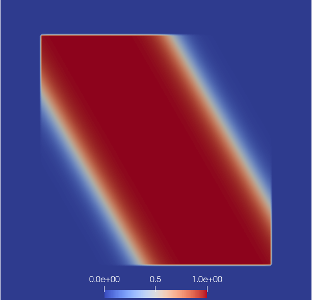
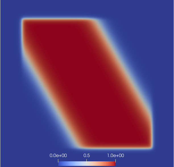
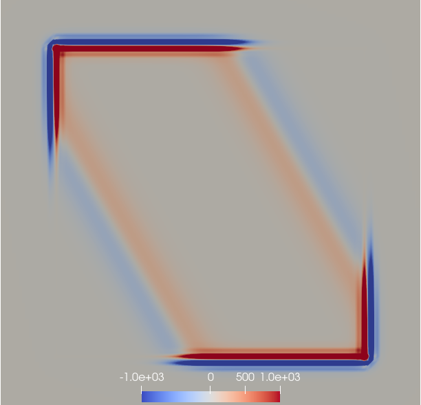
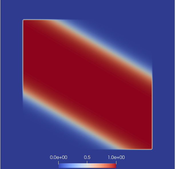
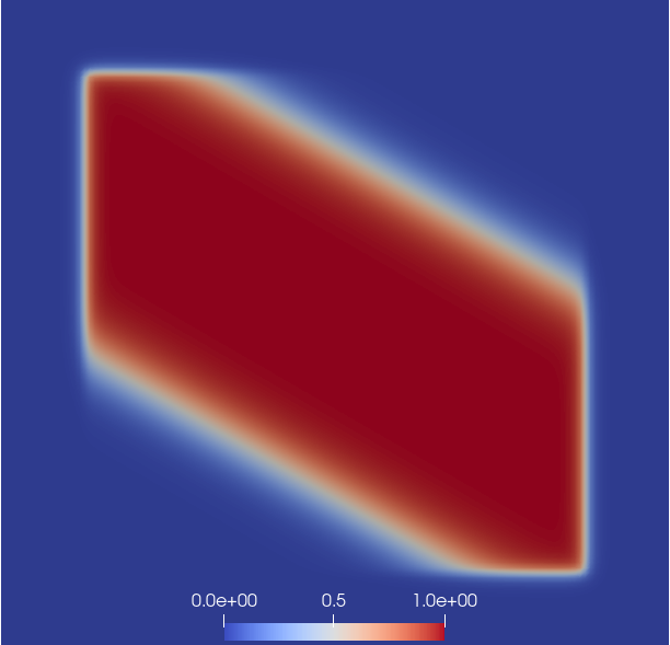
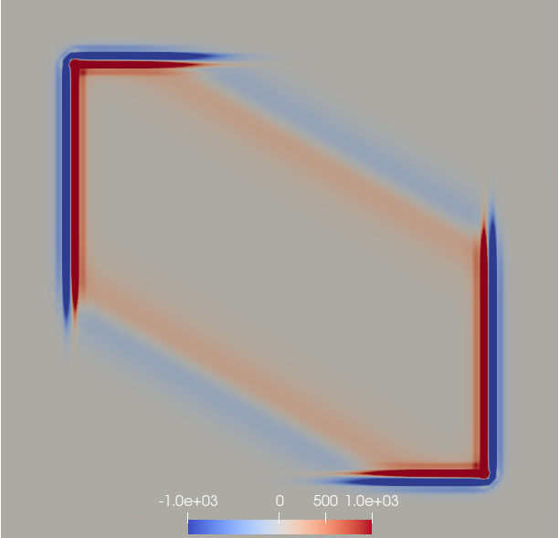
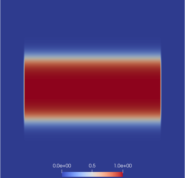
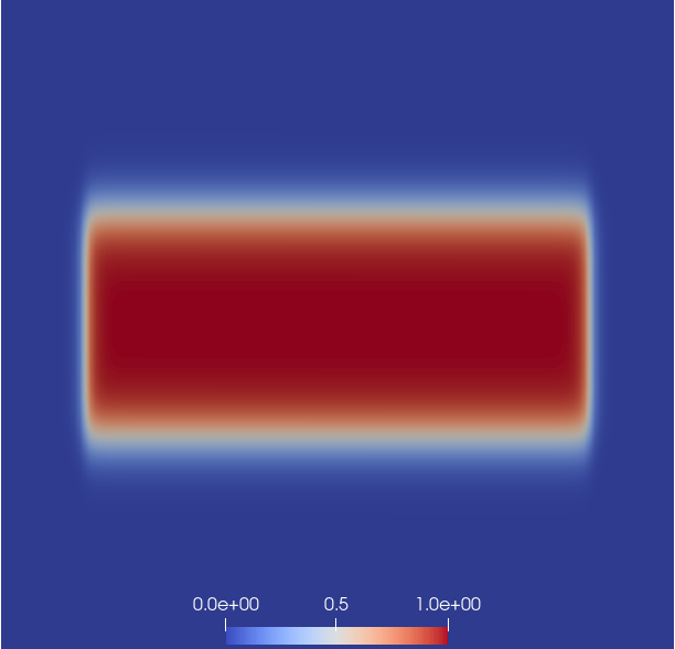
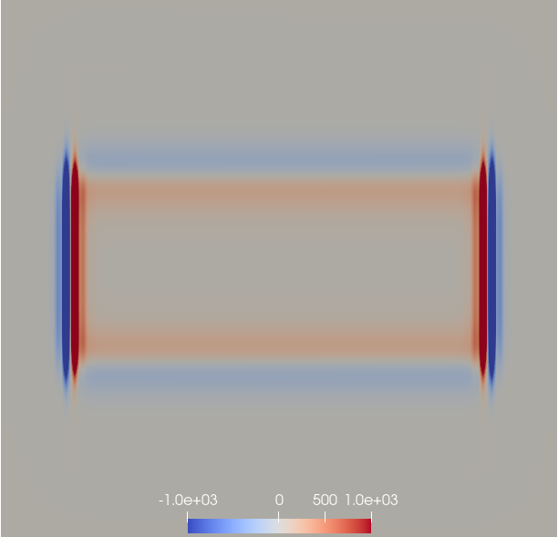
Figure 1: Simulation results for the nonlinear turning wave example with $n_{t}=n_{x}=128$. Target (left), state (middle), and control (right) at $t=0.25$ (top), $t=0.5$ (middle), and $t=0.75$ (bottom).

In Figure 2 we finally summarize the computing times for all examples, confirming, up to logarithmic factors, optimal complexity in all cases.

Figure 2: Simulation times for all cases.

6 Conclusions

In this paper we have formulated and analyzed a new approach to solve distributed optimal control problems subject to the heat equation as a minimization problem with respect to the state in the anisotropic Sobolev space $H^{1,1/2}_{0;0,}(Q)$ where we also present an efficient approach of optimal complexity to evaluate the norm in $H^{1/2}_{0,}(0,T;L^{2}(\Omega))$. While the application of the fast sine transformation requires a space-time tensor product mesh which is uniform in time, we can use either tensor-product or simplicial meshes in space. In order to handle adaptive meshes in space, and as in [15] for the elliptic case, we can introduce a variable energy regularization in space, i.e., instead of (3.5) we can minimize the reduced cost functional

$$\widetilde{\mathcal{J}}(u_{\varrho})=\frac{1}{2}\,\|u_{\varrho}-\overline{u}\|^{2}_{L^{2}(Q)}+\frac{1}{2}\,\varrho_{t}\,\langle\partial_{t}u_{\varrho},{\mathcal{H}}_{T}u_{\varrho}\rangle_{Q}+\frac{1}{2}\,\int_{0}^{T}\int_{\Omega}\varrho_{x}(x)\,|\nabla_{x}u_{\varrho}(x,t)|^{2}\,dx\,dt,$$

where $\varrho_{t}$ is a constant to be chosen accordingly, and $\varrho_{x}(x)=h_{x,\ell}^{2}$ for $x\in\tau_{\ell}\subset\Omega$. The results of such an approach will be published elsewhere.

The focus of this paper was on the efficient solution of the optimal control problem without additional constraints neither on the state, nor on the control. But as in [10] we can handle both state and control constraints which the lead to variational inequalities to be solved by some iterative procedure, and which again requires an efficient handling of all matrices as described in this paper. Related results of these extensions will be published elsewhere.

It is without saying, that the proposed approach is also of interest to other optimal control and inverse problems subject to parabolic evolution equations, including nonlinear problems.

References

[1]
S. C. Brenner, J. Gedicke, L.–Y. Sung:
A symmetric interior penalty method for an elliptic distributed optimal
control problem with pointwise state constraints.
Comput. Methods. Appl. Math. 23 (2023) 565–589.
[2]
E. Casas: A review on sparse solutions in optimal control of partial
differential equations. SeMA 74 (2017) 319–344.
[3]
E. Casas, F. Kruse, K. Kunisch: Optimal control of semilinear parabolic
equations by BV-functions. SIAM J. Control Optim. 55 (2017) 1752–1788.
[4]
E. Casas, K. Kunisch: Parabolic control problems in space-time measure
spaces. ESAIM Control Optim. Calc. Var. 22 (2016) 355–370.
[5]
E. Casas, R. Herzog, G. Wachsmuth: Analysis of spatio-temporally sparse
optimal control problems of semilinear parabolic equations.
ESAIM Control Optim. Calc. Var. 23 (2017) 263–295.
[6]
E. Casas, C. Ryll, F. Tröltzsch: Sparse optimal control of the
Schlögl and FitzHugh–Nagumo systems.
Comput. Methods Appl. Math. 13 (2013) 415–442.
[7]
P. Deuflhard, A. Schiela, M. Weiser: Mathematical cancer therapy planning in
deep regional hyperthermia. Acta Numerica 21 (2012) 307–378.
[8]
M. Frigo, S. G. Johnson: The design and implementation of FFTW3.
Proceedings of the IEEE 93 (2005) 216–231.
[9]
P. Gangl, S. Köthe, C. Mellak, A. Cesarano, A. Mütze: Multi-objective
free-form shape optimization of a synchronous reluctance machine.
COMPEL 41 (2022) 1849–1864.
[10]
P. Gangl, R. Löscher, O. Steinbach: Regularization and finite element
error estimates for elliptic distributed optimal control problems with
energy regularization and state or control constraints.
arXiv:2306.15316, 2023.
[11]
M. Gunzburger, A. Kunoth: Space-time adaptive wavelet methods for
optimal control problems constrained by parabolic evolution equations.
SIAM J. Control Optim. 49 (2011) 1150–1170.
[12]
R. Herzog, G. Stadler, G. Wachsmuth: Directional sparsity in optimal
control of partial differential equations.
SIAM J. Control Optim. 50 (2012) 943–963.
[13]
R. Herzog, M. Heinkenschloss, D. Kalise, G. Stadler, E.Trélat (eds.):
Optimization and Control for Partial Differential Equations, vol. 29 of
Radon Series on Computational and Applied Mathematics, de Gruyter, 2022.
[14]
K. Kunisch, K. Pieper, B. Vexler: Measure valued directional sparsity
for parabolic optimal control problems.
SIAM J. Control Optim. 52 (2014) 3078–3108.
[15]
U. Langer, R. Löscher, O. Steinbach, H. Yang:
An adaptive finite element method for distributed elliptic optimal
control problems with variable energy regularization.
arXiv:2209.08811, 2022.
[16]
U. Langer, R. Löscher, O. Steinbach, H. Yang:
Robust finite element discretization and solvers for distributed
elliptic optimal control problems.
Comput. Methods Appl. Math. 23 (2023) 989–1005.
[17]
U. Langer, R. Löscher, O. Steinbach, H. Yang: Mass-lumping
discretization and solvers for elliptic optimal control problems.
arXiv:2304.14664, 2023.
[18]
U. Langer, O. Steinbach, F. Tröltzsch, H. Yang:
Unstructured space–time finite element methods for optimal control
of parabolic equations. SIAM J. Sci. Comput. 43 (2021) A744–A771.
[19]
U. Langer, O. Steinbach, F. Tröltzsch, H. Yang:
Space-time finite element discretization of parabolic optimal
control problems with energy regularization.
SIAM J. Numer. Anal. 59 (2021) 675–695.
[20]
U. Langer, O. Steinbach, F. Tröltzsch, H. Yang: Unstructured space-time
finite element methods for optimal sparse control of parabolic equations.
In: Optimization and Control for Partial Differential Equations.
Uncertainty quantification, open and closed-loop control, and shape
optimization. (R. Herzog, M. Heinkenschloss, D. Kalise, G. Stadler,
E. Trelat eds.). Radon Series on Computational and Applied Mathematics,
vol. 29, de Gruyter, Berlin, pp. 167–188, 2022.
[21]
U. Langer, O. Steinbach, H. Yang:
Robust space-time finite element methods for parabolic