Axion star condensation
around primordial black holes
and microlensing limits

Abstract

We present novel findings concerning the parameter space of axion stars, extended object forming in dense dark matter environments through gravitational condensation. We emphasize their formation within the dense minihalos that potentially surround primordial black holes and in axion miniclusters. Our study investigates the relation between the radius and mass of an axion star in these dense surroundings, revealing distinct morphological characteristics compared to isolated scenarios. We explore the implications of these results when applied to gravitational microlensing from extended objects and gravitational wave detection from compact binaries, leading to insights on the observational constraints from such “halo” axion stars. We provide a constraint on the fraction of the galactic population of axion stars from their contribution to the microlensing events from the EROS-2 survey, using the numerical resolution of the Schrödinger-Poisson equation.

1 Introduction

Astrophysical and cosmological observations suggest that approximately 27% of the energy content of the universe resides in dark matter (DM) [1, 2, 3, 4]. This picture agrees with structure formation [5], the gravitational lensing of distant objects [6, 7], and the rotation curves of galaxies [8]. The gravitational effects of DM are undeniable, including its importance in the cosmological history. Yet, its elusive non-gravitational interactions have remained beyond the reach of traditional observational methods. For this, the nature of DM is currently a debated subject, with various theories proposing a particle candidate that stems beyond the Standard Model of particles (SM).

One compelling DM candidate is the QCD axion [9, 10], a hypothetical particle predicted within the solution to the strong-CP puzzle proposed by Peccei and Quinn (PQ) [11]. The QCD axion’s origin lies within the framework of the PQ mechanism, which introduces a new global symmetry to QCD, thereby dynamically suppressing CP-violating terms. The breaking of this symmetry at high energies gives rise to a pseudo Nambu-Goldstone boson, the axion, endowed with a mass that is inversely proportional to the energy scale at which the symmetry breaking occurs. For recent reviews see refs. [12, 13]. Remarkably, the QCD axion might serve both as a solution to the strong-CP puzzle while concurrently offering a plausible explanation for the cosmic DM budget. In fact, the particle’s lifetime would exceed the age of the Universe, behaving as a pressureless non-interacting fluid on galactic or cosmological scales [14, 15, 16].

The properties of the primordial distribution of the axion field are affected by its cosmological history, with large inhomogeneities developing in the scenario where the PQ symmetry breaks after inflation [17, 18, 19, 20]. This has been recently confirmed in numerical simulations of the axion field evolution [21, 22, 23, 24, 25, 26, 27, 28]. Owing to this clumpy spatial distribution, it is expected for many regions to undergo gravitational collapse as fluctuations become non-linear, leading to axion miniclusters [29, 30, 31, 32, 33]. These objects are expected to form if the PQ symmetry breaks after inflation, as shown in both theoretical setups [34, 35] and numerical simulations [36, 37, 38, 35]. These dense objects might even survive tidal disruption to date and be part of the galactic halos [39, 40], leading to indirect evidences such as microlensing [41, 42, 43, 44] and particle conversion in strong magnetic fields [45, 46].

These inhomogeneities could be expected even in the complementary scenario where the PQ symmetry breaks before or during inflation, through the formation of axionic “dark minihalos” around primordial black holes (PBHs) [47]. The formation of these structures could proceed even in the absence of primordial DM seeds. The importance of this remark stems in the fact that PBHs could have formed at different mass scales and across various cosmological scenarios, possibly independently of the history of the axion field.

In addition to its role as a potential DM constituent, the QCD axion has also been implicated in the formation of axion stars, time-periodic solutions of the Einstein-Klein-Gordon equations [48, 49]. Axion stars are hypothesized to arise from the gravitational collapse of axion clouds, wherein the gravitational collapse is counteracted by the pressure term arising from Heisenberg’s uncertainty principle, thus leading to a stable, gravitationally-bound configuration. For this, axion stars exhibit intriguing characteristics, including a Bose-Einstein condensate-like behavior, wherein vast numbers of axions occupy the lowest energy state, manifesting macroscopic quantum phenomena on macroscopic scales. Axion stars might have formed inside the dense environment of axion miniclusters or the dense PBH minihalos [50, 51, 47]. The process of nucleation has been assessed numerically with the corresponding gravitational timescale being under control from the theory viewpoint. Axion stars have been extensively studied as isolated objects in the vacuum, in the so-called “dilute” regime [48, 52, 53, 54, 55].

Several techniques employed in the search for diffuse dark clumps in galaxies include parametric-induced explosions of axion stars into photons [56, 57, 58] or relativistic axions [59, 50, 60], the gravitational wave [61] and photon resonances [56] from post-mergers, and gravitational microlensing. This latter method is characterized by the amplification of brightness in background source stars as clumps pass near the line of sight. Notably, the abundances of massive compact halos and PBHs undergo stringent scrutiny through gravitational lensing observations. Surveys such as the Expérience de Recherche d’Objets Sombres (EROS) [62, 63], the MAssive Compact Halo Objects (MACHO) [64], the Optical Gravitational Lensing Experiment (OGLE) [65, 66], and the Microlensing Observations in Astrophysics (MOA) [67] collaborations play pivotal roles in these constraint efforts.

Unlike PBHs, DM clumps in the form of dark minihalos and axion stars possess internal structures that generally make them unsuitable for a treatment in terms of point-like massive objects, when dealing with microlensing events. Consequently, to accurately assess the microlensing constraints on axion clumps, finite lens size effects have to be accounted for. Numerous investigations have explored microlensing events caused by astrophysical objects with finite extents, including boson stars and self-similar subhalos [43, 42, 68]. Additionally, the gravitational lensing phenomenon associated with axion miniclusters has been explored in previous research [69, 41, 70].

In this work, we consider the formation of an axion star inside a dark minihalo surrounding a PBH and in axion miniclusters. The density profile of the minihalo is predicted from the spherical collapse and accretion of pressureless DM. The conditions imposed in this dense environment modify the morphology of the axion star, leading to a different relation between its mass and radius compared to the case of a dilute star. We call these objects “halo” axion stars. We consider light PBHs in the asteroid mass window, where axion stars of comparable magnitude in mass can form through gravitational condensation. These objects lead to interesting phenomenology such as microlensing from extended objects and an enhanced gravitational wave signal with respect to dilute axion stars in binary configurations. This provides a complementary route to search for both a PBH population and the DM component in the form of a light boson. One of the primary objectives of this study is to derive microlensing constraints from surveys targeting axion clumps. Since the model predicts an extended lens in the form of axion stars and dark minihalos, we constrain the fraction of these objects with microlensing using the data from the EROS-2 survey [63]. We use the full numerical solution of the Schrödinger-Poisson system for modeling the profile of the axion star.

The paper is organized as follows. In section 2 we introduce the methods used in our computations. Results are drawn in section 3 and discussed in section 4. We comment on the outcome and future directions in the conclusions of section 5. We set $\hbar=c=1$ throughout the paper.

2 Methods

2.1 Properties of the dark minihalo

The process of modeling DM accretion around one PBH has been tackled both analytically and through N-body simulations. Here, PBHs constitute only a very small fraction of the DM, with the axion contributing to the bulk DM budget. Some of the axion DM accumulates around the PBH, forming a dark halo [71, 72, 73, 74, 75]. This occurs in the early Universe through the joint action of the gravitational attraction from rogue PBHs and the Hubble expansion, which leads to the acceleration of a DM shell of radius $r$ around an isolated PBH of mass $M_{\rm PBH}$ as

$$\frac{{\rm d}^{2}r}{{\rm d}t^{2}}=-\frac{r_{g}}{r^{2}}+\left(\dot{H}+H^{2}\right)r\,,$$ (2.1)

where $r_{g}=GM_{\rm PBH}$ is the gravitational radius of the PBH, $H$ is the Hubble rate, and $\dot{H}$ its variation with respect to time $t$. By the time of matter-radiation equality (“eq”), the dark minihalo around a PBH of mass $M_{\rm PBH}$ possesses a spiky distribution with density profile

$$\rho_{\rm spike}(r)=\frac{\rho_{\rm eq}}{2}\,\left(\frac{r_{\rm ta}(t_{\rm eq})}{r}\right)^{9/4}\,,$$ (2.2)

where $\rho_{\rm eq}$ is the density at redshift $z_{\rm eq}\approx 3400$ and the time $t_{\rm eq}$ is fixed through the expression

$$t_{\rm eq}=\left(\frac{3}{32\pi G\rho_{\rm eq}}\right)^{1/2}\,.$$ (2.3)

The turn-around radius $r_{\rm ta}$ defines the region within which the gravitational influence of the PBH overcomes cosmic expansion and corresponds to setting $\dot{r}=0$ in eq. (2.1), or [74]

$$r_{\rm ta}(t)\approx(2r_{g}\,t^{2})^{1/3}\,.$$ (2.4)

In this setup, the expression in eq. (2.2) holds for $r<r_{\rm ta}(t_{\rm eq})$ at time $t_{\rm eq}$. For example, a PBH of mass $M_{\rm PBH}=10^{-13}\,M_{\odot}$ has $r_{\rm ta}(t_{\rm eq})\approx 0.26$ au.

The dark minihalo radius keeps growing through accretion, as expected both from simulations [78, 79] as well as calculations of the virial mass and radius [72]. The halo radius can be fixed by setting the cutoff at the halo overdensity $\delta_{H}=1$,

$$R_{\rm halo}(z)\approx\,r_{\rm ta}(t_{\rm eq})\,\left(\frac{1+z_{\rm eq}}{1+z}\right)^{4/3}\,.$$ (2.5)

At any redshift, the mass of the dark minihalo can be express by integrating the density profile to the radius $R_{\rm halo}(z)$,

$$M_{\rm halo}=\int_{0}^{R_{\rm halo}}{\rm d}r\,4\pi r^{2}\rho_{\rm spike}(r)=\frac{8\pi}{3}\rho_{\rm eq}r^{3}_{\rm ta}(t_{\rm eq})\left(\frac{R_{\rm halo}(z)}{r_{\rm ta}(t_{\rm eq})}\right)^{3/4}\approx\frac{8}{9}M_{\rm PBH}\,\left(\frac{1+z_{\rm eq}}{1+z}\right)\,,$$ (2.6)

where the additional factor 8/9 accounts for the evolution in the matter-dominated era. This result, previously obtained with other methods [78, 79], holds down to the redshift $z_{\rm gal}\sim 30$ where growth typically stops due to tidal interactions. At any time, the mass enclosed within the radius $r$ and the corresponding virial velocity $v$ can be obtained from integrating to the radius $r<R_{\rm halo}\equiv R_{\rm halo}(z_{\rm gal})$ within the DM halo,

$$M_{\rm encl}(r) = M_{\rm PBH}+M_{\rm halo}\,\left(\frac{r}{R_{\rm halo}}\right)^{3/4}\,,$$ (2.7)

$$v^{2} = \frac{GM_{\rm encl}(r)}{r}\,.$$ (2.8)

2.2 Axion star nucleation

The results of the previous section are obtained for a pressureless fluid and thus apply to different models of cold DM. We now specialize the discussion to the QCD axion, where particle-particle interactions can lead to an enhancement of the quantum properties of these light bosons through gravitational condensation.

The condensation of axion stars inside miniclusters and dark minihalos has been studied in the literature through numerical simulations, accounting for both self-gravitating light particles [80] and with the inclusion of self-interactions [81, 82, 83, 84, 85, 86]. If gravity provides the dominant contribution to the particle interaction, the time scale of the Bose star formation process is [80]

$$\tau_{\rm gr}\approx\frac{\sqrt{2}}{12\pi^{3}}\frac{m_{a}v^{6}}{G^{2}n^{2}\Lambda}\,,$$ (2.9)

where $n$ is the DM number density and the Coulomb logarithm $\Lambda=\ln(m_{a}vR_{\rm halo})$ accounts for the scale of the system $R_{\rm halo}$. While the quantities $v$ and $n$ entering eq. (2.9) involve local properties of the halo, the size of the halo only appears in the logarithmic correction, so that the structure of the halo does not greatly affect the outcome of the computation.

We demand two conditions that should be satisfied inside the dark minihalo for the formation of an axion star to take place. First of all, the halo has to be sufficiently large to host the de Broglie wavelength of the axion,

$$m_{a}\,v\,R_{\rm halo}\gg 1\,,$$ (2.10)

and the kinetic regime condition should occur sufficiently fast [80]

$$m_{a}\,v^{2}\,\tau_{\rm gr}\gg 1\,.$$ (2.11)

We also demand that the axion star actually forms on a timescale shorter than the age of the Universe at redshift $z$,

$$\Gamma_{\rm kin}(r)\gtrsim\left(\frac{t_{0}}{(1+z)^{3/2}}\right)^{-1}\,,$$ (2.12)

where the kinetic relaxation rate is [47]

$$\Gamma_{\rm kin}(z)\approx n\,\sigma_{\rm gr}\,v\,N\approx n^{2}\,\frac{48\pi^{2}G^{2}\Lambda}{m_{a}\,v^{6}}\,.$$ (2.13)

Setting $n=\rho_{\rm spike}(r)/m_{a}$, eq. (2.12) at a given redshift $z$ can be used to obtain the critical radius $R_{\rm crit}$ within which at least one axion star forms inside the dark minihalo,

$$R_{\rm crit}=r_{\rm ta}\left(\frac{81\Lambda}{128\pi G\rho_{\rm eq}r^{6}_{\rm ta}(t_{\rm eq})m_{a}^{3}}\frac{t_{0}}{(1+z)^{3/2}}\right)^{4/15}\,,$$ (2.14)

with the additional requirement $R_{\rm crit}<R_{\rm halo}(z)$.

Under the condition for the nucleation outlined above, we proceed to understand the properties of nonrelativistic axion stars, solitonic solutions of the Schrödinger-Poisson equation [48]

$$\nabla^{2}\phi =4\pi G\left(\rho+M_{\rm PBH}\delta^{(3)}({\bf r})\right)\,,$$ (2.15)

$$\epsilon\psi =-\frac{1}{2m}\nabla^{2}\psi+\left(\frac{\lambda_{\Phi}}{8m^{2}}\psi^{*}\psi+m\phi\right)\psi\,.$$ (2.16)

Here, $\lambda_{\Phi}$ is the self-coupling constant, see eq. (A.9) in Appendix A, $\phi$ is the gravitational potential of the axion star and the PBH source, and the relation between energy density $\rho$ and $\psi$ is

$$m|\psi|^{2}=\rho\,.$$ (2.17)

Axion stars are expected to form in the central regions inside the dark minihalo surrounding a PBH and in axion miniclusters. If the nucleation occurs far from the center, the gravity potential of the PBH does not enter the Poisson eq. (2.15) but it would affect the structure of the axion star through tidal interactions [47]. The mechanism proceeds if the central density of the minihalo is sufficiently high for two-to-two processes to relax the energy of the axions in the inner core, leading to particle condensation [80, 81, 82, 83, 84, 85, 86]. For a halo of ultralight particles, numerical simulations predict the relation between the halo mass and the axion star mass as [87, 88]

$$M_{\rm AS}\approx 1.8\times 10^{-10}\,M_{\odot}\,\left(\frac{1+z}{1+z_{\rm eq}}\right)^{1/2}\,\left(\frac{\mu\rm eV}{m_{a}}\right)\,\left(\frac{M_{\rm halo}}{M_{\odot}}\right)^{1/3}\,.$$ (2.18)

Other simulations with N-bodies on the formation of a solitonic core in massive halos find similar results [89]. The profile of a solitonic core around a supermassive BH has also been studied numerically [90, 91]. Consistency demands that the mass of the axion star be $M_{\rm AS}<M_{\rm halo}$, leading to a fourth requirement that has to be satisfied for the formation of the star in the halo.

3 Results

3.1 Dark minihalo

We now specialize these requirements to the dark minihalo discussed previously. Setting $\Lambda\approx 7$, combining the kinetic condition in eqs. (2.10), (2.11), (2.12) and (2.18) gives

$$m_{a}vR_{\rm halo} \sim 500\left(\frac{m_{a}}{10^{-5}{\rm\,eV}}\right)\left(\frac{10^{3}}{1+z}\right)^{\frac{7}{6}}\left(\frac{M_{\rm PBH}}{10^{-13}M_{\odot}}\right)^{\frac{2}{3}}\,,$$ (3.1)

$$(m_{a}v^{2}\tau_{\rm gr})^{1/4} \sim 400\left(\frac{m_{a}}{10^{-5}{\rm\,eV}}\right)\left(\frac{10^{3}}{1+z}\right)^{\frac{7}{6}}\left(\frac{M_{\rm PBH}}{10^{-13}M_{\odot}}\right)^{\frac{2}{3}}\,,$$ (3.2)

$$\left(\frac{R_{\rm halo}}{R_{\rm crit}}\right)^{\frac{5}{4}} \sim 500\,\left(\frac{m_{a}}{10^{-5}{\rm\,eV}}\right)\left(\frac{10^{3}}{1+z}\right)^{\frac{7}{6}}\left(\frac{M_{\rm PBH}}{10^{-13}M_{\odot}}\right)^{\frac{2}{3}}\,,$$ (3.3)

$$\frac{M_{\rm halo}}{M_{\rm AS}} \sim 500\,\left(\frac{m_{a}}{10^{-5}{\rm\,eV}}\right)\left(\frac{10^{3}}{1+z}\right)^{\frac{7}{6}}\left(\frac{M_{\rm PBH}}{10^{-13}M_{\odot}}\right)^{\frac{2}{3}}\,.$$ (3.4)

Surprisingly, all four of the expressions above lead to the same functional dependence in terms of redshift $z$, axion mass $m_{a}$, and halo mass. This has not been anticipated before, since eq. (2.18) has been derived from the numerical properties of the cosmological simulation and is thus independent from the considerations that lead to the first three expressions.

We impose that all four quantities above exceed unity, to satisfy the conditions for the formation and the stability of the axion star. When plotting these constraints on the parameter space $\left(M_{\rm halo},m_{a}\right)$, the four expressions lead to parallel lines, with the latter coming from the requirement $M_{\rm AS}<M_{\rm halo}$ yielding the slightly most stringent bound. Figure 1 summarizes the results obtained. The density plot accounts for the axion star mass in eq. (2.18) as a function of the halo mass (horizontal axis) and the axion mass (vertical axis). Also shown is the bound derived from demanding that the axion star forms by $z\approx 30$, with a halo that is massive enough to contain it as $M_{\rm AS}<M_{\rm halo}$, as expressed in eq. (3.4). Also shown in the plot are the regions favored by some recent simulations of the QCD axion mass from cosmic string simulations, including “Saikawa24” [28] predicting $m_{a}\in[95\textrm{-}450]\,\mu$eV (area within the red dashed lines), “Buschmann21” [26] predicting $m_{a}\in[40\textrm{-}180]\,\mu$eV (area within the green dot-dashed lines), and “Gorghetto20” [25] predicting $m_{a}>500\,\mu$eV (area above the blue dotted line). The region labeled “Arvanitaki15” marks the exclusion of the QCD axion in the mass range $m_{a}\in[6\textrm{-}200]\times 10^{-13}\,$eV, obtained from stellar black hole spin measurements [92]. Finally, the region to the right of the vertical dashed line labeled “Lensing” can be probed by gravitational microlensing of the dark minihalos in the Galaxy, see section 4 below. This result extends the findings in ref. [47] to include the bounds presented in eqs. (3.1)-(3.4) in a systematic way, as well as providing a link between the parameter space and the mass of the axion star through eq. (2.18).

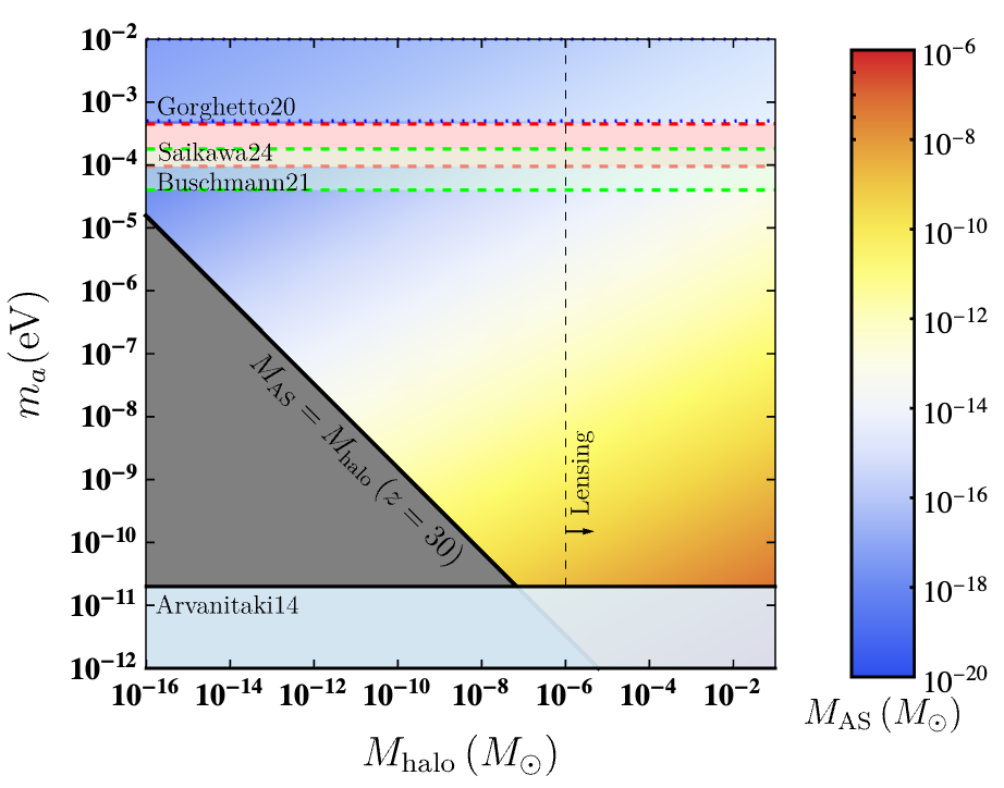
Figure 1: The mass of the axion star as a function of the halo mass (horizontal axis) and the QCD axion mass (vertical axis). The color map shows the mass of the corresponding axion star for values of the pair $\left(M_{\rm halo},m_{a}\right)$ at $z=30$. The region below the black solid line shows the constrain from the mass ratio between axion stars and the axion halo given in eq. (3.4). Also shown is the reach from gravitational microlensing (right of the vertical dashed line), the region excluded by stellar black hole spin measurements (light blue), and the prediction of the QCD axion mass from numerical simulations (see text for details).

We consider now axion stars orbiting a PBH of mass $M_{\rm PBH}\gg M_{\rm AS}$ and nucleating close to the center of the distribution. We generally expect that these axion stars possess an inner structure which is dominated by the gravitational potential of the PBH itself. In fact, when the self-gravity potential of the axion star density can be neglected, eq. (2.16) resembles a gravitational atom, with ground state

$$\psi(r)=\alpha^{3}\,\left(\frac{M_{\rm AS}}{\pi\,r_{g}^{3}}\right)^{1/2}\,\exp\left(-\alpha^{2}r/r_{g}\right)\,,$$ (3.5)

where $\alpha=r_{g}m_{a}\equiv GM_{\rm PBH}m_{a}$ measures the gravitational coupling of the axion in the gravitational field of the PBH. The corresponding energy of the ground state is $E_{0}=-\alpha^{2}m/2$, and the radius containing 90% of the mass is

$$R_{\rm AS}\approx 2.66\,r_{g}/\alpha^{2}\,.$$ (3.6)

For the axion star radius to be relevant in this context, we generally expect that it encompasses the corresponding Schwarzschild radius of the PBH, $R_{\rm AS}\gtrsim 2r_{g}$, or $\alpha\lesssim 1$. Setting $m_{a}\gtrsim 10^{-9}\,$eV for the QCD axion leads to $M_{\rm PBH}\lesssim 0.1\,M_{\odot}$.

3.2 Axion minicluster

We compare these results with the shape and mass window for the axion star formed inside an axion minicluster (“amc”), for which the density undergoing spherical collapse reaches the value [32]

$$\rho_{\rm amc}(\delta)\approx 140\,\delta^{3}\,(1+\delta)\,\rho_{\rm eq}\,,$$ (3.7)

where the overdensity parameter $\delta$ models the excess density in the minicluster with respect to the background. The radius of the minicluster $R_{\rm amc}$ is then fixed in terms of $\delta$ and the halo mass $M_{\rm halo}$, so that eq. (3.7) gives the average density of the minicluster. With this choice, the inner density profile is found as [41, 93]

$$\rho(r)=\frac{1}{4}\,\rho_{\rm amc}(\delta)\,\left(\frac{R_{\rm amc}}{r}\right)^{9/4}\,,$$ (3.8)

for $r<R_{\rm amc}$, and zero otherwise. For this, we wish to test the relation between the axion star mass $M_{\rm AS}$ and the halo mass $M_{\rm halo}$ given in eq. (2.18) by solving the Schrödinger-Poisson system of eqs. (2.15)-(2.16) to obtain the mass of the star. More in detail, we proceed with the resolution using the formulas outlined in Appendix A which, following closely ref. [52], consists in rewriting the set of eqs. (2.15)-(2.16) into a dimensionless form that does not depend on the QCD axion mass or the energy scale. Once the solution for the density profile is obtained, the radius of the axion star is then fixed through a prescription that involves the total mass of the star [94, 95]. Contrary to the fermion star, the boson star does not have a defined radius which needs to be specified by some additional condition. Previous work considered the radius containing a percentage of the mass of the star [52, 54]. Here, we define the radius of the dilute axion star as the radius enclosing 90% of its total mass, or

$$R_{\rm AS}\approx\frac{6.84}{G\,m_{a}^{2}\,M_{\rm AS}}\,,$$ (3.9)

where the details to fix the numerical value in the numerator are discussed in Appendix A. For a given $m_{a}$, we obtain a family of solutions in terms of a set of masses and radii ($M_{\rm AS},R_{\rm AS}$), depending on the central density of the axion star. The density of the star decreases with decreasing mass, so that a lower bound on the axion star mass comes from demanding that the star fits inside the minihalo, $R_{\rm AS}<r_{\rm ta}(t_{\rm eq})$. This requirement assures that the density of the star at the stellar radius does not fall below the average DM density at the time of formation. On the other end, an upper bound exists because of the existence of self-interactions that destabilize the stellar equilibrium, and leads to the request (see e.g. ref. [54])

$$M_{\rm AS}\lesssim 3\times 10^{-20}\,M_{\odot}\,({\rm eV}/m_{a})^{2}\,,$$ (3.10)

where the expression above implicitly assumes the ratio of the up and down quark masses $m_{u}/m_{d}=0.48$.

We compare the results obtained for a pristine “dilute” axion star formed in the vacuum with a star formed in the dense environment of a minicluster considered here. For such a “halo” axion star, we impose a different cutoff for its radius by considering the density of the surrounding environment. Assuming that the star forms at the center of the minicluster, the radius is obtained from the condition

$$\rho(R_{\rm AS})=\frac{1}{4}\,\rho_{\rm amc}(\delta)\,\left(\frac{R_{\rm amc}}{R_{\rm AS}}\right)^{9/4}\,.$$ (3.11)

The profiles for a dilute and a halo axion star are compared in figure 2 for the QCD axion mass $m_{a}=100\,\mu$eV and an axion minicluster of mass $M_{\rm amc}=10^{-11}\,M_{\odot}$ with overdensity parameter $\delta=1$, for different values of the axion star. This corresponds to the radius $R_{\rm amc}\approx 5.4\times 10^{7}\,$km. The condensation at the core of the minicluster modifies the density profile and leads to a flat plateau instead of the spike predicted by the pressureless DM. This corresponds to the general behaviour seen in the numerical simulations that deal with structure formations with ultralight axions, although the length scales in play here are astronomical instead of galactic.

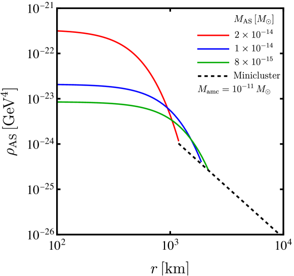
Figure 2: The density profile of various axion stars with different mass, hosted inside a minicluster of mass $M_{\rm amc}=10^{-11}\,M_{\odot}$ with overdensity parameter $\delta=1$. Specifically, we have fixed the masses $M_{\rm AS}=2\times 10^{-14}\,M_{\odot}$ (red), $M_{\rm AS}=1\times 10^{-14}\,M_{\odot}$ (blue), and $M_{\rm AS}=8\times 10^{-15}\,M_{\odot}$ (green). The mass of the QCD axion is fixed as $m_{a}=100\,\mu$eV.

We now turn to fixing the radius of the axion star by means of the condition in eq. (3.11). The prescription leads to a non-trivial behaviour for mass-radius relation with respect to what is found in eq. (3.9). This is shown in figure 3 for the axion stars forming inside an axion minicluster of mass $M_{\rm amc}=10^{-12}\,M_{\odot}$ (blue) or $M_{\rm amc}=10^{-11}\,M_{\odot}$ (red), compared with the predictions from eq. (3.9) with $m_{a}=100\,\mu$eV. A maximum radius is expected for the axion star, above which the condition for the condensation timescale in eq. (2.9) would not be satisfied within the volume of the star. The prediction shown can be tested in simulations that follow the condensation of the axion star system as in refs. [80, 85], however to date no study at various axion star masses exists.

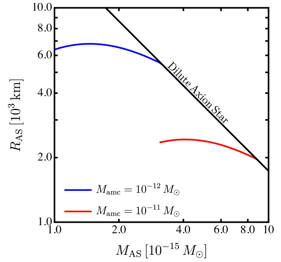
Figure 3: Mass-radius relation for different models of non-relativistic axion stars. We fix $m_{a}=100\,\mu$eV. The results show the “dilute” branch (black dashed line), the “halo” axion star branch with $M_{\rm amc}=10^{-12}\,M_{\odot}$ (blue line), and $M_{\rm amc}=10^{-11}\,M_{\odot}$ (red line), both of overdensity parameter $\delta=1$.

One consequence of this finding is the impact on the mass distribution of axion stars. Assessing the halo mass function for axion miniclusters is a primary goal to correctly predict the outcome from indirect phenomena such as the gravitational microlensing from dense objects [41]. The halo mass function has been derived numerically in previous studies using hierarchical merging, revealing that such a function follows a steep power-law distribution [96, 36]. However, for relatively low masses of the miniclusters the gravitational condensation into an axion star has to be accounted for since, for such low-mass clusters, the timescale in eq. (2.9) would lead to the formation of a large soliton. See e.g. ref. [39] for a discussion of this effect in terms of the tidal stripping of miniclusters from nearby stars. The results in figure 3 show that, on top of these considerations, the deviation of the axion star from the dilute regime and the appearance of a configuration with a maximum radius would also contribute to modifying the results obtained thus far, further motivating for a numerical investigation of this physical system in the coming future.

4 Discussion

4.1 Gravitational wave signals

Axion stars are compact object whose inspiral in compact binaries could lead to a gravitational wave (GW) signal that is potentially detectable [97, 98, 99, 100]. We first discuss the expected signal in GWs from halo axion stars forming in the presence of a hosting PBH, as these objects could result to be more compact than their dilute axion star counterparts. Given a compact object of mass $M_{\rm obj}$ and radius $R_{\rm obj}$, the compactness is defined as $\mathrm{C}\equiv GM_{\rm obj}/R_{\rm obj}$. A dilute axion star would then possess a compactness

$$\mathrm{C}\equiv\frac{GM_{\rm AS}}{R_{\rm AS}}\approx 10^{-17}\,\left(\frac{M_{\rm AS}}{10^{-14}\,M_{\odot}}\right)^{2}\,\left(\frac{m_{a}}{100{\rm\,\mu eV}}\right)^{2}\,,$$ (4.1)

where Eq. (3.9) for the radius of the axion star has been used. Such a small value of C is not sufficient to make QCD axion stars with a sufficiently high compactness to deliver a significant output in GWs when combined into compact mergers. Simulations of axion star mergers and their signal forecast generally rely on axion-like particles as their fundamental fields.

For a halo axion star, the compactness could be enhanced by the additional gravitational field exerted by the PBH, leading to a radius which is as small as in Eq. (3.6). Moreover, the mass of the object is dominated by the central PBH. In this scenario, the compactness in Eq. (4.1) is enhanced by up to a factor $\sim(M_{\rm PBH}/M_{\rm AS})^{2}$, potentially providing to a large boost in the GW signal for compact binaries. The existence of these halo axion stars requires $GM_{\rm PBH}m_{a}\lesssim 1$ to avoid the Schwarzschild limit, suggesting that PBHs of mass

$$M_{\rm PBH}\lesssim 10^{-6}\,M_{\odot}\,\left(\frac{100{\rm\,\mu eV}}{m_{a}}\right)\,,$$ (4.2)

could potentially host these dense halo axion stars. The frequency of the GW resulting from the merging of two such identical object is estimated by Kepler’s third law as

$$f=\left(\frac{GM_{\rm tot}}{\pi^{2}\,\ell^{3}}\right)^{1/2}\,,$$ (4.3)

where $M_{\rm tot}$ is the total mass of the binary and $\ell$ is the semi-major axis of the orbit. The inspiral phase terminates at the innermost stable circular orbit (ISCO) which, for a binary each of compactness C, is $R_{\rm ISCO}=3GM_{\rm tot}/$C. This approach is observed in numerical analyses of NS orbits [101]. The corresponding frequency at ISCO is [102]

$$f_{\rm ISCO}=\frac{C^{\frac{3}{2}}}{3^{\frac{3}{2}}\pi\,GM_{\rm tot}}\approx 700{\rm\,Hz}\,\left(\frac{M_{\rm PBH}}{10^{-9}\,M_{\odot}}\right)^{2}\,\left(\frac{m_{a}}{100{\rm\,\mu eV}}\right)^{3}\,,$$ (4.4)

which is in range of the frequency band of LIGO. For comparison, the frequency at ISCO for a BH binary of similar mass would appear at a much higher band

$$f_{\rm ISCO}^{\rm PBH}\approx 2\times 10^{12}{\rm\,Hz}\,\left(\frac{10^{-9}\,M_{\odot}}{M_{\rm PBH}}\right)\,,$$ (4.5)

which in fact corresponds to the quest carried out in cavity searches, see e.g. refs. [103, 104]. For a compact object binary, the characteristic GW amplitude during the inspiral phase averaged over the orbital period in the quadrupole approximation is [105, 106]

$$h_{c}(f)=\sqrt{\frac{32}{5}}\,\frac{(G\,\mathcal{M})^{5/3}}{d}\,(\pi\,f)^{2/3}\,,$$ (4.6)

where $\mathcal{M}$ is the chirping mass and $d$ is the distance to the source. For this, both axion stars and PBH binary mergers do not provide with a strain $h_{c}(f)$ at the ISCO frequency sufficiently large to be detectable at present or near-future facilities. The object that emerges from the merging of two halo axion stars would be in a highly excited and non-spherical configuration, with the resulting axion star oscillating along two perpendicular axes and relaxing through the emission of scalar modes and GWs [107, 99, 61].

In eq. (4.4), the parameters have been chosen to match the frequency that is visible in LIGO. For higher values of the PBH mass the frequency would shift to higher frequencies potentially detectable in microwave cavities, phononic metamaterials [108], or enhanced magnetic conversion [109].

4.2 Gravitational microlensing

Axion stars can be searched by various indirect methods such as gravitational microlensing. The search for DM in the form of faint compact objects has been theorized in refs. [110] and sparked the active search through gravitational microlensing by several surveys [62, 63, 64, 65, 66, 67]. For this, the lensing events from axion and boson stars has been extensively considered in previous literature, see e.g. refs. [111, 41, 43, 42, 112, 70, 68].

We consider the lensing constraints on a population of dilute axion stars. We modify the results from previous work by considering the actual density distribution of the axion star inside the minihalo for a finite lens. This is achieved here by a numerical resolution of the density profile of the star using the Schrödinger-Poisson equation. We follow the standard notation in defining the observer-lens, lens-source, and observer-source distances as $D_{\rm L}$, $D_{\rm S}$, and $D_{\rm LS}\equiv D_{\rm S}-D_{\rm L}$, respectively, with the dimensionless ratio $x\equiv D_{\rm L}/D_{\rm S}$. Setting the angular radius of the Einstein ring $\theta_{\rm E}$, see eq. (B.4), gives the Einstein radius $R_{\rm E}\equiv D_{\rm L}\theta_{\rm E}$.

Using the axion stars formed in the dark minihalo as gravitational lenses with the profile obtained through eqs. (2.15)-(2.16), we derive the threshold impact parameter $u_{1.34}$ that leads to a total magnification $\mu_{\rm tot}\approx 1.34$, with the technical details given in Appendix B. Once the threshold impact parameter is provided, the total number of events is given in terms of the differential event rate as

$$N_{\rm events}=E\,\int_{0}^{1}{\rm d}x\int_{t_{\rm min}}^{t_{\rm max}}{\rm d}t_{\rm E}\,\frac{{\rm d}^{2}\Gamma}{{\rm d}x\,{\rm d}t_{\rm E}}\,,$$ (4.7)

where $E$ is the total exposure time of the survey. The event rate per microlensing source of mass $M_{\rm lens}$ is given by [113] (see also eq. (6) in ref. [43])

$$\frac{{\rm d}^{2}\Gamma}{{\rm d}x\,{\rm d}t_{\rm E}}=\epsilon(2t_{\rm E})\frac{2D_{\rm S}}{v_{0}^{2}M_{\rm lens}}\rho_{\rm lens}(x)v_{\rm E}^{4}(x)\,\exp\left({-v_{\rm E}^{2}(x)/v_{0}^{2}}\right)\,,$$ (4.8)

where $v_{0}\approx 220{\rm\,km\,s^{-1}}$ is the galactic circular velocity. Here, $t_{\rm E}$ is the time required to cross the Einstein ring radius and $v_{\rm E}(x)=u_{1.34}R_{\rm E}(x)/t_{\rm E}$ is the velocity of the crossing. Finally, $\epsilon(2t_{\rm E})$ is the efficiency of the instrument.

To obtain the bounds for the model we use the data from the EROS-2 survey [63] that includes observations of the Large Magellanic Cloud (LMC) and the Small Magellanic Cloud (SMC), to constrain the galactic fraction in axion stars. For this, the lensing event rate in eq. (4.8) is given in terms of the fraction of lensing objects $f_{\rm lens}$ as $\rho_{\rm lens}(r)=f_{\rm lens}\rho_{\rm DM}(r)$, where the DM distribution in the Milky Way halo is modeled with an isothermal profile as

$$\rho_{\rm DM}(r)=\frac{\rho_{s}}{1+(r/r_{s})^{2}}\,.$$ (4.9)

Here, the normalization constant is taken as $\rho_{s}=1.39{\rm\,GeV\,cm^{-3}}$ with the core radius $r_{s}=4.38\,$kpc. The radius $r$ is related to the fractional distance $x$ between the Earth and the lens as

$$r=\sqrt{r_{\odot}^{2}+x^{2}D_{S}^{2}-2x(1-x)\,r_{\odot}\,D_{S}\cos\ell\cos b}\,,$$ (4.10)

where $r_{\odot}=8.5\,$kpc and the distance to the source $D_{s}\simeq 50\,$kpc for LMC ($D_{s}\simeq 60\,$kpc for SMC). The longitude and latitude of the source in galactic coordinates are respectively $\ell=280.46^{\circ}$ and $b=-32.89^{\circ}$ for LMC ($\ell=302.81^{\circ}$ and $b=-44.33^{\circ}$ for SMC). In eq. (4.7), several parameters are tailored to the EROS-2 survey. The instrument efficiency is taken from ref. [63], the exposure time is $E\simeq 3.76\times 10^{7}$ years ($E\simeq 5.9\times 10^{6}$ years), the time range to cross the Einstein ring radius $t_{\rm E}\in[1,500]$, and the number of events is $N_{\rm events}=3.9$. Results for the allowed fraction of galactic dense object are shown in figure 4 for axion stars, which are generally too small to exhibit an extended distribution and thus appear in the survey as point-like objects.

Figure 4: Lensing constraints on the mass of the lens using the data from the EROS-2 survey for a population of axion stars.

5 Conclusions

In this paper, we have discussed the formation mechanism of a dark matter clump or dark “minihalo” around a primordial black hole (PBH) in the early Universe between the matter-radiation equality epoch at redshift $z_{\rm eq}$ and the onset of structure formation at $z_{\rm gal}\approx 30$. We have underlined the properties of such a dark minihalo, including its density profile, radius and mass $M_{\rm halo}$, according to previous studies. In the scenario where the dark matter is in the form of the QCD axion of mass $m_{a}$, we have considered the nucleation of axion stars inside an axion minicluster and a dark minihalo. We have extended the results obtained in previous literature to include the target of the axion star mass range that it available in the model, comparing it with current bounds from microlensing and theoretical findings for the axion mass. The results are shown in figure 1 for the axion star mass in terms of the parameter space ($M_{\rm halo},m_{\rm a}$).

By solving the Schrödinger-Poisson equation in the dark minihalo background, we have obtained the profile and the mass-radius relations for a soliton forming inside such an environment, here referred to as a “halo” axion star. We remarked that the properties of this object depend on the central PBH mass as depicted in figure 2. In particular, its non-trivial mass-radius relation $R_{\rm AS}=R_{\rm AS}(M_{\rm AS})$ differs from the power-law dependence $R_{\rm AS}\propto 1/M_{\rm AS}$ which has been historically observed for dilute axion stars in the vacuum. This has been explicitly shown in figure 3 for axion miniclusters of different masses. The existence of a maximum stellar radius impacts on the mass distribution of these objects and it could be the subject for future numerical investigations, such as a systematic study of the condensation of these objects in halos of different masses.

To corroborate the study on possible indirect imprints, we have assessed the effects of axion stars onto gravitational microlensing. We have improved over previous studies on the QCD axion by deriving the lensing power of an axion star from the numerical resolution of the Schrödinger-Poisson system, as detailed in appendix B. We have tested our results against the analysis by the EROS-2 survey of the microlensing events observing both LMC and SMC, leading to the bounds on the fraction of axion stars shown in figure 4. Future work in this direction will focus on the inclusion of the halo mass distribution into the lensing bounds. The potential appearance of gravitational waves from binary mergers of halo axion stars in future setups has also been discussed. While the compactness of these objects might not be sufficiently large for the GW strain from galactic binaries to be currently detectable, some configurations could appear in the ongoing and upcoming searches in resonant cavities.

Appendix A The inner structure of an axion star

The dynamics of the axion field $\Phi$ under the influence of gravity is described by the action

$$S=\int{\rm d}^{4}x\,\sqrt{-g}\left(\frac{1}{2}\left(\partial^{\mu}\Phi\right)\left(\partial_{\mu}\Phi\right)-V(\Phi/f)\right),$$ (A.1)

where the metric $g^{\mu\nu}$ is determined by the Einstein equation for the energy momentum tensor of the axion field $T^{\mu\nu}(\Phi)$, and where $V(\Phi/f)$ is the axion potential. We decompose the axion field as [114]

$$\Phi=\frac{1}{\sqrt{2m}}\,\left[\psi({\bf r},t)e^{-imt}+\psi^{*}({\bf r},t)e^{imt}\right]\,,$$ (A.2)

where $\psi$ is a wave function that describes the collective motion of a condensate formed with $N$ axions, normalized so that

$$\int{\rm d}^{3}{\bf r}\,|\psi|^{2}=N\,.$$ (A.3)

Once the rapidly oscillating terms have been averaged out to zero, the kinetic term in eq. (A.1) reads

$$\frac{1}{2}\left(\partial^{\mu}\Phi\right)\left(\partial_{\mu}\Phi\right)=\frac{1}{2m}\,\dot{\psi}^{*}\,\dot{\psi}+\frac{i}{2}\,\left(\psi^{*}\,\dot{\psi}-\dot{\psi}^{*}\,\psi\right)-\frac{1}{2m}\,\nabla\,\psi^{*}\,\nabla\psi+\frac{m}{2}\,\psi^{*}\,\psi\,,$$ (A.4)

where the term $\dot{\psi}^{*}\,\dot{\psi}/(2m)$ can be safely dropped, being much smaller than other terms in the non-relativistic limit. The self-interaction potential for the QCD axion is

$$V_{\rm self}(\Phi)=\frac{1}{2}m^{2}\Phi^{2}-\frac{\lambda_{\Phi}}{4!}\Phi^{4}\,,$$ (A.5)

where $\lambda_{\Phi}=(1-3c_{z})(m/f)^{2}$ and $c_{z}=z/(1+z)^{2}\approx 0.22$. In the non-relativistic limit this reads

$$V_{\rm self}(\Phi)=\frac{m}{2}\left|\psi\right|^{2}-\frac{\lambda_{\Phi}}{16m^{2}}\left|\psi\right|^{4}\,.$$ (A.6)

The Lagrangian reduces to

$$\mathcal{L}=\frac{i}{2}\,\left(\psi^{*}\,\dot{\psi}-\dot{\psi}^{*}\,\psi\right)-\frac{1}{2m}\,\nabla\,\psi^{*}\,\nabla\psi+\frac{\lambda_{\Phi}}{16m^{2}}\left|\psi\right|^{4}-\frac{1}{2}m\phi|\psi|^{2}\,,$$ (A.7)

where the gravitational potential $\phi$ satisfies the Poisson equation

$$\nabla^{2}\,\phi=4\pi G\left(\rho+\rho_{\rm PBH}\right)\,.$$ (A.8)

Here, we have included the action of a PBH placed at the center of the distribution, with density $\rho_{\rm PBH}=M_{\rm PBH}\delta^{(3)}({\bf r})$. The Schrödinger equation resulting from the Lagrangian above reads [115, 91]

$$i\frac{\partial\psi}{\partial t}=-\frac{1}{2m}\nabla^{2}\psi+m\phi\psi-\frac{\lambda_{\Phi}}{8m^{2}}|\psi|^{2}\psi\,,$$ (A.9)

describing the motion of the axion under the influence of the self-interaction potential and gravity. The set of eqs. (A.9)-(2.15) forms the Schrödinger-Poisson system and it is analogous to the non-relativistic limit of the Gross-Pitaevskii equation when self-interactions are included [116]. Setting

$$\psi=e^{-i\epsilon mt}\,\sqrt{\rho(r)/m}\,,$$ (A.10)

where $\epsilon$ is the binding energy per unit axion mass $m$ gives

$$\rho^{\prime\prime}+\frac{2}{r}\rho^{\prime}-\frac{1}{2\rho}(\rho^{\prime})^{2} = 4m^{2}\left(\phi-\epsilon-\frac{\lambda_{\Phi}}{8m^{4}}\rho\right)\rho\,,$$ (A.11)

$$\phi^{\prime\prime}+\frac{2}{r}\phi^{\prime} = 4\pi G\left(\rho+\rho_{\rm PBH}\right)\,.$$ (A.12)

Once a solution for the density profile is found, the mass of the axion star is computed as

$$M_{\rm AS}=\int_{0}^{+\infty}{\rm d}r\,4\pi r^{2}\,\rho(r)\,.$$ (A.13)

A radial equation for the density profile of the axion star is obtained by combining eqs. (A.11) and (A.12) as [52]

$$32\pi Gm_{a}^{2}r\rho^{4}(\rho+\rho_{\rm PBH})+6r\rho^{\prime 4}-2\rho^{3}\left(r\rho^{(4)}+4\rho^{(3)}\right)-2\rho\rho^{\prime 2}\left(7r\rho^{\prime\prime}+6\rho^{\prime}\right)$$

$$+2\rho^{2}\left(2r\rho^{\prime\prime 2}+\rho^{\prime}\left(3r\rho^{(3)}+10\rho^{\prime\prime}\right)\right)+\frac{\lambda_{\Phi}}{m_{a}^{2}}\rho^{4}\left(r\rho^{\prime\prime}\ +2\rho^{\prime}\right)=0\,,$$ (A.14)

where a prime is a derivation with respect to $r$. Here, the effect of the dark minihalo $\rho_{H}$ has also been included. We first neglect the contribution from $\rho_{\rm PBH}$ and we consider the solution for a dilute axion star in the vacuum. We also neglect the contribution of the self-interaction by setting $\lambda_{\Phi}=0$. The boundary conditions for the differential equation are found by expressing $\rho$ as a Taylor series around $r=0$,

$$\rho(r)=\sum_{i=0}^{\infty}a_{i}\,r^{i}\,,$$ (A.15)

which, once plugged into eq. (A), gives

$$-6m^{2}\rho^{\prime 3}(0)+20m^{2}\rho(0)\rho^{\prime}(0)\rho^{\prime\prime}(0)-24m^{2}\rho^{2}(0)\rho^{(3)}(0)=0\,.$$ (A.16)

We look for a solution that possesses an inner core $\rho(0)\neq 0$. This leads to the requirements $\rho^{\prime}(0)=\rho^{(3)}=0$ while the values for $\rho(0)$ and $\rho^{\prime\prime\prime}(0)$ are yet to be determined. For this, the expression above is rescaled by introducing the length scale

$$b=(2GM_{\rm AS}\,m_{a}^{2})^{-1}\,,$$ (A.17)

which corresponds to the size of the star under the gravitational pull. Setting $x=r/b$ and $R=4\pi b^{3}\rho/M_{\rm AS}$ gives a differential equation for the rescaled profile $R$ with the initial condition $R=R_{0}$ at $x=0$. Setting $X=R_{0}^{1/4}x$, $R=R_{0}F$ allows us to recast eq. (A) in the form

$$F^{(4)}+\frac{4}{X}F^{(3)}-\frac{10F^{\prime\prime}F^{\prime}}{XF}+\frac{6(F^{\prime})^{3}}{XF^{2}}-\frac{3F^{(3)}F^{\prime}}{F}-\frac{2(F^{\prime\prime})^{2}}{F}+\frac{7(F^{\prime})^{2}F^{\prime\prime}}{F^{2}}-\frac{3(F^{\prime})^{4}}{F^{3}}=2F^{2}\,,$$ (A.18)

with the initial conditions at $X=0$ defined by $F=1$, $F^{\prime}=F^{(3)}=0$, and $F^{\prime\prime}=F_{2}$, where the constant $F_{2}=-0.61238693716$ is obtained via a shooting method. The normalization condition in eq. (A.3) is recast as

$$R_{0}=\left(\int{\rm d}XX^{2}\,F\right)^{-4}\approx 0.00691157\,,$$ (A.19)

while the dimensionless radius that encloses 90% of the mass is found as $X_{90}\approx 3.94166$. This translates into the radius

$$R_{\rm AS}\approx\frac{6.84}{G\,m_{a}^{2}\,M_{\rm AS}}\,,$$ (A.20)

while the radius that encloses 99% of the axion star mass coincides with the results in previous work [95, 117, 52]. Solving the equation above yields the density profile of the axion star shown in figure 5. The density and the radius of the star are rescaled according to the parameter introduced in eq. (A.17).

Figure 5: The density profile for a dilute axion star obtained from solving eq. (A.18), in the rescaled units reported in the axes.

Appendix B Microlensing of axion stars

We summarise the equations used to derive the microlensing constraints in section 4 for the abundances of axion stars and dark minihalos in the model considered. Additional details can be found in refs. [118, 111, 41, 42, 43, 70, 119]. The detectability of a microlensing event from a sub-solar lens leads to a modification of the flux ${\cal F}_{0}$ in the absence of lensing by the quantity

$$\mu\equiv{\cal F}/{\cal F}_{0}\,,$$ (B.1)

where ${\cal F}$ is the observed flux.

The true source position angle $\beta$ with respect to the axis between the lens center and the source is determined by the path of light rays after a deflection from a massive lens of mass $M$ through the lensing equation

$$\beta=\theta-\frac{\theta_{\rm E}^{2}}{\theta}\frac{M(\theta)}{M}~{},$$ (B.2)

where $\theta$ is the angle of the observed lensed image of the source and the lens mass projected onto the lens plane is

$$M_{0}(\theta)\equiv\int_{0}^{r}\,{\rm d}b\,2\pi b\,\int_{-\infty}^{\infty}{\rm d}z\,\rho\!\left(\sqrt{b^{2}+z^{2}}\right)\,.$$ (B.3)

The Einstein angle appearing in eq. (B.2) is defined as the solution of the lens equation when $\beta(\theta_{\rm E})=0$ for a pointlike lens, as [120]

$$\theta_{\rm E}\equiv\sqrt{4GM\frac{D_{\rm LS}}{D_{\text{\tiny L}}D_{\rm S}}}=\sqrt{\frac{4GM}{D_{\rm S}}\frac{1-x}{x}}\,,$$ (B.4)

and the corresponding Einstein radius on the lens plane reads $R_{\rm E}\equiv D_{\rm L}\theta_{\rm E}$. Setting the angular distance from the lens center to the source center $u=\beta/\theta_{\rm E}$, the lensing eq. (B.2) at the edge of the source is

$$u=t-\frac{m(t)}{t}\,,$$ (B.5)

where the rescaled projected mass for a spherically symmetric density profile $\rho(r)$ is

$$m(t)=\frac{\int_{0}^{t}{\rm d}\sigma\sigma\int_{0}^{\infty}{\rm d}\lambda\,\rho(R_{\rm E}\sqrt{\sigma^{2}+\lambda^{2}})}{\int_{0}^{\infty}{\rm d}\gamma\gamma^{2}\rho(R_{\rm E}\gamma)}\,.$$ (B.6)

Eq. (B.5) is solved to obtain the multiple positions of an image at the value $t_{i}(u)\equiv\theta_{i}/\theta_{\rm E}$. The magnification produced by an individual image $i$ is expressed by the ratio of the image area to the source area as [121]

$$\mu_{i}=\left|\frac{\theta}{\beta}\frac{\partial\theta}{\partial\beta}\right|\,,$$ (B.7)

so that the total magnification $\mu_{\rm tot}=\sum_{i}\mu_{i}$ is the sum of the individual contributions. Finite source size effects are relevant when computing the magnification from lenses whose size is smaller than the wavelength of the detected light and dominate the suppression of lensing signatures for the lens masses $M\approx 10^{-11}\,M_{\odot}$. Here, we safely neglect these wave optics effects as discussed in previous work. In the limit of a negligible source size and pointlike lens, the lens eq. (B.5) is solved analytically to give

$$\mu_{\rm tot}=\frac{2+u^{2}}{u\sqrt{u^{2}+4}}\,.$$ (B.8)

This gives the threshold luminosity $\mu_{\rm th}\approx 1.34$ when $u=1$, which corresponds to the threshold value adopted by the lensing surveys to define a detectable microlensing event. In the opposite limit of a very large source, the lensing only affects a negligible fraction of the light rays sourced so that eq. (B.5) predicts a large suppression of the luminosity.

We derive the value for the threshold impact parameter $u_{1.34}$ that leads to the magnification $\mu_{\rm tot}>\mu_{\rm th}$ for two different systems, namely the axion star and the dark minihalo. For the case of the axion star, we employ the density profile that results from the numerical solution of Ees. (2.16)-(2.15), finding that there is a good overlap with the previous results where an analytical form is adopted [70, 112, 44]. This is shown in figure 6 for the values of the three roots of eq. (B.5), namely $t_{1}$ (left panel), $t_{2}$ (middle panel), and $t_{3}$ (right panel).

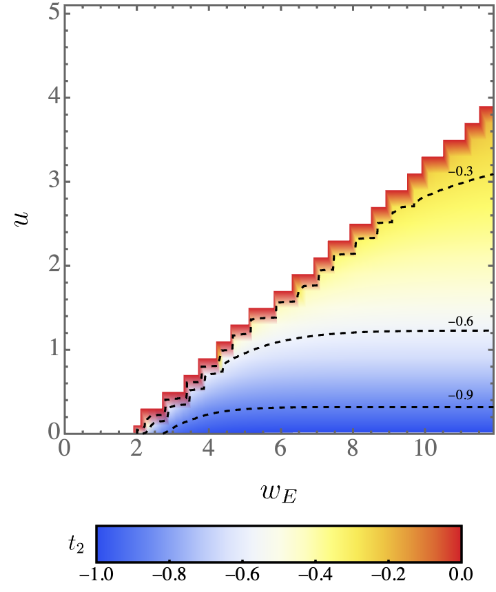
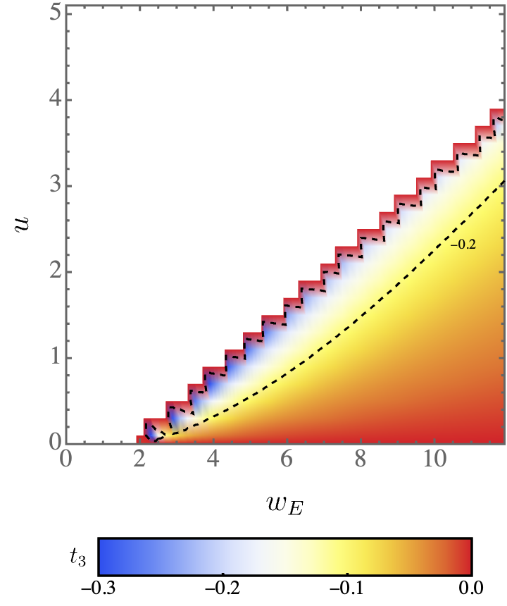
Figure 6: The solutions of the lens eq. (B.5): $t_{1}$ (left), $t_{2}$ (middle), and $t_{3}$ (right), as a function of the impact parameter $u$ and the inverse extent of the lens $w_{\rm E}$.

The numerical result is reported in figure 7 as a function of the ratio between the Einstein ring radius and the size of the lens, $w_{\rm E}\equiv R_{\rm E}/R_{\rm AS}$. The result coincides with the findings obtained through an analytical approximation in ref. [70], so we confirm the validity of such an approximation for the axion star profile.

Figure 7: The threshold impact parameter $u_{1.34}$ as a function of $w_{\rm E}\equiv R_{\rm E}/R_{\rm AS}$ for an axion star.

References

- [1] Planck collaboration, Planck 2018 results. VI. Cosmological parameters, Astron. Astrophys. 641 (2020) A6 [1807.06209].
- [2] Planck collaboration, Planck 2018 results. VIII. Gravitational lensing, Astron. Astrophys. 641 (2020) A8 [1807.06210].
- [3] ACT collaboration, The Atacama Cosmology Telescope: DR6 Gravitational Lensing Map and Cosmological Parameters, Astrophys. J. 962 (2024) 113 [2304.05203].
- [4] DES, SPT collaboration, Joint analysis of Dark Energy Survey Year 3 data and CMB lensing from SPT and Planck. III. Combined cosmological constraints, Phys. Rev. D 107 (2023) 023531 [2206.10824].
- [5] eBOSS collaboration, Completed SDSS-IV extended Baryon Oscillation Spectroscopic Survey: Cosmological implications from two decades of spectroscopic surveys at the Apache Point Observatory, Phys. Rev. D 103 (2021) 083533 [2007.08991].
- [6] P. Natarajan et al., Mapping substructure in the HST Frontier Fields cluster lenses and in cosmological simulations, Mon. Not. Roy. Astron. Soc. 468 (2017) 1962 [1702.04348].
- [7] M. Meneghetti et al., An excess of small-scale gravitational lenses observed in galaxy clusters, Science 369 (2020) 1347 [2009.04471].
- [8] V.C. Rubin, N. Thonnard and W.K. Ford, Jr., Rotational properties of 21 SC galaxies with a large range of luminosities and radii, from NGC 4605 /R = 4kpc/ to UGC 2885 /R = 122 kpc/, Astrophys. J. 238 (1980) 471.
- [9] S. Weinberg, A New Light Boson?, Phys. Rev. Lett. 40 (1978) 223.
- [10] F. Wilczek, Problem of Strong and Invariance in the Presence of Instantons, Phys. Rev. Lett. 40 (1978) 279.
- [11] R.D. Peccei and H.R. Quinn, CP Conservation in the Presence of Instantons, Phys. Rev. Lett. 38 (1977) 1440.
- [12] L. Di Luzio, M. Giannotti, E. Nardi and L. Visinelli, The landscape of QCD axion models, Phys. Rept. 870 (2020) 1 [2003.01100].
- [13] F. Chadha-Day, J. Ellis and D.J.E. Marsh, Axion dark matter: What is it and why now?, Sci. Adv. 8 (2022) abj3618 [2105.01406].
- [14] J. Preskill, M.B. Wise and F. Wilczek, Cosmology of the Invisible Axion, Phys. Lett. B 120 (1983) 127.
- [15] L.F. Abbott and P. Sikivie, A Cosmological Bound on the Invisible Axion, Phys. Lett. B 120 (1983) 133.
- [16] M. Dine and W. Fischler, The Not So Harmless Axion, Phys. Lett. B 120 (1983) 137.
- [17] M. Beltran, J. Garcia-Bellido and J. Lesgourgues, Isocurvature bounds on axions revisited, Phys. Rev. D 75 (2007) 103507 [hep-ph/0606107].
- [18] M.P. Hertzberg, M. Tegmark and F. Wilczek, Axion Cosmology and the Energy Scale of Inflation, Phys. Rev. D 78 (2008) 083507 [0807.1726].
- [19] L. Visinelli and P. Gondolo, Dark Matter Axions Revisited, Phys. Rev. D 80 (2009) 035024 [0903.4377].
- [20] L. Visinelli and P. Gondolo, Axion cold dark matter in non-standard cosmologies, Phys. Rev. D 81 (2010) 063508 [0912.0015].
- [21] T. Hiramatsu, M. Kawasaki, K. Saikawa and T. Sekiguchi, Production of dark matter axions from collapse of string-wall systems, Phys. Rev. D 85 (2012) 105020 [1202.5851].
- [22] V.B.. Klaer and G.D. Moore, The dark-matter axion mass, JCAP 11 (2017) 049 [1708.07521].
- [23] M. Gorghetto, E. Hardy and G. Villadoro, Axions from Strings: the Attractive Solution, JHEP 07 (2018) 151 [1806.04677].
- [24] M. Buschmann, J.W. Foster and B.R. Safdi, Early-Universe Simulations of the Cosmological Axion, Phys. Rev. Lett. 124 (2020) 161103 [1906.00967].
- [25] M. Gorghetto, E. Hardy and G. Villadoro, More axions from strings, SciPost Phys. 10 (2021) 050 [2007.04990].
- [26] M. Buschmann, J.W. Foster, A. Hook, A. Peterson, D.E. Willcox, W. Zhang et al., Dark matter from axion strings with adaptive mesh refinement, Nature Commun. 13 (2022) 1049 [2108.05368].
- [27] S. Hoof, J. Riess and D.J.E. Marsh, Statistical Uncertainties of the QCD Axion Mass Window from Topological Defects, The Open Journal of Astrophysics 5 (2022) 5 [2108.09563].
- [28] K. Saikawa, J. Redondo, A. Vaquero and M. Kaltschmidt, Spectrum of global string networks and the axion dark matter mass, 2401.17253.
- [29] C.J. Hogan and M.J. Rees, AXION MINICLUSTERS, Phys. Lett. B 205 (1988) 228.
- [30] E.W. Kolb and I.I. Tkachev, Nonlinear axion dynamics and formation of cosmological pseudosolitons, Phys. Rev. D49 (1994) 5040 [astro-ph/9311037].
- [31] E.W. Kolb and I.I. Tkachev, Axion miniclusters and Bose stars, Phys. Rev. Lett. 71 (1993) 3051 [hep-ph/9303313].
- [32] E.W. Kolb and I.I. Tkachev, Large amplitude isothermal fluctuations and high density dark matter clumps, Phys. Rev. D 50 (1994) 769 [astro-ph/9403011].
- [33] K.M. Zurek, C.J. Hogan and T.R. Quinn, Astrophysical Effects of Scalar Dark Matter Miniclusters, Phys. Rev. D 75 (2007) 043511 [astro-ph/0607341].
- [34] L. Visinelli and J. Redondo, Axion Miniclusters in Modified Cosmological Histories, Phys. Rev. D 101 (2020) 023008 [1808.01879].
- [35] D. Ellis, D.J.E. Marsh, B. Eggemeier, J. Niemeyer, J. Redondo and K. Dolag, Structure of axion miniclusters, Phys. Rev. D 106 (2022) 103514 [2204.13187].
- [36] A. Vaquero, J. Redondo and J. Stadler, Early seeds of axion miniclusters, JCAP 04 (2019) 012 [1809.09241].
- [37] B. Eggemeier, J. Redondo, K. Dolag, J.C. Niemeyer and A. Vaquero, First Simulations of Axion Minicluster Halos, Phys. Rev. Lett. 125 (2020) 041301 [1911.09417].
- [38] H. Xiao, I. Williams and M. McQuinn, Simulations of axion minihalos, Phys. Rev. D 104 (2021) 023515 [2101.04177].
- [39] B.J. Kavanagh, T.D.P. Edwards, L. Visinelli and C. Weniger, Stellar disruption of axion miniclusters in the Milky Way, Phys. Rev. D 104 (2021) 063038 [2011.05377].
- [40] C.A.J. O’Hare, G. Pierobon and J. Redondo, Axion minicluster streams in the solar neighbourhood, 2311.17367.
- [41] M. Fairbairn, D.J.E. Marsh, J. Quevillon and S. Rozier, Structure formation and microlensing with axion miniclusters, Phys. Rev. D 97 (2018) 083502 [1707.03310].
- [42] D. Croon, D. McKeen and N. Raj, Gravitational microlensing by dark matter in extended structures, Phys. Rev. D 101 (2020) 083013 [2002.08962].
- [43] D. Croon, D. McKeen, N. Raj and Z. Wang, Subaru-HSC through a different lens: Microlensing by extended dark matter structures, Phys. Rev. D 102 (2020) 083021 [2007.12697].
- [44] E.D. Schiappacasse and T.T. Yanagida, Can QCD axion stars explain Subaru HSC microlensing?, Phys. Rev. D 104 (2021) 103020 [2109.13153].
- [45] T.D.P. Edwards, B.J. Kavanagh, L. Visinelli and C. Weniger, Transient Radio Signatures from Neutron Star Encounters with QCD Axion Miniclusters, Phys. Rev. Lett. 127 (2021) 131103 [2011.05378].
- [46] S.J. Witte, S. Baum, M. Lawson, M.C.D. Marsh, A.J. Millar and G. Salinas, Transient radio lines from axion miniclusters and axion stars, Phys. Rev. D 107 (2023) 063013 [2212.08079].
- [47] M.P. Hertzberg, E.D. Schiappacasse and T.T. Yanagida, Axion Star Nucleation in Dark Minihalos around Primordial Black Holes, Phys. Rev. D 102 (2020) 023013 [2001.07476].
- [48] E. Seidel and W.M. Suen, Oscillating soliton stars, Phys. Rev. Lett. 66 (1991) 1659.
- [49] E. Seidel and W.-M. Suen, Formation of solitonic stars through gravitational cooling, Phys. Rev. Lett. 72 (1994) 2516 [gr-qc/9309015].
- [50] D.G. Levkov, A.G. Panin and I.I. Tkachev, Relativistic axions from collapsing Bose stars, Phys. Rev. Lett. 118 (2017) 011301 [1609.03611].
- [51] B. Eggemeier and J.C. Niemeyer, Formation and mass growth of axion stars in axion miniclusters, Phys. Rev. D 100 (2019) 063528 [1906.01348].
- [52] P.H. Chavanis and L. Delfini, Mass-radius relation of Newtonian self-gravitating Bose-Einstein condensates with short-range interactions: II. Numerical results, Phys. Rev. D 84 (2011) 043532 [1103.2054].
- [53] E. Braaten, A. Mohapatra and H. Zhang, Dense Axion Stars, Phys. Rev. Lett. 117 (2016) 121801 [1512.00108].
- [54] L. Visinelli, S. Baum, J. Redondo, K. Freese and F. Wilczek, Dilute and dense axion stars, Phys. Lett. B 777 (2018) 64 [1710.08910].
- [55] E.D. Schiappacasse and M.P. Hertzberg, Analysis of Dark Matter Axion Clumps with Spherical Symmetry, JCAP 01 (2018) 037 [1710.04729].
- [56] M.P. Hertzberg and E.D. Schiappacasse, Dark Matter Axion Clump Resonance of Photons, JCAP 11 (2018) 004 [1805.00430].
- [57] P. Carenza, A. Mirizzi and G. Sigl, Dynamical evolution of axion condensates under stimulated decays into photons, Phys. Rev. D 101 (2020) 103016 [1911.07838].
- [58] M.A. Amin and Z.-G. Mou, Electromagnetic Bursts from Mergers of Oscillons in Axion-like Fields, JCAP 02 (2021) 024 [2009.11337].
- [59] J. Eby, P. Suranyi and L.C.R. Wijewardhana, The Lifetime of Axion Stars, Mod. Phys. Lett. A 31 (2016) 1650090 [1512.01709].
- [60] M. Escudero, C.K. Pooni, M. Fairbairn, D. Blas, X. Du and D.J.E. Marsh, Axion star explosions: A new source for axion indirect detection, Phys. Rev. D 109 (2024) 043018 [2302.10206].
- [61] L. Chung-Jukko, E.A. Lim and D.J.E. Marsh, Multimessenger signals from compact axion star mergers, 2403.03774.
- [62] EROS collaboration, Microlensing towards the small magellanic cloud. eros 2 first year survey, Astron. Astrophys. 332 (1998) 1 [astro-ph/9710194].
- [63] EROS-2 collaboration, Limits on the Macho Content of the Galactic Halo from the EROS-2 Survey of the Magellanic Clouds, Astron. Astrophys. 469 (2007) 387 [astro-ph/0607207].
- [64] MACHO collaboration, The MACHO project: Microlensing results from 5.7 years of LMC observations, Astrophys. J. 542 (2000) 281 [astro-ph/0001272].
- [65] L. Wyrzykowski et al., The OGLE View of Microlensing towards the Magellanic Clouds. IV. OGLE-III SMC Data and Final Conclusions on MACHOs, Mon. Not. Roy. Astron. Soc. 416 (2011) 2949 [1106.2925].
- [66] P. Mroz et al., No massive black holes in the Milky Way halo, 2403.02386.
- [67] I.A. Bond, F. Abe, R.J. Dodd, J.B. Hearnshaw, M. Honda, J. Jugaku et al., Real-time difference imaging analysis of MOA Galactic bulge observations during 2000, Mon. Not. Roy. Astron. Soc. 327 (2001) 868 [astro-ph/0102181].
- [68] D. Croon and S. Sevillano Muñoz, Cosmic microwave background constraints on extended dark matter objects, 2403.13072.
- [69] E.W. Kolb and I.I. Tkachev, Femtolensing and picolensing by axion miniclusters, Astrophys. J. Lett. 460 (1996) L25 [astro-ph/9510043].
- [70] K. Fujikura, M.P. Hertzberg, E.D. Schiappacasse and M. Yamaguchi, Microlensing constraints on axion stars including finite lens and source size effects, Phys. Rev. D 104 (2021) 123012 [2109.04283].
- [71] T. Bringmann, P. Scott and Y. Akrami, Improved constraints on the primordial power spectrum at small scales from ultracompact minihalos, Phys. Rev. D 85 (2012) 125027 [1110.2484].
- [72] V.S. Berezinsky, V.I. Dokuchaev and Y.N. Eroshenko, Formation and internal structure of superdense dark matter clumps and ultracompact minihaloes, JCAP 11 (2013) 059 [1308.6742].
- [73] V.S. Berezinsky, V.I. Dokuchaev and Y.N. Eroshenko, Small-scale clumps of dark matter, Phys. Usp. 57 (2014) 1 [1405.2204].
- [74] J. Adamek, C.T. Byrnes, M. Gosenca and S. Hotchkiss, WIMPs and stellar-mass primordial black holes are incompatible, Phys. Rev. D 100 (2019) 023506 [1901.08528].
- [75] B. Carr, F. Kuhnel and L. Visinelli, Black holes and WIMPs: all or nothing or something else, Mon. Not. Roy. Astron. Soc. 506 (2021) 3648 [2011.01930].
- [76] J.A. Fillmore and P. Goldreich, Self-similiar gravitational collapse in an expanding universe, Astrophys. J. 281 (1984) 1.
- [77] E. Bertschinger, Self - similar secondary infall and accretion in an Einstein-de Sitter universe, Astrophys. J. Suppl. 58 (1985) 39.
- [78] K.J. Mack, J.P. Ostriker and M. Ricotti, Growth of structure seeded by primordial black holes, Astrophys. J. 665 (2007) 1277 [astro-ph/0608642].
- [79] M. Ricotti, J.P. Ostriker and K.J. Mack, Effect of Primordial Black Holes on the Cosmic Microwave Background and Cosmological Parameter Estimates, Astrophys. J. 680 (2008) 829 [0709.0524].
- [80] D.G. Levkov, A.G. Panin and I.I. Tkachev, Gravitational Bose-Einstein condensation in the kinetic regime, Phys. Rev. Lett. 121 (2018) 151301 [1804.05857].
- [81] K. Kirkpatrick, A.E. Mirasola and C. Prescod-Weinstein, Relaxation times for Bose-Einstein condensation in axion miniclusters, Phys. Rev. D 102 (2020) 103012 [2007.07438].
- [82] K. Kirkpatrick, A.E. Mirasola and C. Prescod-Weinstein, Analysis of Bose-Einstein condensation times for self-interacting scalar dark matter, Phys. Rev. D 106 (2022) 043512 [2110.08921].
- [83] J. Chen, X. Du, E.W. Lentz and D.J.E. Marsh, Relaxation times for Bose-Einstein condensation by self-interaction and gravity, Phys. Rev. D 106 (2022) 023009 [2109.11474].
- [84] J. Chen, X. Du, M. Zhou, A. Benson and D.J.E. Marsh, Gravitational Bose-Einstein condensation of vector or hidden photon dark matter, Phys. Rev. D 108 (2023) 083021 [2304.01965].
- [85] A.S. Dmitriev, D.G. Levkov, A.G. Panin and I.I. Tkachev, Self-Similar Growth of Bose Stars, Phys. Rev. Lett. 132 (2024) 091001 [2305.01005].
- [86] M. Jain, W. Wanichwecharungruang and J. Thomas, Kinetic relaxation and nucleation of Bose stars in self-interacting wave dark matter, Phys. Rev. D 109 (2024) 016002 [2310.00058].
- [87] H.-Y. Schive, T. Chiueh and T. Broadhurst, Cosmic Structure as the Quantum Interference of a Coherent Dark Wave, Nature Phys. 10 (2014) 496 [1406.6586].
- [88] H.-Y. Schive, M.-H. Liao, T.-P. Woo, S.-K. Wong, T. Chiueh, T. Broadhurst et al., Understanding the Core-Halo Relation of Quantum Wave Dark Matter from 3D Simulations, Phys. Rev. Lett. 113 (2014) 261302 [1407.7762].
- [89] B. Schwabe, J.C. Niemeyer and J.F. Engels, Simulations of solitonic core mergers in ultralight axion dark matter cosmologies, Phys. Rev. D 94 (2016) 043513 [1606.05151].
- [90] N. Bar, D. Blas, K. Blum and S. Sibiryakov, Galactic rotation curves versus ultralight dark matter: Implications of the soliton-host halo relation, Phys. Rev. D 98 (2018) 083027 [1805.00122].
- [91] E.Y. Davies and P. Mocz, Fuzzy Dark Matter Soliton Cores around Supermassive Black Holes, Mon. Not. Roy. Astron. Soc. 492 (2020) 5721 [1908.04790].
- [92] A. Arvanitaki, M. Baryakhtar and X. Huang, Discovering the QCD Axion with Black Holes and Gravitational Waves, Phys. Rev. D 91 (2015) 084011 [1411.2263].
- [93] C.A.J. O’Hare and A.M. Green, Axion astronomy with microwave cavity experiments, Phys. Rev. D 95 (2017) 063017 [1701.03118].
- [94] D.J. Kaup, Klein-Gordon Geon, Phys. Rev. 172 (1968) 1331.
- [95] R. Ruffini and S. Bonazzola, Systems of selfgravitating particles in general relativity and the concept of an equation of state, Phys. Rev. 187 (1969) 1767.
- [96] J. Enander, A. Pargner and T. Schwetz, Axion minicluster power spectrum and mass function, JCAP 1712 (2017) 038 [1708.04466].
- [97] T. Helfer, D.J.E. Marsh, K. Clough, M. Fairbairn, E.A. Lim and R. Becerril, Black hole formation from axion stars, JCAP 03 (2017) 055 [1609.04724].
- [98] C. Palenzuela, P. Pani, M. Bezares, V. Cardoso, L. Lehner and S. Liebling, Gravitational Wave Signatures of Highly Compact Boson Star Binaries, Phys. Rev. D 96 (2017) 104058 [1710.09432].
- [99] T. Helfer, E.A. Lim, M.A.G. Garcia and M.A. Amin, Gravitational Wave Emission from Collisions of Compact Scalar Solitons, Phys. Rev. D 99 (2019) 044046 [1802.06733].
- [100] J.Y. Widdicombe, T. Helfer, D.J.E. Marsh and E.A. Lim, Formation of Relativistic Axion Stars, JCAP 10 (2018) 005 [1806.09367].
- [101] D. Lai and A.G. Wiseman, Innermost stable circular orbit of inspiraling neutron star binaries: Tidal effects, postNewtonian effects and the neutron star equation of state, Phys. Rev. D 54 (1996) 3958 [gr-qc/9609014].
- [102] G.F. Giudice, M. McCullough and A. Urbano, Hunting for Dark Particles with Gravitational Waves, JCAP 10 (2016) 001 [1605.01209].
- [103] A. Berlin, D. Blas, R. Tito D’Agnolo, S.A.R. Ellis, R. Harnik, Y. Kahn et al., Detecting high-frequency gravitational waves with microwave cavities, Phys. Rev. D 105 (2022) 116011 [2112.11465].
- [104] C. Gatti, L. Visinelli and M. Zantedeschi, Cavity Detection of Gravitational Waves: Where Do We Stand?, 2403.18610.
- [105] M. Maggiore, Gravitational Waves. Vol. 1: Theory and Experiments, Oxford University Press (2007), 10.1093/acprof:oso/9780198570745.001.0001.
- [106] S. Khan, S. Husa, M. Hannam, F. Ohme, M. Pürrer, X. Jiménez Forteza et al., Frequency-domain gravitational waves from nonprecessing black-hole binaries. II. A phenomenological model for the advanced detector era, Phys. Rev. D 93 (2016) 044007 [1508.07253].
- [107] C. Hanna, M.C. Johnson and L. Lehner, Estimating gravitational radiation from super-emitting compact binary systems, Phys. Rev. D 95 (2017) 124042 [1611.03506].
- [108] Y. Kahn, J. Schütte-Engel and T. Trickle, Searching for High Frequency Gravitational Waves with Phonons, 2311.17147.
- [109] A. Ringwald, J. Schütte-Engel and C. Tamarit, Gravitational Waves as a Big Bang Thermometer, JCAP 03 (2021) 054 [2011.04731].
- [110] B. Paczynski, Gravitational Microlensing by the Galactic Halo, Astrophys. J. 304 (1986) 1.
- [111] M.P. Dabrowski and F.E. Schunck, Boson stars as gravitational lenses, Astrophys. J. 535 (2000) 316 [astro-ph/9807039].
- [112] S. Sugiyama, M. Takada and A. Kusenko, Possible evidence of axion stars in HSC and OGLE microlensing events, Phys. Lett. B 840 (2023) 137891 [2108.03063].
- [113] K. Griest, Galactic Microlensing as a Method of Detecting Massive Compact Halo Objects, Astrophys. J. 366 (1991) 412.
- [114] A.H. Guth, M.P. Hertzberg and C. Prescod-Weinstein, Do Dark Matter Axions Form a Condensate with Long-Range Correlation?, Phys. Rev. D92 (2015) 103513 [1412.5930].
- [115] F.S. Guzman and L.A. Urena-Lopez, Evolution of the Schrodinger-Newton system for a selfgravitating scalar field, Phys. Rev. D 69 (2004) 124033 [gr-qc/0404014].
- [116] P.-H. Chavanis, Mass-radius relation of Newtonian self-gravitating Bose-Einstein condensates with short-range interactions: I. Analytical results, Phys. Rev. D84 (2011) 043531 [1103.2050].
- [117] M. Membrado, A.F. Pacheco and J. Sañudo, Hartree solutions for the self-Yukawian boson sphere, Phys. Rev. A 39 (1989) 4207.
- [118] R. Narayan and M. Bartelmann, Lectures on gravitational lensing, in 13th Jerusalem Winter School in Theoretical Physics: Formation of Structure in the Universe, 6, 1996 [astro-ph/9606001].
- [119] R.-G. Cai, T. Chen, S.-J. Wang and X.-Y. Yang, Gravitational microlensing by dressed primordial black holes, JCAP 03 (2023) 043 [2210.02078].
- [120] A. Einstein, Lens-Like Action of a Star by the Deviation of Light in the Gravitational Field, Science 84 (1936) 506.
- [121] H.J. Witt and S. Mao, Can Lensed Stars Be Regarded as Pointlike for Microlensing by MACHOs?, Astrophys. J. 430 (1994) 505.