Robust Snapshot Radio SLAM

Abstract

The intrinsic geometric connections between millimeter-wave (mmWave) signals and the propagation environment can be leveraged for simultaneous localization and mapping (SLAM) in 5G and beyond networks. However, estimated channel parameters that are mismatched to the utilized geometric model can cause the SLAM solution to degrade. In this paper, we propose a robust snapshot radio SLAM algorithm for mixed line-of-sight (LoS) and non-line-of-sight (NLoS) environments that can estimate the unknown user equipment (UE) state, map of the environment as well as the presence of the LoS path. The proposed method can accurately detect outliers and the LoS path, enabling robust estimation in both LoS and NLoS conditions. The proposed method is validated using 60 GHz experimental data, indicating superior performance compared to the state-of-the-art.

I Introduction

The development of evolving 5G and future 6G networks provides not only new opportunities for improving the quality and robustness of communications, but also for facilitating high-accuracy localization and sensing [1, 2]. This is enabled by increased temporal and angular resolution due to the use of higher frequency bands and thus larger bandwidths combined with larger antenna arrays. Extracting timely and accurate location and situational awareness is, in general, a critical asset in various applications such as vehicular systems and industrial mobile work machines [3, 4].

Localization and sensing using downlink/uplink signals between the base station (BS) and user equipment (UE) is often a two-stage process [5], in which the channel parameters, that is, the angle-of-arrival (AoA), angle-of-departure (AoD) and time-of-arrival (ToA) of the resolvable propagation paths are first estimated. Then, in the second stage, the channel parameters are used for localization and sensing. The resolvable non-line-of-sight (NLoS) paths provide information not only about the UE position, but also regarding the incidence point of single-bounce NLoS paths. While these incidence points are unknown, the cardinality of the channel parameters can outweigh the unknowns, enabling bistatic radio simultaneous localization and mapping (SLAM) which aims to estimate the unknown UE state and landmark locations using the channel estimates and the known BS state [6].

The bistatic SLAM problem has gained widespread attention in the 5G/6G research field since it improves localization accuracy [5], enables localizing the UE in the absence of line-of-sight (LoS) [7], and reduces the dependence on infrastructure thus enabling localization even with a single BS [6]. To this end, two mainstream approaches exist in literature: (i) filtering-based solutionsthat recursively estimate the joint state of the UE and map by processing the observations sequentially over time; (ii) snapshot approachesthat solve the SLAM problem for a single UE location without any prior information nor kinematic models. The main benefit of filtering approaches is that higher localization accuracy is expected and state-of-the-art filters [8, 9, 10] can inherently deal with many of the challenges faced in bistatic SLAM including false detections generated by clutter and multi-bounce propagation paths. In contrast, snapshot SLAM is fundamentally important as it serves as a baseline for what can be done with radio signals alone [5, 7, 11, 12] and the solution can be used to initialize and/or as input to filtering approaches. A major limitation of existing snapshot approaches is that they typically overlook outlier measurements that for example originate from multi-bounce propagation paths and that have a mismatch to the utilized geometric model [5, 7, 11, 12]. As a consequence, outliers will cause localization performance degradation.

In this paper, we address the limitations of the state-of-the-art in [5, 7, 11, 12] and develop a novel snapshot SLAM method to estimate the UE state and map of the propagation environment using a single downlink transmission from one BS, that is robust against outlier measurements. The contributions can be summarized as follows:

• We propose a low-complexity processing pipeline for solving the snapshot SLAM problem using measurements that are corrupted by outliers—defined as measurements not originating from LoS or single-bounce NLoS paths;

• We present a method to detect the LoS path and solve the SLAM problem in mixed LoS/NLoS conditions, as opposed to [7, 11] that always assume NLoS;

• Using experimental data with off-the-shelf 60 GHz mmWave MIMO radios, we demonstrate that the developed algorithm can accurately recover the inliers resulting in superior accuracy with respect to the state-of-the-art benchmark algorithms;

• We provide the channel estimates for the experimental data as well as Matlab code that runs the presented method.

II Problem Formulation and Models

Considering the experimental setup in Section IV and to simplify the presentation, we focus on describing the methods in the 2D/azimuth domain but extension to 3D is possible (conceptually similar to, e.g., [7]). The BS state is represented by the position ${\mathbf{p}}_{\textrm{BS}}\in\mathbb{R}^{2}$ and orientation $\alpha_{\textrm{BS}}\in[-\pi,\pi]$. The $i$th landmark is represented by position ${\mathbf{p}}_{i}\in\mathbb{R}^{2}$ which depicts the interaction point of the $i$th single-bounce propagation path. The UE state, ${\mathbf{x}}$, is described using the position ${\mathbf{p}}_{\textrm{UE}}\in\mathbb{R}^{2}$, orientation $\alpha_{\textrm{UE}}$ and clock bias $b_{\textrm{UE}}$.

II-A System Model

Figure 1: Problem geometry for an identifiable system with one LoS and one single-bounce NLoS path. The dashed gray axes define the global coordinate system $(x,\;y)$, angles of the propagation paths are expressed in the local frame of the BS $(x^{\prime},\;y^{\prime})$ and UE $(x^{\prime\prime},\;y^{\prime\prime})$ and the notation is introduced in Section III-A1.

The problem geometry is illustrated in Fig. 1, considering the BS as transmitter and the UE as receiver. We consider beam-based orthogonal frequency-division multiplexing (OFDM) transmission utilizing beam sweeping at both the BS and UE. Assuming coarse timing information for obtaining OFDM symbols within an applicable time window, under which the channel is assumed constant, the received sample of the $l$th OFDM-symbol and $k$th subcarrier with $m$th BS beam and $n$th UE beam can be described as [13]

$$y_{k,l}^{m,n} =\sum_{i=0}^{N}\xi_{i}G^{m}_{\text{BS}}({\phi}_{i})G^{n}_{\text{UE}}({\theta}_{i})e^{-\mathrm{j}2\pi k\Delta\!f\tau_{i}}x_{k,l}^{m,n}+w_{k,l}^{m,n}\!,$$ (1)

where $\Delta f$ is the subcarrier spacing and $w_{k,l}^{m,n}$ denotes noise after applying the UE beam. In addition, $\xi_{i}$, $\tau_{i}$, ${\phi}_{i}$, ${\theta}_{i}$ are the complex path coefficient, ToA, AoD, and AoA for the $i$th propagation path, respectively. Element $i=0$ is reserved for the LoS path (if such is present and detected) and $N$ is the number of NLoS propagation paths. To distinguish between these cases, let the hypothesis $\mathcal{H}=\mathcal{H}_{0}$ represent the LoS condition, while the alternate hypothesis $\mathcal{H}=\mathcal{H}_{1}$ represents the NLoS condition. Furthermore, $G^{m}_{\text{BS}}({\phi}_{i})\!\in\!\mathbb{C}$ and $G^{n}_{\text{UE}}({\theta}_{i})\!\in\!\mathbb{C}$ are angular responses, containing effects of steering vectors and beamformers, for the $m$th BS beam and $n$th UE beam in respective order. Depending on the knowledge of $G^{m}_{\text{BS}}({\phi}_{i})$ and $G^{n}_{\text{UE}}({\theta}_{i})$, various methods for estimating the channel parameters exist [13, 5, 14].

II-B Geometric Measurement Model

Let ${\mathbf{z}}_{i}=[{\tau}_{i},\,{\phi}_{i},\,{\theta}_{i}]^{\top}$ denote the channel parameter estimate of the $i$th propagation path, referred to as ‘measurement’ from now on and let $\mathcal{Z}$ and $\mathcal{I}$ denote a set of measurements and associated indices, respectively. Assuming that the measurement noise is zero-mean Gaussian, which is a common assumption in SLAM [9], the likelihood function is Gaussian

$$p({\mathbf{z}}_{i}\mid{\mathbf{x}},{\mathbf{p}}_{i})=\mathcal{N}({\mathbf{z}}_{i}\mid{\mathbf{h}}({\mathbf{x}},{\mathbf{p}}_{i}),{\mathbf{R}}_{i}),$$ (2)

with mean ${\mathbf{h}}_{i}({\mathbf{x}},{\mathbf{p}}_{i})$ and covariance ${\mathbf{R}}_{i}$. Building on the geometry in Fig. 1, the mean of LoS and single-bounce NLoS paths is given by

$${\mathbf{h}}({\mathbf{x}},{\mathbf{p}}_{i})=\begin{bmatrix}d+b_{\textrm{UE}}\\ \textrm{atan}2(-\delta_{1,y},-\delta_{1,x})-\alpha_{\textrm{BS}}\\ \textrm{atan}2(\delta_{2,y},\delta_{2,x})-\alpha_{\textrm{UE}}\end{bmatrix}$$ (3)

and it represents the geometric relationship between the BS, UE and landmark. For the LoS path $(i=0)$, the parameters are defined as: ${\mathbf{p}}_{i}=\emptyset$, $d=\lVert{\mathbf{p}}_{\textrm{BS}}-{\mathbf{p}}_{\textrm{UE}}\rVert/c$ in which $c$ denotes the speed of light and $[\delta_{1,x},\,\delta_{1,y}]^{\top}=[\delta_{2,x},\,\delta_{2,y}]^{\top}={\mathbf{p}}_{\textrm{BS}}-{\mathbf{p}}_{\textrm{UE}}$. For the $i$th NLoS path, the parameters are defined as: $d=\lVert{\mathbf{p}}_{\textrm{BS}}-{\mathbf{p}}_{i}\rVert/c+\lVert{\mathbf{p}}_{i}-{\mathbf{p}}_{\textrm{UE}}\rVert/c$, $[\delta_{1,x},\,\delta_{1,y}]^{\top}={\mathbf{p}}_{\textrm{BS}}-{\mathbf{p}}_{i}$ and $[\delta_{2,x},\,\delta_{2,y}]^{\top}={\mathbf{p}}_{i}-{\mathbf{p}}_{\textrm{UE}}$.

III Snapshot SLAM

The procedure to solve the SLAM problem depends on $\mathcal{H}$. We first solve the problem considering $\mathcal{H}$ to be known and then the method is generalized to detect the LoS existence.

III-A Snapshot SLAM Without Outliers

To solve the SLAM problem when there are no outliers, we will first assume that the UE orientation is known to provide a conditional estimate, and afterwards estimate the orientation.

III-A1 Conditional Position and Clock Bias Estimate

Let ${\mathbf{x}}_{\alpha_{\textrm{UE}}}=[{\mathbf{p}}_{\textrm{UE}}^{\top},\,b_{\textrm{UE}}]^{\top}$ denote the partial UE state given $\alpha_{\textrm{UE}}$. As illustrated in Fig. 1, the AoD and AoA for a single path can be represented by unit vectors ${\mathbf{u}}_{i}$ and ${\mathbf{v}}_{i}$, given by

$${\mathbf{u}}_{i} ={\mathbf{R}}(\alpha_{\textrm{BS}})\begin{bmatrix}\cos(\phi_{i})&\sin(\phi_{i})\end{bmatrix}^{\top},$$ (4)

$${\mathbf{v}}_{i} ={\mathbf{R}}(\alpha_{\textrm{UE}})\begin{bmatrix}\cos(\theta_{i})&\sin(\theta_{i})\end{bmatrix}^{\top},$$ (5)

in which ${\mathbf{R}}(\alpha)$ is a counterclockwise rotation matrix. Using ${\mathbf{u}}_{i}$ and ${\mathbf{v}}_{i}$, the UE position is given by [7]:

$${\mathbf{p}}_{\textrm{UE}}={\mathbf{p}}_{\textrm{BS}}+d_{i}\gamma_{i}{\mathbf{u}}_{i}-d_{i}(1-\gamma_{i}){\mathbf{v}}_{i}$$ (6)

where $d_{i}=c(\tau_{i}-b_{\textrm{UE}})$ denotes the propagation distance and $\gamma_{i}\in[0,1]$ is unknown and represents the fraction of the propagation distance along ${\mathbf{u}}_{i}$.

The position and clock bias can be estimated utilizing the geometric relationship defined in (6) as follows. First, the expression in (6) can be rearranged as follows

$${\mathbf{H}}_{i}{\mathbf{x}}_{\alpha_{\textrm{UE}}}=\boldsymbol{\mu}_{i}+\gamma_{i}d_{i}\boldsymbol{\nu}_{i}$$ (7)

where ${\mathbf{H}}_{i}=[{\mathbf{I}}_{2\times 2},\,-c{\mathbf{v}}_{i}]$, $\boldsymbol{\mu}_{i}={\mathbf{p}}_{\textrm{BS}}-c\tau_{i}{\mathbf{v}}_{i}$ and $\boldsymbol{\nu}_{i}={\mathbf{u}}_{i}+{\mathbf{v}}_{i}$. Then, we solve for $\gamma_{i}$ and substitute it back to (7) which yields

$${\mathbf{H}}_{i}{\mathbf{x}}_{\alpha_{\textrm{UE}}}=\boldsymbol{\mu}_{i}+\bar{\boldsymbol{\nu}}_{i}^{\top}({\mathbf{H}}_{i}{\mathbf{x}}_{\alpha_{\textrm{UE}}}-\boldsymbol{\mu}_{i})\bar{\boldsymbol{\nu}}_{i},$$ (8)

where $\bar{\boldsymbol{\nu}}_{i}=\bar{\boldsymbol{\nu}}_{i}/\lVert\bar{\boldsymbol{\nu}}_{i}\rVert$. Now, considering all the paths gives the following cost function [11]

$$J({\mathbf{x}}_{\alpha_{\textrm{UE}}}) =\sideset{}{{}_{i\in\mathcal{I}}}{\sum}\eta_{i}J_{i}({\mathbf{x}}_{\alpha_{\textrm{UE}}}),\quad\text{where}$$ (9)

$$J_{i}({\mathbf{x}}_{\alpha_{\textrm{UE}}}) =\lVert{\mathbf{H}}_{i}{\mathbf{x}}_{\alpha_{\textrm{UE}}}-\boldsymbol{\mu}_{i}-\bar{\boldsymbol{\nu}}_{i}^{\top}({\mathbf{H}}_{i}{\mathbf{x}}_{\alpha_{\textrm{UE}}}-\boldsymbol{\mu}_{i})\bar{\boldsymbol{\nu}}_{i}\rVert^{2}$$ (10)

and $\eta_{i}=|\hat{\xi}_{i}|^{2}$ in which $\hat{\xi}_{i}$ denotes the complex path coefficient estimate. Lastly, a closed-form solution can be obtained by setting the gradient of (9) to zero and solving for ${\mathbf{x}}_{\alpha_{\textrm{UE}}}$ as

$$\hat{{\mathbf{x}}}_{\alpha_{\textrm{UE}}}=\left(\sideset{}{{}_{i\in\mathcal{I}}}{\sum}{\mathbf{A}}_{i}\right)^{-1}\sideset{}{{}_{i\in\mathcal{I}}}{\sum}{\mathbf{b}}_{i},$$ (11)

in which ${\mathbf{A}}_{i}=\eta_{i}{\mathbf{H}}_{i}^{\top}\left(\mathbf{I}-\bar{\boldsymbol{\nu}}_{i}\bar{\boldsymbol{\nu}}_{i}^{\top}\right){\mathbf{H}}_{i}$ and ${\mathbf{b}}_{i}=\eta_{i}{\mathbf{H}}_{i}^{\top}\left(\mathbf{I}-\bar{\boldsymbol{\nu}}_{i}\bar{\boldsymbol{\nu}}_{i}^{\top}\right)\boldsymbol{\mu}_{i}$. The SLAM problem is identifiable and all unknowns can be estimated if a sufficient number of NLoS paths exist since each NLoS path provides three measurements, while being parameterized by two unknowns (i.e., ${\mathbf{p}}_{i}$). With known clock bias either the LoS or three NLoS are required [15], whereas one NLoS and the LoS $(N_{\textrm{min}}=2)$ or four NLoS $(N_{\textrm{min}}=4)$ are needed if the BS and UE are not synchronized. Fig. 1 illustrates the problem geometry for an identifiable system with a minimum number of paths and it is important to note that for the LoS path ($i=0$), we have ${\mathbf{v}}_{0}=-{\mathbf{u}}_{0}$, $\bar{\boldsymbol{\nu}}_{0}=\mathbf{0}$ and $\gamma_{0}=1$.

III-A2 Orientation Estimate

The procedure to determine the orientation for both $\mathcal{H}_{0}$ and $\mathcal{H}_{1}$ is described next and the complete state estimate is denoted as $\hat{{\mathbf{x}}}=[\hat{{\mathbf{p}}}_{\textrm{UE}}^{\top},\,\hat{\alpha}_{\textrm{UE}},\,\hat{b}_{\textrm{UE}}]^{\top}$.

1. LoS condition $\mathcal{H}_{0}$ – From Fig. 1, we see immediately that the UE orientation is given by

   $$\hat{\alpha}_{\textrm{UE}}=\textrm{atan}2({y},{x}),$$ (12)

   where $[{x},\;{y}]^{\top}=-{\mathbf{R}}(-\theta_{0}){\mathbf{u}}_{0}$. Hence, the UE positioning problem is solved by first estimating $\hat{\alpha}_{\textrm{UE}}$ using (12) and thereafter, $\hat{{\mathbf{p}}}_{\textrm{UE}}^{\top}$ and $\hat{b}_{\textrm{UE}}$ are estimated using (11).

2. NLoS condition $\mathcal{H}_{1}$ – The problem does not admit a closed-form solution and we must resort to numerical optimization methods as in [7] to obtain the final estimate. Now, the estimate given by (11) can be substituted back into (9) to obtain a cost function over the orientations from which $\hat{{\mathbf{x}}}$ can be found by solving

   $$\hat{\alpha}_{\textrm{UE}}=\underset{{\alpha}_{\textrm{UE}}\in\mathcal{A}}{\textrm{min}\;}J(\hat{{\mathbf{x}}}_{\alpha_{\textrm{UE}}}),$$ (13)

   where $\mathcal{A}$ denotes a grid of possible UE orientations.

III-A3 Landmark Estimate

Given $\hat{{\mathbf{x}}}$, the landmark locations can be estimated by solving a nonlinear optimization problem for every NLoS propagation path $i=1,2,...,N$, independently. The optimization problem is defined as

$$\hat{{\mathbf{p}}}_{i}=\underset{{\mathbf{p}}_{i}}{\textrm{min}\;}({\mathbf{z}}_{i}-{\mathbf{h}}({\mathbf{x}},{\mathbf{p}}_{i}))^{\top}{\mathbf{R}}_{i}^{-1}({\mathbf{z}}_{i}-{\mathbf{h}}({\mathbf{x}},{\mathbf{p}}_{i})),$$ (14)

where ${\mathbf{h}}({\mathbf{x}},{\mathbf{p}}_{i})$ and ${\mathbf{R}}_{i}$ are given in (2). The optimization problem can be solved using the Gauss-Newton algorithm [16] which is initialized using ${\mathbf{p}}_{i}=({\mathbf{p}}_{\textrm{BS},i}+{\mathbf{p}}_{\textrm{UE},i})/2$ where ${\mathbf{p}}_{\textrm{BS},i}$ and ${\mathbf{p}}_{\textrm{UE},i}$ are vectors that span towards ${\mathbf{p}}_{i}$ from the BS, ${\mathbf{p}}_{\textrm{BS},i}={\mathbf{p}}_{\textrm{BS}}+\hat{d}_{i}\hat{\gamma}_{i}\hat{{\mathbf{u}}}_{i}$ and UE, ${\mathbf{p}}_{\textrm{UE},i}=\hat{{\mathbf{p}}}_{\textrm{UE}}+\hat{d}_{i}(1-\hat{\gamma}_{i})\hat{{\mathbf{v}}}_{i}$, respectively, and parameters $\hat{{\mathbf{u}}}_{i}$, $\hat{{\mathbf{v}}}_{i}$, $\hat{d}_{i}$ and $\hat{\gamma}_{i}$ are computed by plugging $\hat{{\mathbf{x}}}$ into (4), (5) and (7).

III-B Robust Snapshot SLAM

The SLAM algorithm described in the previous section is sensitive to measurement outliers. In the worst case, measurements that cannot be expressed using (6) cause the solution to be very inaccurate. In the following, a robust SLAM approach which is inspired by the random sample consensus (RANSAC) algorithm [17] is described. The aim of the robust SLAM algorithm is to find a subset of $\mathcal{Z}$ that does not contain outliers and which is then used to estimate $\hat{{\mathbf{x}}}$. Instead of randomly sampling a subset of $\mathcal{Z}$ as in RANSAC to determine $\hat{{\mathbf{x}}}$, we can perform an exhaustive search over all possible combinations instead, since $\lvert\mathcal{Z}\rvert$ is typically quite low. In the context of RANSAC, minimal solvers that compute solutions from a minimal amount of data, $N_{\textrm{min}}$ in our case, are preferable because it increases the likelihood of using a set that has no outliers. Let, with a slight abuse of notation, $\mathcal{J}_{\textrm{all}}$ denote the set of indices of $\mathcal{Z}$ and $\mathcal{J}\in\mathbb{Z}^{L\times N_{\textrm{min}}}$ the set of all combinations, where $L$ is the total number of combinations

$$L=\frac{(|\mathcal{Z}\rvert-N_{\textrm{LoS}})!}{(|\mathcal{Z}\rvert-N_{\textrm{LoS}}-N_{\textrm{NLoS}})!\,N_{\textrm{NLoS}}!},$$ (15)

in which $N_{\textrm{LoS}}$ and $N_{\textrm{NLoS}}$ denote the minimum number of LoS and NLoS paths required to solve the SLAM problem.

Algorithm 1 Robust snapshot SLAM algorithm

1:Combinations $\mathcal{J}\in\mathbb{Z}^{L\times N_{\textrm{min}}}$, LoS/NLoS condition $\mathcal{H}$, $M$, $\mathcal{Z}$

2:Cost matrix $\mathbf{C}\in\mathbb{R}^{L\times\lvert\mathcal{A}\rvert}$

3:if $\mathcal{H}=\mathcal{H}_{0}$ then $\mathcal{A}=\{0\}$ else $\mathcal{A}=\text{linspace}(-\pi,\pi,M)$

4:for $m=1:\lvert\mathcal{A}\rvert$ do

5:   for $l=1:L$ do

6:      if $\mathcal{H}=\mathcal{H}_{0}$ then $\alpha_{\textrm{UE}}\leftarrow$ (12) else $\alpha_{\textrm{UE}}\leftarrow\{\mathcal{A}\}_{m}$

7:      Set $C_{l,m}=\infty$

8:      Set $\mathcal{I}\leftarrow\{\mathcal{J}\}_{l}$ and compute $\hat{{\mathbf{x}}}_{\alpha_{\textrm{UE}}}$ using (11) based on $\mathcal{I}$

9:      Set $\mathcal{I}_{\textrm{inliers}}=\{i\in\mathcal{J}_{\textrm{all}}\mid J_{i}(\hat{{\mathbf{x}}}_{\alpha_{\textrm{UE}}})\leq T_{\varepsilon}\}$

10:      Set $\mathcal{I}_{\textrm{outliers}}=\mathcal{J}_{\textrm{all}}\setminus\mathcal{I}_{\textrm{inliers}}$

11:      Recompute $\hat{{\mathbf{x}}}_{\alpha_{\textrm{UE}}}$ using (11) based on $\mathcal{I}_{\textrm{inliers}}$

12:      if is_feasible$(\hat{{\mathbf{x}}}_{\alpha_{\textrm{UE}}},\mathcal{I}_{\textrm{inliers}},\mathcal{Z})$ then

$$C_{l,m}=\underbrace{\sum_{i\in\mathcal{I}_{\textrm{inliers}}}\eta_{i}J_{i}(\hat{{\mathbf{x}}}_{\alpha_{\textrm{UE}}})}_{C_{\text{inlier}}}+\underbrace{\sum_{i\in\mathcal{I}_{\textrm{outliers}}}\eta_{i}T_{\varepsilon}}_{C_{\text{outlier}}}$$ (16)

         

13:function is_feasible$({{\mathbf{x}}}_{\alpha_{\textrm{UE}}},\mathcal{I},\mathcal{Z})$

$$j=\textrm{arg\,min}_{i\in\mathcal{I}}\,\{\tau_{i}\}$$

$$\textbf{if }\lvert\mathcal{I}\rvert<N_{\textrm{min}},\textbf{ return false}$$ (17a)

$$\textbf{if }\tau_{j}-{b}_{\textrm{UE}}<0,\textbf{ return false}$$ (17b)

$$\textbf{if }\neg(0\leq\gamma_{i}\leq 1\lor\lVert\boldsymbol{\nu}_{j}\rVert^{2}\leq T_{\boldsymbol{\nu}}),\textbf{ return false}$$ (17c)

$$\textbf{if }\neg(0\leq\gamma_{i}\leq 1),\quad i\in\mathcal{I}\setminus\{j\},\textbf{ return false}$$ (17d)

return true

The robust snapshot SLAM problem is defined as follows. For each set $\mathcal{I}\in\mathcal{J}$ and each value of $\alpha_{\text{UE}}\in\mathcal{A}$ (under $\mathcal{H}_{1}$), the corresponding cost is $\sum_{i\in\mathcal{I}}\eta_{i}J_{i}(\hat{{\mathbf{x}}}_{\alpha_{\textrm{UE}}})$. According to the principles of RANSAC, from the solution $\hat{{\mathbf{x}}}_{\alpha_{\textrm{UE}}}$, the measurements are partitioned into a set of inliers and a set of outliers. A final cost is then computed, denoted by $C(\alpha_{\text{UE}},\mathcal{I})=C_{\text{inlier}}(\alpha_{\text{UE}},\mathcal{I})+C_{\text{outlier}}(\alpha_{\text{UE}},\mathcal{I})$. The penalty $C_{\text{outlier}}(\alpha_{\text{UE}},\mathcal{I})$ is added to ensure that the solution favors estimates obtained with as many inliers as possible. Finally, the optimal solution is found as $\min_{\alpha_{\text{UE}},\mathcal{I}}C(\alpha_{\text{UE}},\mathcal{I})$. The complete method is detailed in Algorithm 1, including the computation of the inlier and outlier cost, as well as the search over minimal index sets $\mathcal{I}$ (indexed by $l$) and UE rotations $\alpha_{\text{UE}}$ (indexed by $m$).

To ensure that the solution is physically meaningful, fundamental feasibility constraints are verified for each solution, given in (17). First, the number of inliers should be sufficient to compute $\hat{{\mathbf{x}}}_{\alpha_{\textrm{UE}}}$ as stated in (17a). Second, the unbiased delay of the shortest path has to be positive as given in (17b). Third, either the shortest path has to follow (6) or unit vectors of the shortest path must be opposite and nearly parallel as given in (17c) in which $T_{\boldsymbol{\nu}}$ is a threshold. Fourth, the constraint in (17d) comes from the definition of ${\mathbf{p}}_{\textrm{UE}}$ in (6).

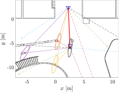
(a) Example solution

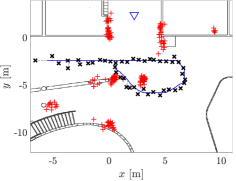
(b) Proposed method

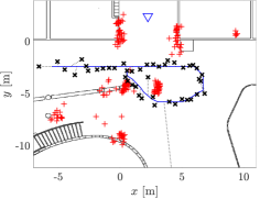
(c) Benchmark method w/o outliers [7]

Figure 2: Example SLAM performance using the proposed and benchmark methods. In (a), the obtained snapshot SLAM solution using the proposed method in one measurement position. In the figure, ${\mathbf{p}}_{\textrm{BS}}$ and ${\mathbf{p}}_{\textrm{UE}}$ illustrated with ( ), $\hat{{\mathbf{p}}}_{\textrm{UE}}$ with ( ), LoS path using ( ), single-bounce NLoS paths with solid lines, propagation paths that are identified as outliers shown using dashed lines (plotted by plugging $\gamma_{i}=0.5$ in to the single-bounce model in (6)) and the dotted ellipses illustrate the one standard deviation uncertainty ellipse of the UE and landmark position estimates. In (b) and (c), $\hat{{\mathbf{p}}}_{\textrm{UE}}$ and $\hat{{\mathbf{p}}}_{i}$’s for all $45$ measurement positions are shown. The legend of the figures is: ${\mathbf{p}}_{\textrm{BS}}$ ( ), ${\mathbf{p}}_{\textrm{UE}}$ ( ), $\hat{{\mathbf{p}}}_{\textrm{UE}}$ ( ) and $\hat{{\mathbf{p}}}_{i}$’s ( ).

III-C Extension to LoS Detection and Mixed LoS/NLoS

Thus far, $\mathcal{H}$ has been assumed known and in the following, the proposed robust snapshot SLAM algorithm is generalized to detect $\mathcal{H}_{0}$ and solve the problem in mixed LoS/NLoS conditions. In this paper, the SLAM problem is solved in mixed LoS/NLoS conditions by first assuming that $\mathcal{H}_{0}$ is true and using a candidate LoS path. Thereafter, a statistical test is performed to validate the obtained solution and if the validation test fails, the SLAM problem is solved again assuming $\mathcal{H}_{1}$. It is to be noted that assuming $\mathcal{H}_{1}$ is always possible, but may lead to performance degradation under $\mathcal{H}_{0}$ as presented in Section IV-B3. First of all, the LoS candidate is the path with smallest delay, $j=\textrm{arg\,min}_{i\in\mathcal{J}_{\textrm{all}}}\,\{\tau_{i}\}$, after which the estimate $\hat{{\mathbf{x}}}$ is obtained using Algorithm 1. Second, we model the LoS signal strength in decibels, $\eta_{j}^{\textrm{dB}}=10\log_{10}(\eta_{j})$, using the log-distance path loss model [18]:

$$\eta_{j}^{\textrm{dB}}\sim\mathcal{N}(f({\mathbf{p}}_{\textrm{UE}}),\sigma^{2}),$$ (18)

where $f({\mathbf{p}}_{\textrm{UE}})=L_{0}+10\,\zeta\log_{10}(\lVert{\mathbf{p}}_{\textrm{BS}}-{\mathbf{p}}_{\textrm{UE}}\rVert)$, $L_{0}$ is the reference path loss at a distance of one meter and $\zeta$ the path loss coefficient. The model parameters ($L_{0},\zeta,\sigma^{2}$) can be learned from training data or derived from existing models (see e.g. [18, Table III]). Third, the utilized statistical test is based on the negative log-likelihood of $\eta_{j}^{\textrm{dB}}$:

$$\frac{1}{2}\left(\log(2\pi\sigma^{2})+\frac{1}{\sigma^{2}}\left(\eta_{j}^{\textrm{dB}}-f(\hat{{\mathbf{p}}}_{\textrm{UE}}))\right)^{2}\right)\underset{\mathcal{H}_{0}}{\overset{\mathcal{H}_{1}}{\gtrless}}T_{\textrm{LoS}}.$$ (19)

If $\mathcal{H}_{0}$ is false, the SLAM problem is re-solved assuming $\mathcal{H}_{1}$.

IV Experimental Results

IV-A Experimental Data and Assumptions

The performance of the proposed and benchmark SLAM algorithms is evaluated using real-world 60 GHz measurement data, obtained indoors at Tampere University campus, with floorplan as illustrated in Fig. 2. Altogether $45$ UE locations were measured—$32$ in LoS and $13$ in NLoS conditions. Beamformed measurements were obtained using $400$ MHz transmission bandwidth utilizing 5G NR-specified downlink positioning reference signals. The details of the experimental setup, hardware and channel estimator are detailed in [13].

The proposed SLAM algorithm utilizes the following parameters in the evaluations. In NLoS conditions, $1^{\circ}$ angle resolution ($\lvert\mathcal{A}\rvert=361$) is used. We utilize the path loss coefficient, $\zeta=1.7$, and standard deviation, $\sigma=1.8\text{ dB}$, of the generic $60$ GHz path loss model [18, Table III] and $L_{0}=13\text{ dB}$ is calibrated from experimental data. The LoS detection threshold in (19) is $T_{\textrm{LoS}}=10.8$ which is computed using the inverse cumulative distribution function of the $\chi^{2}$ distribution with tail probability $0.001$. The inlier detection threshold used in Algorithm 1 is $T_{\varepsilon}=0.1$ and the constraint threshold in (17c) is $T_{\boldsymbol{\nu}}=0.1$. The proposed method is benchmarked with respect to [7] that exploits the closed form solution to estimate the UE position and clock bias introduced in [11]. The benchmark method always assumes $\mathcal{H}_{1}$.

IV-B Results

IV-B1 Qualitative Comparison

The solution in one example measurement position is illustrated in Fig. 2(a) using the proposed robust snapshot SLAM algorithm. In the example, the proposed method can correctly resolve the LoS and single-bounce NLoS paths leading to an accurate SLAM solution in which the UE position estimate is close to the ground truth and the landmark position estimates closely align with the floor plan of the experimental environment. As illustrated in the figure, the propagation paths that are identified as outliers correspond to three double-bounce propagation paths and one triple-bounce propagation path (dashed green line). In all $45$ measurements positions, the proposed method can accurately identify the propagation paths that are inline with model in (6) leading to good SLAM performance as illustrated in Fig. 2(b). Since the benchmark method cannot inherently deal with outliers, they are removed from the data. The SLAM performance for the benchmark method is illustrated in Fig. 2(c) and as shown, the method is clearly not as accurate even without outliers.

IV-B2 Quantitative Comparison

Since the ground truth landmark locations are unknown, which is a common problem in SLAM when using real-world experimental data, the quantitative evaluation focuses on the UE state. The position, heading and clock bias root mean squared errors are tabulated in Table I, and the performance is summarized both with and without outliers. The benchmark method yields poor performance with outliers and the accuracy improves notably without outliers. The proposed method yields equivalent SLAM accuracy in both cases and the results demonstrate that the presented outlier removal method is effective in practice. In the last two rows of Table I, the RMSEs are reported separately in the LoS and NLoS conditions, and as expected, higher accuracy is achieved when the LoS is available.

TABLE I: RMSEs and CPU time of the proposed and benchmark methods.

Method	Pos. [m]	Head. [deg]	Clk. [ns]	Time [ms]
Proposed	$0.36$	$2.05$	$1.45$	$3.02$
Benchmark	$11.12$	$83.79$	$46.52$	$0.96$
Proposed⋆	$0.36$	$2.05$	$1.45$	$0.51$
Benchmark⋆	$1.42$	$4.19$	$4.80$	$0.74$
Proposed†	$0.29$	$1.95$	$1.05$	$0.02$
Proposed‡	$0.49$	$2.27$	$2.13$	$10.40$
⋆data w/o outliers; †LoS condition ($32/45$); ‡NLoS condition ($13/45$).

IV-B3 LoS Detection Accuracy

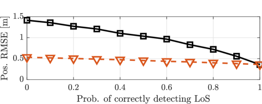
Figure 3: Position RMSE as a function of $P(\mathcal{H}_{0}|\text{LoS})$ and the legend is defined as: RMSE for all $45$ measurement positions ( ) and RMSE computed without ${\mathbf{p}}_{\textrm{UE}}=[3.56,\,-5.70]^{\top}$ ( ).

In the considered experimental setting, the LoS detection routine presented in Section III-C yields perfect detection accuracy, $P(\mathcal{H}_{0}|\text{LoS})=1$ and $P(\mathcal{H}_{1}|\text{NLoS})=1$, but it is to be noted that perfect accuracy is not mandatory. To further investigate SLAM performance with an imperfect LoS detector, we synthetically vary the probability of correctly detecting the LoS, $P(\mathcal{H}_{0}|\text{LoS})\in[0,\,1]$, and perform $1000$ Monte Carlo simulations with each value of $P(\mathcal{H}_{0}|\text{LoS})$. The result is illustrated in Fig. 3. Since the estimate at ${\mathbf{p}}_{\textrm{UE}}=[3.56,\,-5.70]^{\top}$ happens to be very inaccurate if the LoS is misdetected, the RMSE is computed with and without this unfavorable position. Interestingly when $P(\mathcal{H}_{0}|\text{LoS})=0$, the problem is solved assuming NLoS only and the performance is equivalent to the benchmark method without outliers, indicating the proposed method is robust to outliers even without the LoS detector. Furthermore, as $P(\mathcal{H}_{0}|\text{LoS})$ increases, the RMSE decreases which suggests that it is beneficial to solve the problem using the LoS if it exists. The main benefit of using the LoS is that the AoDs and AoAs define the entire geometry up to a scaling since the UE orientation is solved in closed-form and the scaling is determined by the clock bias. In addition, the number of degrees of freedom is lower. Thus, the problem is easier to solve and identifiability of the model is improved leading to increased robustness and enhanced SLAM accuracy when constraints imposed by the LoS are exploited.

IV-B4 Computational Complexity

The computational complexity of the algorithms are given in the last column of Table I, obtained using a Lenovo ThinkPad P1 Gen 2 with a 2.6 GHz Intel i7-9850H CPU and 64 GB of memory. A naive implementation of the proposed and benchmark algorithms scale according to $\mathcal{O}(\lvert\mathcal{A}\rvert\times L)$ and $\mathcal{O}(\lvert\mathcal{A}\rvert)$, respectively. Solving the SLAM problem in LoS conditions using the proposed method is very efficient since $\lvert\mathcal{A}\rvert=1$ and $L=\lvert\mathcal{Z}\rvert-1$. On the other hand, solving the problem is up to three orders of magnitude higher in NLoS conditions since $\lvert\mathcal{A}\rvert=361$ and typically $L$ is much larger. With respect to the benchmark method, the computational complexity of the proposed method is lower/higher in LoS/NLoS condition and real-time operation with both methods can be easily guaranteed using for example a Matlab MEX-implementations as tabulated in Table I.

V Conclusions

The paper presented a robust radio SLAM algorithm for mixed LoS/NLoS environments that can estimate the unknown UE state, incidence point of single-bounce propagation paths, as well as existence of the LoS path, using measurements that are corrupted by outliers. Analysis was carried out using experimental mmWave measurements and the results demonstrated the importance of detecting the outliers and existence of the LoS. The newly proposed radio SLAM algorithm admits numerous possibilities of future research into other mmWave localization and sensing approaches or enhancements via filtering and smoothing.

References

- [1] A. Behravan et al., “Positioning and sensing in 6G: Gaps, challenges, and opportunities,” IEEE Veh. Technol. Mag., vol. 18, no. 1, pp. 40–48, 2023.
- [2] C. De Lima et al., “Convergent communication, sensing and localization in 6G systems: An overview of technologies, opportunities and challenges,” IEEE Access, vol. 9, pp. 26 902–26 925, 2021.
- [3] X. Liu et al., “Robot navigation based on situational awareness,” IEEE Trans. Cogn. Devlop. Syst., vol. 14, no. 3, pp. 869–881, 2022.
- [4] C. Baquero Barneto et al., “Millimeter-wave mobile sensing and environment mapping: Models, algorithms and validation,” IEEE Trans. Veh. Technol., vol. 71, no. 4, pp. 3900–3916, 2022.
- [5] A. Shahmansoori et al., “Position and orientation estimation through millimeter-wave MIMO in 5G systems,” IEEE Trans. Wireless Commun., vol. 17, no. 3, pp. 1822–1835, 2018.
- [6] H. Wymeersch et al., “5G mmWave downlink vehicular positioning,” in IEEE GLOBECOM, 2018, pp. 206–212.
- [7] F. Wen et al., “5G synchronization, positioning, and mapping from diffuse multipath,” IEEE Wireless Commun. Lett., vol. 10, no. 1, pp. 43–47, 2021.
- [8] Y. Ge et al., “A computationally efficient EK-PMBM filter for bistatic mmWave radio SLAM,” IEEE J. Select. Areas Commun., vol. 40, no. 7, pp. 2179–2192, 2022.
- [9] H. Kim et al., “5G mmWave cooperative positioning and mapping using multi-model PHD filter and map fusion,” IEEE Trans. Wireless Commun., vol. 19, no. 6, pp. 3782–3795, Jun. 2020.
- [10] O. Kaltiokallio et al., “Towards real-time radio-SLAM via optimal importance sampling,” in IEEE SPAWC, 2022, pp. 1–5.
- [11] Y. Ge et al., “Experimental validation of single BS 5G mmWave positioning and mapping for intelligent transport,” 2023. [Online]. Available: https://arxiv.org/abs/2303.11995
- [12] M. A. Nazari et al., “mmWave 6D radio localization with a snapshot observation from a single BS,” IEEE Trans. Veh. Technol., vol. 72, no. 7, pp. 8914–8928, 2023.
- [13] E. Rastorgueva-Foi et al., “Millimeter-wave radio SLAM: End-to-end processing methods and experimental validation,” 2023. [Online]. Available: https://arxiv.org/abs/2312.13741
- [14] X. Cheng et al., “Accurate channel estimation for millimeter-wave MIMO systems,” IEEE Trans. Veh. Technol., vol. 68, no. 5, pp. 5159–5163, 2019.
- [15] R. Mendrzik et al., “Harnessing NLOS components for position and orientation estimation in 5G millimeter wave MIMO,” IEEE Trans. Wireless Commun., vol. 18, no. 1, pp. 93–107, 2019.
- [16] S. Boyd et al., Convex Optimization. Cambridge University Press, 2004.
- [17] M. A. Fischler et al., “Random sample consensus: A paradigm for model fitting with applications to image analysis and automated cartography,” Commun. ACM, vol. 24, no. 6, p. 381–395, 1981.
- [18] P. F. M. Smulders, “Statistical characterization of 60-GHz indoor radio channels,” IEEE Trans. Antennas Propag., vol. 57, no. 10, pp. 2820–2829, 2009.