A novel scheme for modelling dissipation or thermalization in open quantum systems
Abstract
In this letter, we introduce a novel method for investigating dissipation or thermalization in an open quantum system. In this method, the quantum system is coupled linearly with a copy of itself or with another system described by a finite number of bosonic operators. The time-dependent coupling functions play a fundamental role in this scheme. To demonstrate the efficacy and significance of this method, we apply it to examine several important and ubiquitous open quantum systems. Firstly, we investigate a quantum oscillator in the presence of a thermal bath at the inverse temperature , obtaining the reduced density matrix, the Husimi distribution function, and the quantum heat distribution function accurately. The results are consistent with existing literature by appropriate choices for the time-dependent coupling function. To illustrate the generalizability of this method to systems interacting with multiple thermal baths, we study the interaction of a quantum oscillator with two thermal baths at different temperatures and obtain compatible results. Subsequently, we analyze a two-level atom with energy or phase dissipation and derive the spontaneous emission and the pure dephasing processes consistently using the new method. Finally, we investigate Markovian and non-Markovian processes in a dissipative two-level atom and observe that these processes depend on the coupling strength , and the non-Markovian property increases with an increase in .
I Introduction
In the fascinating realm of quantum mechanics, understanding how systems interact with their surrounding environment is crucial for various phenomena, ranging from energy transfer processes to the stability of quantum states Feynman2010 . One of the fundamental concepts in this domain is quantum dissipation, which elucidates the dynamics of systems as they lose energy to their surroundings, leading to the gradual decay of their coherence and superposition states Breuer2002 . At its core, quantum dissipation explores the intricate interplay between a quantum system of interest and its surrounding environment, often referred to as a bath Leggett1987 . This interaction introduces a myriad of complex phenomena that challenge traditional classical intuitions. Unlike classical dissipation, where energy loss is typically attributed to macroscopic friction or resistance, quantum dissipation delves into the probabilistic nature of quantum states and their evolution under the influence of environmental perturbations Weiss2012 . A key aspect of quantum dissipation lies in the concept of decoherence, wherein the coherence and superposition of quantum states degrade over time due to interactions with the environment Zurek2003 . This process leads to the emergence of classical-like behavior, effectively erasing the delicate quantum features that distinguish quantum systems from their classical counterparts. Understanding and controlling decoherence is paramount for various applications in quantum information processing, quantum computing, and quantum communication Nielsen2010 . Moreover, the study of quantum dissipation encompasses a rich theoretical framework, drawing from diverse fields such as quantum mechanics, statistical physics, and open quantum systems theory Breuer2002 . Researchers employ various mathematical tools, including master equations, stochastic methods, and quantum field theory, to model and analyze dissipation processes accurately Carmichael1999 . Quantum dissipation finds relevance in a wide array of physical systems, ranging from microscopic quantum circuits and atoms to macroscopic condensed matter systems and cosmological phenomena Leggett1987 . Investigating dissipation mechanisms sheds light on phenomena like relaxation processes, energy transport, and the emergence of irreversible dynamics in quantum systems Weiss2012 . Furthermore, quantum dissipation plays a crucial role in elucidating the behavior of quantum systems far from equilibrium. By probing the dynamics of dissipative quantum systems, researchers gain insights into the emergence of novel phenomena such as quantum phase transitions, nonequilibrium steady states, and quantum criticality Diehl2008 . In conclusion, quantum dissipation stands as a cornerstone in the study of quantum phenomena, offering profound insights into the intricate dynamics of quantum systems interacting with their environment Breuer2002 . By unraveling the mysteries of dissipation, researchers pave the way for harnessing quantum coherence, controlling quantum dynamics, and unlocking the full potential of quantum technologies in the quest for understanding the quantum nature of reality.
II Setting the stage
Consider a quantum system with Hamiltonian described by operators , as the main system. To model loss or thermalization within this system, we linearly couple the main system to either a copy of itself or to a bath system with Hamiltonian , described by a finite set of bosonic operators . The coupling functions are assumed time-dependent. The total Hamiltonian is given by
| (1) |
where the time-dependent coupling functions play a crucial role in the introduced loss or gain scheme. By selecting decreasing coupling functions over time, we demonstrate that the energy flowing from the main system to the bath system cannot completely return to the main system. Moreover, as further elaborated below, the strengths of the coupling functions indicate the Markovian or non-Markovian nature of the process.
III Dissipative harmonic oscillator
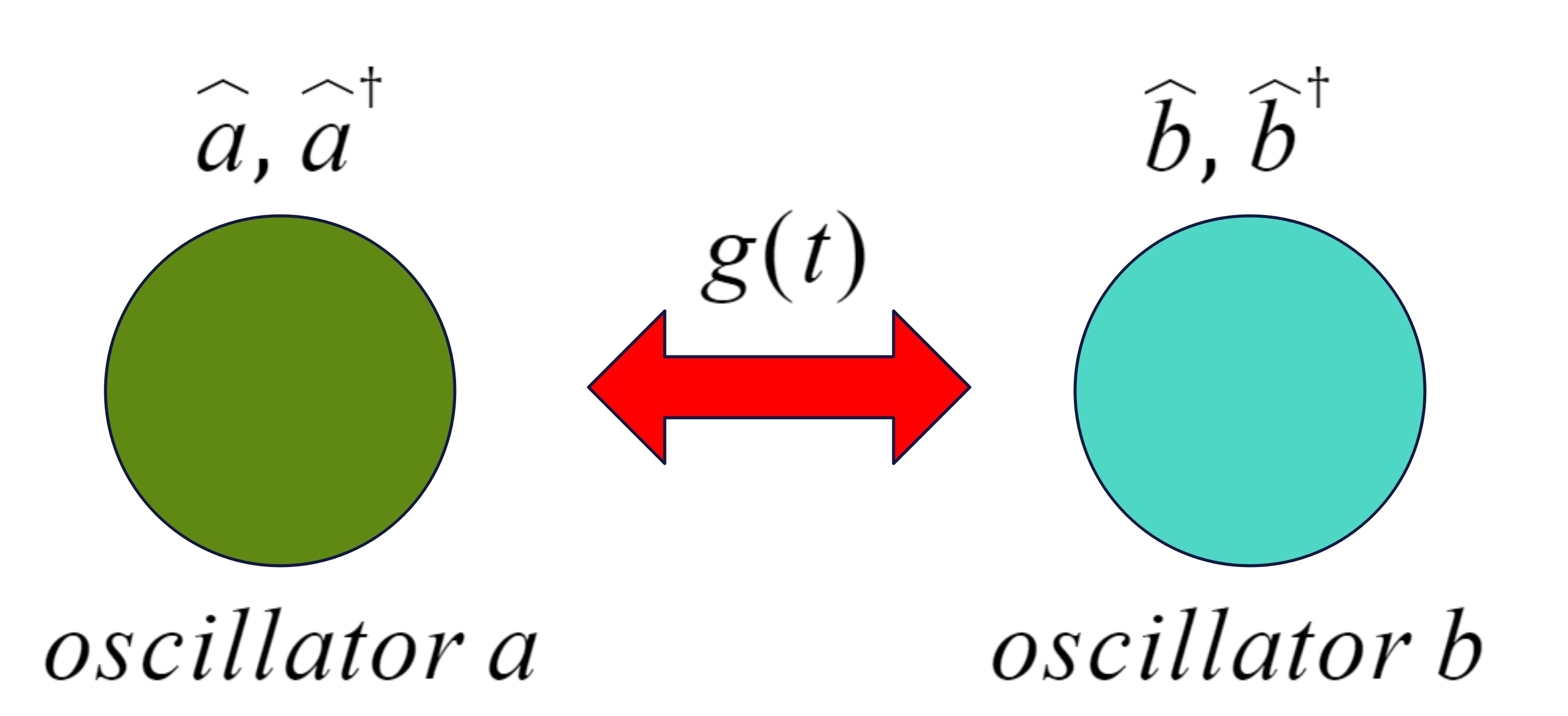
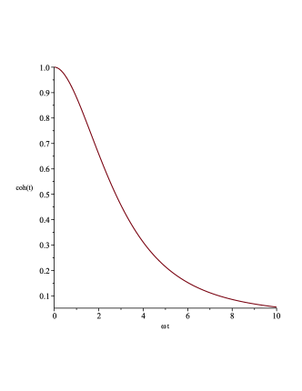
Let’s embark on our journey to demonstrate the effectiveness of the scheme. As our initial example, let’s consider the ubiquitous quantum harmonic oscillator interacting with a heat bath characterized by the inverse temperature Dekker1981 ; Serhan2018 ; Kaur2021 . The bath oscillator mirrors the main oscillator, described by the ladder operators . These two oscillators interact through a time-dependent coupling function , see Fig. (1).
The Hamiltonian is given by
| (2) |
Using the Bogoliubov transformations
| (3) |
the Hamiltonian becomes separable in terms of the new ladder operators
| (4) |
where we have defined , . The time-evolution operator corresponding to Hamiltonian (2) is
| (5) |
where . The time evolution of the total density matrix is described by
| (6) |
where is typically chosen as a separable state . We are interested in the reduced density matrix with components . Let us assume the oscillators are initially prepared in thermal states
| (7) |
where and are the partition functions and inverse temperatures of the oscillators and , respectively. With this choice, we find that the reduced density matrix is a diagonal matrix with the diagonal elements (for details, see SM )
| (8) |
where we defined
| (9) |
In the long-time regime , from (8) and (III) we find
| (10) |
indicating that the -oscillator is thermalized with inverse temperature of the bath, as expected. For a cooling process, let’s assume the bath oscillator (-oscillator) is held at zero temperature. In this case
| (11) |
In the long-time regime , indicating that the -oscillator will finally be found in its ground state, as expected. If we choose
| (12) |
where is a dissipation coefficient, then the energy or equivalently, the mean number , decays exponentially .
If the main oscillator is initially prepared in a coherent state and the bath-oscillator in a thermal state, then
| (13) |
By tracing out the bath oscillator degrees of freedom, we find the Husimi distribution function Schleich2011 corresponding to the reduced density matrix of the main oscillator at time as SM
| (14) |
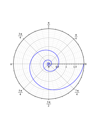
Therefore, the maximum of moves on the path on the complex plane or the phase space, see Fig (2).
III.0.1 Heat distribution of the -oscillator
In the realm of quantum thermodynamics Defner2019 , we revisit the Hamiltonian (2) to explore the heat distribution and its characteristic function for the -oscillator, which is coupled to a heat bath with inverse temperature , while itself maintained at an inverse temperature . The heat distribution function is defined as follows Talkner2007 ; Esposito2009 ; Campisi2011 ; Whitney2014 ; Brander2015 ; Denzler2018 ; Levy2020 ; Funo2018
| (15) |
where ’s are the energy levels of the -oscillator, denotes the probability of the -oscillator being initially at the state , and signifies the transition probability at time for the process . To avoid the complexities associated with the Dirac delta function, it is simpler to use the characteristic function
| (16) |
After straightforward calculations, we find SM
| (17) |
The characteristic function (17) coincides with the result reported in Denzler2018 obtained from Lindblad master equation Lindblad1976 for the choice (12).
IV An oscillator interacting with two baths at different temperatures
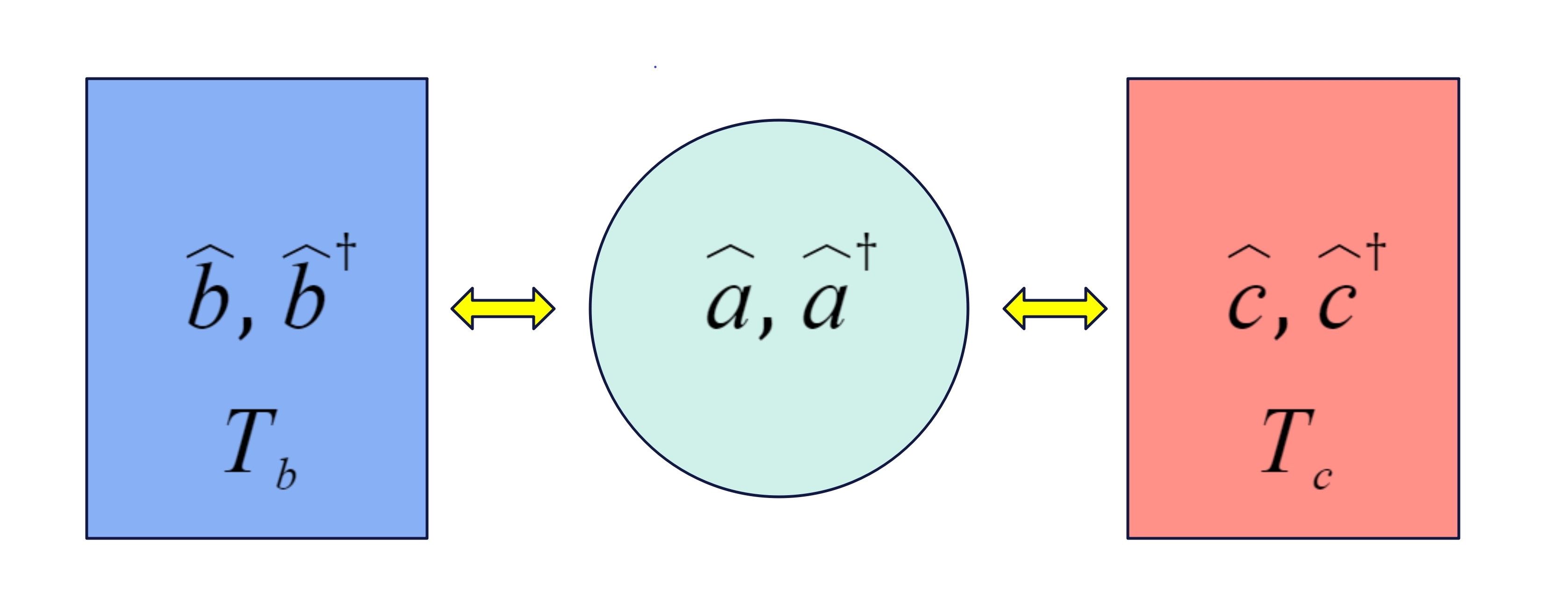
The extension of the scheme to multiple baths is straightforward. For instance, let’s consider an oscillator interacting with two independent baths at inverse temperatures and , as shown in Fig. (3). In this scenario, the total Hamiltonian is given by
| (18) |
Solving the Heisenberg equations of motion yields SM
Suppose the -oscillator is initially in an arbitrary state ; then, the energy of the -oscillator at time is given by
| (20) |
For exponential decay, we set , and in the long-time regime, we find
| (21) |
In the classical regime (), we obtain
| (22) |
as expected.
V Dissipative two-level system
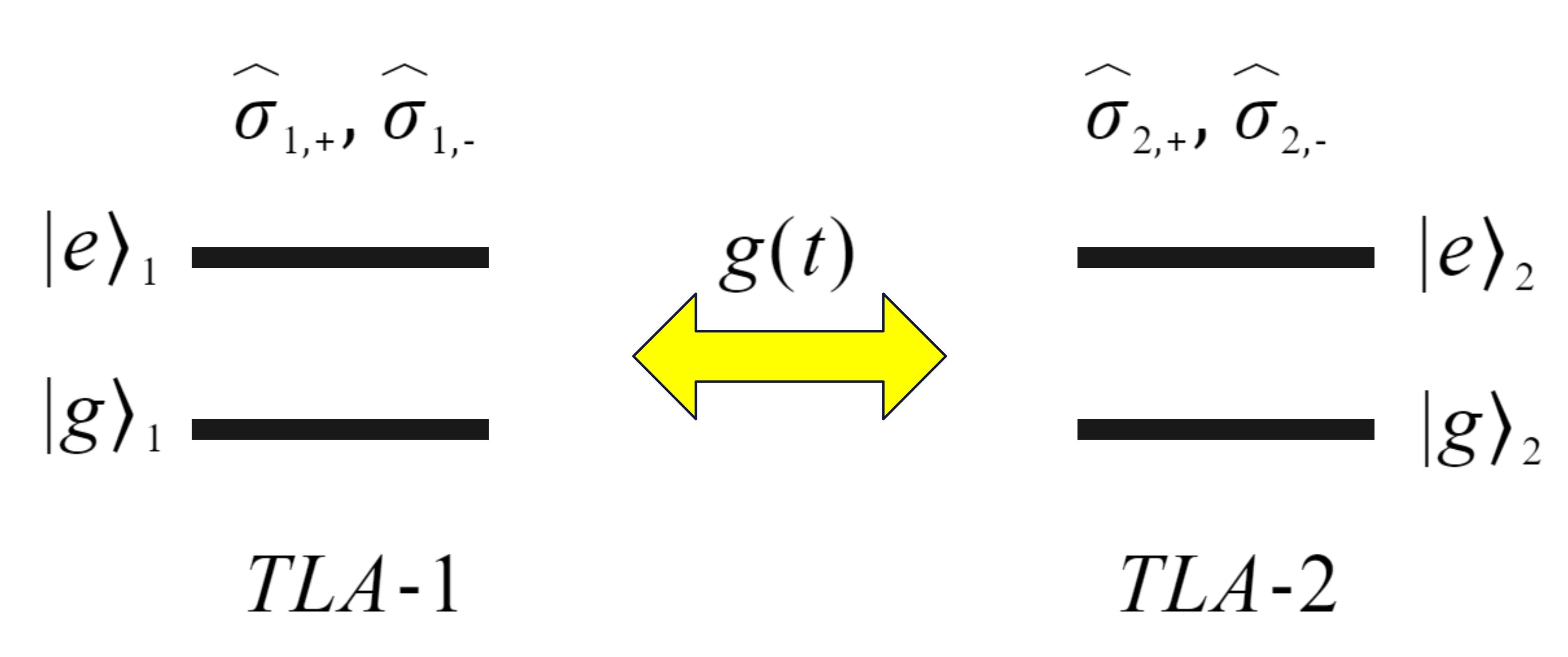
For a dissipative two-level system, we opt to model the bath system as a replica of the main system, as depicted in Fig. (4). Alternatively, we could couple this system to a single bosonic mode, which we will explore in the next section when discussing the pure dephasing model. In both scenarios, the systems interact linearly through a time-dependent coupling function , and the total Hamiltonian is described by
| (23) |
Let us consider the state of the total system at time in the standard basis as
| (24) | |||||
By solving the Schrödinger equation we find the evolution operator in the standard basis as SM
| (25) |
Now, let’s assume that the main system is initially prepared in an arbitrary state
| (26) |
and the bath is initially in the following thermal state
| (27) |
Therefore,
| (32) |
The total density matrix at time is , and by taking the partial trace over the bath degrees of freedom SM , we find
| (34) |
In the long-time regime the main system is thermalized
| (35) |
and when the bath is held in its ground state (), we have
| (36) |
For the particular choice (12), we have and , indicating the spontaneous emission for and , Scully1996 .
VI Pure dephasing model
For pure dephasing model Scully1996 ; Walls2008 ; Manfredi2023 , let us couple the main two-level system to a single bosonic mode as follows
| (37) |
In the interaction picture, we have
| (38) |
Since the Hamiltonian commutes at different times , the evolution operator in the interaction picture can be obtained in closed form as SM
| (39) |
where and is the identity operator. Let the two-level system be initially prepared in an arbitrary state and the bath be hold in a thermal state with inverse temperature
| (40) |
After tracing out the bath degrees of freedom, the reduced density matrix of the main system at an arbitrary time can be obtained as SM
| (41) |
where
| (42) |
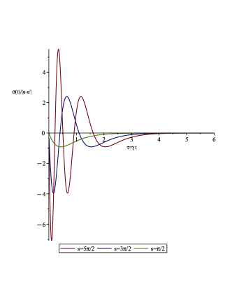
Therefore, the diagonal elements remain unchanged as expected, while the off-diagonal elements decrease by increasing temperature. For the choice , the scaled norm of the off-diagonal element is depicted in terms of the dimensionless variable in Fig. (5), demonstrating a decreasing trend with .
VII Markovian and non-Markovian process
A measure for the distance between two density matrices and is defined by Nielsen2010
| (43) |
where . For a Hermitian matrix (), the trace can be written as a sum over the absolute values of the eigenvalues of , . The rate of change of the distance of evolved density matrices is defined by
| (44) |
A process is said to be non-Markovian Gardiner2004 ; Rivas2014 ; Laine2014 ; Budini2014 ; Breuer2016 ; Vega2017 ; Tamascelli2018 if there exists a pair of initial states and and a certain time such that , Laine2014 . For the dissipative two-level atom let us choose the initial states as
| (45) |
where . The distance between the evolved states is and . In Fig. (6) the function has been depicted for the time-dependent coupling function with different strengths . From Fig. (6), wee see that the non-Markovianity increases by increasing the strength .
VIII Conclusion
In this article, we have introduced a new method for investigating dissipation or thermalization in open quantum systems. This method is based on time-dependent coupling functions, and by appropriately choosing these functions, the effects of dissipation can be modeled on the primary quantum system. To demonstrate the efficiency and simplicity of the method, we examined the quantum dynamics of a harmonic oscillator interacting with a thermal bath for different initial conditions and obtained accurate results for reduced density matrix elements (8), the Husimi distribution function (III), and its phase space representation (Fig. 2), as well as the characteristic heat distribution function for the oscillator (17). These results were consistent with those obtained from other methods such as the Lindblad master equation. To demonstrate the method’s ability to generalize to multiple thermal baths, we investigated the interaction of the oscillator with two thermal baths at different temperatures and obtained compatible results. Furthermore, we examined a two-level atom with energy or phase dissipation and obtained precise results for the reduced density matrices in both cases (34,41, Fig. 5), demonstrating spontaneous emission and pure dephasing processes, respectively. Finally, for the two-level atom, by considering the time-dependent strictly decreasing coupling function , we showed that the non-Markovian property of the process increases with an increase in the intensity of coupling , (Fig. 6). This method can be applied to any desired quantum system in the presence of dissipation or studying thermalization, and the form of the time-dependent coupling functions can be determined based on experimental data. Due to the simplicity of the total Hamiltonian in this scheme, numerical methods will be very effective in cases where the problem is not integrable.
Appendix A Derivation of (8)
Using , we have
| (46) |
by inserting the identity
| (47) |
into equation (A), we obtain
| (48) |
Now, using and the Heisenberg representations
| (49) |
we rewrite (A) as
| (50) |
By making use of the Bogoliubov transformations (3), the Hamiltonian (4), and definitions (), we have
| (51) |
We now employ binomial expansions and assume . Consequently,
For the scenario where both oscillators are initially prepared in thermal states with inverse temperatures and , we obtain
| (53) |
now using
| (54) |
we find
| (55) |
where we used
| (56) |
Hence, the reduced density matrix is diagonal, with its diagonal elements determined by
| (57) |
Appendix B Derivation of (14)
The initial state is given by
| (58) |
The Husimi distribution function corresponding to the reduced density matrix is defined as
| (59) |
where represents the displacement operator, which acts on the vacuum state to produce a coherent state for the -oscillator, denoted by . By utilizing and equation (47), we obtain
| (60) |
To proceed, we substitute equation (A) into equation (B), yielding
| (61) |
where we utilized the following series expansion for Laguerre polynomials
| (62) |
Finally, using the identity
| (63) |
we obtain
| (64) |
Appendix C Derivation of (17)
Appendix D Derivation of (19)
Hamiltonian (18) can be rewritten in matrix form as
| (71) |
The time-dependent matrix exhibits commutativity at distinct times, denoted by , with eigenvalues , , and . The associated renormalized eigenvectors are defined as
| (72) |
The orthogonal matrix generated from these eigenvectors is represented as
| (73) |
We utilize the orthogonal matrix to diagonalize the Hamiltonian and introduce new operators , , and as
| (74) |
The Hamiltonian in terms of the new operators is given by
| (75) |
From the Heisenberg equations of motion for the new operators, we deduce
| (76) |
where . By inverting equation (74), we obtain
| (77) |
Appendix E Derivation of (29)
By substituting the state
| (78) |
into the Schrödinger equation with Hamiltonian (23), we obtain
| (79) |
By employing the new variables
| (80) | |||||
the coupled equations for the coefficients and decouple, and we obtain
| (81) |
In the standard basis, the Schrödinger equation can be expressed in the matrix form as
| (82) |
where the matrix ia unitary evolution matrix (). Suppose the two-level atom is initially prepared in an arbitrary state and the bath is held in a thermal state, then the initial state is expressed as
| (83) |
The total density matrix at an arbitrary time is given by
| (84) |
| (97) | |||
| (102) |
By tracing out the bath degrees of freedom, we find the reduced density matrix as
| (104) |
Appendix F Derivation of (34)
Let the time-dependent operator at the ordered discrete times be denoted by , respectively. Suppose that for any and , the commutator be a -number. Then the generalized form of the Baker-Campbell-Hausdorff formula is expressed as
| (105) |
The evolution operator corresponding to the Hamiltonian (33) in the interaction picture is given by
| (106) |
where represents the time-ordering operator. Since , we can utilize (106) by setting , and rewrite the propagator as
| (107) |
where we defined
| (108) |
Expanding , we obtain
| (109) |
Appendix G Derivation of (36)
References
- (1) R. P. Feynman, A. R. Hibbs, and D. F. Styer, Quantum mechanics and path integrals (Courier Corporation, 2010).
- (2) H. P. Breuer and F. Petruccione, Theory of Open Quantum Systems (Oxford, New York, 2002).
- (3) A. J. Leggett, S. Chakravarty, A. T. Dorsey, M. P. A. Fisher, A. Garg, and W. Zwerger, Dynamics of the dissipative two-state system. Rev. Mod. Phys. 59(1), 1-85 (1987).
- (4) U. Weiss, Quantum dissipative systems, (4th ed.) (World Scientific Publishing Company, 2012).
- (5) W. H. Zurek, Decoherence, einselection, and the quantum origins of the classical, Rev. Mod. Phys. 75(3), 715-775 (2003).
- (6) M. A. Nielsen and I. L. Chuang, Quantum computation and quantum information, (Cambridge University Press, Cambridge, England, 2010).
- (7) H. J. Carmichael, Statistical methods in quantum optics 1: Master equations and Fokker-Planck equations, (Springer Science and Business Media, 1999).
- (8) S. Diehl, A. Micheli, A. Kantian, B. Kraus, H. P. Büchler, and P. Zoller, Quantum states and phases in driven open quantum systems with cold atoms. Nature Physics, 4(11), 878-883 (2008).
- (9) H. Dekker, Classical and quantum mechanics of the damped harmonic oscillator, Phys. Rep. 80(1), 1-10 (1981).
- (10) M. Serhan, M. Abusini, A. Al-Jamel, H. El-Nasser, E. M. Rabei, Quantization of the damped harmonic oscillator, J. Math. Phys. 59(8), (2018).
- (11) J. Kaur, A. Ghosh, and M. Bandyopadhyay, Quantum counterpart of energy equipartition theorem for a dissipative charged magneto-oscillator: Effect of dissipation, memory, and magnetic field, Phys. Rev. E 104, 064112 (2021).
- (12) See Supplementary materials.
- (13) W. P. Schleich, Quantum optics in phase space, (John Wiley and Sons, 2011).
- (14) S. Deffner, S. Campbell, Quantum Thermodynamics: An introduction to the thermodynamics of quantum information, (Morgan and Claypool Publishers, 2019).
- (15) P. Talkner, E. Lutz, and P. Hänggi, Fluctuation theorems: Work is not an observable Phys. Rev. E 75(5), 050102 (2007).
- (16) M. Esposito, U. Harbola, and S. Mukamel, (2009). Nonequilibrium fluctuations, fluctuation theorems, and counting statistics in quantum systems, Rev. Mod. Phys. 81(4), 1665 (2009).
- (17) M. Campisi, J. Pekola, and R. Fazio, Nonequilibrium fluctuations in quantum heat engines: Theory, example, and possible solid state experiments, New J. Phys. 13(3), 033021 (2011).
- (18) R. S. Whitney, Local versus global aspects of heat and work, Phys. Rev. Lett. 112(13), 130601 (2014).
- (19) K. Brandner, K. Saito, and U. Seifert, (2015). Fluctuation and dissipation of work in quantum processes, Phys. Rev. X 5(4), 041019. (2015).
- (20) T. Denzler and E. Lutz, Heat distribution of a quantum harmonic oscillator, Phys. Rev. E 98, 052106 (2018).
- (21) A. Levy and M. Lostaglio, Quasiprobability distribution for heat fluctuations in the quantum regime, PRX Quantum 1, 010309 (2020).
- (22) K. Funo and H. T. Quan, Path integral approach to heat in quantum thermodynamics, Phys. Rev. E 98, 012113 (2018).
- (23) G. Lindblad, On the generators of quantum dynamical semigroups, Commun. Math. Phys. 48, 119 (1976).
- (24) M. Scully and M. S. Zubairy, Quantum Optics (Akademie, Berlin, 1996).
- (25) D. F. Walls and G. J. Milburn, Quantum optics, (2nd ed.), (Springer Science and Business Media, 2008).
- (26) G. Manfredi, A. Rittaud and C. Tronci, Koopman Methods in Classical and Quantum-Classical Mechanics, J. Phys. A: Math. Theor. 56 154002 (2023).
- (27) C. W. Gardiner and P. Zoller, (2004). Quantum noise: A handbook of Markovian and non-Markovian quantum stochastic methods with applications to quantum optics, (3rd ed.), (Springer Science and Business Media, 2004).
- (28) A. Rivas, S. F. Huelga and M. B. Plenio, Quantum non-Markovianity: characterization, quantification and detection, Rep. Prog. Phys. 77(9), 094001 (2014).
- (29) E. M. Laine, J. Piilo and H. P. Breuer, Measure for the degree of non-Markovian behavior of quantum processes in open systems, Phys. Rev. Lett. 108(21), 210402 (2014).
- (30) A. A. Budini, Non-Markovian quantum dynamics of a qubit, Phys. Rev. A 89(5), 052111 (2014).
- (31) H. P. Breuer, E. M. Laine, J. Piilo and B. Vacchini, Colloquium: Non-Markovian dynamics in open quantum systems, Rev. Mod. Phys. 88(2), 021002 (2016).
- (32) I. De Vega and D. Alonso, Dynamics of non-Markovian open quantum systems, Rev. Mod. Phys. 89(1), 015001 (2017).
- (33) D. Tamascelli, A. Smirne, S. F. Huelga and M. B. Plenio, Nonperturbative treatment of non-Markovian dynamics of open quantum systems, Phys. Rev. Lett. 120(3), 030402 (2018).