Tripod: Three Complementary Inductive Biases
for Disentangled Representation Learning

Abstract

Inductive biases are crucial in disentangled representation learning for narrowing down an underspecified solution set. In this work, we consider endowing a neural network autoencoder with three select inductive biases from the literature: data compression into a grid-like latent space via quantization, collective independence amongst latents, and minimal functional influence of any latent on how other latents determine data generation. In principle, these inductive biases are deeply complementary: they most directly specify properties of the latent space, encoder, and decoder, respectively. In practice, however, naively combining existing techniques instantiating these inductive biases fails to yield significant benefits. To address this, we propose adaptations to the three techniques that simplify the learning problem, equip key regularization terms with stabilizing invariances, and quash degenerate incentives. The resulting model, Tripod, achieves state-of-the-art results on a suite of four image disentanglement benchmarks. We also verify that Tripod significantly improves upon its naive incarnation and that all three of its “legs” are necessary for best performance.

1 Introduction

How can we enable machine learning models to process raw perceptual signals into organized concepts similar to how humans do? This intuitively desirable goal has a well-studied formalization known as unsupervised disentangled representation learning: a model is tasked with teasing apart an unlabeled dataset’s underlying sources (a.k.a. factors) of variation and representing them separately from one another, e.g., in independent components of a learned latent space. Beyond aesthetic motivations, achieving disentanglement is a potential stepping stone toward the holy grails of compositional generalization (Bengio, 2013; Wang et al., 2023) and interpretability (Rudin et al., 2022; Zheng & Lapata, 2022). Despite this problem’s importance, there persists a gulf between how well machine learning models and humans disentangle even on carefully curated datasets (Gondal et al., 2019; Nie, 2019).

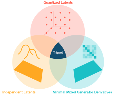
Figure 1: Each of the three inductive biases for disentanglement we consider in this work specifies a different set of preferred models (circles). In principle, using them in conjunction should more precisely specify the desired solution set and better recover models akin to the true data-generating process. Our method, Tripod, makes crucial modifications to these three “legs” to realize this synergy in practice. Code is available at https://github.com/kylehkhsu/tripod.

Inductive biases play a paramount role in enabling disentanglement: they help identify desired solutions amongst the space of all models that explain the data. In this work, we consider three select inductive biases proposed and validated in prior work to have some disentangling effect:

• data compression into a grid-like latent space via quantization (Hsu et al., 2023)

• collective independence amongst latents (Chen et al., 2018; Kim & Mnih, 2018)

• minimal functional influence of any latent on how other latents determine data generation (Peebles et al., 2020)

While each of these desiderata has been shown to improve disentanglement, they achieve unsatisfactory performance in isolation. Since establishing realistic sufficient conditions for identifiability has been a long-standing problem in disentanglement (Locatello et al., 2019; Khemakhem et al., 2020; Horan et al., 2021), it seems prudent to investigate the use of multiple inductive biases in conjunction to more precisely specify the desired solution set.

The key insight this work offers is that the three aforementioned inductive biases, when integrated in a neural network autoencoding framework, are deeply complementary: they most directly specify properties of the latent space, encoder, and decoder, respectively. To elaborate, quantization of the latent space architecturally limits its channel capacity, necessitating efficient communication between the encoder and decoder. Meanwhile, the encoder shapes the joint density of the latents through how it “places” each datapoint, which must be done carefully to achieve collective independence. Finally, the decoder is responsible for minimizing the extent to which latents interact during data generation. Thus, while all three inductive biases ultimately influence the whole model, the mechanism by which each does so is distinct.

Unfortunately, naively combining existing instantiations of these inductive biases results in a model that performs poorly. We conjecture that one key cause of this is an increased difficulty in optimization, a well-known failure mode when juggling multiple objectives in deep learning. Our main technical contribution is a set of adaptations that ameliorate optimization difficulties by simplifying the learning problem, equipping key regularization terms with stabilizing invariances, and quashing degenerate incentives. We now briefly summarize these changes.

Finite scalar latent quantization. We leverage latent quantization to enforce data compression and encourage organization (Hsu et al., 2023), but implement this via finite scalar quantization (Mentzer et al., 2024) instead of dictionary learning (Oord et al., 2017). This fixes the codebook values and obviates two codebook learning terms in the objective, greatly stabilizing training early on and facilitating the optimization of the other inductive biases’ regularization terms.

Kernel-based latent multiinformation. We adapt latent multiinformation regularization, originally proposed for variational autoencoders (Chen et al., 2018; Kim & Mnih, 2018), to be compatible with deterministic encoders without needing an auxiliary discriminator. We achieve this by a novel framing based on kernel density estimation. This allows us to leverage well-known multivariate kernel design heuristics, such as incorporating each dimension’s empirical standard deviation (Silverman, 1998), in order to obtain density estimates that are more useful for multiinformation regularization.

Normalized Hessian penalty. We derive a normalized version of the Hessian (off-diagonal) penalty (Peebles et al., 2020). Unlike the original Hessian penalty, our regularization is invariant to dimensionwise rescaling of the decoder input (latent) and output (activation) spaces. This removes a key barrier to the fruitful application of data-generating mixed derivative regularization to autoencoder architectures, which we demonstrate for the first time; the original Hessian penalty was proposed for generative adversarial networks (GANs), in which the latent space is fixed.

The resulting method, Tripod, establishes a new state-of-the-art on a representative suite of four image disentanglement benchmarks (Burgess & Kim, 2018; Gondal et al., 2019; Nie, 2019) with an InfoMEC $=$ (InfoModularity, InfoCompactness, InfoExplicitness) (Hsu et al., 2023) of $(0.78,0.59,0.90)$ and a DCI $=$ (Disentanglement, Completeness, Informativeness) (Eastwood & Williams, 2018) of $(0.64,0.57,0.93)$ in aggregate. Tripod handidly outperforms methods from previous works that use just one of its component “legs” as well as ablated versions of itself that use two out of three “legs”, validating the premise of using multiple inductive biases in conjunction. We also verify that Tripod disentangles much better than a naive incarnation combining previous instantiations of the three component inductive biases, thereby justifying our technical contributions.

2 Preliminaries

We begin by giving an overview of the specific disentangled representation learning problem we consider in this work. Then, to contextualize our technical contributions and design decisions, we provide detailed descriptions of the previous methods we build upon.

2.1 Disentangled Representation Learning

We consider the following disentangled representation learning problem statement inspired by nonlinear independent components analysis (Hyvärinen & Pajunen, 1999; Zheng et al., 2022; Hsu et al., 2023). Given a dataset of paired samples of sources and data $\{(s,x)\}$ from a true data-generating process

$$p({s})=\prod_{i=1}^{{n_{s}}}p({s}_{i}),\enspace{x}=g({s}),$$ (1)

where ${n_{s}}$ is the number of sources, our aim is to learn an encoder $\hat{{g}}^{-1}:\mathcal{{X}}\to\mathcal{{Z}}$ and decoder $\hat{g}:\mathcal{{Z}}\to\mathcal{{X}}$ solely using the unlabelled data $\mathcal{D}=\{x\}$ such that the latents $z$ recover the sources, thereby disentangling the data. To quantify disentanglement, we will use the InfoMEC (Hsu et al., 2023) and DCI (Eastwood & Williams, 2018) metrics as estimated from samples $\{(s,z=\hat{{g}}^{-1}\circ g(s))\}$ from the joint source-latent distribution $p(s,z)$. Both sets of metrics measure the modularity, compactness, and explicitness of the latents with respect to the sources. InfoM and D measure the extent to which each latent only contains information about one source (i.e., the extent to which the source-latent mapping is one-to-many); InfoC and C the extent to which each source is captured by only one latent (i.e., the extent to which the source-latent mapping is many-to-one); and InfoE and I the extent to which each source can be predicted from the latents with linear or random forest models, respectively. We will also qualitatively inspect models by visualizing the effect of intervening on latents prior to decoding.

2.2 Inductive Biases from Prior Work

Latent quantization. The true sources of variation are a neatly organized, highly compressed representation of the data. Hsu et al. (2023) propose to quantize continuous representations $\hat{{g}}^{-1}(x)$ onto a regular grid to mimic this structure and enforce compression. They accomplish this via a scalar form of vector quantization (VQ; Oord et al. (2017)):

$$z_{j}=\operatorname*{arg\,min}_{e_{jl}\in\mathcal{E}_{j}}\;\lvert\hat{{g}}^{-1}(x)_{j}-e_{jl}\rvert,\enspace j=1,\dots,{n_{z}},$$ (2)

where $\{\mathcal{E}_{j}\}_{j=1}^{n_{z}}$ are the codebook values. These adapt via a “quantization loss” that amounts to dictionary learning, and the continuous values are simultaneously encouraged to collapse to their quantizations via a “commitment loss”:

$$\mathcal{L}_{\text{quantize}}(\{\mathcal{E}_{j}\}) =\lVert\operatorname{StopGrad}(\hat{{g}}^{-1}(x))-z\rVert_{2}^{2},$$ (3)

$$\mathcal{L}_{\text{commit}}(\hat{{g}}^{-1}) =\lVert\hat{{g}}^{-1}(x)-\operatorname{StopGrad}(z)\rVert_{2}^{2}.$$ (4)

Latent multiinformation regularization. Since the true sources are collectively independent (1), biasing the latents towards exhibiting this property should help with recovering something similar to the true generative process. One granular measure of independence is the multiinformation (Studenỳ & Vejnarová, 1998) (a.k.a. total correlation) of the latents,

$$D_{\text{KL}}(q({z})\;\|\;\textstyle\prod_{j=1}^{n_{z}}q({z}_{j})),$$ (5)

which vanishes with perfect collective independence. In a variational autoencoder (VAE; Kingma & Welling (2014)), one can define $q(z)=\frac{1}{|\mathcal{D}|}\sum_{x\in\mathcal{D}}q(z|x)$ to be an “aggregate posterior”. Since naive Monte Carlo estimation of the multiinformation would require the entire dataset, Chen et al. (2018) design a minibatch-weighted estimator for the expected log density:

$$\mathbb{E}_{z\sim q(z)}[\log q(z)]\approx\frac{1}{{n_{b}}}\sum_{i_{1}=1}^{{n_{b}}}\log\frac{1}{{n_{b}}|\mathcal{D}|}\sum_{i_{2}=1}^{{n_{b}}}q\left(z^{(i_{2})}|x^{(i_{1})}\right),$$ (6)

where ${n_{b}}$ is the batch size and $|\mathcal{D}|$ is the dataset size. They handle the marginals $q(z_{j})$ analogously, and add the estimated multiinformation as a regularization term to the VAE evidence lower bound objective.

Data-generating mixed derivative regularization. Peebles et al. (2020) propose that, in a data-generating process that transforms latents into data, each latent should minimally affect how any other latent functionally influences the data. To accomplish this, they regularize the mixed derivatives of the generator in a generative adversarial network (Goodfellow et al., 2014) (GAN):

$$\min_{\hat{g}^{[k]}}\sum_{j_{1}\neq j_{2}}\left(H^{[k]}_{j_{1}j_{2}}\right)^{2}$$ (7)

where $\hat{g}^{[k]}$ denotes some generator activation or output dimension and $H^{[k]}$ is the corresponding Hessian with respect to the latents. Naively implementing this via automatic differentiation is too computationally expensive, as it would involve taking third-order derivatives for first-order optimization schemes. Instead, Peebles et al. (2020) apply a Hutchinson-style unbiased estimator for the sum of the squared off-diagonal elements of a matrix (Hutchinson, 1989):

$$\operatorname*{Var}_{v\sim\operatorname{Rademacher}(1)}[v^{\top}H^{[k]}v]=2\sum_{j_{1}\neq j_{2}}\left(H^{[k]}_{j_{1}j_{2}}\right)^{2},$$ (8)

as well as a central finite difference approximation for the second-order directional derivative:

$$v^{\top}H^{[k]}v\approx\frac{\hat{g}^{[k]}(z+\epsilon v)-2\hat{g}^{[k]}(z)+\hat{g}^{[k]}(z-\epsilon v)}{\epsilon^{2}}.$$ (9)

3 The Three Legs of Tripod

In this section, we describe the design decisions we make in order to successfully meld latent quantization, latent multiinformation regularization, and data-generating mixed derivative regularization together in a single model. Our overarching design principle is as follows: we want each inductive bias to do its job with the lightest touch possible in order to avoid “interference” and ease optimization.

3.1 Finite Scalar Latent Quantization (FSLQ)

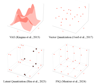
Figure 2: The evolution of discrete latent space structure in autoencoders. We use finite scalar quantization (bottom right) instead of latent quantization (bottom left) so that the codebook values need not be learned.

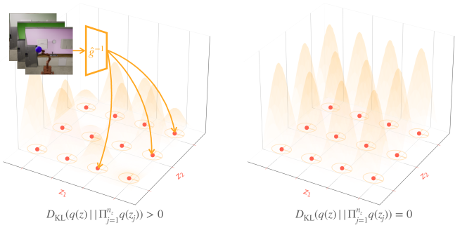
Figure 3: Kernel density estimation facilitates regularizing deterministic quantized latents from having nonzero multiinformation (left) towards collective independence (right). The multiinformation estimation smoothly depends on the latents through distances between samples (11, 13). The smoothing matrix $S$ (12) is visualized with a level set (ellipse) of each latent sample’s kernel density, and incorporates each dimension’s scale (ellipse major and minor axes). The visualized joint densities illustrate the result of accumulating latent sample kernel densities at each grid point.

The scalar form of VQ that Hsu et al. (2023) use to instantiate latent quantization (LQ) requires a quantization loss (3) for learning the discrete codebook values and a commitment loss (4) to regularize the continuous values. We are looking to include other regularizers on the latents that more directly enable disentanglement, and these would play a bigger role in the objective if the VQ losses could be removed. The recently proposed finite scalar quantization  (FSQ; Mentzer et al. (2024)) scheme identifies a recipe for doing this using fixed codebook values and judiciously chosen mappings pre- and post-quantization. We graphically depict VQ, LQ, and FSQ in Figure 2.

We implement a variant of FSQ that has the continuous and quantized latent spaces share the same ambient “bounding box”. The continuous latent space is specified as $[-1,1]^{n_{z}}$ by applying the hyperbolic tangent function to the output of the encoder network. Latent vectors are then linearly rescaled to $[0,{n_{q}}-1]^{n_{z}}$, rounded elementwise to the nearest integer, and unscaled. Concretely, the quantization operation is

$$z=\frac{2}{{n_{q}}-1}\operatorname{round}\left(\frac{{n_{q}}-1}{2}\left(\tanh\left(\hat{{g}}^{-1}\left(x\right)\right)+1\right)\right)-1,$$ (10)

where ${n_{q}}$ is the number of discrete values in each dimension. The straight-through gradient trick (Bengio et al., 2013) is used to copy gradients across the nondifferentiable rounding operation.

FSQ directly obviates the quantization loss (3) as the latent codebook is fixed to $\{-1,-1+\frac{2}{{n_{q}}-1},\dots,1\}^{n_{z}}$. Mentzer et al. (2024) empirically show that the commitment loss (4) also becomes unnecessary. These simplifications greatly stabilize the early periods of training and “make room” for the other two inductive biases, which we discuss next.

3.2 Kernel-Based Latent Multiinformation (KLM)

At face value, the idea of regularizing latent multiinformation (5) à la Chen et al. (2018) appears to be incompatible with deterministic latents: since each “posterior” is a Dirac delta function, we have $q(z)=\frac{1}{|\mathcal{D}|}\sum_{x\in\mathcal{D}}\delta(z-\hat{{g}}^{-1}(x))$, which has a support of measure zero. We instead adopt a perspective of doing kernel density estimation (KDE) using a finite data sample: we specify a kernel-based smoothing of the Dirac deltas for the express purpose of obtaining smoothly parameterized density estimates that are amenable to gradient-based optimization. See Figure 3 for an illustration of our method. We make the standard choice of Gaussian kernel functions; concretely, we estimate the joint density as

$$q(z)=\frac{1}{n_{b}}\sum_{i=1}^{n_{b}}\frac{1}{(2\pi)^{\frac{{n_{z}}}{2}}|S|^{\frac{1}{2}}}\exp\left(-\frac{1}{2}f(z-z^{(i)};S)\right),$$ (11)

where $f(z^{\prime};S)=z^{\prime\top}S^{-1}z^{\prime}$ and $S$ is a smoothing matrix. In KDE, it is a common heuristic to incorporate the empirical standard deviation of each dimension $\sigma_{j}$ into the kernel smoothing parameters (Silverman, 1998). This specifies an invariance to the dimensionwise scaling, facilitating, e.g., latent shrinkage without adversely affecting multiinformation estimation. Specifically, to estimate the joint density $q(z)$, we use Silverman’s rule of thumb for each nonzero element of the diagonal smoothing matrix:

$$S_{jj}=\left(\frac{4}{({n_{z}}+2){n_{b}}}\right)^{\frac{2}{{n_{z}}+4}}\sigma_{j}^{2}.$$ (12)

For estimating the marginal densities, we again use $\sigma_{j}$ as the smoothing parameter:

$$q(z_{j})=\frac{1}{n_{b}}\sum_{i=1}^{n_{b}}\frac{1}{\sqrt{2\pi}\sigma_{j}}\exp\left(-\frac{1}{2}\left(\frac{z_{j}-z_{j}^{(i)}}{\sigma_{j}}\right)^{2}\right).$$ (13)

We now have satisfactory approximations for the densities involved in computing latent multiinformation (5). Our batch log joint density estimator,

$$\mathbb{E}_{z\sim q(z)}[\log q(z)]\approx\frac{1}{{n_{b}}}\sum_{i_{1}=1}^{{n_{b}}}\log\frac{1}{{n_{b}}}\sum_{i_{2}=1}^{{n_{b}}}K_{S}\left(z^{(i_{2})}-z^{(i_{1})}\right)$$ (14)

ultimately takes a highly similar form to the minibatch-weighted estimator (6) of Chen et al. (2018), except the pairwise interaction between samples arises from kernel-based smoothing rather than uncertainty in posterior inference. We also avoid the inclusion of the dataset size due to not using an importance sampling derivation. Cosmetic differences aside, the two methods are deeply related: one can view the design of the variational posterior $q$ as analogous to the design of the kernel $K_{S}$. We remark that KLM is designed for deterministic latents taking on values in $\mathbb{R}^{{n_{z}}}$. This includes our quantized latents as a specific case thanks to the design of the quantized latent space in Section 3.1.

As an alternative to kernel-based smoothing, we can consider treating the quantized latents as categorical variables, but we find that the required machinery, e.g., Gumbel-Softmax reparameterization (Jang et al., 2017; Maddison et al., 2017), is significantly more unwieldy to use in practice compared to kernel density estimation.

3.3 Normalized Hessian Penalty (NHP)

Algorithm 1 Pseudocode for the Tripod objective. We use ${n_{b}}=64,{n_{p}}=2,\epsilon=0.1$ throughout and tune $(\lambda_{\text{KLM}},\lambda_{\text{NHP}})$.

1:  given: batch size ${n_{b}}$, data $\{x^{(i)}\}_{i=1}^{{n_{b}}}$, encoder $\hat{{g}}^{-1}$, decoder $\hat{g}$, number of perturbations ${n_{p}}$, perturbation parameter $\epsilon$ given: regularization weights $(\lambda_{\text{KLM}},\lambda_{\text{NHP}})$

2:  for $i\in[{n_{b}}]$ do

3:     $c^{(i)}\leftarrow\hat{{g}}^{-1}(x^{(i)})$ {encode data into continuous latent vectors}

4:      $z^{(i)}\leftarrow\operatorname{Quantize}\left(c^{(i)}\right)$ {apply finite scalar quantization (10)}

5:  end for

6:   $\mathcal{L}_{\text{reconstruction}}\leftarrow\frac{1}{{n_{b}}}\sum_{i=1}^{n_{b}}\operatorname{BinaryCrossEntropy}\left(\hat{g}(z^{(i)}),x^{(i)}\right)$

7:  $\sigma_{j}\leftarrow\operatorname{std}\left(c^{(1)}_{j},\dots,c^{({n_{b}})}_{j}\right)\ \forall j\in[{n_{z}}]$ {calculate the empirical standard deviation of each latent dimension}

8:   $S\leftarrow\operatorname{Silverman^{\prime}s}\left(\sigma_{1},\dots,\sigma_{{n_{z}}},{n_{b}},{n_{z}}\right)$ {form joint density smoothing matrix (12)}

9:  for $i\in[{n_{b}}]$ do

10:      $q^{(i)}\leftarrow\operatorname{KDE}\left(z^{(i)};z^{(1)},\dots,z^{({n_{b}})},S\right)$ {joint KDE (11)}

11:      $q_{j}^{(i)}\leftarrow\operatorname{KDE}\left(z_{j}^{(i)};z^{(1)}_{j},\dots,z^{({n_{b}})}_{j},\sigma_{j}\right)\forall j\in[{n_{z}}]$ {marginal KDEs (13)}

12:  end for

13:   $\mathcal{L}_{\text{latent multiinformation}}\leftarrow\frac{1}{{n_{b}}}\sum_{i=1}^{n_{b}}\left(\log q^{(i)}-\sum_{j=1}^{n_{z}}\log q_{j}^{(i)}\right)$

14:  for $i\in[{n_{b}}],k\in\{\text{regularized decoder activation dimensions}\}$ do

15:     for $l\in{n_{p}}$ do

16:         $v^{(i)}_{jkl}\leftarrow\sigma_{j}\operatorname{SampleRademacher}(1)\ \forall j\in[{n_{z}}]$ {scale-adjusted sampling (Proposition 3.2)}

17:         $w^{(i)}_{jkl}\leftarrow\sigma_{j}\operatorname{SampleNormal}(0,1)\ \forall j\in[{n_{z}}]$

18:         $\text{numer}f^{(i)}_{kl}\leftarrow\operatorname{FiniteDifferences}\left(\hat{g}^{[k]},z^{(i)},\epsilon,v^{(i)}_{kl}\right)$ {estimate curvature (9)}

19:         $\text{denom}f^{(i)}_{kl}\leftarrow\operatorname{FiniteDifferences}\left(\hat{g}^{[k]},z^{(i)},\epsilon,w^{(i)}_{kl}\right)$

20:     end for

21:      $\text{numer}f^{(i)}_{k}\leftarrow\operatorname{var}\left(\text{numer}f^{(i)}_{k1},\dots,\text{numer}f^{(i)}_{k{n_{p}}}\right)$ {calculate empirical variance across perturbations (17)}

22:      $\text{denom}f^{(i)}_{k}\leftarrow\operatorname{var}\left(\text{denom}f^{(i)}_{k1},\dots,\text{denom}f^{(i)}_{k{n_{p}}}\right)$

23:  end for

24:   $\mathcal{L}_{\text{normalized Hessian penalty}}\leftarrow\frac{1}{{n_{b}}}\sum_{i=1}^{n_{b}}\frac{\sum_{k}\text{numer}f^{(i)}_{k}}{\sum_{k}\text{denom}f^{(i)}_{k}}$

25:  return: $\mathcal{L}_{\text{}}\leftarrow$ $\mathcal{L}_{\text{reconstruction}}$ $+$ $\lambda_{\text{KLM}}\mathcal{L}_{\text{latent multiinformation}}$ $+$ $\lambda_{\text{NHP}}\mathcal{L}_{\text{normalized Hessian penalty}}$

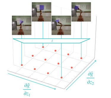
Figure 4: The Hessian penalty is supposed to specify a preference for decoders, such as the one depicted, in which change along one latent (object shape) minimally affects how another latent (horizontal end-effector position) influences data generation. We modify the Hessian penalty to quash degenerate solutions that compromise this intended outcome in autoencoders.

The original Hessian penalty (8) amounts to reducing the magnitudes of mixed derivatives in a learned data-generating function (Figure 4). Unfortunately, this can be trivially achieved by scaling down activations or scaling up latents, circumventing the intended effect of making the Hessians more diagonal. Indeed, the former degeneracy is likely why Peebles et al. (2020) find it important to use normalization layers immediately preceding activations used for regularization: in experiments with the original Hessian penalty, we find that it causes the norms of regularized activations to decrease. More importantly, the latter degeneracy may be why the Hessian penalty has not seen fruitful application in autoencoders: the decoder input space is variable and hence susceptible, whereas the input space of a GAN’s generator is fixed.

We would like to rule out trivial scaling-based solutions to data-generating mixed derivative regularization by making the regularization term invariant to the scale of any individual input (latent) or output (activation). We endow the Hessian penalty with these properties by incorporating the standard deviations of the latents in each second derivative and normalizing by an aggregation of all second derivatives. This is formalized in Proposition 3.1.

Proposition 3.1.

The Hessian penalty

$$\sum_{j_{1}\neq j_{2}}\left(H^{[k]}_{j_{1}j_{2}}\right)^{2}$$ (15)

can be reduced by scaling down $\hat{g}{}_{k}$ or scaling up any $z_{j},j\in[{n_{z}}]$, and vice versa. In contrast, the normalized Hessian penalty

$$\frac{\sum_{j_{1}\neq j_{2}}\left(H^{[k]}_{j_{1}j_{2}}\sigma_{j_{1}}\sigma_{j_{2}}\right)^{2}}{\sum_{j_{1},j_{2}}\left(H^{[k]}_{j_{1}j_{2}}\sigma_{j_{1}}\sigma_{j_{2}}\right)^{2}}$$ (16)

is invariant to the scaling of $\hat{g}^{[k]}$ and $z_{j}\ \forall j\in[{n_{z}}]$.

Proof.

See Section A.1. ∎

However, incorporating the latent standard deviations into each term is nontrivial since the Hutchinson-style estimation (8) never explicitly forms any of the terms in the sum. We also need a way of estimating the denominator of (16), which includes the Hessian’s squared diagonal entries. Fortunately, each can be achieved with a judicious change to the sampling distribution, as we show in Proposition 3.2.

Proposition 3.2.

Let $v$ and $w$ be random vectors where $v_{j}\sim\operatorname{Rademacher}(\sigma_{j})$ and $w_{j}\sim\mathcal{N}(0,\sigma_{j}^{2})$. Then the normalized Hessian penalty can be computed as

$$\frac{\sum_{j_{1}\neq j_{2}}\left(H^{[k]}_{j_{1}j_{2}}\sigma_{j_{1}}\sigma_{j_{2}}\right)^{2}}{\sum_{j_{1},j_{2}}\left(H^{[k]}_{j_{1}j_{2}}\sigma_{j_{1}}\sigma_{j_{2}}\right)^{2}}=\frac{\operatorname*{Var}\left[v^{T}H^{[k]}v\right]}{\operatorname*{Var}\left[w^{T}H^{[k]}w\right]}.$$ (17)

Proof.

See Section A.2. ∎

Using a central finite difference approximation (9) for the second-order directional derivatives (17), we are now able to estimate the normalized Hessian penalty (16) just with forward passes through the decoder $\hat{g}(z)$. Compared to the original Hessian penalty, this incurs twice as many forward passes per optimization step.

3.4 Implementation Details

In Algorithm 1, we provide pseudocode for computing the Tripod objective. There are a few implementation details worth noting. We compute the latents’ empirical standard deviation based on the continuous values to avoid obtaining a value of zero for a batch. Substituting the statistics of one for the other is facilitated by tying together the continuous and quantized latent spaces as outlined in Section 3.1. However, for the kernel density estimates and finite differences, we use the quantized latents. Also, due to the low number of perturbations (2) used for the curvature approximations, we find it more stable to separately aggregate the numerators and denominators of the normalized Hessian penalties for each decoder activation dimension before division. For the degree of quantization ${n_{q}}$, we use a fixed value of $12$, except when we ablate this hyperparameter specifically. Finally, while we explicitly write out nested loops in Algorithm 1 to maximize clarity, in code these are vectorized for the sake of efficiency.

Table 1: Tripod achieves state-of-the-art disentanglement as quantified by InfoMEC and DCI (the former is re-ordered to align with the latter). See Section 4.2 for detailed commentary.

model	aggregated			Shapes3D			MPI3D			Falcor3D			Isaac3D
	$\text{InfoMEC}:=(\text{InfoM}\ \text{InfoC}\ \text{InfoE})$
$\beta$-TCVAE	$(0.62$	$\mathbf{0.57}$	$0.77)$	$(0.68$	$0.55$	$\mathbf{0.98})$	$(0.45$	$0.42$	$0.61)$	$(0.71$	$\mathbf{0.71}$	$0.72)$	$(0.65$	$0.61$	$0.78)$
QLAE	$(0.68$	$0.43$	$0.88)$	$(0.86$	$0.45$	$\mathbf{1.00})$	$(0.52$	$0.46$	$0.75)$	$(0.62$	$0.39$	$\mathbf{0.82})$	$(0.72$	$0.42$	$\mathbf{0.94})$
Tripod (naive)	$(0.68$	$0.44$	$\mathbf{0.90})$	$(0.83$	$0.45$	$\mathbf{1.00})$	$(0.61$	$0.47$	$0.84)$	$(0.64$	$0.38$	$0.81)$	$(0.65$	$0.46$	$0.93)$
Tripod (ours)	$(\mathbf{0.78}$	$\mathbf{0.59}$	$\mathbf{0.90})$	$(\mathbf{0.94}$	$\mathbf{0.59}$	$\mathbf{1.00})$	$(\mathbf{0.64}$	$\mathbf{0.53}$	$0.84)$	$(\mathbf{0.72}$	$0.56$	$\mathbf{0.82})$	$(\mathbf{0.84}$	$\mathbf{0.68}$	$\mathbf{0.95})$
Tripod w/o NHP	$(0.70$	$0.48$	$0.89)$	$(0.85$	$0.46$	$\mathbf{1.00})$	$(0.60$	$0.50$	$0.81)$	$(0.59$	$0.40$	$0.81)$	$(0.75$	$0.57$	$0.93)$
Tripod w/o KLM	$(0.73$	$0.50$	$\mathbf{0.90})$	$(0.89$	$\mathbf{0.57}$	$\mathbf{1.00})$	$(0.57$	$0.50$	$0.80)$	$(\mathbf{0.74}$	$0.54$	$\mathbf{0.82})$	$(0.72$	$0.38$	$\mathbf{0.96})$
Tripod w/ finer quantization	$(0.56$	$0.46$	$\mathbf{0.92})$	$(0.69$	$0.48$	$\mathbf{1.00})$	$(0.43$	$0.40$	$\mathbf{0.97})$	$(0.54$	$0.41$	$\mathbf{0.84})$	$(0.57$	$0.54$	$0.87)$

$\text{DCI}:=(\text{D}\ \text{C}\ \text{I})$   $\beta$-TCVAE $(0.44$ $0.38$ $0.89)$ $(0.64$ $0.51$ $\mathbf{1.00})$ $(0.29$ $0.26$ $0.80)$ $(0.42$ $0.37$ $\mathbf{0.86})$ $(0.39$ $0.36$ $0.89)$ QLAE $(0.55$ $0.43$ $\mathbf{0.92})$ $(\mathbf{0.79}$ $0.58$ $\mathbf{1.00})$ $(0.42$ $0.37$ $0.82)$ $(0.40$ $0.31$ $\mathbf{0.88})$ $(0.60$ $0.46$ $\mathbf{0.98})$ Tripod (naive) $(0.57$ $0.45$ $\mathbf{0.93})$ $(0.74$ $0.55$ $\mathbf{1.00})$ $(0.46$ $0.40$ $\mathbf{0.85})$ $(0.45$ $0.34$ $\mathbf{0.87})$ $(0.62$ $0.50$ $\mathbf{0.99})$ Tripod (ours) $(\mathbf{0.64}$ $\mathbf{0.57}$ $\mathbf{0.93})$ $(\mathbf{0.80}$ $\mathbf{0.65}$ $\mathbf{1.00})$ $(\mathbf{0.54}$ $\mathbf{0.48}$ $\mathbf{0.86})$ $(0.49$ $0.47$ $\mathbf{0.88})$ $(\mathbf{0.72}$ $\mathbf{0.67}$ $\mathbf{0.99})$ Tripod w/o NHP $(0.56$ $0.46$ $\mathbf{0.92})$ $(0.76$ $0.56$ $\mathbf{1.00})$ $(0.48$ $0.42$ $\mathbf{0.86})$ $(0.39$ $0.30$ $0.85)$ $(0.63$ $0.58$ $\mathbf{0.98})$ Tripod w/o KLM $(0.60$ $0.51$ $\mathbf{0.92})$ $(0.76$ $0.62$ $\mathbf{1.00})$ $(0.49$ $0.42$ $0.83)$ $(\mathbf{0.52}$ $\mathbf{0.50}$ $\mathbf{0.88})$ $(0.62$ $0.48$ $\mathbf{0.99})$ Tripod w/ finer quantization $(0.51$ $0.53$ $0.88)$ $(0.73$ $\mathbf{0.64}$ $\mathbf{1.00})$ $(0.42$ $0.40$ $0.82)$ $(0.40$ $0.45$ $0.83)$ $(0.47$ $0.63$ $0.88)$

4 Experiments

We design our experiments to answer the following questions:

• How well does Tripod disentangle compared to strong methods from prior work?

• Does Tripod significantly improve upon its naive incarnation?

• Which of the three “legs” of Tripod are important?

4.1 Experimental Protocol

We benchmark on four established image datasets with ground-truth source labels that facilitate quantitative evaluation: Shapes3D (Burgess & Kim, 2018), MPI3D  (Gondal et al., 2019), Falcor3D (Nie, 2019), and Isaac3D (Nie, 2019). Each dataset is constructed to satisfy the assumptions of the disentangled representation learning problem assumptions (1): sources are collectively independent, and data generation is near-noiseless. MPI3D is collected with a real-world robotics apparatus, whereas the other three are synthetically rendered. Further dataset details are presented in Section B.1. We follow prior work in considering a statistical learning problem: we use the entire dataset for unsupervised training and evaluate on a subset of $10,000$ samples (Locatello et al., 2019). We filter checkpoints for adequate reconstruction: we threshold based on the peak signal-to-noise ratio (PSNR) for each dataset at which reconstruction errors are imperceptible (Section B.1). We then compute the InfoMEC and DCI metrics introduced in Section 2.1 and report for each run the results given by the checkpoint with the best InfoM.

For prior methods, we consider two works that introduced two of the inductive biases we use: $\beta$-total correlation variational autoencoding ($\beta$-TCVAE; Chen et al. (2018)) and quantized latent autoencoding (QLAE; Hsu et al. (2023)). Since we use expressive convolutional neural network architectures for the encoder and decoder (Dhariwal & Nichol, 2021), we implement these methods based on their reference open-source repositories in our own codebase for an apples-to-apples comparison. For the naive version of Tripod, we use VQ-style latent quantization as in QLAE, fixed smoothing parameters for kernel-based latent multiinformation regularization, and the vanilla Hessian penalty (with activation normalization). For all of the above methods, we tune key hyperparameters (Section B.2) per dataset over $2$ seeds before switching to a different evaluation set and running $3$ more seeds.

4.2 Quantitative Results

Main quantitative results are summarized in Section 3.4.

$z_{0}$

$z_{1}$

$z_{2}$

$z_{3}$

$z_{4}$

$z_{5}$

$z_{6}$

$z_{7}$

$z_{8}$

$z_{9}$

$z_{10}$

$z_{11}$

$z_{12}$

$z_{13}$

$z_{14}$

$z_{15}$

$z_{16}$

$z_{17}$

$z_{0}$

$z_{1}$

$z_{2}$

$z_{3}$

$z_{4}$

$z_{5}$

$z_{6}$

$z_{7}$

$z_{8}$

$z_{9}$

$z_{10}$

$z_{11}$

$z_{12}$

$z_{13}$

$z_{14}$

$z_{15}$

$z_{16}$

$z_{17}$

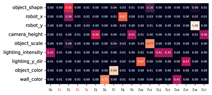
Tripod

Naive Tripod

Figure 5: Qualitative study of Tripod and naive Tripod on Isaac3D. Decoded latent interventions (top): in each column, we encode an image and visualize the effect of intervening on a single latent on decoding by varying its value in a linear interpolation in that latent’s range. Normalized mutual information heatmaps (bottom): this acts as an “answer key” to what the observed qualitative changes in a column should be when considering the entire dataset. Red latents are inactive and corresponding columns are removed from the latent intervention visualizations. For more qualitative results, see Appendix C.

Comparison of Tripod with $\beta$-TCVAE, QLAE, and naive Tripod. Tripod outperforms $\beta$-TCVAE in both modularity metrics (InfoM and D), the DCI compactness metric C, and both explicitness metrics (InfoE and I). The total correlation regularization in $\beta$-TCVAE is analogous to the kernel-based latent multiinformation (KLM) regularization in Tripod; since this directly optimizes for compactness, it is no surprise that the two methods are competitive in InfoC. However, the substantial difference in InfoE indicates that the sources are more linearly predictable from Tripod latents than $\beta$-TCVAE latents.

In contrast, Tripod handidly outperforms QLAE in all modularity and compactness metrics while achieving parity in both explicitness metrics. This suggests that latent quantization, a property common to both methods, is important to achieve high explicitness. The difference in modularity and compactness is explained by the lack of the other two inductive biases, KLM and NHP, in QLAE.

Tripod dominates naive Tripod on every disentanglement metric for each dataset. This validates the utility of our technical contributions. Indeed, naive Tripod is virtually indistinguishable from QLAE in aggregate, demonstrating that our specific modifications to the three inductive biases are necessary to achieve a synergistic disentangling effect. We highlight that the marked difference in compactness (InfoC and C in Table 3.4, row sparsity in normalized mutual information heatmaps of Figure 5) reflects naive Tripod’s reluctance to deactivate latents due to its vanilla Hessian penalty leg: shrinking latents increases the curvature of the decoder. In contrast, the invariance to latent scaling built into Tripod’s NHP leg enables latent deactivation.

Ablation studies on Tripod. We ablate each leg of Tripod in turn. We take the exact configuration we use for each dataset and either set the corresponding regularization weight to $0$ for ablating NHP or KLM, or change the number of quantized values from $12$ to $12^{2}$ for ablating FSQ. Tripod w/o NHP takes a significant hit in all modularity and compactness metrics, concretely demonstrating a beneficial application of the Hessian penalty to autoencoders for the first time. Tripod w/o KLM suffers a slightly cushioned blow in the same metrics. Interestingly, Tripod w/ finer quantization incurs the most significant penalty, suggesting that the enforced compression and latent organization afforded by finite scalar quantization underpins Tripod.

4.3 Qualitative Results

For each dataset, we qualitatively compare Tripod and naive Tripod in terms of how they decode under latent interventions. For reference, we also visualize the pairwise mutual information heatmap between sources and latents (from which the InfoM and InfoC metrics are calculated). Figure 5 presents this for Isaac3D. Due to space constraints, the rest of this material can be found in Appendix C. We find that the quantitative improvement of Tripod over naive Tripod is mirrored in how consistently intervening on a particular latent dimension affects generation.

5 Related Work

Disentanglement and identifiability. The classic problem of independent components analysis (ICA; Comon (1994); Hyvärinen & Oja (2000)) can be viewed as the progenitor of disentangled representation learning. Notoriously, disentanglement is theoretically underspecified (Hyvärinen & Oja, 2000; Locatello et al., 2019) when the data-generating process is nonlinear (Hyvärinen & Pajunen, 1999), so disentangling in practice relies heavily on inductive biases.

Architectural inductive biases for disentanglement. We build on the architectural inductive bias of latent quantization (Hsu et al., 2023). Leeb et al. (2023) demonstrate that restricting different latents to enter the decoding computation graph at different points can enable disentanglement. We view this as specifying a rather specific structure for the latent space (essentially assuming one source variable per hierarchy level) and opt not to use it.

Disentanglement via regularizing autoencoders. Our work follows in the tradition of applying regularizations on autoencoder architectures to encourage disentanglement. Specifically, the KLM regularization falls into an information-theoretic family of regularization techniques. The simplest example of this is the $\beta$-VAE (Higgins et al., 2017), which places a heavier weight on the KL-divergence term in the VAE evidence lower bound. To curb the trade-off between disentanglement and reconstruction, Burgess et al. (2017) modify $\beta$-VAE to increase the information capacity of latent representations during training. Chen et al. (2018) identify a decomposition of the KL-divergence into $3$ terms and argue that only the total correlation term has a disentangling effect; their proposed model, $\beta$-TCVAE, upweights only this term. Similarly, Kim & Mnih (2018) also regularize latent multiinformation, but use an auxiliary discriminator and the density-ratio trick to estimate multiinformation. We opt not to use this method due to the unwieldy auxiliary discriminator. Kumar et al. (2018) investigate a more thorough optimization of the KL-divergence through moment matching. Whittington et al. (2023) show that biologically-inspired constraints that minimize latent activity and weight energy while promoting latent non-negativity help models learn disentangled representations.

Functional inductive biases on the learned data-generating mapping. Tripod also incorporates a functional inductive bias on the latent-to-data mapping. Peebles et al. (2020) and Wei et al. (2021) propose regularizing the derivatives of a GAN’s generator to minimize inter-latent dependencies. While the former focuses on the mixed derivatives (off-diagonal elements of the Hessian), the latter regularizes the columns of the Jacobian to be orthogonal. Similarly, Gresele et al. (2021) mathematically show how a Jacobian column orthogonality criterion can rule out classic indeterminancies in nonlinear independent components analysis. We find the vanishing mixed derivative criterion more conceptually appealing, especially since near-orthgonality becomes trivial in high-dimensional activation and data spaces. In a separate vein, Sorrenson et al. (2020) and Yang et al. (2022) investigate the assumption of volume preservation in data generation. Finally, sparsity has seen considerable attention in works pursuing identifiability (Jing et al., 2020; Zheng et al., 2022; Moran et al., 2022).

6 Discussion

In this work, we meld three previously proposed ideas for disentanglement into Tripod, a method that makes necessary modifications to existing instantiations of these ideas so that a synergy between the components is realized in practice. These conceptual and technical contributions are validated in our experiments: both the specific set of three inductive biases as well as our modifications are essential to Tripod’s performance. However, one trade-off is an increased computational footprint due to the use of multiple inductive biases in Tripod. A profiling study (Appendix D) indicates that FSQ and KLM incur negligible overhead, but NHP increases training iteration runtime by a factor of about $2.5$ due to the extra decoder forward passes required for its regularization term.

Given the sensitivity of Tripod to the degree of quantization (i.e., of compression) identified in our ablation study, it may be fruitful to study mechanisms to automatically tune or learn this key (hyper)parameter. Naturally, this would need to be unsupervised or highly label-efficient in order to be practically useful. One potential unsupervised tuning procedure would be to begin with a channel capacity that is too low, and to increase it until reconstruction performance starts saturating. The key assumption here is that the true sources are an optimal or near-optimal compression of the data. For the label-efficient setting, it may well be good enough to simply use disentanglement metrics such as InfoMEC. The fixed latent space bounds and lack of learnable codes in our FSQ implementation also enable on-the-fly adaptation of the degree of quantization.

Our empirical evaluation is limited to image datasets because this is the only modality (beyond toy low-dimensional setups) we are aware of for which there exist datasets that (i) obey the nonlinear ICA data generation assumptions and (ii) enable quantitative evaluation via ground-truth source labels that completely explain the data. A priori, we expect Tripod, instantiated with appropriate architectures, to also be effective for other modalities, e.g. time series or graphs, as no assumptions specific to images are made in the formulation of any of the three Tripod legs.

Finally, our work demonstrates that a feasible alternative to racking our brains in search of new inductive biases for disentanglement is to revisit previously proposed ideas and refurbish them for use in tandem. Indeed, it may be that the right set of component techniques for disentanglement already exist and are simply waiting to be put together.

Acknowledgements

We gratefully acknowledge the developers of open-source software packages that facilitated this research: NumPy (Harris et al., 2020), JAX (Bradbury et al., 2018), Equinox (Kidger & Garcia, 2021), and scikit-learn (Pedregosa et al., 2011). We also thank Will Dorrell, Stefano Ermon, Yoonho Lee, Allan Zhou, Asher Spector, and anonymous reviewers for helpful discussions and feedback on previous drafts. KH was funded by a Sequoia Capital Stanford Graduate Fellowship. This research was also supported by ONR grants N00014-22-1-2621 and MURI N00014-22-1-2740.

Broader Impact Statement

We view the problem of disentanglement as a manifestation of the desire to have machine learning models experience the world as we humans do. We are thus optimistic that this work and others like it will have a role to play in empowering human decision-making in a world increasingly permeated with such models. Nevertheless, like many other AI technologies, disentanglement has potential negative impacts. Examples include enhanced disinformation dissemination, more invasive personal profiling from behavioral data, and increased automation of sensitive decision-making. Avenues for mitigating such negative outcomes include technical approaches, e.g. using human-in-the-loop rather than fully automated systems, as well as policy considerations, e.g. regulation guidelines for the appropriate deployment of models. Proactive pursuit of such strategies may well be crucial for ensuring the positive broader impact of disentanglement.

Appendix A Proofs

A.1 Proof of Proposition 3.1

Proposition 3.1. The Hessian penalty

$$\sum_{j_{1}\neq j_{2}}\left(H^{[k]}_{j_{1}j_{2}}\right)^{2}$$ (18)

can be reduced by scaling down $\hat{g}^{[k]}$ or scaling up any $z_{j},j\in[{n_{z}}]$, and vice versa. In contrast, the normalized Hessian penalty

$$\frac{\sum_{j_{1}\neq j_{2}}\left(H^{[k]}_{j_{1}j_{2}}\sigma_{j_{1}}\sigma_{j_{2}}\right)^{2}}{\sum_{j_{1},j_{2}}\left(H^{[k]}_{j_{1}j_{2}}\sigma_{j_{1}}\sigma_{j_{2}}\right)^{2}}$$ (19)

is invariant to the scaling of ${\hat{g}}^{[k]}$ and $z_{j}\ \forall j\in[{n_{z}}]$.

Proof.

First, we prove the statement about the original Hessian penalty. Let $s\in(0,1)$. Then, if $\hat{g}^{\prime[k]}=s\hat{g}^{[k]}$,

$$\sum_{j_{1}\neq j_{2}}\left(H^{\prime[k]}_{j_{1}j_{2}}\right)^{2}=\sum_{j_{1}\neq j_{2}}\left(\frac{\partial}{\partial z_{j_{1}}}\frac{\partial\hat{g}^{\prime[k]}}{\partial z_{j_{2}}}\right)^{2}=\sum_{j_{1}\neq j_{2}}\left(\frac{\partial}{\partial z_{j_{1}}}\frac{\partial\hat{g}^{\prime[k]}}{\partial\hat{g}^{[k]}}\frac{\partial\hat{g}^{[k]}}{\partial z_{j_{2}}}\right)^{2}=\sum_{j_{1}\neq j_{2}}\left(\frac{\partial}{\partial z_{j_{1}}}\frac{\partial\hat{g}^{[k]}}{\partial z_{j_{2}}}\right)^{2}s^{2}<\sum_{j_{1}\neq j_{2}}\left(H^{[k]}_{j_{1}j_{2}}\right)^{2}.$$

Similarly, if $z_{i}^{\prime}=s_{i}z_{i}$ with $s_{i}\geq 1$ and $s_{l}>1$ for at least one $l\in[n_{z}]$, then

$$\sum_{j_{1}\neq j_{2}}\left(H^{\prime[k]}_{j_{1}j_{2}}\right)^{2}=\sum_{j_{1}\neq j_{2}}\left(\frac{\partial}{\partial z_{j_{1}}^{\prime}}\frac{\partial\hat{g}^{[k]}}{\partial z_{j_{2}}^{\prime}}\right)^{2}=\sum_{j_{1}\neq j_{2}}\left(\frac{\partial}{\partial z_{j_{1}}}\frac{\partial z_{j_{1}}}{\partial z_{j_{1}}^{\prime}}\frac{\partial\hat{g}^{[k]}}{\partial z_{j_{2}}}\frac{\partial z_{j_{2}}}{\partial z_{j_{2}}^{\prime}}\right)^{2}=\sum_{j_{1}\neq j_{2}}\left(\frac{\partial}{\partial z_{j_{1}}}\frac{\partial\hat{g}^{[k]}}{\partial z_{j_{2}}}\frac{1}{s_{j_{1}}s_{j_{2}}}\right)^{2}<\sum_{j_{1}\neq j_{2}}\left(H^{[k]}_{j_{1}j_{2}}\right)^{2}.$$

To show that the normalized Hessian penalty is invariant to scaling of $\hat{g}^{[k]}$, suppose we scale $\hat{g}^{[k]}$ to be $\hat{g}^{\prime[k]}=\alpha\hat{g}^{[k]}$. Then, the numerator becomes

$$\sum_{j_{1}\neq j_{2}}\left(H^{\prime[k]}_{j_{1}j_{2}}\sigma_{j_{1}}\sigma_{j_{2}}\right)^{2}=\sum_{j_{1}\neq j_{2}}\left(\frac{\partial}{\partial z_{j_{1}}}\frac{\partial\hat{g}^{\prime[k]}}{\partial z_{j_{2}}}\sigma_{j_{1}}\sigma_{j_{2}}\right)^{2}=\sum_{j_{1}\neq j_{2}}\left(\frac{\partial}{\partial z_{j_{1}}}\frac{\partial\hat{g}^{\prime[k]}}{\partial\hat{g}^{[k]}}\frac{\partial\hat{g}^{[k]}}{\partial z_{j_{2}}}\sigma_{j_{1}}\sigma_{j_{2}}\right)^{2}=\alpha^{2}\sum_{j_{1}\neq j_{2}}\left(H^{[k]}_{j_{1}j_{2}}\sigma_{j_{1}}\sigma_{j_{2}}\right)^{2}.$$

Similarly, the denominator becomes $\sum_{j_{1},j_{2}}\left(H^{\prime[k]}_{j_{1}j_{2}}\sigma_{j_{1}}\sigma_{j_{2}}\right)^{2}=\alpha^{2}\sum_{j_{1},j_{2}}\left(H^{[k]}_{j_{1}j_{2}}\sigma_{j_{1}}\sigma_{j_{2}}\right)^{2}$, allowing us to write

$$\frac{\sum_{j_{1}\neq j_{2}}\left(H^{\prime[k]}_{j_{1}j_{2}}\sigma_{j_{1}}\sigma_{j_{2}}\right)^{2}}{\sum_{j_{1},j_{2}}\left(H^{\prime[k]}_{j_{1}j_{2}}\sigma_{j_{1}}\sigma_{j_{2}}\right)^{2}}=\frac{\sum_{j_{1}\neq j_{2}}\left(H^{[k]}_{j_{1}j_{2}}\sigma_{j_{1}}\sigma_{j_{2}}\right)^{2}}{\sum_{j_{1},j_{2}}\left(H^{[k]}_{j_{1}j_{2}}\sigma_{j_{1}}\sigma_{j_{2}}\right)^{2}}$$

Now, we verify that the normalized Hessian penalty is invariant to any scaling of the inputs. If $z_{j_{1}}$ is scaled by $s_{1}$ so that $z_{j_{1}}^{\prime}=s_{1}z_{j_{1}}$ and $z_{j_{2}}$ is scaled by $s_{2}$ so that $z_{j_{2}}^{\prime}=s_{2}z_{j_{2}}$, then each term (in both the numerator and the denominator) becomes

$$\left(H^{\prime[k]}_{j_{1}j_{2}}\sigma_{j_{1}}^{\prime}\sigma_{j_{2}}^{\prime}\right)^{2} =\left(\frac{\partial}{\partial z_{j_{1}}^{\prime}}\frac{\partial\hat{g}^{[k]}}{\partial z_{j_{2}}^{\prime}}\sigma_{j_{1}}^{\prime}\sigma_{j_{2}}^{\prime}\right)^{2}$$

$$=\left(\frac{\partial}{\partial z_{j_{1}}}\frac{\partial z_{j_{1}}}{\partial z_{j_{1}}^{\prime}}\left(\frac{\partial\hat{g}^{[k]}}{\partial z_{j_{2}}}\frac{\partial z_{j_{2}}}{\partial z_{j_{2}}^{\prime}}\right)\sigma_{j_{1}}^{\prime}\sigma_{j_{2}}^{\prime}\right)^{2}$$

$$=\left(\frac{1}{s_{1}}\frac{\partial}{\partial z_{j_{1}}}\left(\frac{1}{s_{2}}\frac{\partial\hat{g}^{[k]}}{\partial z_{j_{2}}}\right)s_{1}\sigma_{j_{1}}s_{2}\sigma_{j_{2}}\right)^{2}$$

$$=\left(\frac{\partial}{\partial z_{j_{1}}}\frac{\partial\hat{g}^{[k]}}{\partial z_{j_{2}}}\sigma_{j_{1}}\sigma_{j_{2}}\right)^{2}$$

$$=\left(H^{[k]}_{j_{1}j_{2}}\sigma_{j_{1}}\sigma_{j_{2}}\right)^{2},$$

and the normalized Hessian penalty remains invariant. ∎

A.2 Proof of Proposition 3.2

Proposition 3.2. Let $v$ and $w$ be random vectors where $v_{j}\sim\operatorname{Rademacher}(\sigma_{j})$ and $w_{j}\sim\mathcal{N}(0,\sigma_{j}^{2})$. Then the normalized Hessian penalty can be computed as

$$\frac{\sum_{j_{1}\neq j_{2}}\left(H^{[k]}_{j_{1}j_{2}}\sigma_{j_{1}}\sigma_{j_{2}}\right)^{2}}{\sum_{j_{1},j_{2}}\left(H^{[k]}_{j_{1}j_{2}}\sigma_{j_{1}}\sigma_{j_{2}}\right)^{2}}=\frac{\operatorname*{Var}\left[v^{T}H^{[k]}v\right]}{\operatorname*{Var}\left[w^{T}H^{[k]}w\right]}.$$ (20)

Proof.

For the numerator, we first write $\operatorname*{Var}\left[v^{\top}H^{[k]}v\right]=\operatorname*{Var}\left[v^{\top}H^{[k]}v-\mathbb{E}\left[v^{\top}H^{[k]}v\right]\right]$. Now,

$$v^{\top}H^{[k]}v-\mathbb{E}\left[v^{\top}H^{[k]}v\right] =\sum_{j_{1},j_{2}}v_{j_{1}}H^{[k]}_{j_{1}j_{2}}v_{j_{2}}-\mathbb{E}\left[v^{\top}H^{[k]}v\right]$$

$$=\sum_{j_{1},j_{2}}v_{j_{1}}H^{[k]}_{j_{1}j_{2}}v_{j_{2}}-\mathbb{E}\left[\operatorname{Tr}\left(v^{\top}H^{[k]}v\right)\right]$$

$$=\sum_{j_{1},j_{2}}v_{j_{1}}H^{[k]}_{j_{1}j_{2}}v_{j_{2}}-\mathbb{E}\left[\operatorname{Tr}\left(H^{[k]}vv^{T}\right)\right]$$

$$=\sum_{j_{1},j_{2}}v_{j_{1}}H^{[k]}_{j_{1}j_{2}}v_{j_{2}}-\operatorname{Tr}\left(H^{[k]}\mathbb{E}\left[vv^{T}\right]\right)$$

$$=\sum_{j_{1},j_{2}}v_{j_{1}}H^{[k]}_{j_{1}j_{2}}v_{j_{2}}-\sum_{j}H^{[k]}_{jj}\sigma_{j}^{2}$$

$$=\sum_{j_{1},j_{2}}v_{j_{1}}H^{[k]}_{j_{1}j_{2}}v_{j_{2}}-\sum_{j}H^{[k]}_{jj}v_{j}^{2}+\sum_{j}H^{[k]}_{jj}v_{j}^{2}-\sum_{j}H^{[k]}_{jj}\sigma_{j}^{2}$$

$$=\sum_{j_{1}\neq j_{2}}v_{j_{1}}H^{[k]}_{j_{1}j_{2}}v_{j_{2}}+\sum_{j}H^{[k]}_{jj}(v_{j}^{2}-\sigma_{j}^{2})$$

$$=\sum_{j_{1}\neq j_{2}}v_{j_{1}}H^{[k]}_{j_{1}j_{2}}v_{j_{2}}+\sum_{j}H^{[k]}_{jj}(\sigma_{j}^{2}-\sigma_{j}^{2})\qquad\because v_{j}\sim\operatorname{Rademacher}(\sigma_{j})$$

$$=\sum_{j_{1}\neq j_{2}}v_{j_{1}}H^{[k]}_{j_{1}j_{2}}v_{j_{2}}$$

Taking the variance, we have:

$$\operatorname*{Var}\left[\sum_{j_{1}\neq j_{2}}v_{j_{1}}H^{[k]}_{j_{1}j_{2}}v_{j_{2}}\right] =\operatorname*{Var}\left[2\sum_{j_{1}>j_{2}}v_{j_{1}}H^{[k]}_{j_{1}j_{2}}v_{j_{2}}\right] \because H^{[k]}\text{ is symmetric}$$

$$=4\sum_{j_{1}>j_{2}}\left(H^{[k]}_{j_{1}j_{2}}\right)^{2}\operatorname*{Var}\left[v_{j_{1}}v_{j_{2}}\right]$$

$$=4\sum_{j_{1}>j_{2}}\left(H^{[k]}_{j_{1}j_{2}}\right)^{2}\sigma_{j_{1}}^{2}\sigma_{j_{2}}^{2}$$

$$=2\sum_{j_{1}\neq j_{2}}\left(H^{[k]}_{j_{1}j_{2}}\sigma_{j_{1}}\sigma_{j_{2}}\right)^{2} \because H^{[k]}\text{ is symmetric}$$

For the denominator, we have

$$\operatorname*{Var}\left[w^{\top}H^{[k]}w\right] =\operatorname*{Var}\left[\sum_{j_{1}\neq j_{2}}w_{j_{1}}H^{[k]}_{j_{1}j_{2}}w_{j_{2}}+\sum_{j}w_{j}^{2}H^{[k]}_{jj}\right]$$

$$=\operatorname*{Var}\left[\sum_{j_{1}}\left(2\sum_{j_{1}>j_{2}}w_{j_{1}}H^{[k]}_{j_{1}j_{2}}w_{j_{2}}+w_{j_{1}}^{2}H^{[k]}_{j_{1}j_{1}}\right)\right]$$

$$=\sum_{j_{1}}\operatorname*{Var}\left[\left(2\sum_{j_{1}>j_{2}}w_{j_{1}}H^{[k]}_{j_{1}j_{2}}w_{j_{2}}+w_{j_{1}}^{2}H^{[k]}_{j_{1}j_{1}}\right)\right]$$

$$+\sum_{j_{1}\neq j_{1}^{\prime}}\mathrm{Cov}\left(\left(2\sum_{j_{1}>j_{2}}w_{j_{1}}H^{[k]}_{j_{1}j_{2}}w_{j_{2}}+w_{j_{1}}^{2}H^{[k]}_{j_{1}j_{1}}\right),\left(2\sum_{j_{1}^{\prime}>j_{2}^{\prime}}w_{j_{1}^{\prime}}H^{[k]}_{j_{1}^{\prime}j_{2}^{\prime}}w_{j_{2}^{\prime}}+w_{j_{1}^{\prime}}^{2}H^{[k]}_{j_{1}^{\prime}j_{1}^{\prime}}\right)\right)$$

The covariance terms vanish. To see this, note that

$$\mathrm{Cov}\left(w_{j_{1}}H^{[k]}_{j_{1}j_{2}}w_{j_{2}},w_{j_{1}^{\prime}}H^{[k]}_{j_{1}^{\prime}j_{2}^{\prime}}w_{j_{2}^{\prime}}\right) =\mathbb{E}\left[w_{j_{1}}H^{[k]}_{j_{1}j_{2}}w_{j_{2}}w_{j_{1}^{\prime}}H^{[k]}_{j_{1}^{\prime}j_{2}^{\prime}}w_{j_{2}^{\prime}}\right]-\mathbb{E}\left[w_{j_{1}}H^{[k]}_{j_{1}j_{2}}w_{j_{2}}\right]\mathbb{E}\left[w_{j_{1}^{\prime}}H^{[k]}_{j_{1}^{\prime}j_{2}^{\prime}}w_{j_{2}^{\prime}}\right]$$

$$=\mathbb{E}\left[w_{j_{1}}\right]\mathbb{E}\left[H^{[k]}_{j_{1}j_{2}}w_{j_{2}}w_{j_{1}^{\prime}}H^{[k]}_{j_{1}^{\prime}j_{2}^{\prime}}w_{j_{2}^{\prime}}\right]-\mathbb{E}\left[w_{j_{1}}\right]\mathbb{E}\left[H^{[k]}_{j_{1}j_{2}}w_{j_{2}}\right]\mathbb{E}\left[w_{j_{1}^{\prime}}\right]\mathbb{E}\left[H^{[k]}_{j_{1}^{\prime}j_{2}^{\prime}}w_{j_{2}^{\prime}}\right]$$

$$=0,$$

where we leverage that either $j_{1}\neq j^{\prime}_{2}$ or $j_{2}\neq j_{1}^{\prime}$ must hold else the two terms are identical, and write the case of the former without loss of generality. Similarly,

$$\mathrm{Cov}\left(w_{j_{1}}H^{[k]}_{j_{1}j_{2}}w_{j_{2}},w_{j_{1}^{\prime}}^{2}H^{[k]}_{j_{1}^{\prime}j_{1}^{\prime}}\right)=\mathrm{Cov}\left(w_{j_{1}}H^{[k]}_{j_{1}j_{2}}w_{j_{2}},w_{j_{1}}^{2}H^{[k]}_{j_{1}j_{1}}\right)=0$$

since in each of these expressions there is at least one normal variable independent of all other variables that has not been raised to a power greater than 1. Lastly,

$$\mathrm{Cov}\left(w_{j_{1}}^{2}H^{[k]}_{j_{1}j_{1}},w_{j_{1}^{\prime}}^{2}H^{[k]}_{j_{1}^{\prime}j_{1}^{\prime}}\right) =\mathbb{E}\left[w_{j_{1}}^{2}H^{[k]}_{j_{1}j_{1}}w_{j_{1}^{\prime}}^{2}H^{[k]}_{j_{1}^{\prime}j_{1}^{\prime}}\right]-\mathbb{E}\left[w_{j_{1}^{\prime}}^{2}H^{[k]}_{j_{1}^{\prime}j_{1}^{\prime}}\right]\mathbb{E}\left[w_{j_{1}}^{2}H^{[k]}_{j_{1}j_{1}}\right]$$

$$=H^{[k]}_{j_{1}j_{1}}H^{[k]}_{j_{1}^{\prime}j_{1}^{\prime}}\sigma_{j_{1}}^{2}\sigma_{j_{1}^{\prime}}^{2}-H^{[k]}_{j_{1}j_{1}}H^{[k]}_{j_{1}^{\prime}j_{1}^{\prime}}\sigma_{j_{1}}^{2}\sigma_{j_{1}^{\prime}}^{2}$$

$$=0.$$

Since the covariance terms vanish, we have

$$\operatorname*{Var}\left[w^{\top}H^{[k]}w\right] =\operatorname*{Var}\left[\sum_{j_{1}}\left(2\sum_{j_{1}>j_{2}}w_{j_{1}}H^{[k]}_{j_{1}j_{2}}w_{j_{2}}+w_{j_{1}}^{2}H^{[k]}_{j_{1}j_{1}}\right)\right]$$

$$=\sum_{j_{1}}\operatorname*{Var}\left[2\sum_{j_{1}>j_{2}}w_{j_{1}}H^{[k]}_{j_{1}j_{2}}w_{j_{2}}+w_{j_{1}}^{2}H^{[k]}_{j_{1}j_{1}}\right].$$

Now, we expand:

$$\sum_{j_{1}}\left(\operatorname*{Var}\left[2\sum_{j_{1}>j_{2}}w_{j_{1}}H^{[k]}_{j_{1}j_{2}}w_{j_{2}}+w_{j_{1}}^{2}H^{[k]}_{j_{1}j_{1}}\right]\right)$$

$$= \sum_{j_{1}}\left(\operatorname*{Var}\left[2\sum_{j_{1}>j_{2}}w_{j_{1}}H^{[k]}_{j_{1}j_{2}}w_{j_{2}}\right]+\operatorname*{Var}\left[w_{j_{1}}^{2}H^{[k]}_{j_{1}j_{1}}\right]+2\mathrm{Cov}\left(2\sum_{j_{1}>j_{2}}w_{j_{1}}H^{[k]}_{jj}w_{j_{2}},w_{j_{1}}^{2}H^{[k]}_{j_{1}j_{1}}\right)\right).$$

However, for all $j_{1}$,

$$2\mathrm{Cov}\left(2\sum_{j_{1}>j_{2}}w_{j_{1}}H^{[k]}_{jj}w_{j_{2}},w_{j_{1}}^{2}H^{[k]}_{j_{1}j_{1}}\right) =\mathbb{E}\left[2w_{j_{1}}^{3}H^{[k]}_{j_{1}j_{1}}\sum_{j_{1}>j_{2}}H^{[k]}_{j_{1}j_{2}}w_{j_{2}}\right]-\mathbb{E}\left[2w_{j_{1}}\sum_{j_{1}>j_{2}}H^{[k]}_{j_{1}j_{2}}w_{j_{2}}\right]\mathbb{E}\left[w_{j_{1}}^{2}H^{[k]}_{j_{1}j_{1}}\right]$$

$$=2H^{[k]}_{j_{1}j_{1}}\sum_{j_{1}>j_{2}}H^{[k]}_{j_{1}j_{2}}\mathbb{E}\left[w_{j_{1}}^{3}w_{j_{2}}\right]-2H^{[k]}_{j_{1}j_{1}}\sum_{j_{1}>j_{2}}H^{[k]}_{j_{1}j_{2}}\mathbb{E}\left[w_{j_{1}}w_{j_{2}}\right]\mathbb{E}\left[w_{j_{1}}^{2}\right]$$

$$=2H^{[k]}_{j_{1}j_{1}}\sum_{j_{1}>j_{2}}H^{[k]}_{j_{1}j_{2}}\mathbb{E}\left[w_{j_{1}}^{3}\right]\mathbb{E}\left[w_{j_{2}}\right]-2H^{[k]}_{j_{1}j_{1}}\sum_{j_{1}>j_{2}}H^{[k]}_{j_{1}j_{2}}\mathbb{E}\left[w_{j_{1}}\right]\mathbb{E}\left[w_{j_{2}}\right]\mathbb{E}\left[w_{j_{1}}^{2}\right]$$

$$=0.$$

Therefore,

$$\operatorname*{Var}\left[w^{\top}H^{[k]}w\right] =\sum_{j_{1}}\left(\operatorname*{Var}\left[2\sum_{j_{1}>j_{2}}w_{j_{1}}H^{[k]}_{j_{1}j_{2}}w_{j_{2}}\right]+\operatorname*{Var}\left[w_{j_{1}}^{2}H^{[k]}_{j_{1}j_{1}}\right]\right)$$

$$=\sum_{j_{1}}\left(4\sum_{j_{1}>j_{2}}\left(H^{[k]}_{j_{1}j_{2}}\right)^{2}\operatorname*{Var}\left[w_{j_{1}}w_{j_{2}}\right]+\left(H^{[k]}_{j_{1}j_{1}}\right)^{2}\operatorname*{Var}\left[w_{j_{1}}^{2}\right]\right)$$

$$=\sum_{j_{1}}\left(4\sum_{j_{1}>j_{2}}\left(H^{[k]}_{j_{1}j_{2}}\right)^{2}\sigma_{j_{1}}^{2}\sigma_{j_{1}}^{2}+2\left(H^{[k]}_{jj}\right)^{2}\sigma_{j_{1}}^{2}\right)$$

$$=2\sum_{j_{1},j_{2}}\left(H^{[k]}_{j_{1}j_{2}}\right)^{2}\sigma_{j_{1}}^{2}\sigma_{j}^{2}$$

where we used the fact that the variance of product of two independent normal variables centered at 0 is the product of their variances and the variance of the square of a normal variable is twice its variance squared.

Taking the simplified forms of the numerator and denominator, we obtain

$$\frac{\operatorname*{Var}\left[v^{\top}H^{[k]}v\right]}{\operatorname*{Var}\left[w^{\top}H^{[k]}w\right]} =\frac{2\sum_{j_{1}\neq j_{2}}\left(H^{[k]}_{j_{1}j_{2}}\sigma_{j_{1}}\sigma_{j_{2}}\right)^{2}}{2\sum_{j_{1},j_{2}}\left(H^{[k]}_{j_{1}j_{2}}\sigma_{j_{1}}\sigma_{j_{2}}\right)^{2}}=\frac{\sum_{j_{1}\neq j_{2}}\left(H^{[k]}_{j_{1}j_{2}}\sigma_{j_{1}}\sigma_{j_{2}}\right)^{2}}{\sum_{j_{1},j_{2}}\left(H^{[k]}_{j_{1}j_{2}}\sigma_{j_{1}}\sigma_{j_{2}}\right)^{2}}$$

∎

Appendix B Experimental Details

This section contains details on the experiments conducted in this work.

B.1 Datasets

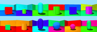
(a) Shapes3D

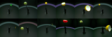
(b) MPI3D

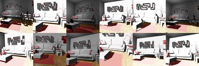
(c) Falcor3D

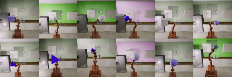
(d) Isaac3D

Figure 6: Random data samples from each dataset.

Table 2: Summary of datasets used for empirical evaluation.

dataset	${n_{s}}$	$|\mathcal{D}|$	PSNR threshold (dB) for $64\times 64$
Shapes3D (Burgess & Kim, 2018)	$6$	$480000$	38
MPI3D (Gondal et al., 2019)	$7$	$460800$	42
Falcor3D (Nie, 2019)	$7$	$233280$	34
Isaac3D (Nie, 2019)	$9$	$737280$	40

Table 3: Dataset sources.

	Shapes3D		MPI3D		Falcor3D		Isaac3D
index	description	values	description	values	description	values	description	values
0	floor color	10	object color	4	lighting intensity	5	object shape	3
1	object color	10	object shape	4	lighting x	6	robot x	8
2	camera orientation	10	object size	2	lighting y	6	robot y	5
3	object scale	8	camera height	3	lighting z	6	camera height	4
4	object shape	4	background color	3	camera x	6	object scale	4
5	wall color	15	robot x	40	camera y	6	lighting intensity	4
6			robot y	40	camera z	6	lighting direction	6
7							object color	4
8							wall color	4

B.2 Hyperparameters

This section specifies fixed and tuned hyperparameters for all methods considered.

Table 4: Fixed hyperparameters for all autoencoder variants.

hyperparameter	value
number of latents $n_{z}$	$2{n_{s}}$
AdamW learning rate	${1\times 10^{-3}}$
AdamW $\beta_{1}$	$0.9$
AdamW $\beta_{2}$	$0.99$
AdamW updates	$\leq 2\times 10^{5}$
batch size	64

Table 5: Key regularization hyperparameter tuning done for each autoencoder

method	hyperparameter	values
$\beta$-TCVAE	$\beta=\lambda_{\text{total correlation}}$	$[1,2,3,5,10]$
QLAE	weight decay	$[1\times 10^{-8},1\times 10^{-6},1\times 10^{-4},1\times 10^{-2},1]$
Tripod (naive)	$\lambda_{\text{vanilla Hessian penalty}}$	$[0,1\times 10^{-10},1\times 10^{-8},1\times 10^{-6},1\times 10^{-4},1\times 10^{-2}]$
Tripod (naive)	$\lambda_{\text{latent multiinformation}}$	$[0,1\times 10^{-10},1\times 10^{-8},1\times 10^{-6},1\times 10^{-4},1\times 10^{-2}]$
Tripod	$\lambda_{\text{NHP}}$	$[0,1\times 10^{-10},1\times 10^{-8},1\times 10^{-6},1\times 10^{-4},1\times 10^{-2}]$
Tripod	$\lambda_{\text{KLM}}$	$[0,1\times 10^{-10},1\times 10^{-8},1\times 10^{-6},1\times 10^{-4},1\times 10^{-2}]$

Appendix C Qualitative Results

We qualitatively compare Tripod and naive Tripod on each dataset. In each column, we encode an image and visualize the effect of intervening on a single latent on decoding by varying its value in a linear interpolation in that latent’s range. Below, we also provide a normalized mutual information heatmap that acts as an “answer key” to what the qualitative change in a column should be. Red latents are inactive and corresponding columns are removed from the latent intervention visualizations.

$z_{0}$

$z_{1}$

$z_{2}$

$z_{3}$

$z_{4}$

$z_{5}$

$z_{6}$

$z_{7}$

$z_{8}$

$z_{9}$

$z_{10}$

$z_{11}$

$z_{0}$

$z_{1}$

$z_{2}$

$z_{3}$

$z_{4}$

$z_{5}$

$z_{6}$

$z_{7}$

$z_{8}$

$z_{9}$

$z_{10}$

$z_{11}$

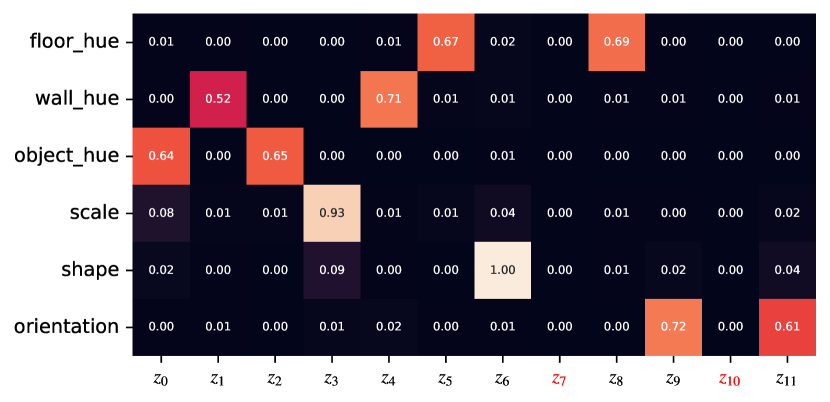
(a) Tripod

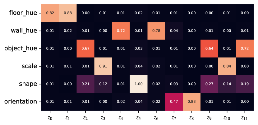
(b) Naive Tripod

Figure 7: Tripod and naive Tripod decoded latent interventions and normalized mutual information heatmaps on Shapes3D.

$z_{0}$

$z_{1}$

$z_{2}$

$z_{3}$

$z_{4}$

$z_{5}$

$z_{6}$

$z_{7}$

$z_{8}$

$z_{9}$

$z_{10}$

$z_{11}$

$z_{12}$

$z_{13}$

$z_{0}$

$z_{1}$

$z_{2}$

$z_{3}$

$z_{4}$

$z_{5}$

$z_{6}$

$z_{7}$

$z_{8}$

$z_{9}$

$z_{10}$

$z_{11}$

$z_{12}$

$z_{13}$

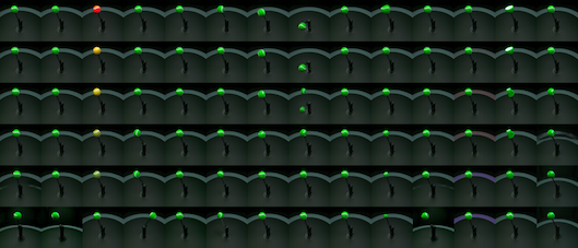
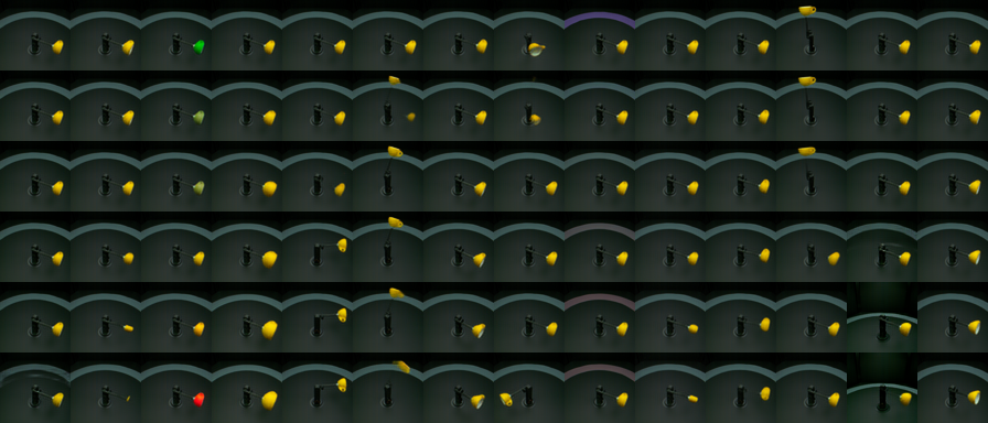
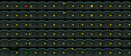
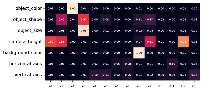
(a) Tripod

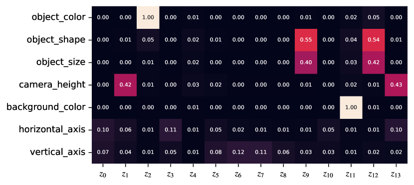
(b) Naive Tripod

Figure 8: Tripod and naive Tripod decoded latent interventions and normalized mutual information heatmaps on MPI3D.

$z_{0}$

$z_{1}$

$z_{2}$

$z_{3}$

$z_{4}$

$z_{5}$

$z_{6}$

$z_{7}$

$z_{8}$

$z_{9}$

$z_{10}$

$z_{11}$

$z_{12}$

$z_{13}$

$z_{0}$

$z_{1}$

$z_{2}$

$z_{3}$

$z_{4}$

$z_{5}$

$z_{6}$

$z_{7}$

$z_{8}$

$z_{9}$

$z_{10}$

$z_{11}$

$z_{12}$

$z_{13}$

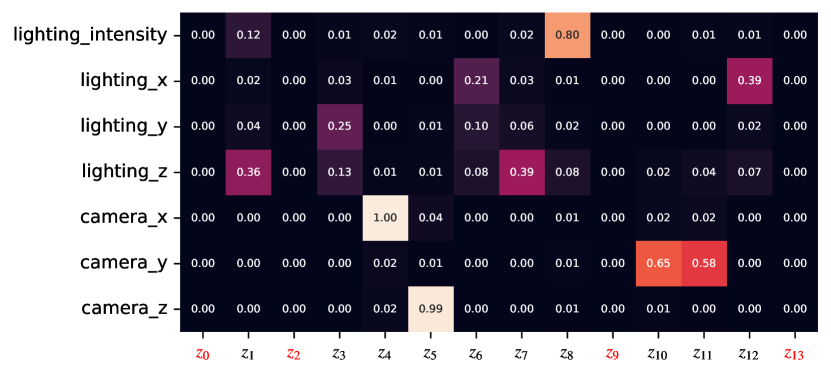
(a) Tripod

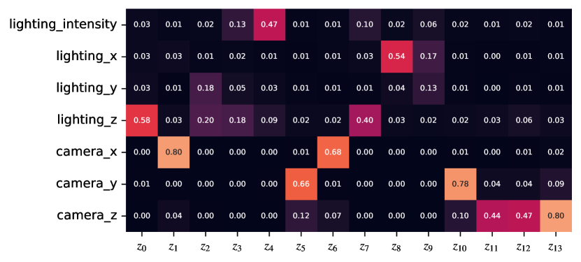
(b) Naive Tripod

Figure 9: Tripod and naive Tripod decoded latent interventions and normalized mutual information heatmaps on Falcor3D.

$z_{0}$

$z_{1}$

$z_{2}$

$z_{3}$

$z_{4}$

$z_{5}$

$z_{6}$

$z_{7}$

$z_{8}$

$z_{9}$

$z_{10}$

$z_{11}$

$z_{12}$

$z_{13}$

$z_{14}$

$z_{15}$

$z_{16}$

$z_{17}$

$z_{0}$

$z_{1}$

$z_{2}$

$z_{3}$

$z_{4}$

$z_{5}$

$z_{6}$

$z_{7}$

$z_{8}$

$z_{9}$

$z_{10}$

$z_{11}$

$z_{12}$

$z_{13}$

$z_{14}$

$z_{15}$

$z_{16}$

$z_{17}$

(a) Tripod

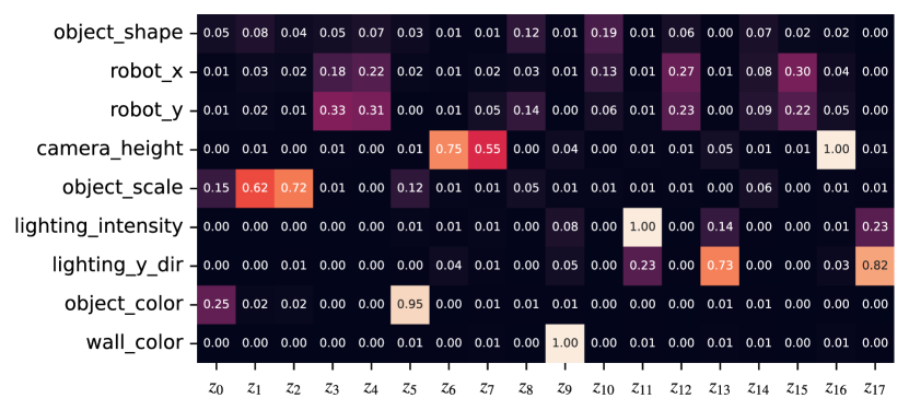
(b) Naive Tripod

Figure 10: Tripod and naive Tripod decoded latent interventions and normalized mutual information heatmaps on Isaac3D.

Appendix D Profiling Study

We measure the average time (in seconds) each training iteration takes for various models. We observe that latent quantization and kernel-based latent multiinformation incur minimal overhead. However, adding normalized Hessian penalty increases the runtime by a factor of about $2.5$ due to the extra forward passes required to compute its regularization term.

model	training iteration runtime (s)
$\beta$-TCVAE	0.040
QLAE	0.040
QLAE $+$ KLM	0.040
Tripod	0.106

Table 6: Profiling study results.

References

• Bengio (2013) Bengio, Y. Deep learning of representations: looking forward. In Statistical Language and Speech Processing, 2013.
• Bengio et al. (2013) Bengio, Y., Léonard, N., and Courville, A. Estimating or propagating gradients through stochastic neurons for conditional computation. arXiv preprint arXiv:1308.3432, 2013.
• Bradbury et al. (2018) Bradbury, J., Frostig, R., Hawkins, P., Johnson, M. J., Leary, C., Maclaurin, D., Necula, G., Paszke, A., VanderPlas, J., Wanderman-Milne, S., and Zhang, Q. JAX: composable transformations of Python+NumPy programs, 2018. URL http://github.com/google/jax.
• Burgess & Kim (2018) Burgess, C. and Kim, H. 3D shapes dataset, 2018. URL https://github.com/deepmind/3dshapes-dataset/.
• Burgess et al. (2017) Burgess, C. P., Higgins, I., Pal, A., Matthey, L., Watters, N., Desjardins, G., and Lerchner, A. Understanding disentangling in $\beta$-VAE. In NIPS Workshop on Learning Disentangled Representations, 2017.
• Chen et al. (2018) Chen, R. T., Li, X., Grosse, R. B., and Duvenaud, D. K. Isolating sources of disentanglement in variational autoencoders. In Advances in Neural Information Processing Systems, 2018.
• Comon (1994) Comon, P. Independent component analysis, a new concept? Signal Processing, 36(3):287–314, 1994.
• Dhariwal & Nichol (2021) Dhariwal, P. and Nichol, A. Diffusion models beat GANs on image synthesis. Advances in Neural Information Processing Systems, 2021.
• Eastwood & Williams (2018) Eastwood, C. and Williams, C. K. A framework for the quantitative evaluation of disentangled representations. In International Conference on Learning Representations, 2018.
• Gondal et al. (2019) Gondal, M. W., Wuthrich, M., Miladinovic, D., Locatello, F., Breidt, M., Volchkov, V., Akpo, J., Bachem, O., Schölkopf, B., and Bauer, S. On the transfer of inductive bias from simulation to the real world: a new disentanglement dataset. In Advances in Neural Information Processing Systems, 2019.
• Goodfellow et al. (2014) Goodfellow, I., Pouget-Abadie, J., Mirza, M., Xu, B., Warde-Farley, D., Ozair, S., Courville, A., and Bengio, Y. Generative adversarial networks. In Advances in Neural Information Processing Systems, 2014.
• Gresele et al. (2021) Gresele, L., Von Kügelgen, J., Stimper, V., Schölkopf, B., and Besserve, M. Independent mechanism analysis, a new concept? Advances in Neural Information Processing Systems, 2021.
• Harris et al. (2020) Harris, C. R., Millman, K. J., Van Der Walt, S. J., Gommers, R., Virtanen, P., Cournapeau, D., Wieser, E., Taylor, J., Berg, S., Smith, N. J., et al. Array programming with NumPy. Nature, 585(7825):357–362, 2020.
• Higgins et al. (2017) Higgins, I., Matthey, L., Pal, A., Burgess, C., Glorot, X., Botvinick, M., Mohamed, S., and Lerchner, A. $\beta$-VAE: learning basic visual concepts with a constrained variational framework. In International Conference on Learning Representations, 2017.
• Horan et al. (2021) Horan, D., Richardson, E., and Weiss, Y. When is unsupervised disentanglement possible? In Advances in Neural Information Processing Systems, 2021.
• Hsu et al. (2023) Hsu, K., Dorrell, W., Whittington, J. C., Wu, J., and Finn, C. Disentanglement via latent quantization. Advances in Neural Information Processing Systems, 2023.
• Hutchinson (1989) Hutchinson, M. F. A stochastic estimator of the trace of the influence matrix for laplacian smoothing splines. Communications in Statistics-Simulation and Computation, 18(3):1059–1076, 1989.
• Hyvärinen & Oja (2000) Hyvärinen, A. and Oja, E. Independent component analysis: algorithms and applications. Neural Networks, 13(4-5):411–430, 2000.
• Hyvärinen & Pajunen (1999) Hyvärinen, A. and Pajunen, P. Nonlinear independent component analysis: existence and uniqueness results. Neural Networks, 12(3):429–439, 1999.
• Jang et al. (2017) Jang, E., Gu, S., and Poole, B. Categorical reparameterization with Gumbel-Softmax. In International Conference on Learning Representations, 2017.
• Jing et al. (2020) Jing, L., Zbontar, J., et al. Implicit rank-minimizing autoencoder. In Advances in Neural Information Processing Systems, 2020.
• Khemakhem et al. (2020) Khemakhem, I., Kingma, D., Monti, R., and Hyvarinen, A. Variational autoencoders and nonlinear ICA: a unifying framework. In International Conference on Artificial Intelligence and Statistics, 2020.
• Kidger & Garcia (2021) Kidger, P. and Garcia, C. Equinox: neural networks in JAX via callable PyTrees and filtered transformations. Differentiable Programming Workshop at Neural Information Processing Systems, 2021.
• Kim & Mnih (2018) Kim, H. and Mnih, A. Disentangling by factorising. In International Conference on Machine Learning, 2018.
• Kingma & Welling (2014) Kingma, D. P. and Welling, M. Auto-encoding variational Bayes. In International Conference on Learning Representations, 2014.
• Kumar et al. (2018) Kumar, A., Sattigeri, P., and Balakrishnan, A. Variational inference of disentangled latent concepts from unlabeled observations. In International Conference on Learning Representations, 2018.
• Leeb et al. (2023) Leeb, F., Lanzillotta, G., Annadani, Y., Besserve, M., Bauer, S., and Schölkopf, B. Structure by architecture: structured representations without regularization. In International Conference on Learning Representations, 2023.
• Locatello et al. (2019) Locatello, F., Bauer, S., Lucic, M., Raetsch, G., Gelly, S., Schölkopf, B., and Bachem, O. Challenging common assumptions in the unsupervised learning of disentangled representations. In International Conference on Machine Learning, 2019.
• Maddison et al. (2017) Maddison, C. J., Mnih, A., and Teh, Y. W. The concrete distribution: a continuous relaxation of discrete random variables. In International Conference on Learning Representations, 2017.
• Mentzer et al. (2024) Mentzer, F., Minnen, D., Agustsson, E., and Tschannen, M. Finite scalar quantization: VQ-VAE made simple. In International Conference on Learning Representations, 2024.
• Moran et al. (2022) Moran, G. E., Sridhar, D., Wang, Y., and Blei, D. Identifiable deep generative models via sparse decoding. Transactions on Machine Learning Research, 2022.
• Nie (2019) Nie, W. High resolution disentanglement datasets, 2019. URL https://github.com/NVlabs/High-res-disentanglement-datasets.
• Oord et al. (2017) Oord, A. v. d., Vinyals, O., and Kavukcuoglu, K. Neural discrete representation learning. In Advances in Neural Information Processing Systems, 2017.
• Pedregosa et al. (2011) Pedregosa, F., Varoquaux, G., Gramfort, A., Michel, V., Thirion, B., Grisel, O., Blondel, M., Prettenhofer, P., Weiss, R., Dubourg, V., Vanderplas, J., Passos, A., Cournapeau, D., Brucher, M., Perrot, M., and Édouard Duchesnay. Scikit-learn: machine learning in Python. Journal of Machine Learning Research, 12(85):2825–2830, 2011.
• Peebles et al. (2020) Peebles, W., Peebles, J., Zhu, J.-Y., Efros, A., and Torralba, A. The Hessian penalty: a weak prior for unsupervised disentanglement. In European Conference on Computer Vision, 2020.
• Rudin et al. (2022) Rudin, C., Chen, C., Chen, Z., Huang, H., Semenova, L., and Zhong, C. Interpretable machine learning: fundamental principles and 10 grand challenges. Statistic Surveys, 16:1–85, 2022.
• Silverman (1998) Silverman, B. W. Density estimation for statistics and data analysis. Routledge, 1998.
• Sorrenson et al. (2020) Sorrenson, P., Rother, C., and Köthe, U. Disentanglement by nonlinear ICA with general incompressible-flow networks (GIN). In International Conference on Learning Representations, 2020.
• Studenỳ & Vejnarová (1998) Studenỳ, M. and Vejnarová, J. The multiinformation function as a tool for measuring stochastic dependence. Learning in Graphical Models, pp.  261–297, 1998.
• Wang et al. (2023) Wang, T.-H., Xiao, W., Seyde, T., Hasani, R., and Rus, D. Measuring interpretability of neural policies of robots with disentangled representation. In Conference on Robot Learning, 2023.
• Wei et al. (2021) Wei, Y., Shi, Y., Liu, X., Ji, Z., Gao, Y., Wu, Z., and Zuo, W. Orthogonal Jacobian regularization for unsupervised disentanglement in image generation. In International Conference on Computer Vision, 2021.
• Whittington et al. (2023) Whittington, J. C. R., Dorrell, W., Ganguli, S., and Behrens, T. Disentanglement with biological constraints: a theory of functional cell types. In International Conference on Learning Representations, 2023.
• Yang et al. (2022) Yang, X., Yang, Y., Sun, J., Zhang, X., Zhang, S., Li, Z., and Yan, J. Nonlinear ICA using volume-preserving transformations. In International Conference on Learning Representations, 2022.
• Zheng & Lapata (2022) Zheng, H. and Lapata, M. Disentangled sequence to sequence learning for compositional generalization. In Proceedings of the 60th Annual Meeting of the Association for Computational Linguistics (Volume 1: Long Papers), 2022.
• Zheng et al. (2022) Zheng, Y., Ng, I., and Zhang, K. On the identifiability of nonlinear ICA: sparsity and beyond. In Advances in Neural Information Processing Systems, 2022.