The Thousand-Pulsar-Array programme on MeerKAT XIV: On the high linearly polarized pulsar signals

Abstract

The S-shaped swing of the linear polarization position angle (PPA) observed in many pulsars can be interpreted by the rotating vector model (RVM). However, efforts to fit the RVM for a large sample of pulsars observed with the MeerKAT telescope as a part of the Thousand-Pulsar-Array (TPA) programme, only succeeded for about half the cases. High time-resolution studies suggest that the failed cases arise due to the presence of orthogonal polarization modes, or highly disordered distribution of PPA points. One such example is PSR J1645–0317. Recently it has been shown that the RVM can be recovered in this pulsar by using only time samples which are greater than 80% linearly polarized. In this work we test this novel approach on the brightest 249 pulsars from the TPA sample, of which 177 yield sufficient highly polarized samples to be amenable to our method. Remarkably, only 9 of these pulsars (5%) now fail to fit the RVM as opposed to 59% from the original analysis. This result favours the paradigm that the underlying mechanism is coherent curvature radiation.

1 Introduction

Radhakrishnan & Cooke (1969) first observed the characteristic S-shaped swing of the linear polarization position angle (PPA) across the pulse profile in the Vela pulsar and proposed the rotating vector model (RVM) to explain the observations. In the RVM the PPA swing results due to an emission mechanism where the linearly polarized emission traces the variation in the dipolar magnetic field line planes. As the star rotates, the observer cuts different dipolar magnetic field lines, which then produces the characteristic S-shaped swing. Radhakrishnan (1969) suggested that the underlying emission mechanism was vacuum curvature radiation, with emission originating close to the magnetic pole of the neutron star and the electric field vectors lying in the dipolar magnetic field line plane. In subsequent studies however it was found that the electric field emerging from the Vela pulsar lies perpendicular to the dipolar magnetic field planes (Helfand et al., 2001; Lai et al., 2001), and hence the vacuum curvature radiation model for the Vela pulsar had to be abandoned.

In due course as more pulsars were discovered, polarization studies have been reported for a large sample of pulsars (see e.g. Manchester 1971; Gould & Lyne 1998; Weisberg et al. 1999; Johnston et al. 2008; Han et al. 2009; Johnston & Kerr 2018; Rankin et al. 2023; Wang et al. 2023; Posselt et al. 2023). The majority of these studies are so-called average profile studies, where the Stokes parameters are averaged for a few hundred to a few thousand pulses. These studies often reveal that the smooth PPA traverse is interrupted by jumps of 90° due to the presence of orthogonal polarization modes (OPM; Manchester 1975; Backer et al. 1976). The PPA behaviour of the larger sample of pulsars showed that the RVM is a reasonable model for the normal pulsar population i.e. pulsars with periods longer than $\sim$ 0.05 second, and in this work we focus on this population. While the RVM is a good fit to many normal pulsars, there are equally a large number of pulsars where the RVM fails. The most comprehensive study in this regard is by Johnston et al. (2023) (hereafter J23), where they tested the validity of the RVM against the average PPA behaviour for 850 pulsars, and found that the RVM could only be fitted to just over half of the sample, even when the orthogonal jumps are accounted for.

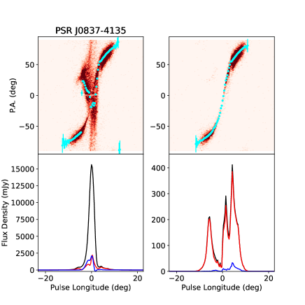
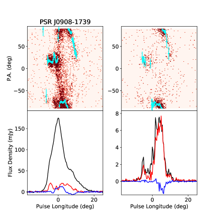
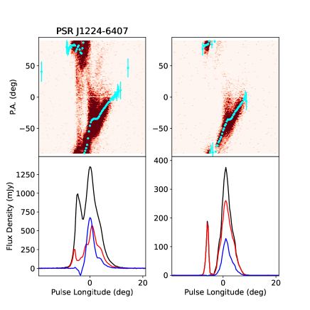
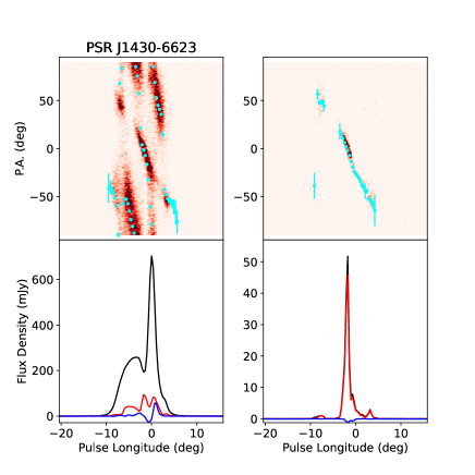
Figure 1: Results for four pulsars with non-RVM PPA tracks after integrating all the single pulses. Each pulsar’s data is represented by four panels. The top left panel shows in cyan the position angle of the linear polarization in the integrated profile superposed on a heat-map of all the individual position angle points. The bottom left panel show the integrated profile (black), the linear polarization (red) and the circular polarization (blue). The right hand panels depict the same scheme but only for those samples which are more than 80% polarized.

Instead of integrating over many rotations of the pulsar, examination of the polarization on a continuous train of time-samples (typically of duration 1 ms or less) often provides a better understanding of the PPA behaviour. Gil & Lyne (1995) showed that in a pulsar with a complex non-RVM like PPA traverse, the time-sampled PPA distribution clearly showed two parallel orthogonal RVM tracks. However the many PPA values which did not conform to the RVM were then speculated to be due to mode mixing and propagation effects. This aspect of OPM averaging has also been seen in other studies of bright pulsars (e.g. Rankin & Rathnasree 1995; Ramachandran et al. 2004; Mitra et al. 2016a). A handful of these time-sampled polarization emission surveys have been carried out for normal pulsars (Manchester et al. 1975; Stinebring et al. 1984; Mitra & Rankin 2011; Mitra et al. 2016b; Olszanski et al. 2019), where often RVM-like OPM tracks are seen in many pulsars across different frequencies. These OPM tracks are usually thought to be associated with the natural modes i.e. the extraordinary (X) and ordinary (O) propagation modes of pair plasma embedded in the strong magnetic field (Cocke & Pacholczyk, 1976; Melrose & Stoneham, 1977) .

There exists another category of pulsars which are significant in number, where the time-sampled PPA appear to show no organized pattern and the corresponding average PPA has a complex non-RVM like behaviour. Recently Mitra et al. (2023a) (MMB23 hereafter) claimed that the high linearly polarized time samples must correspond to purely linearly polarized X and O mode of the strongly magnetized pair plasma, and if the underlying emission mechanism is excited due to coherent curvature radiation (CCR hereafter), then these time samples across the pulse should reproduce the RVM. This line of reasoning is similar to an earlier study by Mitra et al. (2009) and Melikidze et al. (2014) where they demonstrated that the PPA corresponding to the high linearly polarized subpulses in several pulsars follow the average RVM like PPA traverse. MMB23 applied the high linearly polarized time sample criterion to PSR J1645$-$0317, which has a disordered single pulse PPA distribution and complex non-RVM average PPA traverse. Remarkably they found that the high linearly polarized samples followed the PPA track which can be fitted with the RVM accurately. In this case only one PPA track was clearly visible, and a hint of presence of high linearly polarized orthogonal PPAs for a small range of pulse longitude was seen. MMB23 surmised that the low linearly polarized samples dominate the disordered non-RVM PPAs, presumably due to mixing of the modes and propagation effects.

The high linearly polarized sample criteria can hence be employed to a larger dataset to check two predictions of MMB23: firstly in pulsars with disordered PPA the high linearly polarized samples should follow the RVM and secondly there must be several cases where these samples follow the two tracks of X and O mode. The sample set used by J23 is particularly suitable for this exercise, since for many pulsars high quality, high time-resolution data have also been recorded. In this paper we report an analysis of high linearly polarized samples from the TPA observations. In section 2 we define the sample selection, section 3 we describe the analysis technique and present the results and in section 4 we state our conclusions.

2 Sample selection

The Thousand Pulsar Array Program (TPA) on MeerKAT has observed in excess of 1200 pulsars (Johnston et al., 2020). The integration time on each of the pulsars was generally sufficient to produce at least 1000 single pulses (Song et al., 2021). Details of the TPA observing, processing, calibration and analysis can be found in Serylak et al. (2021), Posselt et al. (2021) and Song et al. (2023). In brief the observing band runs from 896 to 1671 MHz subdivided into 1 MHz channels. Typically 1024 phase bins per pulsar period are formed and the data are both flux and polarization calibrated.

In this paper we used high time-resolution data for 1202 pulsars. From the J23 paper, these pulars are classified as follows: 411 follow the RVM, 342 are non-RVM, 70 are ‘flat’ i.e no significant PPA changes across the pulse profile but still can be fitted with RVM, 20 are interpulses and for 359 no RVM fit was attempted. In J23, the signal-to-noise ratio (s/n) of the linear polarization in the integrated profile was critical, here however, we require good s/n for each single pulse and we need sufficient single pulses to build up the statistics. We therefore restricted the sample to (a) pulsars with more than 500 pulses and (b) at least 60% of the single pulses had to have s/n more than 5-$\sigma$ in Stokes $I$. This resulted in a sample of 249 pulsars.

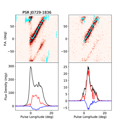
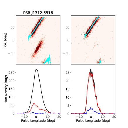
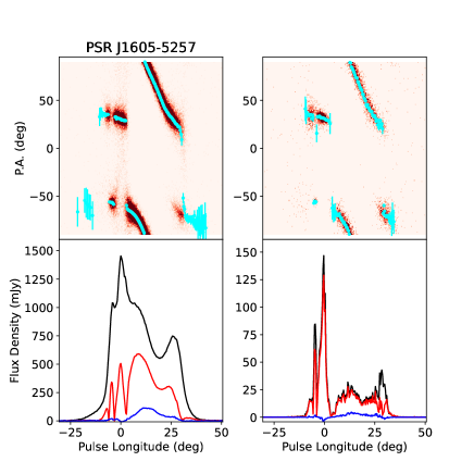
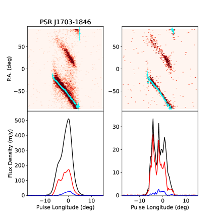
Figure 2: Results for four pulsars showing RVM tracks with orthogonal jumps. Each pulsar’s data is represented by four panels. The top left panel shows in cyan the position angle of the linear polarization in the integrated profile superposed on a heat-map of all the individual position angle points. The bottom left panel show the integrated profile (black), the linear polarization (red) and the circular polarization (blue). The right hand panels depict the same scheme but only for those samples which are more than 80% polarized.

3 Results and Analysis

3.1 Forming the highly polarized profiles

The analysis proceeded as follows. First we summed together all the data modulo the pulsar spin period to produce the average pulse profile and set the on-pulse window. At the same time, for each phase bin within the pulse window we computed the PPA provided the linear polarization was more than 3.5-$\sigma$ above the noise. Then we made a second pass through the high time-resolution data, this time only recording samples which are greater than 80% linearly polarized. We kept track of the number of occurrences of such samples as a function of pulse longitude. As before, we computed the PPA for each of these samples. Finally, we produce an integrated profile from these high polarized samples and an integrated PPA swing. We stress that we deal with individual time samples, we do not consider single pulses as a whole nor any specific sub-structure within the single pulse profile.

In Figure 1 we show the output from four pulsars, all of which were classified as non-RVM in J23. The most noticeable aspect here is that on application of the high polarized time sample criterion, the disordered PPA distribution (seen in the left top heat map) vanishes, and a more ordered narrowly confined PPA distribution is observed (seen in the right top heat map). Consequently the distortions in the average PPA tracks (cyan points in the left top panel) smooth out, and more RVM-like tracks appear (cyan points in the right top panel). The effect is striking in PSR J0837$-$4135, where the classical RVM-like PPA becomes apparent. In PSR J0908–1739, the OPM in the leading part of the profile gets clearly resolved. In PSR J1224–6407, while most of the disordered PPA distribution vanishes leaving behind a narrowly defined PPA track, one can still see some excess spread of PPA towards the center of the profile which results in a small kinky feature in average PPA. In PSR J1430–6623 the several PPA patches almost disappear in the high polarized case and only a single RVM like PPA track is seen.

In Figure 2 we show four examples of pulsars that were classified as RVM in J23. After applying the high polarized criteria the average PPA traverse for these pulsars still follows the RVM. The high polarized PPA distributions show assorted properties: in PSRs J0729–1836 and J1703–1846 the two parallel OPM tracks are seen in both the full and high polarized case; in PSR J1312–5516 two tracks are seen in the full data while only one track is visible in high polarized case; in PSR J1605–5257 the multiple OPM jumps in the full data are reproduced in the high polarized data.

It should be noted that, for low $\dot{E}$ pulsars, only a few percent of the samples go into making the profiles shown in Figures 1 and 2. This would imply that part of the depolarization is due to the spread of the PPA, but most of the depolarization must already occur internally in the magnetosphere, before the emission detaches.

Table 1: Results for the 249 pulsars analysed here. The first column is the classifcation given by the RVM fitter (see J23 for details). The second and third column denote how many pulsars fall into each class according to J23 and from the present work.

Class	J23	current work
RVM	90	146
Flat	11	9
non-RVM	146	22
No Pol	2	72

3.2 RVM fitting

The same RVM fitter that was used in J23 was now used to fit the high linearly polarized average PPA tracks for all 249 pulsars with the results given in Table 1. None of the pulsars previously classified as RVM became non-RVM after selecting the high polarized samples. In 72 of the 249 pulsars, there were not sufficient PPA points for the fitter to proceed (i.e. there were not sufficient highly polarized samples). Of the 177 remaining pulsars we found that only 22, i.e. 12%, failed to give good fits with $\chi^{2}$ values less than 3 and hence were classified as non-RVM. This is a significant improvement over the results of J23, where RVM failed to fit to the average PPA for 59% of the pulsars under consideration here.

We carefully scrutinized the 22 cases which the fitter classified as ‘non-RVM’. These cases may be influenced by our analysis method, where due to practical considerations for retaining sufficient time samples we have defined the high linearly polarized sample to be above 80%, whereas MMB23 suggest that the RVM will be reproduced only by 100% linearly polarized samples. The lower fractional polarization can be a result of mixing of the X and O modes, and it is possible that this leads to deviation from the RVM. We tested this by re-analysing the data for these 22 pulsars when setting the threshold to 90% linear rather than 80%. This indeed reduces the number of non-RVM cases to 9. We surmise that more sensitive observations and a larger number of pulsar rotations would be beneficial to sort out the remaining cases.

In Figure 3 we show the cumulative $\dot{E}$ distributions for the entire TPA sample of 1202 pulsars, the 249 pulsars considered here and the 72 pulsars without any highly polarized samples. Two points can be gleaned. First the 249 pulsars are somewhat lower in $\dot{E}$ than the entire sample; this implies that single pulses from lower $\dot{E}$ pulsars are brighter than those from high $\dot{E}$ pulsars (possibly due to the fact that their distances are smaller). Secondly the pulsars without highly polarized data points are significantly lower in $\dot{E}$ than the sample as a whole. However, we caution that with only $\sim$1000 single pulses per pulsar that some of the seemingly unpolarized cases may be resolved with a much larger number of pulses. This will not be true in all cases, for example the very bright PSR J1534–5334 shows no samples with linear polarization greater than 50%.

3.3 Circular Polarization and OPM jumps

In the profiles made from the highly linearly polarized samples there often remains a significant degree of circular polarization, for example PSR J1224–6407 in Figure 1 and PSRs J0729–1836 and J1312–5516 in Figure 2. One possibility is that the modes are elliptically polarized. For PSR J1312–5516 in particular the standard integrated profile with its two competing modes shows almost no circular whereas in the highly polarized profile a single mode dominates with positive circular polarization.

In the highly polarized profiles we find that OPM tracks are present in 35% of cases, a number not too dissimilar to that found by J23 in a much larger sample of integrated pulse profiles. For the pulsars which do show evidence of OPM jumps in J23, 50% of them retain the OPM jumps in the highly polarized profiles. It therefore seems clear that sometimes the X mode provides the highly polarized samples, sometimes in the O mode and sometimes a mixture of the two as a function of pulse longitude. In regions of pulse longitude where there are mode mixtures, we find that the average PPA tends to follow one of the modes, and the OPM jumps in the average PPA can be clearly distinguished. The RVM fitter is designed to detect OPM jumps of 90°, and hence fitting RVM to the average PPA performs well. For a given pulsar there is no immediate way to tell which of O or X is the dominant mode. Thus, any theoretical emission model should take this into account.

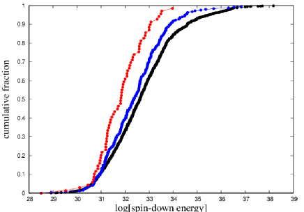
Figure 3: Cumulative distributions of the log of the spin-down energy, $\dot{E}$, for the 1202 pulsars from the TPA (black), the 249 pulsars used in this sample (blue) and the 69 pulsars with no highly polarized samples (red).

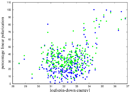
Figure 4: Percentage linear polarization as a function of $\dot{E}$. The blue points show the linear polarization of the integrated profile, the green points show the mean linear polarization of the individual samples..

3.4 Tabular description of results

In Table 2 we present the results for the 249 pulsars analysed here using the selection criteria outlined in Section 2. The first two columns report the pulsar’s Jname and the log of the spin-down energy ($\dot{E}$). Columns 3 and 4 given the number of single pulses recorded ($N_{p}$) and the percentage of those above 5-$\sigma$ ($N_{f}$). Columns 5 and 6 give the percentage of linear ($\%L_{t}$) and circular ($\%V_{t}$) polarization in the integrated profile. Note that these values may differ slightly from those given in Posselt et al. (2023) as the observations used here are not necessarily the same as used in their paper. Columns 7 and 8 give the mean percentage of all the samples in linear ($\%L_{s}$) and circular ($\%V_{s}$) polarization provided that the total intensity of the sample is greater than 3.5-$\sigma$. The last two columns give the class from the RVM fitting according to J23 and after formation of the high linear profile. We denote with a dagger symbol those pulsars which remain non-RVM even after the application of a higher linear threshold as outlined in Section 3.2.

Figure 4 shows the percentage linear polarization of the integrated profile (blue points) and the average of the individual samples (green points). First it should be noted the relative paucity of points above an $\dot{E}$ of $10^{34}$ ergs^-1. This is because these pulsars are generally too weak to satisfy our single pulse thresholds. However, the blue points show the trend pointed out by Weltevrede & Johnston (2008), Posselt et al. (2023) and others in that pulsars with high $\dot{E}$ are highly polarized whereas pulsars at low $\dot{E}$ much less so. In the single samples we see, as expected, that the fractional linear polarization increases. The trend still remains; relatively few pulsars at low $\dot{E}$ have a fractional polarization greater than 50%. This implies that the majority of samples must have fractional linear polarization less than 25% and that the modes have already mixed on this short time-scale.

4 Conclusions

MMB23 suggest that if the underlying emission mechanism is CCR, then high linearly polarized samples in pulsars should have orthogonal PPA tracks that follow the RVM. We tested this hypothesis on the sample set of TPA pulsars. We found that in pulsars with a disordered PPA distribution, the RVM can be recovered in the vast majority of cases. Further, we clearly see examples of high linearly polarized OPM tracks which can be interpreted as the X and O modes of the strongly magnetized pair plasma. The escape of the X and O modes requires the plasma flow to be inhomogeneous and Mitra et al. (2023b) alluded to the fact that the observed change in degree of linear polarization with pulsar spindown energy may be related to the change in the degree of inhomogeneity in the plasma.

Mitra et al. (2023b) suggested that as the linearly polarized modes propagate through the magnetospheric plasma, the modes can get partially converted into circular polarization due to propagation effects, and thus the observed signals are generally elliptically polarized. The non-RVM PPAs can be interpreted as incoherent averaging of the X and O mode from a large number of sources. A different idea was put forward by Oswald et al. (2023b). In their picture, both coherent and incoherent mixing of the modes take place, the coherent mixing produces the circular polarization and also distorts the PPA. This model provides a good fit to the broad-band data presented in Oswald et al. (2023a).

CCR can be excited in a pulsar plasma by a stable charge bunch streaming at relativistic speeds along the curved magnetic field. Theoretically, formation of relativistic charge solitons is thought to be an excellent candidate for the formation of such charge bunches (Melikidze & Pataraia 1980; Asseo & Melikidze 1998; Melikidze et al. 2000; Lakoba et al. 2018; Rahaman et al. 2020; Manthei et al. 2021; Rahaman et al. 2022b). The theory of charge solitons has been developed in the one dimensional approximation, and further improvement in the theory in needed to verify the stability of the solitons in a more realistic situation of two or three dimension. Further the physical process of the escape of X and O mode in pulsar plasma and the origin of circular polarization still needs to be understood (e.g. Melikidze et al. 2014; Rahaman et al. 2022a; Mitra et al. 2023b). The observational evidence for CCR presented in this work strongly motivates theoretical research in these directions.

Data Availability

Data are available on reasonable request.

Appendix A Table of Results

Table 2 lists the 249 pulsars used in this analysis. For a description of the table see Section 3.4.

Table 2: Results for 249 pulsars. The first two columns report the pulsar’s Jname and the log of the spin–down energy ($\dot{E}$). Columns 3 and 4 given the number of single pulses recorded ($N_{p}$) and the percentage of those above 5–$\sigma$ ($N_{f}$). Columns 5 and 6 give the percentage of linear ($\%L_{t}$) and circular ($\%V_{t}$) polarization in the integrated profile. Columns 7 and 8 give the mean percentage of all the samples in linear ($\%L_{s}$) and circular ($\%V_{s}$) polarization. The last two columns give the Class from the RVM fitting according to Johnston et al. (2023) and after formation of the high linear profile. The dagger symbol denotes pulsars which remain non–RVM even after application of a higher linear threshold.

JNAME	log($\dot{E}$)	$N_{p}$	$N_{f}$	$\%L_{t}$	$\%V_{t}$	$\%L_{s}$	$\%V_{s}$	Old Class	New Class
J0034–0721	31.3	1042	54.5	15.9	4.4	37.4	4.0	non–RVM	RVM
J0108–1431	30.8	1042	55.6	80.6	12.1	69.5	7.4	flat	flat
J0134–2937	33.1	1110	88.1	51.4	–20.3	47.9	–13.7	RVM	RVM
J0151–0635	30.7	1039	97.6	38.9	0.2	41.0	–1.0	RVM	RVM
J0152–1637	31.9	1047	86.4	15.7	–1.4	25.8	–1.6	non–RVM	No poln
J0255–5304	31.1	1226	81.9	9.2	–5.0	31.3	–4.5	non–RVM	non–RVM
J0302+2252	30.3	1030	57.2	25.4	–0.2	40.9	–0.1	non–RVM	non–RVM
J0304+1932	31.3	1032	89.2	36.8	12.5	45.0	12.6	RVM	RVM
J0401–7608	32.6	1078	98.1	28.8	–2.3	34.8	–2.4	non–RVM	RVM
J0448–2749	31.8	1048	58.1	23.1	–15.3	36.1	–17.3	flat	flat
J0452–1759	33.1	1042	100.0	18.3	–0.0	33.7	0.5	RVM	RVM
J0517+2212	31.6	1036	83.0	21.1	6.1	30.2	6.7	non–RVM	RVM
J0525+1115	31.8	1048	95.1	13.8	9.1	24.5	9.2	non–RVM	No poln
J0536–7543	31.1	1041	92.6	51.5	–11.6	55.3	–10.9	RVM	RVM
J0543+2329	34.6	1033	97.8	53.3	–11.1	61.7	–12.2	RVM	RVM
J0601–0527	32.9	1063	96.9	32.1	1.5	38.4	–0.5	non–RVM	RVM
J0614+2229	34.8	1032	100.0	76.9	16.2	80.5	15.9	RVM	RVM
J0624–0424	31.5	1056	97.5	28.8	6.3	41.5	6.1	non–RVM	non–RVM
J0629+2415	32.9	1030	100.0	23.5	11.1	31.7	11.7	non–RVM	RVM
J0630–2834	32.2	1043	100.0	52.1	–5.1	55.1	–4.9	RVM	RVM
J0646+0905	31.6	1046	87.4	37.5	–3.8	40.7	–3.8	RVM	RVM
J0659+1414	34.6	1047	63.4	85.8	–14.0	88.4	–14.4	RVM	RVM
J0719–2545	32.5	1043	48.1	21.6	8.3	28.7	8.3	non–RVM	RVM
J0729–1836	33.7	1042	80.7	27.2	–8.3	40.1	–8.2	RVM	RVM
J0738–4042	33.0	1095	100.0	27.1	–6.2	43.7	–6.0	non–RVM	RVM
J0742–2822	35.1	2969	100.0	90.4	–4.8	93.0	–4.9	RVM	RVM
J0758–1528	32.3	1044	79.3	18.8	–1.1	32.0	–0.8	non–RVM	RVM
J0809–4753	32.9	1044	99.8	27.4	–0.9	31.2	–0.8	non–RVM	RVM
J0818–3232	30.5	1029	79.6	20.2	–3.8	33.1	–2.9	non–RVM	No poln
J0820–1350	31.6	1056	98.0	14.6	–9.7	27.4	–10.3	non–RVM	RVM
J0820–4114	30.7	1048	93.9	30.6	3.3	31.4	2.2	No poln	RVM
J0823+0159	30.8	1076	99.3	10.9	–2.3	31.4	–1.8	non–RVM	RVM
J0835–4510	36.8	3433	100.0	88.0	–9.0	88.9	–9.3	RVM	RVM
J0837+0610	32.1	1037	92.4	8.6	–4.4	28.5	–4.2	non–RVM	No poln
J0837–4135	32.5	1041	99.5	15.8	12.4	30.1	12.5	non–RVM	RVM
J0840–5332	32.2	1035	97.0	17.6	14.1	27.0	14.5	non–RVM	RVM
J0846–3533	31.7	1033	99.9	40.3	–10.4	42.0	–10.8	non–RVM	RVM
J0855–3331	32.1	1030	64.2	15.5	2.2	28.3	2.4	non–RVM	No poln
J0856–6137	31.9	1033	86.6	3.7	5.0	10.9	4.8	RVM	No poln
J0902–6325	31.2	1033	97.6	33.9	6.9	38.5	8.9	non–RVM	RVM
J0904–7459	32.0	1040	86.0	32.6	2.1	33.6	1.5	RVM	RVM
J0905–4536	30.8	1030	89.3	41.4	2.5	45.5	1.4	RVM	RVM
J0905–5127	34.4	1064	2.4	100.2	8.2	84.2	9.4	RVM	RVM
J0907–5157	33.6	1073	100.0	37.1	3.1	44.0	2.3	RVM	RVM
J0908–1739	32.6	1050	61.9	13.8	1.9	30.2	2.9	non–RVM	RVM
J0908–4913	35.7	1045	100.0	98.1	1.1	96.1	1.0	RVM	RVM
J0909–7212	30.7	1035	70.8	32.4	9.2	38.7	8.0	RVM	RVM
J0922+0638	33.8	2090	100.0	55.2	8.6	58.5	8.5	RVM	RVM
J0924–5302	33.5	1032	92.8	8.5	–5.9	13.3	–6.3	non–RVM	No poln
J0924–5814	32.7	1044	99.9	53.9	–3.9	56.1	–4.2	RVM	RVM
J0934–5249	31.8	1031	98.5	19.4	–12.8	35.0	–12.4	non–RVM	RVM
J0942–5552	33.5	1040	98.1	38.9	–2.6	48.1	0.8	non–RVM	RVM
J0944–1354	31.0	1041	98.7	20.1	16.0	29.4	15.4	non–RVM	No poln
J0953+0755	32.7	803	99.8	14.0	–5.6	37.0	–6.5	non–RVM	RVM

Table 2: Results for 249 pulsars (continued)

JNAME	log($\dot{E}$)	$N_{p}$	$N_{f}$	$\%L_{t}$	$\%V_{t}$	$\%L_{s}$	$\%V_{s}$	Old Class	New Class
J0959–4809	31.0	1049	95.3	43.9	–7.8	39.6	–10.6	RVM	RVM
J1001–5507	32.8	1030	100.0	6.7	–0.6	15.4	–0.9	non–RVM	No poln
J1001–5559	30.9	1031	88.8	23.2	10.2	30.5	13.1	non–RVM	No poln
J1001–5939	30.7	517	43.3	35.3	1.2	39.1	0.8	RVM	No poln
J1016–5345	32.2	1033	51.8	20.4	3.7	30.1	3.8	RVM	RVM
J1017–5621	33.0	1046	73.3	18.4	–17.1	48.1	–17.4	non–RVM	non–RVM$\dagger$
J1018–1642	31.1	1029	61.7	16.7	20.3	34.9	24.0	non–RVM	non–RVM
J1034–3224	30.8	1035	100.0	8.2	5.8	13.2	4.5	non–RVM	No poln
J1041–1942	31.1	1055	98.3	33.4	7.6	43.0	8.8	RVM	RVM
J1042–5521	32.2	1032	86.1	11.9	3.9	20.1	–6.3	RVM	No poln
J1048–5832	36.3	7270	85.3	72.2	4.5	74.0	4.8	RVM	RVM
J1049–5833	31.2	1035	48.9	25.6	–7.6	38.6	–7.7	RVM	No poln
J1056–6258	33.3	1049	100.0	44.4	–2.4	51.7	–2.5	flat	flat
J1057–5226	34.5	1022	100.0	69.1	0.1	75.5	–0.2	non–RVM	non–RVM$\dagger$
J1059–5742	32.0	1054	96.3	10.0	–0.4	22.6	0.1	non–RVM	No poln
J1110–5637	32.7	1041	95.8	28.7	–8.0	36.7	–8.9	RVM	RVM
J1112–6613	32.9	1033	99.9	17.6	7.2	18.5	8.0	non–RVM	RVM
J1112–6926	32.3	1036	63.0	11.0	3.1	21.3	2.9	non–RVM	No poln
J1114–6100	33.4	1036	83.9	18.9	–0.8	27.3	–1.5	RVM	RVM
J1116–4122	32.6	1037	82.7	10.0	–0.8	28.8	–1.4	RVM	No poln
J1121–5444	32.9	1033	99.3	26.7	–7.3	27.7	–7.7	non–RVM	RVM
J1123–4844	32.3	1057	96.7	31.7	27.0	34.0	26.3	non–RVM	RVM
J1133–6250	31.2	1033	92.2	13.9	2.5	23.3	1.6	non–RVM	No poln
J1136+1551	31.9	1031	85.0	18.5	–8.1	34.6	–8.4	non–RVM	RVM
J1136–5525	33.8	1047	98.6	9.3	–2.2	25.0	–1.9	non–RVM	RVM
J1137–6700	31.2	1096	93.6	14.6	–1.9	23.3	–0.9	flat	No poln
J1141–6545	33.4	5200	85.4	13.6	5.7	19.7	4.5	RVM	RVM
J1146–6030	33.5	1067	97.5	26.9	3.3	41.2	4.2	RVM	RVM
J1157–6224	33.4	1052	97.6	32.6	10.8	38.1	8.9	non–RVM	non–RVM
J1202–5820	33.0	1031	98.7	28.0	7.8	45.2	7.0	non–RVM	RVM
J1224–6407	34.3	1071	100.0	35.4	22.5	50.5	22.9	non–RVM	RVM
J1232–4742	28.9	962	82.1	33.2	–2.9	38.1	–4.1	flat	flat
J1237–6725	31.0	1030	58.5	2.5	1.2	9.4	1.0	non–RVM	No poln
J1239+2453	31.1	1029	94.8	42.1	0.4	47.9	0.2	non–RVM	RVM
J1243–6423	33.5	1058	99.6	24.6	–3.5	31.4	–2.8	non–RVM	non–RVM
J1246+2253	31.5	1032	50.9	8.8	–2.1	29.3	–3.4	non–RVM	No poln
J1253–5820	33.7	1068	98.8	63.2	6.8	73.1	7.0	RVM	RVM
J1257–1027	31.8	1072	97.2	33.4	–4.8	37.5	–3.5	non–RVM	non–RVM
J1305–6455	32.9	1036	98.8	35.2	10.4	31.0	13.1	non–RVM	non–RVM
J1306–6617	33.3	1037	95.6	17.3	7.5	24.9	7.6	non–RVM	No poln
J1312–5516	32.6	709	94.6	21.9	0.1	39.2	–0.5	RVM	RVM
J1320–5359	34.2	1043	86.9	26.0	–8.9	31.9	–7.2	RVM	RVM
J1326–5859	33.1	1048	96.5	37.5	8.6	39.0	8.7	non–RVM	RVM
J1326–6408	32.4	1034	85.6	24.5	2.5	25.1	1.9	non–RVM	No poln
J1326–6700	33.1	1037	99.8	36.8	–5.8	52.6	–6.1	RVM	RVM
J1327–6222	33.7	1043	100.0	6.4	5.0	16.5	4.0	non–RVM	RVM
J1327–6301	33.9	1075	96.4	29.7	0.2	31.7	2.0	RVM	RVM
J1328–4357	32.9	1038	89.1	32.5	6.4	42.2	6.9	RVM	RVM
J1328–4921	30.9	527	85.2	17.6	6.7	24.2	3.1	non–RVM	No poln
J1338–6204	32.5	1034	99.8	21.4	13.3	24.9	14.2	non–RVM	RVM
J1355–5153	32.6	933	86.2	2.4	–2.1	7.0	–2.9	non–RVM	No poln
J1401–6357	33.0	1035	97.6	26.7	–0.9	40.2	0.1	RVM	RVM
J1414–6802	30.4	538	68.8	34.0	11.3	42.7	11.7	RVM	RVM
J1420–5416	31.0	1025	52.2	11.5	–13.9	18.8	–14.4	non–RVM	No poln
J1424–5822	33.5	1028	49.1	21.8	3.2	18.7	4.1	flat	No poln

Table 2: Results for 249 pulsars (continued)

JNAME	log($\dot{E}$)	$N_{p}$	$N_{f}$	$\%L_{t}$	$\%V_{t}$	$\%L_{s}$	$\%V_{s}$	Old Class	New Class
J1428–5530	32.6	1037	72.1	30.9	0.7	42.4	0.8	RVM	RVM
J1430–6623	32.4	1040	100.0	15.2	2.1	29.1	1.6	non–RVM	RVM
J1440–6344	32.7	1032	85.8	21.3	3.2	27.5	5.0	non–RVM	No poln
J1453–6413	34.3	1087	92.7	31.4	4.4	35.6	4.9	non–RVM	RVM
J1456–6843	32.3	1075	99.8	9.8	1.5	38.7	–1.0	non–RVM	non–RVM
J1507–4352	33.4	1043	91.7	27.9	–6.2	34.5	–6.5	RVM	RVM
J1507–6640	33.0	1042	50.8	8.9	7.4	21.1	6.4	non–RVM	No poln
J1514–4834	32.6	1043	48.5	7.5	–3.4	19.8	–1.8	non–RVM	No poln
J1522–5829	33.1	1046	98.1	28.7	1.4	32.5	1.5	non–RVM	RVM
J1527–3931	31.7	743	50.3	16.3	12.7	23.7	11.5	RVM	No poln
J1527–5552	32.6	1030	55.2	18.4	13.9	20.6	13.4	non–RVM	No poln
J1534–5334	31.3	1032	100.0	4.2	0.9	10.8	0.0	non–RVM	No poln
J1535–4114	33.3	1043	62.1	51.8	–11.2	22.6	–62.6	RVM	RVM
J1536–3602	31.1	1032	61.4	25.8	–7.6	37.5	–9.3	non–RVM	RVM
J1539–5626	34.1	1078	89.4	32.7	1.6	27.9	–0.9	non–RVM	RVM
J1539–6322	30.3	1104	91.1	48.8	5.4	49.2	5.9	RVM	RVM
J1543+0929	31.6	1028	98.9	26.5	–4.9	30.2	–9.4	non–RVM	RVM
J1544–5308	32.6	1087	99.8	17.8	–4.1	25.4	–5.5	non–RVM	RVM
J1555–2341	32.3	1046	83.9	19.3	2.0	35.2	2.3	RVM	RVM
J1555–3134	31.3	1045	99.8	16.0	2.9	26.9	2.7	non–RVM	No poln
J1557–4258	32.6	1038	85.7	32.2	–13.8	39.1	–15.3	non–RVM	non–RVM
J1559–4438	33.4	1066	100.0	41.0	–10.3	42.0	–10.0	RVM	RVM
J1602–5100	33.6	1030	94.3	20.6	6.0	28.6	–4.4	non–RVM	RVM
J1603–2531	33.4	2131	94.3	27.7	0.6	44.5	–0.4	flat	flat
J1603–2712	32.4	1030	64.8	33.1	1.2	40.0	1.7	non–RVM	non–RVM
J1604–4909	33.0	1043	99.9	9.8	0.8	17.1	1.1	non–RVM	No poln
J1604–7203	31.9	1764	93.0	20.2	5.5	23.6	4.9	non–RVM	No poln
J1605–5257	31.5	1037	99.8	37.0	5.1	45.0	4.9	RVM	RVM
J1607–0032	32.2	1031	95.3	7.2	1.6	29.9	–0.2	non–RVM	No poln
J1622–4332	31.9	1039	58.5	16.8	12.4	25.2	8.8	non–RVM	No poln
J1623–0908	31.7	1030	52.3	2.0	2.8	7.8	1.9	non–RVM	No poln
J1625–4048	30.1	523	44.0	19.7	1.6	22.3	2.0	non–RVM	No poln
J1635–5954	32.6	1030	97.9	36.8	8.1	34.9	8.8	non–RVM	RVM
J1645–0317	33.1	1062	100.0	12.8	–1.2	24.2	–0.7	non–RVM	RVM
J1646–6831	31.1	1031	70.2	40.6	6.8	46.8	6.2	non–RVM	non–RVM$\dagger$
J1650–1654	31.4	1029	66.0	19.7	7.2	36.6	4.8	non–RVM	No poln
J1651–4246	32.5	2143	96.1	39.6	–15.4	43.5	–13.7	non–RVM	RVM
J1651–5222	32.4	1054	99.2	19.9	–5.6	34.9	–5.3	non–RVM	RVM
J1700–3312	31.9	1037	76.0	38.4	–15.2	44.0	–14.8	RVM	RVM
J1703–1846	32.1	1057	67.8	34.5	3.9	48.0	4.2	RVM	RVM
J1703–3241	31.2	1040	99.7	46.2	–0.5	52.5	–0.6	RVM	RVM
J1705–1906	33.8	868	100.0	53.2	–17.5	58.1	–17.6	non–RVM	non–RVM$\dagger$
J1705–3423	33.4	1098	97.4	13.7	1.9	19.4	2.3	non–RVM	RVM
J1709–1640	32.9	1033	96.0	10.5	2.0	31.9	2.4	RVM	RVM
J1709–4429	36.5	2204	93.0	97.5	–21.3	86.9	–21.3	flat	flat
J1711–5350	32.9	669	60.5	11.9	–2.3	22.5	–0.5	non–RVM	RVM
J1720–1633	31.8	1033	76.8	17.3	3.5	24.1	2.1	RVM	RVM
J1720–2933	32.1	1048	69.8	15.6	5.7	29.8	5.2	RVM	No poln
J1722–3207	32.4	1068	100.0	23.9	1.1	26.6	0.7	RVM	RVM
J1722–3712	34.5	1100	34.5	54.8	12.4	41.3	12.2	RVM	RVM
J1731–4744	34.0	1049	100.0	18.0	4.0	37.8	3.7	non–RVM	non–RVM$\dagger$
J1735–0724	32.8	1072	91.0	28.5	0.9	33.9	1.9	non–RVM	RVM
J1738–3211	31.8	1054	52.4	17.9	–5.0	44.0	–5.5	non–RVM	non–RVM$\dagger$
J1740+1000	35.4	1311	77.0	99.7	–3.1	84.6	–2.2	RVM	RVM
J1740+1311	32.0	1039	98.9	44.5	4.1	49.7	4.0	RVM	RVM

Table 2: Results for 249 pulsars (continued)

JNAME	log($\dot{E}$)	$N_{p}$	$N_{f}$	$\%L_{t}$	$\%V_{t}$	$\%L_{s}$	$\%V_{s}$	Old Class	New Class
J1740–3015	34.9	1032	99.7	85.3	–34.0	85.3	–34.9	RVM	RVM
J1741–0840	31.0	1037	71.8	37.4	–4.4	44.0	–4.1	RVM	RVM
J1741–3927	32.7	1055	100.0	25.2	4.5	29.9	4.7	non–RVM	RVM
J1742–4616	31.3	1035	38.5	36.9	–8.9	39.6	–8.9	flat	No poln
J1743–3150	32.5	1035	89.1	23.4	–3.7	27.8	–3.0	RVM	RVM
J1744–1610	31.2	569	62.4	21.0	–2.6	27.2	–2.4	non–RVM	No poln
J1745–3040	33.9	1060	78.5	49.5	–2.7	53.6	–3.5	non–RVM	non–RVM
J1748–1300	32.9	1041	93.8	26.9	3.5	30.3	4.5	RVM	RVM
J1750–3157	31.0	1043	59.4	11.1	–2.7	17.3	–3.3	non–RVM	No poln
J1751–4657	32.1	1050	97.0	17.9	9.1	30.5	8.7	non–RVM	RVM
J1752–2806	33.3	1050	99.9	11.1	2.8	36.6	4.6	non–RVM	non–RVM$\dagger$
J1759–3107	32.1	1032	45.8	24.2	1.0	33.2	–3.6	RVM	RVM
J1801–2920	32.0	1029	78.3	44.7	–6.9	48.5	–6.6	RVM	RVM
J1806–1154	32.6	1030	94.3	35.6	–0.3	35.8	–0.8	RVM	RVM
J1807–0847	32.4	1123	99.9	24.6	5.6	31.3	6.0	non–RVM	RVM
J1808–0813	31.9	1034	80.2	23.1	6.8	31.4	7.0	RVM	RVM
J1810–5338	32.9	2300	99.9	43.5	–0.3	42.0	–1.4	RVM	RVM
J1817–3618	33.1	1063	68.8	19.4	–12.4	32.5	–13.2	RVM	RVM
J1817–3837	32.6	1068	96.8	14.9	0.7	31.8	1.1	non–RVM	RVM
J1819+1305	31.1	1034	60.2	21.2	–1.9	28.1	–2.8	RVM	RVM
J1820–0427	33.1	1138	94.1	22.9	–6.2	30.2	–6.1	non–RVM	RVM
J1823+0550	31.3	1032	100.0	22.4	3.9	31.5	3.8	non–RVM	RVM
J1823–3106	33.7	1201	91.6	44.4	–4.9	47.0	–4.6	RVM	RVM
J1824–1945	34.5	1112	97.7	18.9	–2.3	20.9	–2.6	non–RVM	RVM
J1825–0935	33.7	1031	99.9	34.5	4.4	38.2	3.7	non–RVM	non–RVM$\dagger$
J1826–1131	31.3	1032	87.0	0.8	–6.3	9.1	–4.2	non–RVM	No poln
J1829–1751	33.9	685	100.0	35.5	–9.3	39.7	–9.6	non–RVM	flat
J1832–0827	34.0	1052	81.3	14.8	–2.3	24.1	–0.9	non–RVM	No poln
J1834–0426	32.1	1071	100.0	28.2	–1.8	23.9	–2.3	No poln	RVM
J1836–1008	33.4	1041	100.0	14.7	5.2	18.3	5.2	non–RVM	No poln
J1837–0653	30.6	1029	54.4	20.2	–4.2	28.3	–7.5	non–RVM	No poln
J1839–1238	31.4	1034	66.7	21.1	7.2	23.8	6.9	RVM	No poln
J1840–0809	32.0	1030	86.3	32.6	–10.7	36.1	–9.7	RVM	RVM
J1840–0815	31.9	1029	78.0	7.3	–0.9	15.8	–0.1	non–RVM	No poln
J1842–0359	30.5	1035	98.9	52.1	3.7	51.2	3.3	RVM	RVM
J1843–0000	32.7	1028	100.0	15.5	–0.6	35.8	–0.8	RVM	RVM
J1844+1454	33.1	1030	96.0	36.1	0.5	36.7	0.5	non–RVM	RVM
J1847–0402	34.0	1054	99.7	17.1	2.2	24.3	2.3	non–RVM	RVM
J1848–0123	32.9	1047	100.0	4.8	0.9	7.8	1.0	non–RVM	No poln
J1848–1150	31.4	518	39.8	16.1	7.9	29.0	7.2	non–RVM	No poln
J1849–0636	32.8	1032	52.3	8.7	2.6	15.9	2.7	non–RVM	No poln
J1852–0635	33.6	1048	96.8	66.7	–1.4	72.2	–1.4	RVM	RVM
J1854–1421	32.0	575	88.5	22.0	0.1	33.2	0.9	RVM	RVM
J1900–2600	31.5	1062	95.7	35.6	–0.1	43.9	0.1	non–RVM	RVM
J1900–7951	31.5	515	67.6	29.0	–1.6	34.8	–2.6	non–RVM	RVM
J1901+0331	33.0	1034	100.0	38.8	4.6	41.5	4.8	non–RVM	RVM
J1901–0906	31.0	1034	96.0	30.0	0.3	41.4	–1.7	non–RVM	RVM
J1902+0556	33.1	1031	80.1	21.4	–4.9	26.3	–3.5	non–RVM	No poln
J1902+0615	33.0	1035	63.9	11.8	4.5	16.9	4.0	RVM	No poln
J1903+0135	32.6	1033	99.7	14.5	9.3	27.0	9.3	non–RVM	RVM
J1903–0632	33.2	1388	48.7	22.4	3.8	26.6	4.7	RVM	RVM
J1909+0007	32.3	1277	71.6	2.2	2.4	6.2	3.9	non–RVM	No poln
J1909+1102	33.7	1053	62.1	30.4	–14.7	35.7	–18.5	non–RVM	RVM
J1910+0358	31.1	1033	94.5	26.3	–11.6	36.8	–11.4	non–RVM	RVM
J1912+2104	31.6	1029	74.6	39.8	–11.3	38.7	–8.5	RVM	RVM

Table 2: Results for 249 pulsars (continued)

JNAME	log($\dot{E}$)	$N_{p}$	$N_{f}$	$\%L_{t}$	$\%V_{t}$	$\%L_{s}$	$\%V_{s}$	Old Class	New Class
J1913–0440	32.5	1053	100.0	14.8	–1.1	21.4	–1.1	non–RVM	RVM
J1914+0219	32.6	1046	80.0	43.1	–3.1	44.5	0.1	RVM	RVM
J1915+0738	31.6	1033	39.8	37.1	–18.7	40.7	–17.5	RVM	No poln
J1917+1353	34.6	1058	99.9	48.5	–8.6	48.4	–8.3	RVM	RVM
J1919+0021	32.2	1037	73.3	16.4	5.5	25.1	5.9	non–RVM	No poln
J1919+0134	30.7	1033	92.9	28.1	–9.4	40.2	–9.6	non–RVM	RVM
J1921+1948	31.8	1034	85.5	13.6	–2.7	17.0	–6.7	non–RVM	No poln
J1921+2153	31.3	1030	100.0	10.2	1.6	24.4	1.7	non–RVM	RVM
J1926+0431	31.9	558	69.2	12.5	1.1	36.1	0.9	non–RVM	RVM
J1932+1059	33.6	1033	100.0	75.6	–2.7	81.5	–3.3	RVM	RVM
J1935+1616	33.7	1033	100.0	22.4	–0.8	27.2	–0.0	non–RVM	RVM
J1941–2602	32.8	1067	78.2	50.6	–12.4	71.4	–13.3	non–RVM	RVM
J1943–1237	31.9	1046	63.5	12.3	–2.4	26.1	–2.1	RVM	No poln
J1945–0040	31.3	1147	86.1	15.9	7.0	22.3	7.9	non–RVM	No poln
J1946+1805	31.0	1042	40.1	37.4	–6.6	43.9	–6.9	flat	flat
J1946–2913	31.8	1035	73.7	5.8	3.5	12.6	2.8	non–RVM	No poln
J2006–0807	31.0	1051	53.3	47.6	2.9	49.0	2.8	non–RVM	non–RVM$\dagger$
J2037+1942	31.0	520	58.6	18.3	–1.3	25.5	–1.6	non–RVM	No poln
J2046+1540	30.7	1035	63.8	19.8	1.9	29.5	–4.7	non–RVM	No poln
J2046–0421	31.2	1036	99.7	7.2	–12.8	28.0	–11.0	non–RVM	No poln
J2048–1616	31.8	1036	89.5	41.0	3.9	47.8	4.2	RVM	RVM
J2053–7200	32.3	1040	98.8	29.1	–6.1	36.0	–3.7	non–RVM	RVM
J2136–1606	29.5	1044	45.7	7.6	8.9	13.2	10.8	non–RVM	No poln
J2139+2242	31.6	1030	99.5	35.6	–0.9	41.9	–0.3	RVM	RVM
J2144–3933	28.5	519	99.0	27.4	4.0	27.8	2.7	non–RVM	No poln
J2215+1538	33.3	1077	99.6	34.9	–0.5	46.3	–0.2	RVM	RVM
J2253+1516	30.7	1063	42.6	17.1	–4.7	31.6	–3.5	non–RVM	No poln
J2307+2225	30.3	1029	83.4	22.0	3.5	29.9	1.6	flat	flat
J2330–2005	31.6	1036	83.1	17.1	–8.3	28.4	–7.7	non–RVM	non–RVM
J2346–0609	31.5	1033	70.6	46.5	11.4	49.6	10.5	RVM	RVM

References

- Asseo & Melikidze (1998) Asseo E., Melikidze G. I., 1998, MNRAS, 301, 59
- Backer et al. (1976) Backer D. C., Rankin J. M., Campbell D. B., 1976, Nature, 263, 202
- Cocke & Pacholczyk (1976) Cocke W. J., Pacholczyk A. G., 1976, ApJ, 204, L13
- Gil & Lyne (1995) Gil J. A., Lyne A. G., 1995, MNRAS, 276, L55
- Gould & Lyne (1998) Gould D. M., Lyne A. G., 1998, MNRAS, 301, 235
- Han et al. (2009) Han J. L., Demorest P. B., van Straten W., Lyne A. G., 2009, ApJS, 181, 557
- Helfand et al. (2001) Helfand D. J., Gotthelf E. V., Halpern J. P., 2001, ApJ, 556, 380
- Johnston & Kerr (2018) Johnston S., Kerr M., 2018, MNRAS, 474, 4629
- Johnston et al. (2008) Johnston S., Karastergiou A., Mitra D., Gupta Y., 2008, MNRAS, 388, 261
- Johnston et al. (2020) Johnston S., et al., 2020, MNRAS, 493, 3608
- Johnston et al. (2023) Johnston S., Kramer M., Karastergiou A., Keith M. J., Oswald L. S., Parthasarathy A., Weltevrede P., 2023, MNRAS, 520, 4801
- Lai et al. (2001) Lai D., Chernoff D. F., Cordes J. M., 2001, ApJ, 549, 1111
- Lakoba et al. (2018) Lakoba T., Mitra D., Melikidze G., 2018, MNRAS, 480, 4526
- Manchester (1971) Manchester R. N., 1971, ApJS, 23, 283
- Manchester (1975) Manchester R. N., 1975, Publ. Astron. Soc. Australia, 2, 334
- Manchester et al. (1975) Manchester R. N., Taylor J. H., Huguenin G. R., 1975, ApJ, 196, 83
- Manthei et al. (2021) Manthei A. C., Benáček J., Muñoz P. A., Büchner J., 2021, A&A, 649, A145
- Melikidze & Pataraia (1980) Melikidze G. I., Pataraia A. D., 1980, Astrofizika, 16, 161
- Melikidze et al. (2000) Melikidze G. I., Gil J. A., Pataraya A. D., 2000, ApJ, 544, 1081
- Melikidze et al. (2014) Melikidze G. I., Mitra D., Gil J., 2014, ApJ, 794, 105
- Melrose & Stoneham (1977) Melrose D. B., Stoneham R. J., 1977, Publ. Astron. Soc. Australia, 3, 120
- Mitra & Rankin (2011) Mitra D., Rankin J. M., 2011, ApJ, 727, 92
- Mitra et al. (2009) Mitra D., Gil J., Melikidze G. I., 2009, ApJ, 696, L141
- Mitra et al. (2016a) Mitra D., Rankin J., Arjunwadkar M., 2016a, MNRAS, 460, 3063
- Mitra et al. (2016b) Mitra D., Basu R., Maciesiak K., Skrzypczak A., Melikidze G. I., Szary A., Krzeszowski K., 2016b, ApJ, 833, 28
- Mitra et al. (2023a) Mitra D., Melikidze G. I., Basu R., 2023a, MNRAS,
- Mitra et al. (2023b) Mitra D., Melikidze G. I., Basu R., 2023b, ApJ, 952, 151
- Olszanski et al. (2019) Olszanski T. E. E., Mitra D., Rankin J. M., 2019, MNRAS, 489, 1543
- Oswald et al. (2023a) Oswald L. S., et al., 2023a, MNRAS, 520, 4961
- Oswald et al. (2023b) Oswald L. S., Karastergiou A., Johnston S., 2023b, MNRAS, 525, 840
- Posselt et al. (2021) Posselt B., et al., 2021, MNRAS, 508, 4249
- Posselt et al. (2023) Posselt B., et al., 2023, MNRAS, 520, 4582
- Radhakrishnan (1969) Radhakrishnan V., 1969, Publ. Astron. Soc. Australia, 1, 254