Synthetic Census Data Generation via Multidimensional Multiset Sum

Cynthia Dwork Department of Computer Science, Harvard University    Kristjan Greenewald MIT-IBM Watson AI Lab; IBM Research, Cambridge, MA, USA    Manish Raghavan MIT Sloan School of Management and Department of EECS
Abstract

The US Decennial Census provides valuable data for both research and policy purposes. Census data are subject to a variety of disclosure avoidance techniques prior to release in order to preserve respondent confidentiality. While many are interested in studying the impacts of disclosure avoidance methods on downstream analyses, particularly with the introduction of differential privacy in the 2020 Decennial Census, these efforts are limited by a critical lack of data: The underlying “microdata,” which serve as necessary input to disclosure avoidance methods, are kept confidential.

In this work, we aim to address this limitation by providing tools to generate synthetic microdata solely from published Census statistics, which can then be used as input to any number of disclosure avoidance algorithms for the sake of evaluation and carrying out comparisons. We define a principled distribution over microdata given published Census statistics and design algorithms to sample from this distribution. We formulate synthetic data generation in this context as a knapsack-style combinatorial optimization problem and develop novel algorithms for this setting. While the problem we study is provably hard, we show empirically that our methods work well in practice, and we offer theoretical arguments to explain our performance. Finally, we verify that the data we produce are “close” to the desired ground truth.

1 Introduction

Scholars, practitioners, and policy-makers rely on US Decennial Census data for a wide range of research and decision-making tasks. For privacy reasons, Census data are not released in full. All released data are instead subject to a variety of disclosure avoidance practices. For example, data may be perturbed before release or have their location information coarsened. The unperturbed “microdata” are kept secret for 72 years after their collection.

The Census Bureau updated its disclosure avoidance system to use differential privacy for the release of the 2020 Decennial Census instead of its prior swapping-based methodology (Abowd, 2018; Abowd et al., 2022). This sparked renewed interest in the properties of various privacy-preserving methods and their impacts on downstream consumers of Census data products. For example, decisions involving budgeting, voting rights and redistricting, and planning rely on accurate and consistent Census data (Cohen et al., 2021; Steed et al., 2022). Social scientists also rely on Census data for a wide range of research including health and social mobility (Ruggles et al., 2019). These stakeholders have begun to ask a critical question: How reliable can these analyses be under privacy-preserving techniques?

A key obstacle to answering this question is the secrecy of the data itself: while the TopDown algorithm used by the Census in 2020 is public, the underlying data on which it is run is not. Ideally, one could simply simulate multiple runs of the TopDown algorithm (or any other proposed alternative) to characterize its effects on downstream quantities of interest. But the algorithm(s) in question take as input the underlying microdata, which is only released (even after disclosure avoidance tools are used) 72 years after they are collected. Prior research on disclosure avoidance and the Census has used a variety of workarounds, including a limited sample of public Census demonstration data (Kenny et al., Forthcoming; Dick et al., 2023), older Census data (Bailie et al., 2023; Petti and Flaxman, 2019), or heuristic methods to generate microdata (Christ et al., 2022; Cohen et al., 2021). We discuss these heuristics in greater detail in Section 3.

In this work, we seek to enable comprehensive research into the US Census, including research on privacy, by providing a principled method to generate synthetic Census microdata from publicly available data sources. At a high level, we combine block-level aggregate statistics with a random sample of microdata containing only coarse location information.

Importantly, our goals and methods differ from those of “reconstruction attacks,” which seek to analyze privacy-preserving methods by testing whether rows of the microdata can be reconstructed from publicly released information (Abowd, 2021; Dick et al., 2023; Francis, 2022). We do not use any auxiliary information (i.e., non-Census data products), and we seek to generate state-wide synthetic microdata, instead of a fraction of the rows. We intend for researchers to perform downstream analyses over multiple samples of this microdata. If a finding (e.g., a particular disclosure avoidance method biases a statistic of interest) holds across multiple samples from this distribution, it is more likely to hold for the ground truth data as well.

At a technical level, we formulate synthetic data generation in this context as a knapsack-style combinatorial optimization problem. Given aggregate statistics for each Census block (e.g., number of households, number of individuals of each race, …), we seek to sample households such that, when put together, they exactly match the aggregate statistics reported by the Census. We design a Markov Chain Monte Carlo algorithm to sample appropriate households. While the problem we seek to solve is NP-hard, we providing both theoretical and empirical evidence to show that our methods perform sufficiently well to be viable in this setting, allowing us to datasets across entire US states. We provide code and detailed instructions for others to begin generating their own synthetic data at https://github.com/mraghavan/synthetic-census.

Organization of the paper.

In Section 2, we formalize synthetic data generation in our setting as a combinatorial optimization problem. We discuss related work in Section 3. In Section 4, we present and analyze a pair of Markov Chain Monte Carlo (MCMC) algorithms, finding that our approach empirically performs much better than generalizations of prior work. We describe our overall hybrid integer linear programming-MCMC algorithm in Section 5. In Section 6, we evaluate the representativeness of data sampled via this algorithm. We discuss the implications and usage of our methods in Section 7.

2 Problem Formulation

Notation.

We will denote nonnegative integer vectors with bold lower-case letters (e.g., $\mathbf{x}$) and use calligraphic upper-case letters (e.g., $\mathcal{X}$ or $\mathcal{D}$) to denote sets or probability distributions. We will use bold upper-case letters for nonnegative integer matrices (e.g., $\mathbf{V}$). We will write $\mathbf{x}_{i}$ to denote the $i$th vector in a set and $\mathbf{x}[i]$ to denote the $i$th entry of vector $\mathbf{x}$, indexing vectors beginning with 1. We use $\preceq$ and $\succeq$ to denote a vector being element-wise $\leq$ (resp. $\geq$) another vector. We will use $\mathbf{x}_{i\leftarrow g}$ to denote $\mathbf{x}$ with its $i$th entry replaced by the value $g$. $[n]$ refers to the set $\{1,\dots,n\}$. For a random variable $\mathbb{X}$ with distribution $\sigma$ over a discrete space $\mathcal{X}$, we will write $\sigma(\mathbf{x})=\Pr[\mathbb{X}=\mathbf{x}]$ for $\mathbf{x}\in\mathcal{X}$ and $\sigma(\mathcal{S})=\Pr[\mathbb{X}\in\mathcal{S}]$ for $\mathcal{S}\subseteq\mathcal{X}$. To refer to the conditional distribution of $\sigma$ on $\mathcal{S}\subseteq\mathcal{X}$, we write $\sigma\;|\;\mathbf{x}\in\mathcal{S}$.

Empirical setting.

Our goal is to generate synthetic microdata based on the 2010 US Decennial Census. Census responses are collected in a dataset known as the Census Edited File (CEF) often referred to as “microdata.” To meet its statutory privacy obligations, the Census Bureau does not release this dataset. Instead, they apply a suite of disclosure avoidance techniques (adding noise, censoring outliers, etc.) before releasing aggregate statistics. Often, statistics are released at the Census block level, where a Census block typically consists of at most a few hundred households. In particular, “Summary File 1” (SF1) provides granular demographic information for each Census block after disclosure avoidance techniques are used.

For each block, we will seek to sample a collection of households whose characteristics match statistics reported in SF1.111We obtain data via IPUMS (Ruggles et al., 2024). These statistics are fairly detailed and consist of counts of various individuals (e.g., number of Hispanic persons) and households (e.g., number of households with three members headed by a householder of two or more races).222We choose of a subset of the SF1 statistics to match, which we describe in more detail in Appendix A. For a given block, we will denote these statistics by a nonnegative integer vector $\mathbf{c}\in\mathbb{Z}_{\geq 0}^{d}$. An important feature we will rely on is the fact that $\mathbf{c}$ encodes the total number of households in a block, which we will refer to as $m$. In our case, each vector has dimension $d=135$. For more details, see Appendix A.

In addition to SF1, the Census Bureau also releases the Public Use Microdata Sample (PUMS), consisting of a 10% sample of households across each state.333https://www.census.gov/data/datasets/2010/dec/stateside-pums.html Crucially, for privacy reasons, the PUMS does not contain granular geographic locations for each household; each household is annotated with the Public Use Microdata Area (PUMA) in which it resides. For our purposes, we ignore PUMA information and treat the PUMS as simply a statewide sample.444Each PUMA has at least 100,000 individuals in it. We aggregate to the state level because otherwise, the data are too sparse for our methods to be effective. We will treat each distinct household in the PUMS dataset as a vector $\mathbf{v}_{i}\in\mathbb{Z}_{\geq 0}^{d}$ (encoded in the same $d=135$-dimensional space as each block) and the frequency of each distinct household yields a distribution $\mathcal{D}$. Let $n$ be the number of distinct vectors $\mathbf{v}_{i}$ (in our case, $n$ is on the order of a few thousand), and define $\mathbf{V}\in\mathbb{Z}_{\geq 0}^{d\times n}$ to be the matrix with columns $\mathbf{v}_{i}$.

With this data, our goal is as follows. A “solution” to a block $b$ is a multiset $\mathbf{x}\in\mathbb{Z}_{\geq 0}^{n}$ (also represented as a nonnegative integer vector) such that $\mathbf{V}\mathbf{x}=\mathbf{c}_{b}$. Note that this linear equality exactly captures the constraint that, when summed together, the characteristics of the multiset of households exactly match those reported in SF1. Because there can be multiple $\mathbf{x}$’s satisfying this constraint, we seek to sample from the set of possible solutions $\mathcal{X}_{b}\triangleq\{\mathbf{x}:\mathbf{V}\mathbf{x}=\mathbf{c}_{b}\}$ according to some distribution $\pi$, which we will specify below. Doing this for all blocks in a state gives us the desired microdata.

A generative model.

Next, we specify a distribution $\pi$ over $\mathcal{X}_{b}$ to sample from. For intuition, consider a generative model in which we are given a distribution $\mathcal{D}$ over $\mathcal{V}\triangleq\{\mathbf{v}_{i}\}_{i=1}^{n}$. Assume that for a given Census block $b$, aggregate statistics $\mathbf{c}_{b}$ are chosen exogenously. (We will often drop the subscript $b$ for ease of notation.) Then, a multiset $\mathbf{x}$ of households is sampled i.i.d. according to $\mathcal{D}$. We are interested in the distribution over multisets of households that this produces conditioned on the event that the aggregate characteristics of sampled households exactly matches the reported statistics: that is, $\mathbf{V}\mathbf{x}=\mathbf{c}$.

Intuitively, we can think of this distribution as generated via rejection sampling; indeed, a basic (and prohibitively inefficient) algorithm to sample from this distribution is to repeatedly sample households i.i.d. from $\mathcal{D}$ until either $\mathbf{V}\mathbf{x}=\mathbf{c}$ or $(\mathbf{V}\mathbf{x})[i]>\mathbf{c}[i]$ for some $i$, and accept the first $\mathbf{x}$ that satisfies $\mathbf{V}\mathbf{x}=\mathbf{c}$. (See Algorithm 1 in Appendix B.) In this generative model, for $\mathbf{x}$ such that $\mathbf{V}\mathbf{x}=\mathbf{c}$, the posterior $\pi$ induced by rejection sampling is given (up to a normalizing constant) by

$\displaystyle\pi(\mathbf{x})\propto f(\mathbf{x})\triangleq\binom{\|\mathbf{x}\|_{1}}{\mathbf{x}}\prod_{i=1}^{n}\Pr_{\mathcal{D}}[\mathbf{v}_{i}]^{\mathbf{x}[i]},$ (1)

where the multinomial coefficient, defined $\binom{\|\mathbf{x}\|_{1}}{\mathbf{x}}=\|\mathbf{x}\|_{1}!/(\mathbf{x}[1]!\dots\mathbf{x}[n]!)$ accounts for the multiplicity of elements in $\mathbf{x}$. (Recall that $\|\mathbf{x}\|_{1}$, the number of households in a block, is fixed and known for each block.) For $\mathbf{x}$ such that $\mathbf{V}\mathbf{x}\neq\mathbf{c}$, we define $\pi(\mathbf{x})$ to be 0. With this, we have specified a combinatorial optimization problem: sample from $\mathcal{X}=\{\mathbf{x}:\mathbf{V}\mathbf{x}=\mathbf{c}\}$ according to the distribution $\pi$ in 1. We formalize this below.

Formal problem definition.

Sampling from $\pi(\cdot)$ over $\mathcal{X}$ is closely related to the classical subset sum problem. In subset sum, the goal is to choose a subset of integers that sum to a desired target. This can be generalized to the multidimensional subset sum problem, in which we choose a subset of integer vectors that sum to a target vector. The problem we seek to solve (sampling from $\mathcal{X}$) can be thought of as a “multidimensional multiset sum” problem, similar to multidimensional subset sum but with a slight modification: we may choose vectors with replacement. We define the decision version of the multidimensional subset sum (MMS) problem and its sampling analogue (MMS-Sample) below:

Problem 1 (MMS).

Given a matrix $\mathbf{V}\in\mathbb{Z}_{\geq 0}^{n\times d}$ and vector $\mathbf{c}\in\mathbb{Z}_{\geq 0}^{d}$, determine whether $\mathcal{X}=\{\mathbf{x}\in\mathbb{Z}_{\geq 0}^{n}:\mathbf{V}\mathbf{x}=\mathbf{c}\}$ is non-empty.

Problem 2 (MMS-Sample).

Given a matrix $\mathbf{V}\in\mathbb{Z}_{\geq 0}^{n\times d}$, a vector $\mathbf{c}\in\mathbb{Z}_{\geq 0}^{d}$, let $\mathcal{X}=\{\mathbf{x}\in\mathbb{Z}_{\geq 0}^{n}:\mathbf{V}\mathbf{x}=\mathbf{c}\}$. Given a distribution $\sigma$ over $\mathcal{X}$ specified up to a normalizing constant, sample from $\sigma$.

MMS is NP-hard (see Claim 1 in Appendix F for details), making it hard to approximate $|\mathcal{X}|$ to within a constant factor. As a result, MMS-Sample is NP-hard (Jerrum et al., 1986). Moreover, relaxing the constraint to $\mathbf{V}\mathbf{x}\approx\mathbf{c}$ is unlikely to make the problem significantly easier, since approximate multidimensional subset sum is NP-hard for $d>2$ (Emiris et al., 2017; Magazine and Chern, 1984; Kulik and Shachnai, 2010). Our key technical contribution is an algorithm for MMS-Sample that works sufficiently well in practice for the purposes of generating synthetic Census microdata. We focus on sampling from $\pi$ given by 1, but our algorithms work for any distribution $\sigma$ specified up to a normalizing constant.

3 Related work

Analyzing Census disclosure avoidance systems.

Prior work that has generated synthetic microdata (Cohen et al., 2021; Christ et al., 2022) has relied on heuristics that do not produce reliable household-level data. (Cohen et al., 2021) explicitly note that their synthetic data do not contain household information, preventing them from fully replicating the Census Bureau’s disclosure avoidance system. (They do perform experiments in which they arbitrarily group individuals into households of size 5 in their synthetic data.) Christ et al. (2022) use a combination of heuristics to produce a limited sample of data by randomly selecting blocks and pooling data. This enables them to generate data that bears some resemblance to the ground truth, though their goal is not to faithfully match any particular geographic location. In contrast, our methods generate state-wide microdata at the household level. Household-level data is strictly more general than individual-level microdata, since we can produce an individual-level dataset simply by enumerating individuals in each household.

Our work bears some resemblance to recent “reconstruction attacks” on Census data, which attempt to reconstruct rows of the dataset given Census statistics and potentially external information (Abowd, 2021; Dick et al., 2023; Francis, 2022). A key difference, however, is that we seek to generate an entire dataset, not just reconstruct a fraction of the rows with high confidence.

Multidimensional knapsack, subset sum, and related combinatorial optimization problems.

Prior work considers closely related problems of knapsack sampling/counting and systems of linear Diophantine equations (equations of the form $\mathbf{V}\mathbf{x}=\mathbf{c}$ with integrality constraints). While there exist polynomial-time approximation schemes for knapsack counting (Morris and Sinclair, 2004; Dyer, 2003; Gopalan et al., 2011; Rizzi and Tomescu, 2014; Gawrychowski et al., 2018; Kayibi et al., 2018; Lawler, 1979), these techniques do not generalize to our setting because (1) we require exact, not just feasible solutions (i.e., $\mathbf{V}\mathbf{x}=\mathbf{c}$ instead of $\mathbf{V}\mathbf{x}\leq\mathbf{c}$); and (2) these algorithms scale exponentially with dimension $d$. Because MMS-Sample is NP-hard to approximate, we should not expect a polynomial-time approximation scheme. Other related work includes generalizations of the knapsack problem (Hendrix and Jones, 2015) and dynamic programming approaches (Bossek et al., 2021), which are empirically too slow in our high-dimensional setting.

Several specialized algorithms for knapsack and subset sum-style problems have appeared in the literature, some of which extend to multidimensional settings (e.g., Cabot, 1970; Ingargiola and Korsh, 1977; Puchinger et al., 2010; Salkin and De Kluyver, 1975; Martello and Toth, 1987; Pisinger, 1999). We do not experiment with them here since our own implementations are unlikely to compete with general-purpose but highly optimized integer linear programming packages, which we make heavy use of. Future work might be able to take advantage of these to further optimize the methods we develop here.

Our work draws most closely on the MCMC algorithm of Dyer et al. (1993). A direct adaptation of their algorithm (Section 4.1) is still too slow in our setting, but we develop a subsequent MCMC approach that works better empirically (Section 4.2). We characterize the performance of our algorithms using a long line of theoretical results on the mixing time of Markov chains (Diaconis and Stroock, 1991; Lawler and Sokal, 1988; Jerrum and Sinclair, 1988; Sinclair and Jerrum, 1989; Jerrum and Sinclair, 1989).

MMS-Sample can also be described as sampling nonnegative solutions to a system of linear Diophantine equations. While these systems have been studied extensively (Blankinship, 1966; Bradley, 1971; Chou and Collins, 1982; Lazebnik, 1996; Brádler, 2016; Aardal et al., 2000; Sánchez-Roselly Navarro, 2016), algorithms here generally produce integer solutions, not nonnegative integer solutions. The literature contains some results on determining the existence of or bounding the number of nonnegative solutions (Brádler, 2016; Mahmoudvand et al., 2010) but these are not algorithmic in nature.

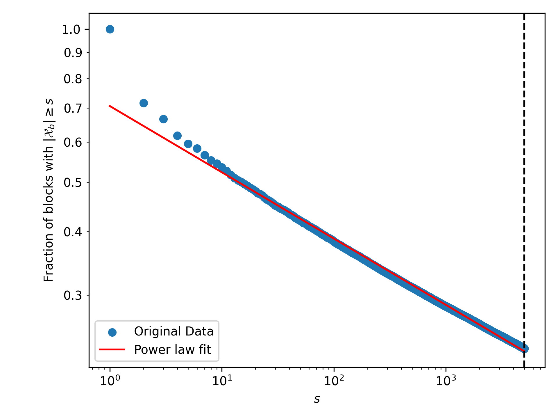
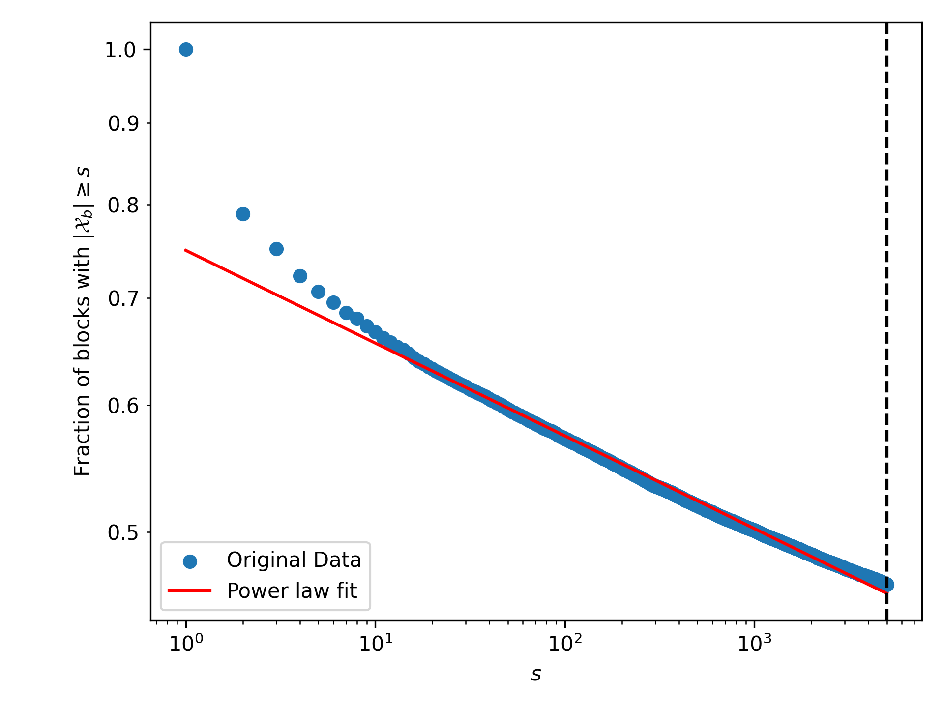
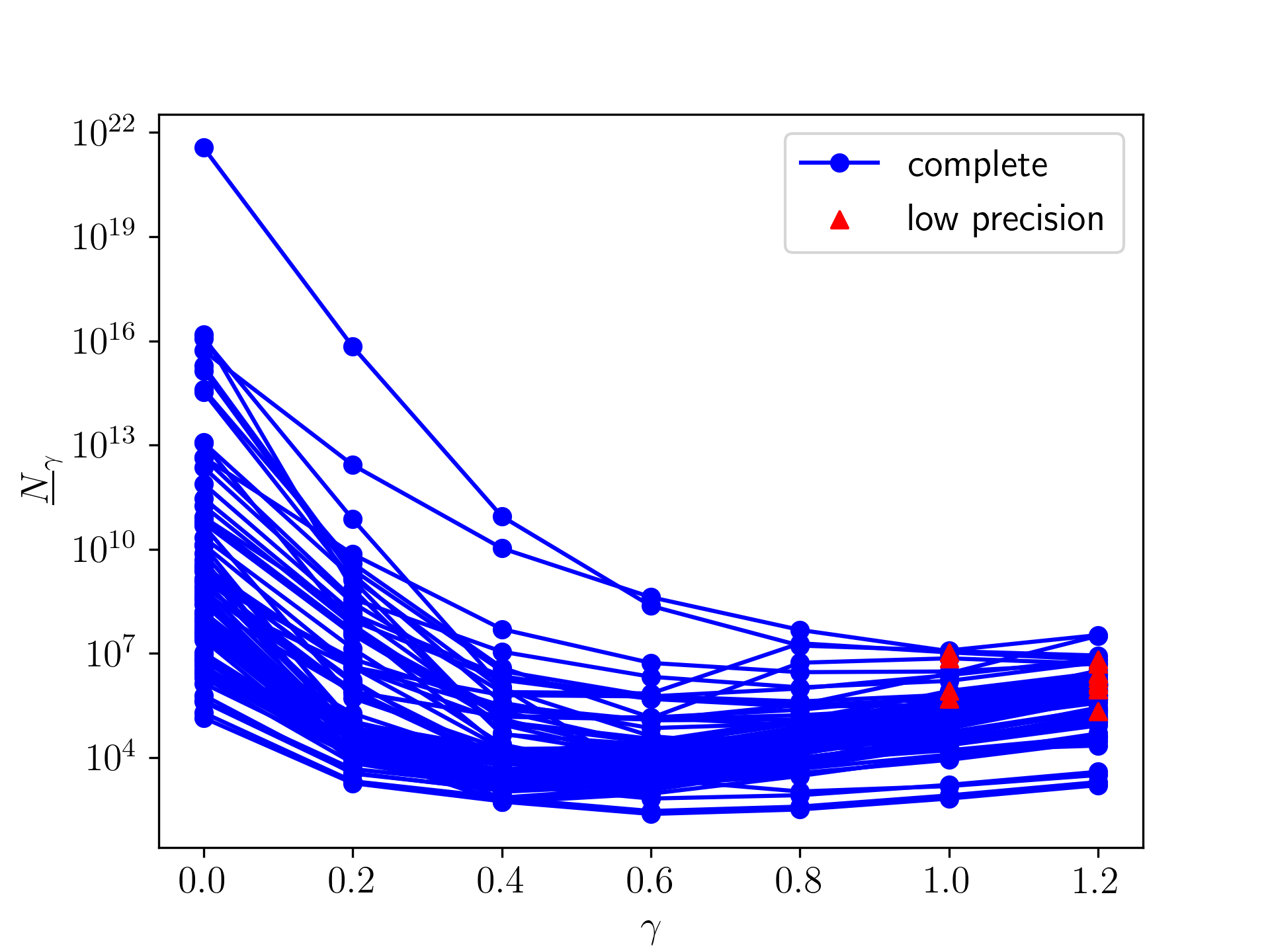
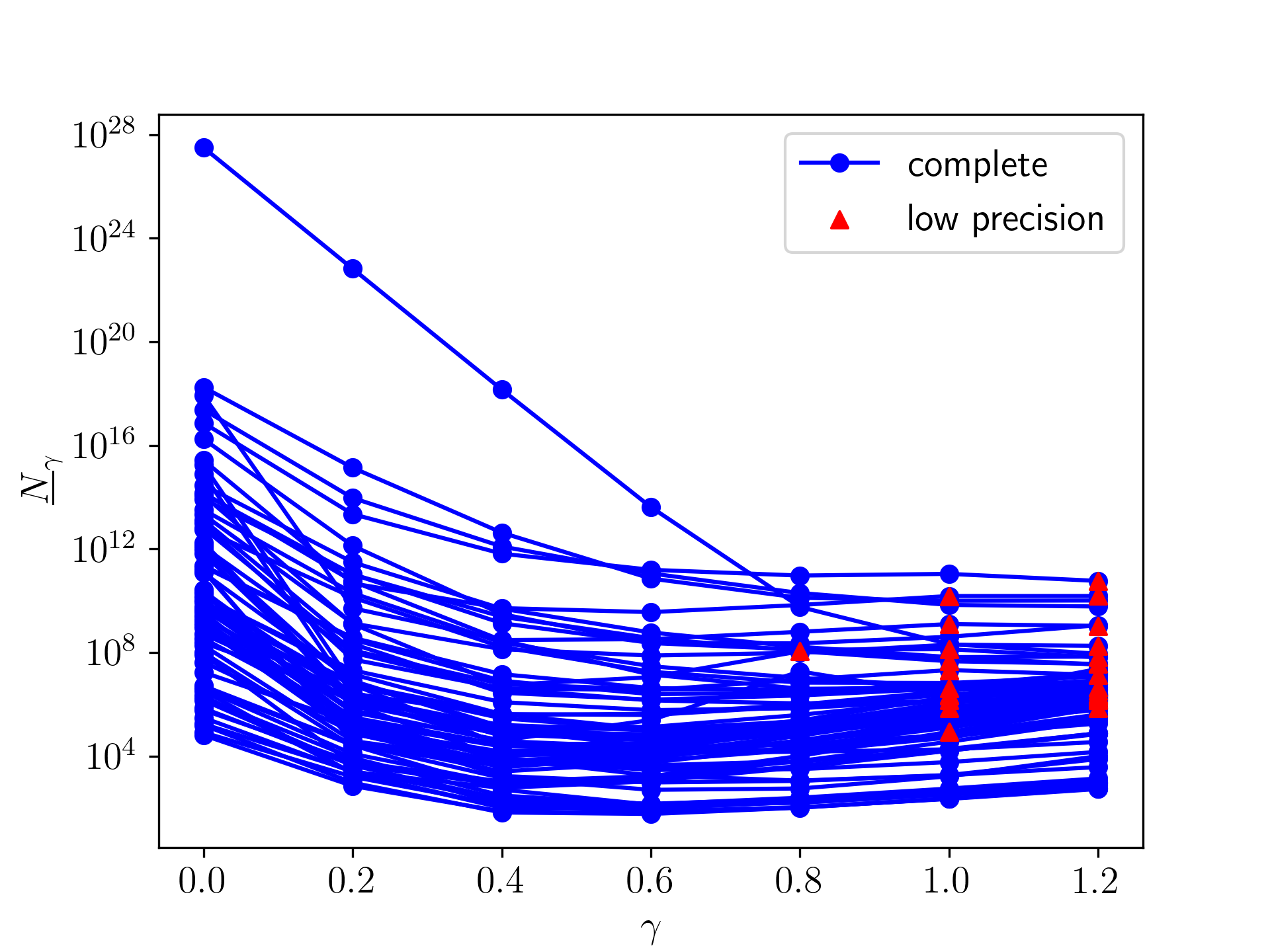
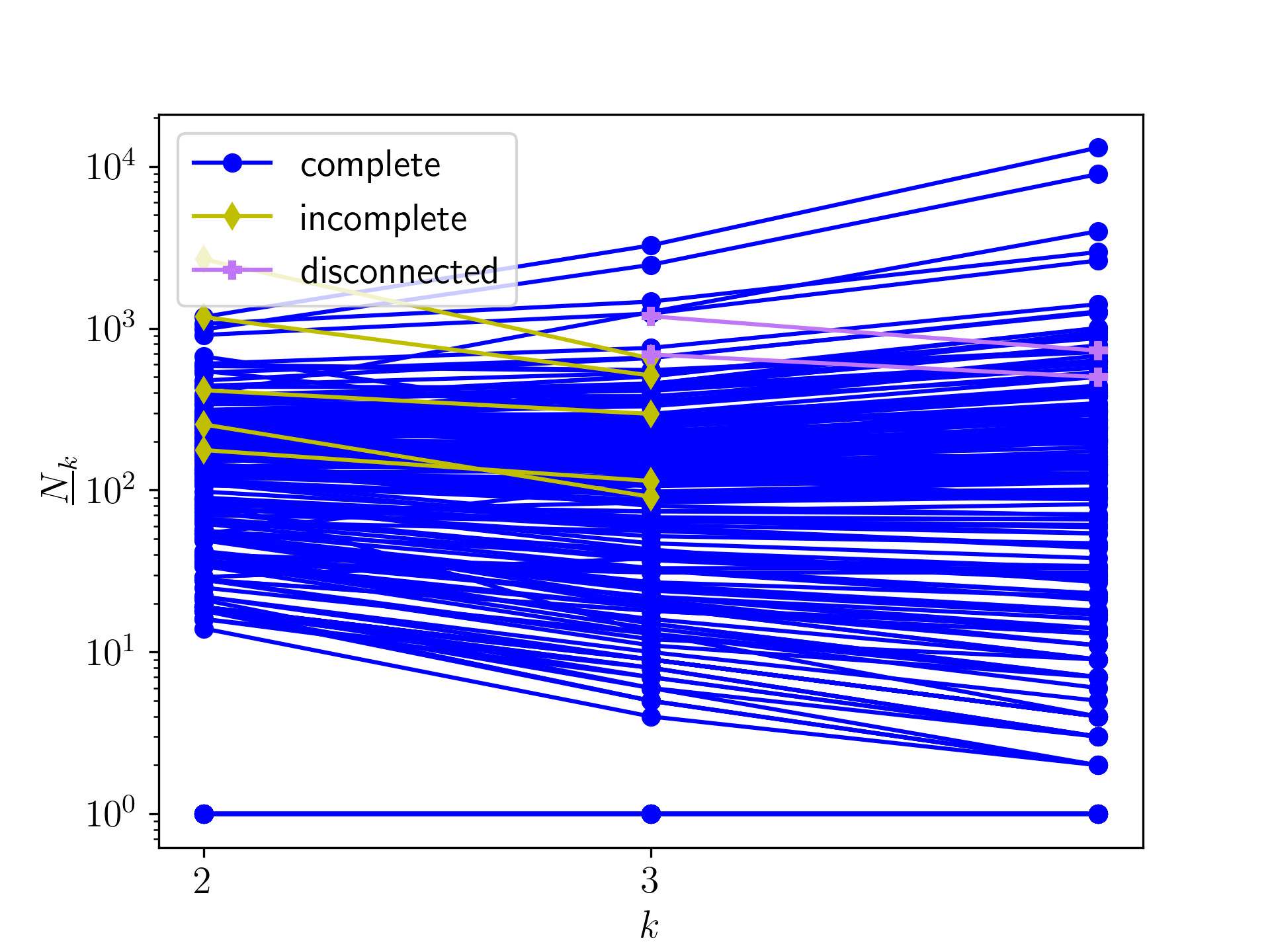
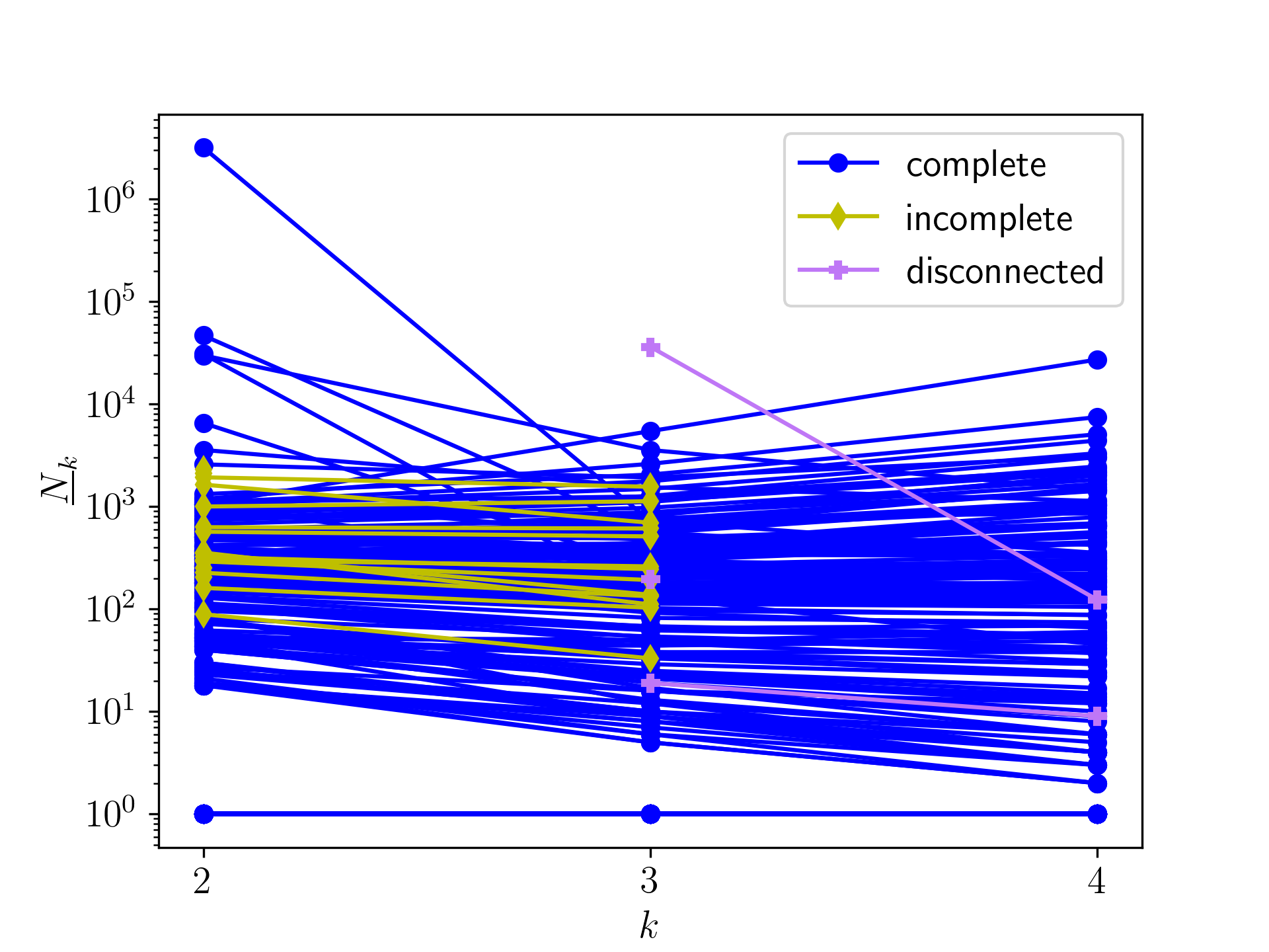
In addition to all of these techniques, we have one more tool at our disposal: Integer Linear Programming (ILP). For sufficiently small problems, we can use highly optimized software packages555We use Gurobi (https://www.gurobi.com/) in our experiments. for ILP to simply enumerate $\mathcal{X}$ and sample according to $\pi$ as desired. In all of our instances (where each instance is a Census block), we find that ILP suffices to determine whether $\mathcal{X}$ is non-empty. Enumeration, however, has a clear downside: its complexity scales with $|\mathcal{X}|$, which may be exponentially large in $n$, the number of possible households. For example, using ILP to enumerate up up to 5000 elements of $\mathcal{X}_{b}$ from each Census block in Alabama and Nevada, we plot the distribution of $\min(|\mathcal{X}_{b}|,5000)$ in Figure 1. Our results suggest that $|\mathcal{X}_{b}|$ has a heavy-tailed distribution,666We do not attempt to evaluate whether the power-law distribution fits these data well. Figures 1(a) and 1(b) are simply meant to be illustrative. meaning that enumerating $\mathcal{X}_{b}$ completely for each block is likely to be computationally infeasible.777For reference, enumerating up to 5000 solutions from $\mathcal{X}_{b}$ takes thousands of CPU-hours for Alabama and Nevada, which have 135,838 and 35,916 non-empty Census blocks respectively. For instances where $|\mathcal{X}_{b}|$ is too large, we need more efficient sampling algorithms. We turn to Markov Chain Monte Carlo methods for this.

Refer to caption
(a) AL
Refer to caption
(b) NV
Figure 1: $|\mathcal{X}_{b}|$ appears to be heavy-tailed.

4 Markov Chain Monte Carlo Methods

Markov Chain Monte Carlo methods can allow us to efficiently sample from exponentially large state spaces and have been used in prior work on knapsack sampling (Dyer et al., 1993; Morris and Sinclair, 2004). At a high level, MCMC works by defining a Markov chain over the solution space, performing a random walk on this Markov chain, and yielding a solution after a fixed number of random walk steps. Here, we develop MCMC techniques to solve MMS-Sample. We present two approaches: the “simple” chain, a modification of the algorithm of Dyer et al. (1993), and the “reduced” chain, which can be interpreted as a truncation of the simple chain. These come with trade-offs, which we evaluate both theoretically and empirically. At a high level, the simple chain is guaranteed to converge to the desired stationary distribution but may mix slowly. In contrast, the reduced chain may not converge to the desired distribution, but empirically performs better in our setting. Neither comes with strong theoretical guarantees; this is to be expected, since MMS-Sample is provably hard in the general case.

Preliminaries.

As is standard for MCMC, we will evaluate our algorithms in terms of the computation required to produce an approximately random sample from $\pi$ on $\mathcal{X}$. Define $d_{\mathrm{TV}}$ to be the total variation distance:

$\displaystyle d_{\mathrm{TV}}(\sigma,\sigma^{\prime})\triangleq\frac{1}{2}\|\sigma-\sigma^{\prime}\|_{1}=\max_{\mathcal{S}\subset\mathcal{X}}|\sigma(\mathcal{S})-\sigma^{\prime}(\mathcal{S})|.$ (2)

Let $\mathbb{X}$ denote a sample generated via MCMC, and let $\sigma_{\mathbb{X}}$ be its distribution. Our goal is to produce an $\varepsilon$-approximate sample from $\sigma$, i.e., we would like $\sigma_{\mathbb{X}}$ to satisfy $d_{\mathrm{TV}}(\sigma,\sigma_{\mathbb{X}})\leq\varepsilon$. This is closely related to the mixing time of a Markov chain with transition matrix $P$:

$\displaystyle\tau_{\mathrm{mix}}(\varepsilon;P)\triangleq\min\left\{t\in\mathbb{Z}_{\geq 0}:\max_{\sigma_{0}}d_{\mathrm{TV}}(\sigma_{0}P^{t},\sigma)\leq\varepsilon\right\}.$

However, because the algorithms we present each have a known initial state $\sigma_{0}$, we are not interested in the worst-case over all $\sigma_{0}$. Instead, we use a variant of the mixing time given a known starting distribution $\sigma_{0}$ with probability 1 on initial state $\mathbf{x}_{0}$ and 0 elsewhere. Define

$\displaystyle\tau_{\mathrm{mix}}(\varepsilon;P,\mathbf{x}_{0})\triangleq\min\left\{t\in\mathbb{Z}_{\geq 0}:d_{\mathrm{TV}}(\sigma_{0}P^{t},\sigma)\leq\varepsilon\right\}$ (3)

to be the number of iterations required to generate an $\varepsilon$-approximate sample from the stationary distribution $\sigma$. Standard spectral techniques yield bounds for $\tau_{\mathrm{mix}}(\varepsilon;P,\mathbf{x}_{0})$. Let $P$ be the transition matrix of an irreducible Markov chain. Assume that the chain is “lazy,” i.e., $P(\mathbf{x},\mathbf{x})\geq 1/2$ for all $\mathbf{x}$. Let $\lambda_{2}(P)$ be the second-largest eigenvalue of $P$. Then, the relaxation time of $P$ is defined as $\tau_{\mathrm{rel}}\triangleq\frac{1}{1-\lambda_{2}(P)}$. Classical results tell us that $\tau_{\mathrm{rel}}$ provides a tight characterization of $\tau_{\mathrm{mix}}(\varepsilon;P,\mathbf{x}_{0})$:

Theorem 1 (E.g., Guruswami (2016, Prop. 2.3); see also Levin et al. (2017, Thm. 12.5)).

For an irreducible, aperiodic Markov chain,

$\displaystyle\left(\tau_{\mathrm{rel}}-1\right)\log\left(\frac{1}{2\varepsilon}\right)\leq\tau_{\mathrm{mix}}(\varepsilon;P,\mathbf{x}_{0})\leq\tau_{\mathrm{rel}}\log\left(\frac{1}{\varepsilon\sigma(\mathbf{x}_{0})}\right).$ (4)

Next, we describe and analyze our two MCMC-based algorithms.

4.1 The simple chain

4.1.1 Defining the simple chain

We begin by adapting the algorithm of Dyer et al. (1993) which samples uniformly from the set of feasible knapsack solutions $\mathcal{Y}\triangleq\{\mathbf{x}:\mathbf{V}\mathbf{x}\preceq\mathbf{c}\}$. Our adaptation has two key differences: we are interested in exact solutions (i.e., $\mathcal{X}=\{\mathbf{x}:\mathbf{V}\mathbf{x}=\mathbf{c}\}$), and we want to sample from a particular distribution $\pi$ as defined in 1. We design a Markov chain $M_{\gamma}$ parameterized by $\gamma\in\mathbb{R}$ with stationary distribution $\tilde{\pi}_{\gamma}$:

$\displaystyle\tilde{\pi}_{\gamma}(\mathbf{x})\propto f(\mathbf{x})\exp(-\gamma\|\mathbf{V}\mathbf{x}-\mathbf{c}\|_{1})$ (5)

over $\mathcal{Y}$. Observe that the conditional distribution of $\tilde{\pi}_{\gamma}$ over $\mathcal{X}$ is $\pi$, i.e., $(\tilde{\pi}_{\gamma}\;|\;\mathbf{x}\in\mathcal{X})=\pi$. As a result, if we can sample efficiently from $\tilde{\pi}_{\gamma}$, we can use rejection sampling to generate samples from $\pi$ over $\mathcal{X}$. In other words, our plan will be to repeatedly generate samples from $\mathcal{Y}$ according to $\tilde{\pi}_{\gamma}$ and accept the first sample that happens to lie in $\mathcal{X}$. Our choice of $\tilde{\pi}_{\gamma}$ to penalize lower-quality solutions is a standard technique (see, e.g., Porod (2024)), and $\gamma$ is often referred to as an “inverse temperature” parameter. We next specify a Markov chain with stationary distribution $\tilde{\pi}_{\gamma}$.

Let $h(\mathbf{x},\mathbf{x}^{\prime})$ denote the number of entries in which $\mathbf{x}$ and $\mathbf{x}^{\prime}$ disagree (i.e., $h(\mathbf{x},\mathbf{x}^{\prime})\triangleq\|\mathbf{x}-\mathbf{x}^{\prime}\|_{\infty}$). For $\mathbf{x},\mathbf{x}^{\prime}\in\mathcal{Y}$ such that $h(\mathbf{x},\mathbf{x}^{\prime})=1$, let $\delta(\mathbf{x},\mathbf{x}^{\prime})$ be the index $i$ on which they disagree, so $\mathbf{x}[i]\neq\mathbf{x}^{\prime}[i]$. Finally, let $\Delta(\mathbf{x},i)\triangleq\{\mathbf{x}_{i\leftarrow g}:\mathbf{V}\mathbf{x}_{i\leftarrow g}\preceq\mathbf{c},~{}g\in\mathbb{Z}_{\geq 0}\}$. (Recall that $\mathbf{x}_{i\leftarrow g}$ denotes replacing the $i$th entry of $\mathbf{x}$ with the value $g$.) Intuitively, $\Delta(\mathbf{x},i)$ yields the set of feasible knapsack solutions obtained by changing the $i$th entry of $\mathbf{x}$ to some other nonnegative integer $g$. Our Markov chain $M_{\gamma}$ defined on the state space $\mathcal{Y}$ uses Gibbs sampling, with transition probabilities

$\displaystyle P_{\gamma}(\mathbf{x},\mathbf{x}^{\prime})\triangleq\begin{cases}\frac{\tilde{\pi}_{\gamma}(\mathbf{x}^{\prime})}{2n\sum_{\mathbf{x}^{\prime\prime}\in\Delta(\mathbf{x},i)}\tilde{\pi}_{\gamma}(\mathbf{x}^{\prime\prime})}&h(\mathbf{x},\mathbf{x}^{\prime})=1\wedge\delta(\mathbf{x},\mathbf{x}^{\prime})=i\\ 0&h(\mathbf{x},\mathbf{x}^{\prime})>1\\ 1-\sum_{\mathbf{x}^{\prime\prime}\neq\mathbf{x}}P_{\gamma}(\mathbf{x},\mathbf{x}^{\prime\prime})&\mathbf{x}=\mathbf{x}^{\prime}\end{cases}$

4.1.2 Properties of the simple chain

In order to show that we running MCMC on $M_{\gamma}$ yields an approximate sample from $\tilde{\pi}_{\gamma}$, we will show that:

  • $M_{\gamma}$ is lazy and irreducible.

  • The stationary distribution of $M_{\gamma}$ is $\tilde{\pi}_{\gamma}$.

  • We can implement the transitions $P_{\gamma}$ with an efficient algorithm.

First, observe that by construction, $M_{\gamma}$ is “lazy,” meaning $P_{\gamma}(\mathbf{x},\mathbf{x})\geq 1/2$. This is because

$\displaystyle P_{\gamma}(\mathbf{x},\mathbf{x})$ $\displaystyle=1-\sum_{\mathbf{x}^{\prime}\neq\mathbf{x}}P_{\gamma}(\mathbf{x},\mathbf{x}^{\prime})$
$\displaystyle=1-\sum_{i=1}^{n}\sum_{\mathbf{x}^{\prime}\in\Delta(\mathbf{x},i)\backslash\{\mathbf{x}\}}\frac{\tilde{\pi}_{\gamma}(\mathbf{x}^{\prime})}{2n\sum_{\mathbf{x}^{\prime\prime}\in\Delta(\mathbf{x},i)}\tilde{\pi}_{\gamma}(\mathbf{x}^{\prime\prime})}$
$\displaystyle\geq 1-\sum_{i=1}^{n}\sum_{\mathbf{x}^{\prime}\in\Delta(\mathbf{x},i)}\frac{\tilde{\pi}_{\gamma}(\mathbf{x}^{\prime})}{2n\sum_{\mathbf{x}^{\prime\prime}\in\Delta(\mathbf{x},i)}\tilde{\pi}_{\gamma}(\mathbf{x}^{\prime\prime})}$
$\displaystyle=\frac{1}{2}$

Moreover, any state is reachable from any other state since all states are connected to the empty solution $\mathbf{x}=\mathbf{0}$. This guarantees that $M_{\gamma}$ is aperiodic and $P_{\gamma}$ has nonnegative eigenvalues.

Next, we will show that $\tilde{\pi}_{\gamma}$ is the stationary distribution of $M_{\gamma}$. For an aperiodic, irreducible Markov chain, a distribution $\sigma$ that satisfies the so-called “detailed balance equations” given by 6 is its unique stationary distribution (see, e.g., Levin et al. (2017, Cor. 1.17 and Prop. 1.20)):

$\displaystyle\sigma(\mathbf{x})P(\mathbf{x},\mathbf{x}^{\prime})=\sigma(\mathbf{x}^{\prime})P(\mathbf{x}^{\prime},\mathbf{x}).$ (6)

In our case, this is clearly true for $\mathbf{x}=\mathbf{x}^{\prime}$ and when $h(\mathbf{x},\mathbf{x}^{\prime})>1$ (since $P_{\gamma}(\mathbf{x},\mathbf{x}^{\prime})=P_{\gamma}(\mathbf{x}^{\prime},\mathbf{x})=0$ in this case). For $h(\mathbf{x},\mathbf{x}^{\prime})=1$, let $i=\delta(\mathbf{x},\mathbf{x}^{\prime})$. Note that $\Delta(\mathbf{x},i)=\Delta(\mathbf{x}^{\prime},i)$ by construction. Therefore,

$\displaystyle\tilde{\pi}_{\gamma}(\mathbf{x})P_{\gamma}(\mathbf{x},\mathbf{x}^{\prime})$ $\displaystyle=\frac{\tilde{\pi}_{\gamma}(\mathbf{x})\tilde{\pi}_{\gamma}(\mathbf{x}^{\prime})}{2n\sum_{\mathbf{x}^{\prime\prime}\in\Delta(\mathbf{x},i)}\tilde{\pi}_{\gamma}(\mathbf{x}^{\prime\prime})}=\frac{\tilde{\pi}_{\gamma}(\mathbf{x})\tilde{\pi}_{\gamma}(\mathbf{x}^{\prime})}{2n\sum_{\mathbf{x}^{\prime\prime}\in\Delta(\mathbf{x}^{\prime},i)}\tilde{\pi}_{\gamma}(\mathbf{x}^{\prime\prime})}=\tilde{\pi}_{\gamma}(\mathbf{x}^{\prime})P_{\gamma}(\mathbf{x}^{\prime},\mathbf{x}).$

Thus, $\tilde{\pi}_{\gamma}$ is the stationary distribution of $M_{\gamma}$.

Finally, we must show that given $\mathbf{x}$, we can efficiently sample from $P_{\gamma}(\mathbf{x},\cdot)$. The following algorithm does so: with probability $1/2$, remain at $\mathbf{x}$. With the remaining probability $1/2$ choose a $i\in[n]$ uniformly at random and enumerate the set $\Delta(\mathbf{x},i)$. (In our instances, entries of $\mathbf{c}$ are on the order of thousands at most, meaning $|\Delta(\mathbf{x},i)|$ is relatively small, and this can be done through binary search.) Then, sample $\mathbf{x}^{\prime}$ proportional to $\tilde{\pi}_{\gamma}(\cdot)$ from $\Delta(\mathbf{x},i)$ and transition to $\mathbf{x}^{\prime}$. We formally describe this in Algorithm 2 in Section C.1.

4.1.3 The number of samples needed for rejection sampling

To generate a sample from $\mathcal{X}$ (not just from $\mathcal{Y}\supset\mathcal{X}$), given some hyperparameter $t$, we run $M_{\gamma}$ for $t$ iterations beginning with the empty solution as the start state (i.e., $\mathbf{x}_{0}=\mathbf{0}$).888When we evaluate the simple chain, the starting state will not matter for the lower bounds we show. This yields a sample $\mathbf{x}\sim\pi_{\gamma,t}$, where we define $\pi_{\gamma,t}\triangleq\pi_{0}P_{\gamma}^{t}$ to be the distribution of the random walk after $t$ steps. If $\mathbf{x}\in\mathcal{X}$, then we return $\mathbf{x}$; if not, we repeat the process until we find some $\mathbf{x}\in\mathcal{X}$. See Algorithm 2 for details.

Define $p_{\gamma}(t)\triangleq\pi_{\gamma,t}(\mathcal{X})=\Pr_{\mathbb{X}\sim\pi_{\gamma,t}}[\mathbb{X}\in\mathcal{X}]$ to be the probability that a sample from $\pi_{\gamma,t}$ is in $\mathcal{X}$. Because the number of samples needed for rejection sampling is geometrically distributed with parameter $p_{\gamma}(t)$, the total expected number of Markov chain iterations to produce a sample from $\mathcal{X}$ is $t/p_{\gamma}(t)$. To fully specify our algorithm, we must choose $t$ to be sufficiently large to produce an $\varepsilon$-approximate sample from $\mathcal{X}$.

For the simple chain, we might think that it suffices to choose $t\geq\tau_{\mathrm{mix}}(\varepsilon;P_{\gamma},\mathbf{x}_{0})$, since this implies that $d_{\mathrm{TV}}(\pi_{\gamma,t},\tilde{\pi}_{\gamma})\leq\varepsilon$. However, this is insufficient: We want an $\varepsilon$-approximate sample from $\mathcal{X}$, not from $\mathcal{Y}$. Roughly speaking, a sample with approximation error $\varepsilon$ for $\tilde{\pi}_{\gamma}$ may have approximation error on the order $\varepsilon/\tilde{\pi}_{\gamma}(\mathcal{X})$ on $\mathcal{X}$. We formalize this in Lemma 2, which we prove in Section C.2.

Lemma 2.

Let $\sigma$ and $\sigma^{\prime}$ be distributions defined on $\mathcal{Y}$. Let $\sigma_{\mathcal{X}}$ and $\sigma_{\mathcal{X}}^{\prime}$ be their conditional distributions on $\mathcal{X}\subset\mathcal{Y}$, i.e., for $\mathbf{x}\in\mathcal{X}$, $\sigma_{\mathcal{X}}(\mathbf{x})=\sigma(\mathbf{x})/\sigma(\mathcal{X})$. If $d_{\mathrm{TV}}(\sigma,\sigma^{\prime})\leq\varepsilon$, then $d_{\mathrm{TV}}(\sigma_{\mathcal{X}},\sigma_{\mathcal{X}}^{\prime})\leq 3\varepsilon/(2\sigma(\mathcal{X}))$. For any $\varepsilon$, there exist instances for which this is tight to within a constant factor.

Let $p_{\gamma}^{*}\triangleq\lim_{t\to\infty}p_{\gamma}(t)=\tilde{\pi}_{\gamma}(\mathcal{X})$. By Lemma 2, to generate an $\varepsilon$-approximate sample from $\mathcal{X}$, it suffices to choose $t\geq t^{*}_{\gamma}(\varepsilon)\triangleq\tau_{\mathrm{mix}}(2p_{\gamma}^{*}\varepsilon/3;P_{\gamma},\mathbf{x}_{0})$, since

$\displaystyle d_{\mathrm{TV}}(\pi_{\gamma,t}\;|\;\mathbf{x}\in\mathcal{X},\tilde{\pi}_{\gamma}\;|\;\mathbf{x}\in\mathcal{X})\leq\frac{3d_{\mathrm{TV}}(\pi_{\gamma,t},\tilde{\pi}_{\gamma})}{2\tilde{\pi}_{\gamma}(\mathcal{X})}\leq\frac{3(2p_{\gamma}^{*}\varepsilon/3)}{2p_{\gamma}^{*}}=\varepsilon.$

In other words, a $2p_{\gamma}^{*}\varepsilon/3$-approximate sample from $\tilde{\pi}_{\gamma}$ over $\mathcal{Y}$ yields an $\varepsilon$-approximate sample on from $\pi$ over $\mathcal{X}$. This is tight to within a constant factor. Of course, we know neither $p_{\gamma}^{*}$ nor $\tau_{\mathrm{mix}}(\cdot;P_{\gamma},\mathbf{x}_{0})$ a priori; we experimentally determine them for our instances in Section 4.1.4. With this choice of $t$, the expected number of MCMC iterations needed to produce an $\varepsilon$-approximate sample from $\mathcal{X}$ is

$\displaystyle N_{\gamma}(\varepsilon)\triangleq\frac{t^{*}_{\gamma}(\varepsilon)}{p_{\gamma}(t^{*}_{\gamma}(\varepsilon))}.$ (7)

4.1.4 Empirical results for the simple chain

To evaluate the performance of Algorithm 2, our goal will be to determine $N_{\gamma}(\varepsilon)$ for our instances. To do so, we will bound both $t^{*}_{\gamma}(\varepsilon)$ and $p_{\gamma}(t^{*}_{\gamma}(\varepsilon))$. Observe that because $d_{\mathrm{TV}}(\pi_{\gamma,t^{*}_{\gamma}(\varepsilon)},\tilde{\pi}_{\gamma})\leq 2p_{\gamma}^{*}\varepsilon/3$, by definition of total variation distance 2,

$\displaystyle\left(1-\frac{2\varepsilon}{3}\right)p_{\gamma}^{*}\leq p_{\gamma}(t^{*}_{\gamma}(\varepsilon))\leq\left(1+\frac{2\varepsilon}{3}\right)p_{\gamma}^{*}.$ (8)

Let $\tau_{\mathrm{rel},\gamma}\triangleq\frac{1}{1-\lambda_{2}(P_{\gamma})}$ be the relaxation time of $M_{\gamma}$. Combining 4 and 8 yields

$\displaystyle\underline{N}_{\gamma}(\varepsilon)\triangleq\frac{(\tau_{\mathrm{rel},\gamma}-1)\log\left(\frac{3}{4\varepsilon p_{\gamma}^{*}}\right)}{\left(1+\frac{2\varepsilon}{3}\right)p_{\gamma}^{*}}\leq N_{\gamma}(\varepsilon)\leq\frac{\tau_{\mathrm{rel},\gamma}\log\left(\frac{3}{2\varepsilon p_{\gamma}^{*}\tilde{\pi}_{\gamma}(\mathbf{x}_{0})}\right)}{\left(1-\frac{2\varepsilon}{3}\right)p_{\gamma}^{*}}\triangleq\overline{N}_{\gamma}(\varepsilon).$ (9)

We will use these tight lower and upper bounds for $N_{\gamma}(\varepsilon)$ to characterize the performance of the simple chain. We choose $\varepsilon=1/(2e)$ by convention and write $N_{\gamma}=N_{\gamma}(1/(2e))$.

Refer to caption
(a) AL
Refer to caption
(b) NV
Figure 2: There are blocks for which the number of iterations required to generate an $\varepsilon$-approximate sample from $\mathcal{X}$ using the simple chain is large. The reduced chain (described in Section 4.2) requires orders of magnitude fewer iterations in the worst case.

Computing $\underline{N}_{\gamma}$ requires $\Omega(|\mathcal{Y}|)$ time and space, which can be prohibitive for our instances (i.e., Census blocks) since $\mathcal{Y}$ can be exponentially large. Our approach is as follows: we choose a subset of “small” instances and compute the full transition matrix $P_{\gamma}$ for a random sample of those instances. We will show that in this sample, there exist instances for which $\underline{N}_{\gamma}$ is prohibitively large, making Algorithm 2 impractical in our setting.
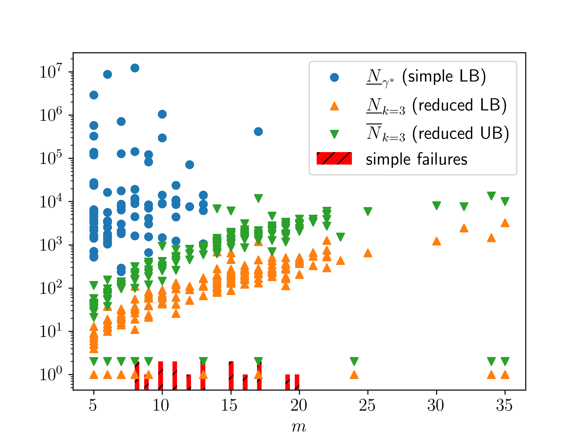
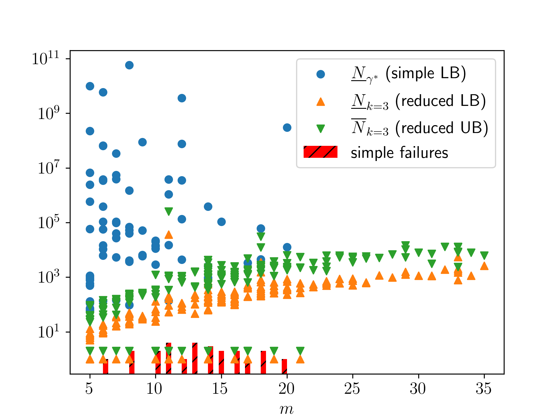
Recall that $m$ is the number of households in a Census block. We sample 100 blocks where $5\leq m\leq 20$ and $|\mathcal{X}|<5000$ in two states: Alabama and Nevada (chosen arbitrarily). For each block, we seek to compute $P_{\gamma}$ for $\gamma\in\Gamma\triangleq\{0.0,0.2,0.4,0.6,0.8,1.0,1.2\}$. For a significant number of blocks (indicated on Figure 2 in red bars; 25 in NV and 17 in AL), we fail to compute $P_{\gamma}$ within a time limit of 8 hours. In Appendix E, we show that the globally optimal choice for $\gamma$ on our sample is $\approx 0.8$.999Due to numerical instability in computing eigenvalues of $P_{\gamma}$, we sometimes underestimate $\underline{N}_{\gamma}$ for larger values of $\gamma$.

In Figure 2, we plot $\underline{N}_{\gamma^{*}}$ for the blocks in our sample, where for each block, $\underline{N}_{\gamma^{*}}\triangleq\min_{\gamma\in\Gamma}\underline{N}_{\gamma}$ using blue $\CIRCLE$ markers. (This is simply taking the “best” choice of $\gamma$ for each block.) Observe that $\underline{N}_{\gamma^{*}}$ can be quite large, even for small instances. There are blocks with fewer than 10 households for which $\underline{N}_{\gamma^{*}}$ is on the order of $10^{11}$. In contrast, the “reduced” approach we develop in Section 4.2 appears to perform much better: the analogous lower and upper bounds for the reduced chain are small for all of our instances (Figure 2, orange $\blacktriangle$ and green $\blacktriangle$ markers respectively).101010While we compare MCMC iterations as opposed to computation time here, our experiments show that computation time per iteration is similar for the two. See Appendix E for details.

4.1.5 Theoretical results for the simple chain

Before we describe this improved approach, we briefly provide a theoretical characterization of how $\underline{N}_{\gamma}$ varies with $\gamma$ to gain some intuition as to why the simple chain performs poorly and how $N_{\gamma}$ depends on $\gamma$. Intuitively, we will see that varying $\gamma$ creates a trade-off between $p_{\gamma}^{*}$ and $\tau_{\mathrm{rel},\gamma}$. (Recall that $\tau_{\mathrm{rel},\gamma}$ is the relaxation time of $M_{\gamma}$.) Since $N_{\gamma}\approx\tau_{\mathrm{rel},\gamma}/p_{\gamma}^{*}$, these opposing forces empirically make the simple chain impractical in our setting.

We begin by characterizing how $p_{\gamma}^{*}$ varies with $\gamma$. All proofs are deferred to Section C.2.

Lemma 3.

$p_{\gamma}^{*}$ is monotonically increasing in $\gamma$, and

$\displaystyle\lim_{\gamma\to-\infty}p_{\gamma}^{*}=0$ and $\displaystyle\lim_{\gamma\to\infty}p_{\gamma}^{*}=1$

As a result, large values of $\gamma$ make it more likely that we sample an exact solution $\mathbf{x}\in\mathcal{X}$. Unfortunately, this comes at a cost, which we show in Lemma 4: in the limit, as $\gamma$ increases, $\tau_{\mathrm{rel},\gamma}$ increases exponentially.111111A stronger version of this result would claim that, analogously to Lemma 3, mixing time increases monotonically with $\gamma$. While this may be true, proving monotonicity over the temperature parameter is notoriously difficult (see, e.g., Nacu (2003); Kargin (2011) and Levin et al. (2017, Ch. 26 Open Question 2)).

Lemma 4.

For the stationary distribution $\tilde{\pi}_{\gamma}$ as defined in 5, $\tau_{\mathrm{rel},\gamma}=\Omega(\exp(\gamma\min_{i}\|\mathbf{v}_{i}\|_{1}))$.

We use a conductance argument and Cheeger’s inequality (Lawler and Sokal, 1988; Jerrum and Sinclair, 1988) to prove this. Taken together, Lemmas 3 and 4 describe the trade-off in our choice of $\gamma$: for small values of $\gamma$, samples from $\tilde{\pi}_{\gamma}$ rarely fall in $\mathcal{X}$, making rejection sampling inefficient. For large values of $\gamma$, the mixing time of the simple chain increases exponentially, requiring many iterations to generate each sample. These results tell us that the optimal choice of $\gamma$ is finite.

Lemma 5.

For every instance, there is some finite $\gamma$ that minimizes $N_{\gamma}$.

Figure 3 visualizes this trade-off. Each line represents a different Census block. Red triangle $\blacktriangle$ markers show low-precision estimates for the spectral gap, which will typically mean we underestimate $\underline{N}_{\gamma}$. Observe that each line appears to be quasiconvex, with a minimum in our range of choices for $\gamma$.

Refer to caption
(a) AL
Refer to caption
(b) NV
Figure 3: $\underline{N}_{\gamma}$ as a function of $\gamma$.

4.2 The reduced chain

Part of the reason why Algorithm 2 requires many iterations in expectation to produce a valid sample from $\mathcal{X}$ is its potentially large state space: because $\mathcal{Y}$ can be much larger than $\mathcal{X}$, a random walk according to $P_{\gamma}$ may yield samples from $\mathcal{Y}\backslash\mathcal{X}$ with very high probability. This motivates our approach: the “reduced” chain. We design a Markov chain $M_{k}$ with state space $\mathcal{X}$ instead of $\mathcal{Y}$.

4.2.1 Defining the reduced chain

The reduced chain is parameterized by an integer $k\geq 2$. Intuitively, given a solution $\mathbf{x}\in\mathcal{X}$, we randomly remove $k$ elements and replace them with another multiset of $k$ elements (found via ILP) such that the resulting sum still exactly equals the constraint $\mathbf{c}$. For small $k$, this can be done fairly quickly. In our experiments, we use $k\in\{2,3,4\}$.

We again use a variant of Gibbs sampling to induce the desired stationary distribution. We define the following transition matrix $P_{k}$ for our Markov chain $M_{k}$. Let $\mathcal{A}(\mathbf{x},\mathbf{x}^{\prime})$ be the set of distinct pairs of multisets $(\mathbf{z},\mathbf{z}^{\prime})$, each of size $k$, such that we can transform $\mathbf{x}$ into $\mathbf{x}^{\prime}$ by removing elements from $\mathbf{z}$ and replacing them with elements from $\mathbf{z}^{\prime}$. Formally, this is

$\displaystyle\mathcal{A}(\mathbf{x},\mathbf{x}^{\prime})\triangleq\{(\mathbf{z},\mathbf{z}^{\prime})\in\mathbb{Z}_{\geq 0}^{n}\times\mathbb{Z}_{\geq 0}^{n}:(\mathbf{V}\mathbf{z}=\mathbf{V}\mathbf{z}^{\prime})\wedge(\mathbf{x}-\mathbf{z}=\mathbf{x}^{\prime}-\mathbf{z}^{\prime}\succeq\mathbf{0})\wedge(\|\mathbf{z}\|_{1}=\|\mathbf{z}^{\prime}\|_{1}=k)\}.$

Let $\mathcal{Z}(\mathbf{z})\triangleq\{\mathbf{z}^{\prime}\in\mathbb{Z}_{\geq 0}^{n}:(\mathbf{V}\mathbf{z}^{\prime}=\mathbf{V}\mathbf{z})\wedge(\mathbf{z}^{\prime}\succeq\mathbf{0})\}$. Then, for $\mathbf{x},\mathbf{x}^{\prime}\in\mathcal{X}$,121212Because the elements in $\mathcal{V}$ are unique, it is impossible to have $h(\mathbf{x},\mathbf{x}^{\prime})=1$ for $\mathbf{x},\mathbf{x}^{\prime}\in\mathcal{X}$.

$\displaystyle P_{k}(\mathbf{x},\mathbf{x}^{\prime})\triangleq\begin{cases}\frac{1}{2\binom{m}{k}}\sum_{(\mathbf{z},\mathbf{z}^{\prime})\in\mathcal{A}(\mathbf{x},\mathbf{x}^{\prime})}\frac{\pi(\mathbf{x}^{\prime})}{\sum_{\mathbf{z}^{\prime\prime}\in\mathcal{Z}(\mathbf{z})}\pi(\mathbf{x}-\mathbf{z}+\mathbf{z}^{\prime\prime})}&2\leq h(\mathbf{x},\mathbf{x}^{\prime})\leq 2k\\ 0&h(\mathbf{x},\mathbf{x}^{\prime})>2k\\ 1-\sum_{\mathbf{x}^{\prime\prime}\neq\mathbf{x}}P_{k}(\mathbf{x},\mathbf{x}^{\prime\prime})&\mathbf{x}=\mathbf{x}^{\prime}\end{cases}.$

Because $\mathcal{Z}(\mathbf{z})=\mathcal{Z}(\mathbf{z}^{\prime})$ for $(\mathbf{z},\mathbf{z}^{\prime})\in\mathcal{A}(\mathbf{x},\mathbf{x}^{\prime})$, $\pi$ satisfies the detailed balance conditions $\pi(\mathbf{x})P_{k}(\mathbf{x},\mathbf{x}^{\prime})=\pi(\mathbf{x}^{\prime})P_{k}(\mathbf{x}^{\prime},\mathbf{x})$, making it a stationary distribution of $M_{k}$. Unfortunately, $\pi$ is not necessarily the unique stationary distribution of $M_{k}$, which we will discuss below. Note that $P_{k}$ is lazy by construction. In Algorithm 3 in Section D.1, we show that we can sample efficiently from $P_{k}(\mathbf{x},\cdot)$ as long as we can efficiently compute $\mathcal{Z}(\mathbf{z})$ (via ILP), which empirically we can in our setting. The complexity of this computation depends on the problem dimension $d$ and the parameter choice $k$, not on the total counts $\mathbf{c}$ or the problem size $n$.

Choosing an initial state $\mathbf{x}_{0}$.

To fully specify the algorithm, we must choose an initial state $\mathbf{x}_{0}$. In general, we could find an arbitrary $\mathbf{x}_{0}\in\mathcal{X}$ via ILP; however, in order to produce tighter bounds on performance, we aim to begin with a “better-than-average” $\mathbf{x}_{0}$ (i.e., such that $\pi(\mathbf{x}_{0})\geq 1/|\mathcal{X}|$). To see why, observe that the upper bounds in 4 depend on $\log(1/\pi(\mathbf{x}_{0}))$, so larger values of $\pi(\mathbf{x}_{0})$ will reduce the number of MCMC iterations we need to produce a sample. We defer these details to Section D.1. Note that finding any $\mathbf{x}_{0}\in\mathcal{X}$ requires that we can solve the decision problem MMS via ILP despite its NP-hardness; empirically, we can for all of our instances.

The reduced chain is not necessarily irreducible.

In an irreducible Markov chain, any state is reachable from any other state, i.e., for any $\mathbf{x},\mathbf{x}^{\prime}\in\mathcal{X}$, there exists $t$ such that $P^{t}(\mathbf{x},\mathbf{x}^{\prime})>0$. This is not necessarily the case for $P_{k}$: it is possible to have disconnected components in the state space graph (see Figure 8 for an example). When this happens, $\pi$ is not the only stationary distribution of $M_{k}$, and our algorithm will not sample from $\pi$ as desired. We evaluate whether this is the case for our instances in what follows.

4.2.2 Empirical results for the reduced chain

We are interested in $N_{k}(\varepsilon)\triangleq\tau_{\mathrm{mix}}(\varepsilon;P_{k},\mathbf{x}_{0})$, defined to be the number of Markov chain iterations required to generate an $\varepsilon$-approximate sample from $\mathcal{X}$. If $M_{k}$ is not irreducible, $N_{k}(\varepsilon)$ is undefined. As in Section 4.1.4, we derive bounds for $N_{k}(\varepsilon)$ and evaluate these bounds for a random sample of instances. For irreducible $M_{k}$, let $\tau_{\mathrm{rel},k}\triangleq\frac{1}{1-\lambda_{2}(P_{k})}$. Using 4,

$\displaystyle\underline{N}_{k}(\varepsilon)\triangleq(\tau_{\mathrm{rel},k}-1)\log\left(\frac{1}{2\varepsilon}\right)\leq N_{k}(\varepsilon)\leq\tau_{\mathrm{rel},k}\log\left(\frac{1}{\varepsilon\pi(\mathbf{x}_{0})}\right)\triangleq\overline{N}_{k}(\varepsilon).$ (10)

We again choose $\varepsilon=1/(2e)$. Because our choice of $\mathbf{x}_{0}$ satisfies $\pi(\mathbf{x}_{0})\geq 1/|\mathcal{X}|$, the lower and upper bounds for are within $O(\log|\mathcal{X}|)$ of one another. In Lemma 6 in Section 4.2.3, we show that $\log|\mathcal{X}|=O(m\log n)$, meaning $N_{k}=O(\tau_{\mathrm{rel},k}\cdot m\log n)$ (see Corollary 1 below).

We re-use the same sample of 100 blocks per state that we used to evaluate the simple chain in Section 4.1.4. In addition, because $|\mathcal{X}|$ can be much smaller than $|\mathcal{Y}|$, we are able to compute $P_{k}$ for larger instances. We therefore sample another 100 blocks for each of AL and NV with $14\leq m\leq 35$ and $|\mathcal{X}|<5000$.131313In Alabama and Nevada, 72% and 45% of blocks respectively have $m\leq 35$, $|\mathcal{X}|<5000$, and sufficiently consistent data for our use (see Appendix A for details about excluded blocks). For each block, we analyze $k\in\{2,3,4\}$.141414For some blocks, our computation times out (beyond a limit of 8 hours) for $k=4$. Because our results suggest that $k=3$ suffices, these failures have little effect on our conclusions.
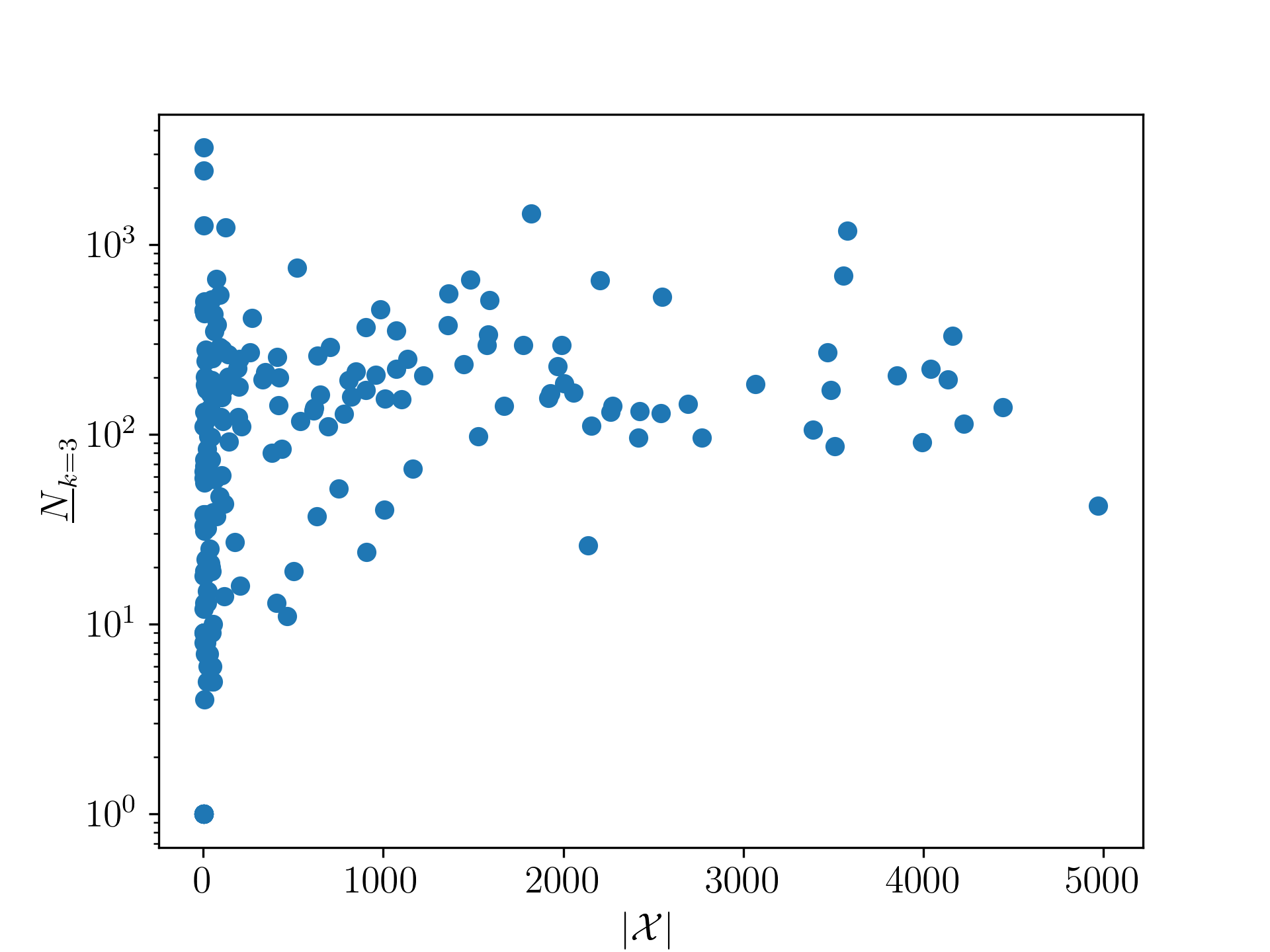
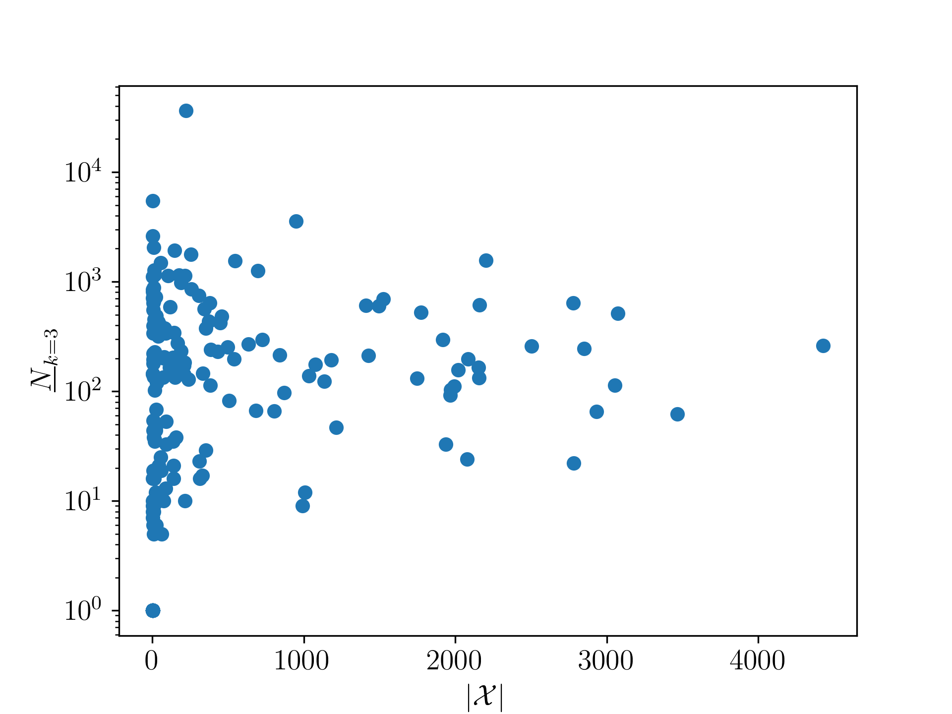
Refer to caption
(a) AL
Refer to caption
(b) NV
Figure 4: There is no clear relationship between $|\mathcal{X}|$ and $\underline{N}_{k}$ for $k=3$.

Figure 2 shows $\underline{N}_{k}$ and $\overline{N}_{k}$ as a function of $m$ for $k=3$. The reduced chain requires orders of magnitude fewer iterations than the simple chain to generate an $\varepsilon$-approximate sample from $\mathcal{X}$. Interestingly, $N_{k}$ appears to be much more consistent as a function of $m$ than $\underline{N}_{\gamma}$ is. Our sample includes two cutoffs (on $m\leq 35$ and $|\mathcal{X}|<5000$), and we might worry that $N_{k}$ will grow dramatically beyond these cutoffs. While we cannot extrapolate beyond them, Figure 2 provides evidence that $N_{k}$ is not growing too quickly near the $m=35$ cutoff. Figure 4 shows that there is no clear relationship between $N_{k}$ and $|\mathcal{X}|$, and some of the largest values of $N_{k}$ come from blocks with small $|\mathcal{X}|$. Again, while we cannot extrapolate beyond the cutoffs in our sample, Figures 2 and 4 do not suggest that $N_{k}$ will be prohibitively large outside of these cutoffs.

Refer to caption
(a) AL
Refer to caption
(b) NV
Figure 5: $k=3$ appears to be optimal because (1) there are blocks for which $M_{k=2}$ is disconnected, and (2) there are blocks for which $M_{k=2}$ is connected by has high mixing time.

Finally, we find that for $k=2$, $M_{k}$ is not irreducible for 2 out of 200 blocks in AL and 3 out of 200 blocks in NV. On the other hand, all blocks in our sample yield irreducible Markov chains for $k\geq 3$. (By construction, if the reduced chain is irreducible for some $k$, it is irreducible for any $k^{\prime}>k$.) Based on these results, $k=3$ appears to be a good choice in this setting. Figure 5 provides a more detailed comparison across $k\in\{2,3,4\}$. Purple plus $\mathord{\text{\char 58}}$ markers denote blocks where the reduced chain is not irreducible for $k=2$. Gold diamond $\blacklozenge$ markers denote blocks for which computation times out (beyond an 8-hour limit) for $k=4$.

Finally, we comment on the computational cost of running the reduced chain in practice. Our results suggest that roughly $10^{5}$ MCMC iterations suffices to generate an $\varepsilon$-approximate sample. In Appendix E, we provide experimental results showing that running this many iterations on a MacBook Pro takes roughly 10 seconds per Census block. Because we process each Census block independently, this can be run efficiently in parallel on a standard computing cluster, requiring tens of days of computing for the states in question (see Appendix E for more details).

4.2.3 Theoretical results for the reduced chain

Here, we provide theoretical results for the reduced chain. In Appendix G, we construct families of pathological instances where where (1) the reduced chain is disconnected for any $k<|\mathcal{X}|$ (Example 2), and (2) the reduced chain is connected for $k=2$ but has exponentially high mixing time (Example 3). Despite this, $M_{k}$ appears to perform quite well for our instances, even though we cannot obtain general subexponential bounds on $N_{k}$ unless P = NP. Here, we attempt to provide intuition for why $M_{k}$ performs well. First, we bound $\log|\mathcal{X}|$. All proofs are deferred to Section D.2.

Lemma 6.

$\log|\mathcal{X}|<\log|\mathcal{Y}|\leq m(1+\log(n+1))$.

Recall that $m$ is the number of households in a Census block. Given that $m$ is reasonably small in our instances (typically on the order of tens, and at most a few thousand), Lemma 6 and 10 imply that $N_{k}$ is primarily determined by the relaxation time $\tau_{\mathrm{rel},k}=1/(1-\lambda_{2}(P_{k}))$.

Corollary 1.

If $\pi(\mathbf{x}_{0})\geq\frac{1}{|\mathcal{X}|}$, then $N_{k}=\tau_{\mathrm{rel},k}\cdot O\left(m\log n\right)$.

We next show conditions under which $M_{k}$ is irreducible.

Lemma 7.

If $\mathcal{V}$ is a hyperrectangle with all interior points, $M_{k}$ is irreducible for $k\geq 2$.

$\mathcal{V}$ is not a hyperrectangle in our setting, so Lemma 7 does not directly apply; however, it offers some insight as to why the reduced chain is irreducible in most of our instances. The set of households is nearly convex, in that given two different households each composed of sets of underlying individuals, it is likely that convex combinations of these households (obtained by “re-shuffling” the underlying individuals) also exist in $\mathcal{V}$. Thus, Lemma 7 provides some intuition that in our fairly “dense” problem setting, we might expect the reduced chain to be irreducible in most cases.

Finally, observe that even when $M_{k}$ is not irreducible, it improves solution quality: a standard coupling argument shows that for any initial distribution $\pi_{0}$, $\|\pi_{0}P_{k}-\pi\|_{1}\leq\|\pi_{0}-\pi\|_{1}$. Moreover, we show that $M_{k}$ converges to a distribution that is in a sense optimal given initial distribution $\pi_{0}$:

Lemma 8.

Let $\{\mathcal{C}_{i}\}_{i=1}^{c}$ be the connected components of the undirected graph induced by $P_{k}$. Given initial state $\mathbb{X}_{0}\sim\pi_{0}$, Algorithm 3 converges to $\pi^{+}(\pi_{0})\triangleq\lim_{t\to\infty}\pi_{0}P_{k}^{t}$ satisfying

$\displaystyle\pi^{+}(\pi_{0})\in\operatorname*{arg\,min}_{\pi^{\prime}:\pi^{\prime}(\mathcal{C}_{i})=\pi_{0}(\mathcal{C}_{i})~{}\forall i\in[c]}d_{\mathrm{TV}}(\pi,\pi^{\prime}).$

In other words, $\pi^{+}(\pi_{0})$ is as close as possible to $\pi$ subject to the constraint that it puts the same probability mass in each connected component that $\pi_{0}$ does.

4.2.4 The reduced chain as a truncation of the simple chain.

We conclude this section with some intuition on the relationship between the simple chain and the reduced chain. We can think of the simple chain as operating on a lattice $\mathcal{L}$ over $\mathbb{Z}_{\geq 0}^{n}$, where each $\mathbf{x}\in\mathcal{Y}$ represents a lattice node. The constraint $\mathbf{V}\mathbf{x}=\mathbf{c}$ is an intersection of hyperplanes $\mathcal{I}$ over $\mathbb{R}^{n}$, and the set of exact solutions $\mathcal{X}$ is the intersection between $\mathcal{L}$ and $\mathcal{I}$. The simple chain corresponds to a random walk over the lattice. The parameter $\gamma$ effectively biases this random walk away from the origin by penalizing nodes exponentially in their distance from $\mathcal{I}$. The reduced chain only operates on $\mathcal{X}=\mathcal{L}\cap\mathcal{I}$. But because transitions are defined by replacing $k$ elements at a time, two states $\mathbf{x},\mathbf{x}^{\prime}\in\mathcal{X}$ have a transition under $P_{k}$ if and only if there is a path between them in $\mathcal{L}$ of length at most $2k$.

This intuition leads to a slightly different way to modify the simple chain: instead of penalizing inexact solutions with $\exp(-\gamma\|\mathbf{V}\mathbf{x}-\mathbf{c}\|_{1})$ as in 5, we could truncate the lattice with a threshold penalty like $\mathbbm{1}[\|\mathbf{V}\mathbf{x}-\mathbf{c}\|_{1}\leq\omega]$ for some parameter $\omega\in\mathbb{Z}_{\geq 0}$. This would prevent the Markov chain from ever transitioning to states that are distance $>\omega$ from $\mathcal{I}$, effectively restricting the state space of the simple chain to be

$\displaystyle\mathcal{Y}_{\omega}\triangleq\{\mathbf{x}:\mathbf{V}\mathbf{x}\preceq\mathbf{c}\wedge\|\mathbf{V}\mathbf{x}-\mathbf{c}\|_{1}\leq\omega\},$

If $\mathcal{X}$ occupies sufficiently large mass within $\mathcal{Y}_{\omega}$, rejection sampling on this chain might lead to a practical algorithm in our setting. Of course, as is the case with the reduced chain, we would no longer be able to guarantee that this modification to the simple chain remains irreducible. We defer such investigations to future work.

5 A Practical Algorithm Based on the Reduced Chain

We conclude with a description of how we implement our algorithm in practice. Because we cannot guarantee that the reduced chain is irreducible, we draw inspiration from Lemma 8 to choose a distribution $\pi_{0}$ over initial states to reduce TVD to the desired distribution even when the reduced chain is not irreducible. Our algorithm has three main hyperparameters: $k$, $t$, and $N$. As before, $k$ gives the number of elements we remove and replace at each iteration of the reduced chain. Larger values of $k$ increase connectivity at the expense of increased computational cost. The number of MCMC iterations we run is $t$, where in our experiments (Section 4.2.2) we found that $t$ on the order of $10^{5}$ seems appropriate.

Finally, $N$ governs our initial state: instead of choosing a single initial state, we use ILP to enumerate the best $N$ solutions according to a linear approximation to $\pi$ (see Section D.1 for details). If a particular block has $|\mathcal{X}_{b}|<N$, we will enumerate all of them, meaning we can simply sample according to $\pi$ with no need for MCMC. If, however, $|\mathcal{X}_{b}|\geq N$, we will enumerate some $\mathcal{S}\subseteq\mathcal{X}$ such that $|\mathcal{S}|=N$. We choose our initial distribution to be $\pi_{0}=(\pi\;|\;\mathbf{x}\in S)$, meaning we sample a random $\mathbf{x}_{0}$ from $\mathcal{S}$ according to $\pi$ and use this as our starting state for MCMC. For a formal description of this algorithm, see Algorithm 4 in Appendix H. This choice of $\pi_{0}$ has two benefits:

  1. 1.

    If $M_{k}$ is not irreducible, the stationary distribution we will converge to is $\pi^{+}(\pi_{0})$ as defined in Lemma 8.

  2. 2.

    If $M_{k}$ is irreducible, this choice of $\pi_{0}$ provides slightly better mixing time guarantees than starting with a single deterministic $\mathbf{x}_{0}$:

Lemma 9.

If $M_{k}$ is irreducible, then Algorithm 4 produces an $\varepsilon$-approximate sample from $\pi$ after at most

$\displaystyle\tau_{\mathrm{mix}}(\varepsilon;P_{k},\mathbb{X})\leq\tau_{\mathrm{rel},k}\log\left(\frac{1}{2\varepsilon\sqrt{\pi(\mathcal{S})}}\right)$

Markov chain iterations.

(Recall that if $|\mathcal{X}_{b}|<N$, then Algorithm 4 does not use MCMC at all.) Thus, the number of MCMC iterations needed reduces as $\mathcal{S}$ captures more probability mass. We prove Lemma 9 in Appendix H.

6 Evaluating and Enforcing Representativeness

Finally, we return to our original goal: generating a dataset such that the marginal distribution over households approximates the PUMS distribution. The PUMS data are very granular, consisting of detailed information on each individual in each household. In contrast, the synthetic microdata are much coarser. Consistent with the SF1 data release, we report the following pieces of information for each household in our microdata:151515We could instead provide more granular information like household status and householder race. This would lead to an increase in total variation distance. We choose to omit them because no downstream analyses we are aware of (including the application of privacy-preserving methods) use these attributes.

  • Number of persons of each of the 7 race categories

  • Number of Hispanic persons

  • Number of adults

Let $\mathcal{H}\subset\mathbb{Z}_{\geq 0}^{9}$ be the set of all possible combinations of household “types” defined this way. Let $h_{i}\in\mathcal{H}$ be the type of household $i\in[n]$. Our goal will be to compare the distribution over types induced by our microdata to the distribution of types found in the PUMS.

To do so, we introduce additional notation. Let $\mathcal{B}$ be the set of blocks in a given state. For a block $b\in\mathcal{B}$, let $\pi_{b}$ be the distribution $\pi$ as defined in 1 for block $b$, let $m_{b}$ be the number of households in block $b$. Then, let $q_{h}$ be the expected frequency of households of type $h$ in our microdata. For $h\in\mathcal{H}$,

$$q_{h}\triangleq\frac{1}{|\mathcal{B}|}\sum_{b\in\mathcal{B}}\frac{1}{m_{b}}\sum_{i:h_{i}=h}\mathbb{E}_{\mathbb{X}\sim\pi_{b}}\left[\mathbb{X}[i]\right].$$ (11)

We can compare this directly with $p_{h}$, defined to be the frequency of households of type $h$ in the PUMS:

$\displaystyle p_{h}\triangleq\sum_{i:h_{i}=h}\Pr_{\mathcal{D}}[\mathbf{v}_{i}].$

Ideally, we would have $q_{h}=p_{h}$ for all $h\in\mathcal{H}$, meaning our methods are unbiased with respect to overall household distribution. However, this will in general not be the case for a variety of reasons. First, as detailed further in Appendix A, data may be incomplete or inconsistent, meaning we cannot always sample from $\mathcal{X}_{b}$ for every block $b$. (In such cases, we coarsen the constraints we enforce to ensure we still get reasonable results.) More subtly, even with perfect data, our induced distribution is not unbiased. Consider the following example with three blocks:

Example 1 (Empirical frequencies may be biased).

Block A contains one household with two white persons (type 1); block B contains two households, each of which contains one white person and one Black person (type 2); and block C contains one household with two Black persons (type 3).

Overall, the frequency of the household types 1, 2, and 3 are $1/4$, $1/2$, and $1/4$ respectively. Given these frequencies, our approach will correctly reconstruct blocks A and C, since there is a unique solution to each of these blocks. Block A can only be reconstructed as a single household of type 1, and block C requires a single household of type 3. However, block B admits multiple possible solutions: it can can be reconstructed either as one household of type 1 and one household of type 3, or as two households of type 2. Under the distribution $\pi$ as defined in 1, these will each be sampled with probabilities 1/3 and 2/3 respectively. As a result, despite the fact that $(p_{1},p_{2},p_{3})=(1/4,1/2,1/4)$, our induced frequencies will be $(q_{1},q_{2},q_{3})=(1/3,1/3,1/3)$. Thus, in general, $q_{h}\neq p_{h}$.

Empirical differences in the household distribution.

Given that our empirical distribution will not be unbiased in general, we empirically evaluate just how close it is. To do so, we use Algorithm 4 to sample a synthetic dataset given by $\{\mathbf{x}_{b}\}_{b\in\mathcal{B}}$ across an entire state. Note that there is an additional source of error here: we do not in general sample from $\pi_{b}$ because when we are unable to completely enumerate $\mathcal{X}_{b}$ (which is precisely when we need the MCMC methods developed earlier) and the reduced chain is not connected, we instead sample from $\pi^{+}(\pi\;|\;\mathbf{x}\in\mathcal{S})$ as defined in Lemma 8.

We will compare the PUMS distribution over types $p_{h}$ to the empirical frequencies $\hat{q}_{h}$ over the household types, defined analogously to 11:

$\displaystyle\hat{q}_{h}\triangleq\frac{1}{|\mathcal{B}|}\sum_{b\in\mathcal{B}}\frac{1}{m_{b}}\sum_{i:h_{i}=h}\mathbf{x}[i].$

In what follows, we only report statistics involving $\hat{q}$ based on a single run of Algorithm 4. Due to the computational cost involved, we are unable to provide confidence intervals. Let $\mathcal{P}$ be the distribution over $\mathcal{H}$ with probabilities given by $p_{h}$, and let $\hat{\mathcal{Q}}$ be the distribution with probabilities $\hat{q}_{h}$. We can now evaluate the distance between our empirical distribution $\mathcal{P}$ and $\hat{\mathcal{Q}}$ using the total variation distance $d_{\mathrm{TV}}(\mathcal{P},\hat{\mathcal{Q}})=\frac{1}{2}\sum_{h\in\mathcal{H}}|p_{h}-\hat{q}_{h}|$.

For Alabama, we find that $d_{\mathrm{TV}}(\mathcal{P},\hat{\mathcal{Q}})=\ALTVDUnadjustedAll$. However, there is a source of error that is beyond our control and, when accounted for, reduces this gap significantly: The PUMS distribution is inconsistent with the distribution reported by SF1. For example, according to SF1, the proportion of single-person households in Alabama is \ALSynSizeOne, whereas according to the PUMS, it is \ALPUMSSizeOne. Because we are constrained to exactly match the number of single-person households reported by SF1, we are guaranteed to incur at least this error relative to the PUMS. To account for this, we re-weight $\mathcal{P}$ to to match the SF1 data on characteristics that are completely determined by SF1, meaning any discrepancy between the PUMS distribution and SF1 are outside our control. Specifically, we re-weight the PUMS distribution to match SF1 on both overall household size (up to size 7) and ethnicity among single-person households (where the proportion of such households is exactly determined by SF1 table P28H), producing $\tilde{\mathcal{P}}$.161616Note that this re-weighting does not affect our original data generation process since the constraints exactly specify the number of households of each size. Under this reweighting, again in Alabama, $d_{\mathrm{TV}}(\tilde{\mathcal{P}},\hat{\mathcal{Q}})=\ALTVDAdjustedAll$. Finally, for data inconsistency or incompleteness reasons detailed in Appendix A, $\mathcal{X}_{b}$ is empty for a some blocks, and we can only solve a coarsened version of our original problem. If we only consider the distribution $\tilde{\mathcal{Q}}$ that excludes these blocks, we find $d_{\mathrm{TV}}(\tilde{\mathcal{P}},\tilde{\mathcal{Q}})=\ALTVDAdjustedAccOne$.

A similar trend holds for NV, summarized in Table 1 (labeled “no reweighting”), though the total variation distance is substantially larger. This is consistent with a broader trend: Nevada requires more MCMC iterations per block, requires MCMC more often (i.e., $|\mathcal{X}_{b}|$ is more often greater than $N$; see Figure 1), and requires more computation time overall relative to Alabama. We speculate that this is because Nevada tends to have more substantially people per block (an average of 75.8, as opposed to 35.3 for Alabama) as well as a larger support for the household distribution $\mathcal{D}$ (i.e., more distinct household types). Replicating our work across more states will likely lead to more insight here.

State $\lambda$ $d_{\mathrm{TV}}(\mathcal{P},\hat{\mathcal{Q}})$ $d_{\mathrm{TV}}(\tilde{\mathcal{P}},\hat{\mathcal{Q}})$ $d_{\mathrm{TV}}(\tilde{\mathcal{P}},\tilde{\mathcal{Q}})$
AL no reweighting \ALTVDUnadjustedAll \ALTVDAdjustedAll \ALTVDAdjustedAccOne
$10^{-3}$ \ALlzzoTVDUnadjustedAll \ALlzzoTVDAdjustedAll \ALlzzoTVDAdjustedAccOne
$10^{-5}$ \ALlzzzzoTVDUnadjustedAll \ALlzzzzoTVDAdjustedAll \ALlzzzzoTVDAdjustedAccOne
NV no reweighting \NVTVDUnadjustedAll \NVTVDAdjustedAll \NVTVDAdjustedAccOne
$10^{-3}$ \NVlzzoTVDUnadjustedAll \NVlzzoTVDAdjustedAll \NVlzzoTVDAdjustedAccOne
$10^{-5}$ \NVlzzzzoTVDUnadjustedAll \NVlzzzzoTVDAdjustedAll \NVlzzzzoTVDAdjustedAccOne
Table 1: Total variation distance between empirical distribution and statewide PUMS.
Improving representativeness via reweighting.

When the PUMS distribution differs substantially from our empirical frequencies, we can adjust the inputs to our algorithm to try to close the gap. Algorithm 4 depends on the input distribution $\mathcal{D}$, and we can reweight $\mathcal{D}$ (drawing some inspiration from Wang et al. (2024)) to produce a new distribution $\mathcal{D}_{\lambda}$ such that, when we run Algorithm 4, the resulting empirical frequencies $\hat{\mathcal{Q}}$ are closer to the original PUMS distribution $\mathcal{P}$. We provide a heuristic in what follows, showing that this reduces total variation distance to $\tilde{\mathcal{P}}$.

Suppose we run Algorithm 4 once, resulting in empirical household type frequencies $\hat{q}_{h}$. Consider the distribution $\mathcal{D}_{\lambda}$ defined as follows for some smoothing parameter $\lambda$:

$\displaystyle\Pr_{\mathcal{D}_{\lambda}}[\mathbf{v}_{i}]\propto\Pr_{\mathcal{D}}[\mathbf{v}_{i}]\cdot\left(\frac{p_{h_{i}}+\lambda}{\hat{q}_{h_{i}}+\lambda}\right).$

We might expect that if we run Algorithm 4 on $\mathcal{D}_{\lambda}$ instead of $\mathcal{D}$, we will end up with a lower total variation distance in our household type distribution. Intuitively, this is because $\mathcal{D}_{\lambda}$ attempts to “correct” for the bias induced by Algorithm 4, boosting the frequency of households that appear infrequently in $\hat{\mathcal{Q}}$ relative to $\mathcal{P}$ and reducing the frequencies of households that are overrepresented. Table 1 shows that reweighting $\mathcal{D}$ decreases total variation distance, though it does not bring it down to 0. It is possible that additional adjustments could reduce TVD further, though it could also be the case that the PUMS distribution is simply incompatible with the constraints from SF1. Reweighting $\mathcal{P}$ to produce $\tilde{\mathcal{P}}$ accounts for this to a limited extent, but there may be no way to satisfy the constraints given by SF1 and simultaneously match the frequencies in the PUMS. This might be an artifact of the PUMS sampling process, since the PUMS is a 10% sample of households taken over several years, or it could be a result of disclosure avoidance steps taken by the Census Bureau before releasing the PUMS data.

Finally, given Example 1, we might wonder whether mixed-race households are likely to be underrepresented in our data. This is indeed the case in both states we analyze, where the frequency of mixed-race households drops from $\ALPUMSMRPct\%$ (AL PUMS) to $\ALSynMRPct\%$ (AL synthetic data) and from $\NVPUMSMRPct\%$ (NV PUMS) to $\NVSynMRPct\%$ (NV synthetic data). At least facially, this can be remedied by artificially boosting the frequencies of mixed-race households in $\mathcal{D}_{\lambda}$. As a crude example, if we let $\lambda=10^{-5}$ and double the frequency of each mixed-race household in $\mathcal{D}_{\lambda}$ (before normalizing it), we raise the frequency of mixed-race households in $\hat{\mathcal{Q}}$ to $\NVmrtwoSynMRPct\%$. Again, further work is needed to determine whether this has broader effects on the realism of the synthetic microdata.

7 Discussion

We have presented algorithms to generate synthetic data and demonstrated that these algorithms are efficient in the Census context. While these data “look like” microdata, it is important to recognize that no sample from this distribution should be treated as ground truth; analyses should look for consistent findings over multiple samples from this distribution. The distribution chosen here is principled, but future work could test whether alternative distributions produce more realistic data, and whether this paradigm of synthetic data generation via combinatorial optimization is appropriate in contexts beyond the Census.

Finally, we comment on potential uses for our synthetic microdata. One clear use case is researchers who seek to study the properties of disclosure avoidance systems. For example, a researcher could generate synthetic data sets, run a disclosure avoidance method on it (e.g., TopDown (Abowd, 2018)), and perform fine-grained analyses of its privacy and accuracy properties. A growing line of work seeks to do just this (e.g., Cohen et al., 2021; Christ et al., 2022; Kenny et al., 2021; Bailie et al., 2023), and the methods presented here will enable a more systematic approach. Moreover, scientists who depend on Census data may be interested in biases induced by disclosure avoidance algorithms (e.g.  Mueller and Santos-Lozada, 2022; Ruggles et al., 2019; Hauer and Santos-Lozada, 2021; Santos-Lozada et al., 2020; Winkler et al., 2021); a potential use for our methods is to estimate and perhaps correct for these biases. If a researcher is interested in a particular statistic measured using Census data, they could estimate the effect that a disclosure avoidance tool will have on that statistic over the distribution of synthetic data we generate. As noted in Section 1, we suggest that all analyses be performed across multiple samples of synthetic data. Used appropriately, the methods presented here can be a valuable tool for researchers to understand the properties of privacy-preserving algorithms.

Future work could extend our methods in a number of different ways. Our particular problem formulation sought to match particular statistics on race, ethnicity, gender, and household size. SF1 data contain far more information than these, however, and in theory one could seek to match other characteristics as well. For instance, researchers interested in studying older populations may wish to match statistics from table P25 (“Households by Presence of People 65 Years and Over, Household Size, and Household Type”). Of course, the more constraints we add, the larger the dimension $d$ of the problem. This could increase the computational cost of finding solutions or overconstrain the problem, making it impossible to solve exactly. A better understanding of this trade-off is needed to take advantage of all of the data provided by SF1. Beyond the Decennial Census, research and public policy often rely on other Census products like the American Community Survey. Extending our methods to these other data releases may be a fruitful avenue for future research. Finally, our formulation treats the state-wide household distribution as invariant conditional on the block-level statistics. If, however, the researcher has more information about geographic variation that the block-level statistics do not encode (for example, that a particular region has more mixed-race households than another), they could in principle encode that information by using a different distribution over households $\mathcal{D}$ for each block.

Ultimately, there is plenty of room to customize the methods we have presented here for any particular use case. Our results have shown that it is possible to efficiently generate samples from a plausible distribution over synthetic Census microdata. Our hope is that researchers will be able to tailor our approach to fit their needs, enabling more comprehensive research into privacy-preserving methods and their broader impacts on downstream analyses.

References

  • Aardal et al. (2000) Karen Aardal, Cor AJ Hurkens, and Arjen K Lenstra. Solving a system of linear Diophantine equations with lower and upper bounds on the variables. Mathematics of operations research, 25(3):427–442, 2000.
  • Abowd (2018) John M Abowd. The US Census Bureau adopts differential privacy. In Proceedings of the 24th ACM SIGKDD international conference on knowledge discovery & data mining, pages 2867–2867, 2018.
  • Abowd (2021) John M. Abowd. Declaration of John Abowd. State of Alabama et al. v. United States Department of Commerce et al., 2021.
  • Abowd et al. (2022) John M Abowd, Robert Ashmead, Ryan Cumings-Menon, Simson Garfinkel, Micah Heineck, Christine Heiss, Robert Johns, Daniel Kifer, Philip Leclerc, Ashwin Machanavajjhala, et al. The 2020 census disclosure avoidance system TopDown algorithm. Harvard Data Science Review, 2, 2022.
  • Achou (1974) O Achou. The number of feasible solutions to a knapsack problem. SIAM Journal on Applied Mathematics, 27(4):606–610, 1974.
  • Bailie et al. (2023) James Bailie, Ruobin Gong, and Xiao-Li Meng. Can swapping be differentially private? A refreshment stirred, not shaken. NBER working paper, 2023.
  • Beged-Dov (1972) Aharon Gavriel Beged-Dov. Lower and upper bounds for the number of lattice points in a simplex. SIAM Journal on Applied Mathematics, 22(1):106–108, 1972.
  • Blankinship (1966) WA Blankinship. Algorithm 288: solution of simultaneous linear Diophantine equations [f4]. Communications of the ACM, 9(7):514, 1966.
  • Bossek et al. (2021) Jakob Bossek, Aneta Neumann, and Frank Neumann. Exact counting and sampling of optima for the knapsack problem. In International Conference on Learning and Intelligent Optimization, pages 40–54. Springer, 2021.
  • Brádler (2016) Kamil Brádler. On the number of nonnegative solutions of a system of linear Diophantine equations. arXiv preprint arXiv:1610.06387, 2016.
  • Bradley (1971) Gordon H Bradley. Algorithms for Hermite and Smith normal matrices and linear Diophantine equations. Mathematics of Computation, 25(116):897–907, 1971.
  • Cabot (1970) A Victor Cabot. An enumeration algorithm for knapsack problems. Operations Research, 18(2):306–311, 1970.
  • Chou and Collins (1982) Tsu-Wu J Chou and George E Collins. Algorithms for the solution of systems of linear Diophantine equations. SIAM Journal on computing, 11(4):687–708, 1982.
  • Christ et al. (2022) Miranda Christ, Sarah Radway, and Steven M Bellovin. Differential privacy and swapping: Examining de-identification’s impact on minority representation and privacy preservation in the US Census. In 2022 IEEE Symposium on Security and Privacy (SP), pages 457–472. IEEE, 2022.
  • Cohen et al. (2021) Aloni Cohen, Moon Duchin, JN Matthews, and Bhushan Suwal. Census TopDown: The impacts of differential privacy on redistricting. In 2nd Symposium on Foundations of Responsible Computing (FORC), 2021.
  • Diaconis and Stroock (1991) Persi Diaconis and Daniel Stroock. Geometric bounds for eigenvalues of Markov chains. The annals of applied probability, pages 36–61, 1991.
  • Dick et al. (2023) Travis Dick, Cynthia Dwork, Michael Kearns, Terrance Liu, Aaron Roth, Giuseppe Vietri, and Zhiwei Steven Wu. Confidence-ranked reconstruction of census microdata from published statistics. Proceedings of the National Academy of Sciences, 120(8):e2218605120, 2023.
  • Dyer (2003) Martin Dyer. Approximate counting by dynamic programming. In Proceedings of the thirty-fifth annual ACM symposium on Theory of computing, pages 693–699, 2003.
  • Dyer et al. (1993) Martin Dyer, Alan Frieze, Ravi Kannan, Ajai Kapoor, Ljubomir Perkovic, and Umesh Vazirani. A mildly exponential time algorithm for approximating the number of solutions to a multidimensional knapsack problem. Combinatorics, Probability and Computing, 2(3):271–284, 1993.
  • Emiris et al. (2017) Ioannis Z Emiris, Anna Karasoulou, and Charilaos Tzovas. Approximating multidimensional subset sum and Minkowski decomposition of polygons. Mathematics in Computer Science, 11:35–48, 2017.
  • Feller (1968) William Feller. An introduction to probability theory and its applications, volume 1. John Wiley & Sons, 3 edition, 1968.
  • Francis (2022) Paul Francis. A note on the misinterpretation of the US Census re-identification attack. In International Conference on Privacy in Statistical Databases, pages 299–311. Springer, 2022.
  • Gawrychowski et al. (2018) Pawel Gawrychowski, Liran Markin, and Oren Weimann. A faster FPTAS for #knapsack. In Ioannis Chatzigiannakis, Christos Kaklamanis, Dániel Marx, and Donald Sannella, editors, 45th International Colloquium on Automata, Languages, and Programming, ICALP, volume 107, pages 64:1–64:13, 2018.
  • Gopalan et al. (2011) Parikshit Gopalan, Adam Klivans, Raghu Meka, Daniel Štefankovic, Santosh Vempala, and Eric Vigoda. An fptas for #knapsack and related counting problems. In 2011 IEEE 52nd Annual Symposium on Foundations of Computer Science, pages 817–826. IEEE, 2011.
  • Guruswami (2016) Venkatesan Guruswami. Rapidly mixing Markov chains: a comparison of techniques (a survey). arXiv preprint arXiv:1603.01512, 2016.
  • Hauer and Santos-Lozada (2021) Mathew E Hauer and Alexis R Santos-Lozada. Differential privacy in the 2020 census will distort COVID-19 rates. Socius, 7:2378023121994014, 2021.
  • Hendrix and Jones (2015) Joe Hendrix and Benjamin F Jones. Bounded integer linear constraint solving via lattice search. In Proceedings of the International Workshop on Satisfiability Modulo Theories, 2015.
  • Hujter (1988) M Hujter. Improved lower and upper bounds for the number of feasible solutions to a knapsack problem. Optimization, 19(6):889–894, 1988.
  • Ingargiola and Korsh (1977) Giorgio P Ingargiola and James F Korsh. A general algorithm for one-dimensional knapsack problems. Operations Research, 25(5):752–759, 1977.
  • Jerrum and Sinclair (1988) Mark Jerrum and Alistair Sinclair. Conductance and the rapid mixing property for Markov chains: the approximation of permanent resolved. In Proceedings of the twentieth annual ACM symposium on Theory of computing, pages 235–244, 1988.
  • Jerrum and Sinclair (1989) Mark Jerrum and Alistair Sinclair. Approximating the permanent. SIAM journal on computing, 18(6):1149–1178, 1989.
  • Jerrum et al. (1986) Mark R Jerrum, Leslie G Valiant, and Vijay V Vazirani. Random generation of combinatorial structures from a uniform distribution. Theoretical computer science, 43:169–188, 1986.
  • Kargin (2011) Vladislav Kargin. Relaxation time is monotone in temperature in the mean-field Ising model. Statistics & probability letters, 81(8):1094–1097, 2011.
  • Kayibi et al. (2018) Koko K Kayibi, Shariefuddin Pirzada, and Carrie Rutherford. Mixing time of Markov chain of the knapsack problem. arXiv preprint arXiv:1803.06914, 2018.
  • Kenny et al. (2021) Christopher T Kenny, Shiro Kuriwaki, Cory McCartan, Evan Rosenman, Tyler Simko, and Kosuke Imai. The use of differential privacy for census data and its impact on redistricting: The case of the 2020 U.S. Census. Science Advances, 7, 2021.
  • Kenny et al. (Forthcoming) Christopher T Kenny, Shiro Kuriwaki, Cory McCartan, Tyler Simko, and Kosuke Imai. Evaluating bias and noise induced by the US Census Bureau’s privacy protection methods. Science Advances, Forthcoming.
  • Kulik and Shachnai (2010) Ariel Kulik and Hadas Shachnai. There is no eptas for two-dimensional knapsack. Information Processing Letters, 110(16):707–710, 2010.
  • Lambe (1974) Thomas A Lambe. Bounds on the number of feasible solutions to a knapsack problem. SIAM Journal on Applied Mathematics, 26(2):302–305, 1974.
  • Lambe (1977) Thomas A Lambe. Upper bound on the number of nonnegative integer solutions to a linear equation. SIAM Journal on Applied Mathematics, 32(1):215–219, 1977.
  • Lawler (1979) Eugene L Lawler. Fast approximation algorithms for knapsack problems. Mathematics of Operations Research, 4:339–356, 1979.
  • Lawler and Sokal (1988) Gregory F Lawler and Alan D Sokal. Bounds on the $L^{2}$ spectrum for Markov chains and Markov processes: a generalization of Cheeger’s inequality. Transactions of the American mathematical society, 309(2):557–580, 1988.
  • Lazebnik (1996) Felix Lazebnik. On systems of linear Diophantine equations. Mathematics Magazine, 69(4):261–266, 1996.
  • Levin et al. (2017) David A Levin, Yuval Peres, and Elizabeth L Wilmer. Markov chains and mixing times. American Mathematical Soc., 2017.
  • Magazine and Chern (1984) Michael J Magazine and Maw-Sheng Chern. A note on approximation schemes for multidimensional knapsack problems. Mathematics of Operations Research, 9(2):244–247, 1984.
  • Mahmoudvand et al. (2010) Rahim Mahmoudvand, Hossein Hassani, Abbas Farzaneh, and Gareth Howell. The exact number of nonnegative integer solutions for a linear Diophantine inequality. IAENG International Journal of Applied Mathematics, 40(1):1–5, 2010.
  • Martello and Toth (1987) Silvano Martello and Paolo Toth. Algorithms for knapsack problems. North-Holland Mathematics Studies, 132:213–257, 1987.
  • Morris and Sinclair (2004) Ben Morris and Alistair Sinclair. Random walks on truncated cubes and sampling 0-1 knapsack solutions. SIAM journal on computing, 34(1):195–226, 2004.
  • Mueller and Santos-Lozada (2022) J Tom Mueller and Alexis R Santos-Lozada. The 2020 US Census differential privacy method introduces disproportionate discrepancies for rural and non-white populations. Population Research and Policy Review, 41(4):1417–1430, 2022.
  • Nacu (2003) Şerban Nacu. Glauber dynamics on the cycle is monotone. Probability theory and related fields, 127:177–185, 2003.
  • OEIS Foundation Inc. (2023) OEIS Foundation Inc. The On-Line Encyclopedia of Integer Sequences, 2023. Published electronically at http://oeis.org.
  • Padberg (1971) Manfred W Padberg. A remark on “An inequality for the number of lattice points in a simplex”. SIAM Journal on Applied Mathematics, 20(4):638–641, 1971.
  • Petti and Flaxman (2019) Samantha Petti and Abraham Flaxman. Differential privacy in the 2020 US census: What will it do? Quantifying the accuracy/privacy tradeoff. Gates open research, 3, 2019.
  • Pisinger (1999) David Pisinger. An exact algorithm for large multiple knapsack problems. European Journal of Operational Research, 114(3):528–541, 1999.
  • Porod (2024) Ursula Porod. Dynamics of Markov Chains for Undergraduates. Preprint, 2024. URL https://www.math.northwestern.edu/documents/book-markov-chains.pdf.
  • Puchinger et al. (2010) Jakob Puchinger, Günther R Raidl, and Ulrich Pferschy. The multidimensional knapsack problem: Structure and algorithms. INFORMS Journal on Computing, 22(2):250–265, 2010.
  • Rizzi and Tomescu (2014) Romeo Rizzi and Alexandru I Tomescu. Faster fptases for counting and random generation of knapsack solutions. In European Symposium on Algorithms, pages 762–773. Springer, 2014.
  • Ruggles et al. (2019) Steven Ruggles, Catherine Fitch, Diana Magnuson, and Jonathan Schroeder. Differential privacy and census data: Implications for social and economic research. In AEA papers and proceedings, volume 109, pages 403–408. American Economic Association 2014 Broadway, Suite 305, Nashville, TN 37203, 2019.
  • Ruggles et al. (2024) Steven Ruggles, Sarah Flood, Matthew Sobek, Daniel Backman, Annie Chen, Grace Cooper, Stephanie Richards, Renae Rodgers, and Megan Schouweiler. IPUMS USA: Version 15.0 [dataset], 2024.
  • Salkin and De Kluyver (1975) Harvey M Salkin and Cornelis A De Kluyver. The knapsack problem: a survey. Naval Research Logistics Quarterly, 22(1):127–144, 1975.
  • Sánchez-Roselly Navarro (2016) Alfredo Sánchez-Roselly Navarro. Linear Diophantine equations and applications. PhD thesis, Universidad de Granada, 2016.
  • Santos-Lozada et al. (2020) Alexis R Santos-Lozada, Jeffrey T Howard, and Ashton M Verdery. How differential privacy will affect our understanding of health disparities in the United States. Proceedings of the National Academy of Sciences, 117(24):13405–13412, 2020.
  • Sinclair and Jerrum (1989) Alistair Sinclair and Mark Jerrum. Approximate counting, uniform generation and rapidly mixing markov chains. Information and Computation, 82(1):93–133, 1989.
  • Sousi (2020) Perla Sousi. Mixing times of Markov chains. Preprint, 2020. URL https://personal.math.ubc.ca/~jhermon/Mixing/mixing-notes.pdf.
  • Stanley (1999) Richard P Stanley. Enumerative combinatorics, volume 2. Cambridge university press, 1999.
  • Steed et al. (2022) Ryan Steed, Terrance Liu, Zhiwei Steven Wu, and Alessandro Acquisti. Policy impacts of statistical uncertainty and privacy. Science, 377(6609):928–931, 2022.
  • Wang et al. (2024) Hao Wang, Shivchander Sudalairaj, John Henning, Kristjan Greenewald, and Akash Srivastava. Post-processing private synthetic data for improving utility on selected measures. Advances in Neural Information Processing Systems, 36, 2024.
  • Winkler et al. (2021) Richelle L Winkler, Jaclyn L Butler, Katherine J Curtis, and David Egan-Robertson. Differential privacy and the accuracy of county-level net migration estimates. Population Research and Policy Review, pages 1–19, 2021.
Organization of the appendix.

Appendix A contains detailed information on our encoding of Census data into $d$-dimensional vectors. We present a rejection sampling algorithm that is equivalent to our algorithm under our choice of $\pi$ in Appendix B. In Appendices C and D, we provide omitted proofs and details from Sections 4.1 and 4.2 respectively. We present additional empirical results for both the simple and reduced chains in Appendix E. We formally show that MMS is NP-hard in Appendix F. In Appendix G, we construct pathological synthetic examples under which the reduced chain is either not irreducible or has exponentially large mixing time. Finally, in Appendix H, we describe our final algorithm and theoretically characterize its performance.

Appendix A Data Encoding Details

Census data is encoded with 7 race categories (white, Black, American Indian and Native Alaskan, Asian, Hawaiian and Pacific Islander, other, and two or more) and two ethnicity categories (Hispanic or non-Hispanic). We encode each distinct household $\mathbf{v}_{i}$ and block-level statistic $\mathbf{c}$ as a 135-dimensional integer vector. The encoding is as follows, annotated with the dimensionality of each component:

  • Number of individuals of each (race, ethnicity) combination (14)

  • Number of adults (defined as 18 or older) of each race (7)

  • Number of Hispanic adults (1)

  • (Householder race) $\times$ (whether or not the household is a family) $\times$ (household size in $\{1,2,3,4,5,6,7+\}$) (98). Note that these form a partition, so every household has a 1 in exactly one of these 98 components.

  • For households with Hispanic householders, (whether or not the household is a family) $\times$ (household size in $\{1,2,3,4,5,6,7+\}$) (14)171717Because ethnicity is encoded as a binary variable and the remaining two attributes are completely determined by the (race) $\times$ (is family) $\times$ (household size) variables, including both (Householder is Hispanic) and (Householder is not Hispanic) is redundant here.

  • Number of households (a constant 1 for each household) (1)

Each row of the PUMS sample contains all of this information. We choose this particular encoding because this information can also be found in block-level aggregate data from SF1.181818SF1 data can be accessed at https://www.nhgis.org/. Each block-level vector $\mathbf{c}$ is the sum of the these characteristics of all households in the block. These totals can be found in a combination of SF1 tables P3, P28AH, and P16AH. These data are not always internally consistent: tables that purport to represent the same information (e.g., the number of adults living in a block) disagree for a small fraction of blocks (around 1% in both AL and NV). We exclude these blocks from our analysis. Moreover, there are blocks for which no solution to our optimization problem exists (i.e., no combination of PUMS households matches the reported block totals). This can happen because the PUMS data are incomplete, since a “rare” household might be needed to match the block-level constraints. We exclude these blocks as well (about 5% in AL and 14% in NV). In our publicly available code, when we encounter such blocks, we simply reduce the dimensionality of the vectors and apply the same techniques to solve them. For example, instead of matching the number of adults of each race and ethnicity, we simply match the total number of adults in the block.

There are $n=2,745$ distinct households (encoded as 135-dimensional vectors) in the AL PUMS and $n=4,094$ distinct households in the NV PUMS. The data we use are subject to disclosure avoidance systems before their release. They do not represent “ground truth”; nevertheless, we treat them as the source of the distribution we seek to sample from. Downstream analyses should be careful not to rely on the exact locations of very rare households, since these are unlikely to be accurate.

Appendix B Rejection Sampling Formulation

Here, we present a rejection sampling algorithm (Algorithm 1) that samples from $\mathcal{X}$ according to the distribution given in 1. This algorithm is far too inefficient to be practical; it is intended simply to illustrate and provide motivation for the problem specification here.

Algorithm 1 RejectionSampling$(\mathbf{V},\mathbf{c},\mathcal{D})$
repeat$\triangleright$ Repeat until a sample is accepted
     $\mathbf{x}\leftarrow\mathbf{0}\in\mathbb{Z}_{\geq 0}^{n}$ $\triangleright$ Empty multiset
     while $\mathbf{V}\mathbf{x}\preceq\mathbf{c}$ do $\triangleright$ $\preceq$ denotes element-wise $\leq$.
         Sample $\mathbf{v}_{i}$ from $\mathcal{D}$
         $\mathbf{x}[i]\leftarrow\mathbf{x}[i]+1$
     end while
until $\mathbf{V}\mathbf{x}=\mathbf{c}$
return 𝐱𝐱\mathbf{x}

Appendix C Omitted Proofs and Details from Section 4.1

C.1 Formal algorithm description for the simple chain

Algorithm 2 Simple($\mathbf{V},\mathbf{c},f,\gamma,t$)
repeat
     $\mathbf{x}\leftarrow\mathbf{0}\in\mathbb{Z}_{\geq 0}^{n}$
     for t𝑡t iterations do
         with probability 0.50.50.5
              continue
         end
         $i\leftarrow$ a random integer in $[n]$ such that $\mathbf{v}_{i}\preceq\mathbf{c}$ $\triangleright$ Ignore ineligible households
         $\mathbf{r}\leftarrow\mathbf{c}-\mathbf{V}\mathbf{x}_{i\leftarrow 0}$
         $g_{\max}\leftarrow\max~{}\{g\in\mathbb{Z}_{\geq 0}:g\mathbf{v}_{i}\preceq\mathbf{r}\}$
         $\mathcal{S}\leftarrow\{\mathbf{x}_{i\leftarrow g}:0\leq g\leq g_{\max}\}$
         $\mathbf{x}\leftarrow$ a random sample from $\tilde{\pi}_{\gamma}\;|\;\mathbf{x}\in\mathcal{S}$ (i.e., $\propto f(\mathbf{x})\exp(-\gamma\|\mathbf{V}\mathbf{x}-\mathbf{c}\|)$ on $\mathcal{S}$)
     end for
until $\mathbf{V}\mathbf{x}=\mathbf{c}$
return 𝐱𝐱\mathbf{x}

C.2 Theoretical results for the simple chain

First, we prove Lemma 2. We restate each result before proving it. See 2

Proof.

First, we show that bounded TVD implies bounded TVD on conditional distributions, inflated by a factor of $1/\sigma(\mathcal{X})$.

$\displaystyle d_{\mathrm{TV}}(\sigma,\sigma^{\prime})$ $\displaystyle\leq\varepsilon$
$\displaystyle\|\sigma-\sigma^{\prime}\|_{1}$ $\displaystyle\leq 2\varepsilon$
$\displaystyle\sum_{\mathbf{x}\in\mathcal{X}}|\sigma(\mathbf{x})-\sigma^{\prime}(\mathbf{x})|$ $\displaystyle\leq 2\varepsilon$
$\displaystyle\sum_{\mathbf{x}\in\mathcal{X}}\left|\frac{\sigma(\mathbf{x})}{\sigma(\mathcal{X})}-\frac{\sigma^{\prime}(\mathbf{x})}{\sigma(\mathcal{X})}\right|$ $\displaystyle\leq\frac{2\varepsilon}{\sigma(\mathcal{X})}$
$\displaystyle\sum_{\mathbf{x}\in\mathcal{X}}\left|\frac{\sigma(\mathbf{x})}{\sigma(\mathcal{X})}-\frac{\sigma^{\prime}(\mathbf{x})}{\sigma^{\prime}(\mathcal{X})}+\frac{\sigma^{\prime}(\mathbf{x})}{\sigma^{\prime}(\mathcal{X})}-\frac{\sigma^{\prime}(\mathbf{x})}{\sigma(\mathcal{X})}\right|$ $\displaystyle\leq\frac{2\varepsilon}{\sigma(\mathcal{X})}$
$\displaystyle\sum_{\mathbf{x}\in\mathcal{X}}\left|\frac{\sigma(\mathbf{x})}{\sigma(\mathcal{X})}-\frac{\sigma^{\prime}(\mathbf{x})}{\sigma^{\prime}(\mathcal{X})}\right|-\left|\frac{\sigma^{\prime}(\mathbf{x})}{\sigma^{\prime}(\mathcal{X})}-\frac{\sigma^{\prime}(\mathbf{x})}{\sigma(\mathcal{X})}\right|$ $\displaystyle\leq\frac{2\varepsilon}{\sigma(\mathcal{X})}$ (triangle inequality)
$\displaystyle\sum_{\mathbf{x}\in\mathcal{X}}\left|\sigma_{\mathcal{X}}(\mathbf{x})-\sigma_{\mathcal{X}}^{\prime}(\mathbf{x})\right|-\sigma^{\prime}(\mathbf{x})\left|\frac{1}{\sigma^{\prime}(\mathcal{X})}-\frac{1}{\sigma(\mathcal{X})}\right|$ $\displaystyle\leq\frac{2\varepsilon}{\sigma(\mathcal{X})}$
$\displaystyle\|\sigma_{\mathcal{X}}-\sigma_{\mathcal{X}}^{\prime}\|_{1}-\sigma^{\prime}(\mathcal{X})\left|\frac{1}{\sigma^{\prime}(\mathcal{X})}-\frac{1}{\sigma(\mathcal{X})}\right|$ $\displaystyle\leq\frac{2\varepsilon}{\sigma(\mathcal{X})}$
$\displaystyle\|\sigma_{\mathcal{X}}-\sigma_{\mathcal{X}}^{\prime}\|_{1}$ $\displaystyle\leq\frac{2\varepsilon}{\sigma(\mathcal{X})}+\sigma^{\prime}(\mathcal{X})\frac{|\sigma(\mathcal{X})-\sigma^{\prime}(\mathcal{X})|}{\sigma^{\prime}(\mathcal{X})\sigma(\mathcal{X})}$
$\displaystyle\|\sigma_{\mathcal{X}}-\sigma_{\mathcal{X}}^{\prime}\|_{1}$ $\displaystyle\leq\frac{2\varepsilon}{\sigma(\mathcal{X})}+\frac{|\sigma(\mathcal{X})-\sigma^{\prime}(\mathcal{X})|}{\sigma(\mathcal{X})}$
$\displaystyle\|\sigma_{\mathcal{X}}-\sigma_{\mathcal{X}}^{\prime}\|_{1}$ $\displaystyle\leq\frac{3\varepsilon}{\sigma(\mathcal{X})}$ ($d_{\mathrm{TV}}(\sigma,\sigma^{\prime})\leq\varepsilon$)
$\displaystyle d_{\mathrm{TV}}(\sigma_{\mathcal{X}},\sigma_{\mathcal{X}}^{\prime})$ $\displaystyle\leq\frac{3\varepsilon}{2\sigma(\mathcal{X})}$

To show that this is tight to within a constant factor, consider an instance where $\mathcal{X}=\{\mathbf{x}_{0},\mathbf{x}_{1}\}$ and assume without loss of generality $\sigma(\mathbf{x}_{0})\leq\sigma(\mathbf{x}_{1})$. For a given $\varepsilon$ define $\sigma^{\prime}$ as follows:

$\displaystyle\sigma^{\prime}(\mathbf{x}_{0})$ $\displaystyle=\sigma(\mathbf{x}_{0})+\varepsilon$
$\displaystyle\sigma^{\prime}(\mathbf{x}_{1})$ $\displaystyle=\max(0,\sigma(\mathbf{x}_{1})-\varepsilon)$
$\displaystyle\sigma^{\prime}(\mathbf{x})$ $\displaystyle=\begin{cases}\sigma(\mathbf{x})&\sigma(\mathbf{x}_{1})\geq\varepsilon\\ \sigma(\mathbf{x})\left(1-\frac{\varepsilon-\sigma(\mathbf{x}_{1}))}{1-\sigma(\mathcal{X})}\right)&\sigma(\mathbf{x}_{1})<\varepsilon\end{cases}$ ($\mathbf{x}\notin\mathcal{X}$)

First, observe that if $\sigma(\mathbf{x}_{1})<\varepsilon$, then $\sigma^{\prime}(\mathbf{x}_{1})=0$ and $d_{\mathrm{TV}}(\sigma_{\mathcal{X}},\sigma^{\prime}_{\mathcal{X}})\geq\frac{1}{2}$. This is within a factor of 2 of our upper bound since trivially $d_{\mathrm{TV}}(\sigma_{\mathcal{X}},\sigma^{\prime}_{\mathcal{X}})\leq 1$. If $\sigma(\mathbf{x}_{1})\geq\varepsilon$, then

$\displaystyle d_{\mathrm{TV}}(\sigma_{\mathcal{X}},\sigma^{\prime}_{\mathcal{X}})$ $\displaystyle=\frac{1}{2}\|\sigma_{\mathcal{X}}-\sigma^{\prime}_{\mathcal{X}}\|_{1}$
$\displaystyle=\frac{1}{2}\sum_{\mathbf{x}\in\mathcal{X}}|\sigma_{\mathcal{X}}(\mathbf{x})-\sigma^{\prime}_{\mathcal{X}}(\mathbf{x})|$
$\displaystyle=\frac{1}{2}\sum_{\mathbf{x}\in\mathcal{X}}\left|\frac{\sigma(\mathbf{x})}{\sigma(\mathcal{X})}-\frac{\sigma^{\prime}(\mathbf{x})}{\sigma^{\prime}(\mathcal{X})}\right|$
$\displaystyle=\frac{1}{2}\sum_{\mathbf{x}\in\mathcal{X}}\left|\frac{\sigma(\mathbf{x})}{\sigma(\mathcal{X})}-\frac{\sigma^{\prime}(\mathbf{x})}{\sigma(\mathcal{X})}\right|$ ($\sigma^{\prime}(\mathcal{X})=\sigma(\mathcal{X})$)
$\displaystyle=\frac{1}{2\sigma(\mathcal{X})}\sum_{\mathbf{x}\in\mathcal{X}}\left|\sigma(\mathbf{x})-\sigma^{\prime}(\mathbf{x})\right|$
$\displaystyle=\frac{1}{2\sigma(\mathcal{X})}(|\sigma(\mathbf{x}_{0})-\sigma^{\prime}(\mathbf{x}_{0})|+|\sigma(\mathbf{x}_{1})-\sigma^{\prime}(\mathbf{x}_{1})|)$
$\displaystyle=\frac{\varepsilon}{\sigma(\mathcal{X})}$

We next provide a theoretical explanation for the poor performance of the simple chain here, which we will use to motivate the reduced chain in Section 4.2. In particular, we characterize how $\gamma$ impacts $N_{\gamma}$. We show how varying $\gamma$ creates a trade-off between raising $p_{\gamma}^{*}$ and lowering $t^{*}_{\gamma}(\varepsilon)$. First, we show that $p_{\gamma}^{*}$ increases with $\gamma$, ranging from 0 to 1 as $\gamma$ ranges from $-\infty$ to $\infty$.

See 3

Proof.

First, we show that $p_{\gamma}^{*}$ is monotonically increasing in $\gamma$. By definition,

$\displaystyle\frac{d}{d\gamma}p_{\gamma}^{*}$ $\displaystyle=\frac{d}{d\gamma}\frac{\tilde{\pi}_{\gamma}(\mathcal{X})}{\tilde{\pi}_{\gamma}(\mathcal{Y})}$
$\displaystyle=\frac{\tilde{\pi}_{\gamma}(\mathcal{Y})\frac{d}{d\gamma}\tilde{\pi}_{\gamma}(\mathcal{X})-\tilde{\pi}_{\gamma}(\mathcal{X})\frac{d}{d\gamma}\tilde{\pi}_{\gamma}(\mathcal{Y})}{\tilde{\pi}_{\gamma}(\mathcal{Y})^{2}}$
$\displaystyle=\frac{-\tilde{\pi}_{\gamma}(\mathcal{X})\frac{d}{d\gamma}\tilde{\pi}_{\gamma}(\mathcal{Y})}{\tilde{\pi}_{\gamma}(\mathcal{Y})^{2}}.$

Because $\tilde{\pi}_{\gamma}(\cdot)>0$, it suffices to show

$\displaystyle\frac{d}{d\gamma}\tilde{\pi}_{\gamma}(\mathcal{Y})$ $\displaystyle=\frac{d}{d\gamma}\sum_{\mathbf{x}^{\prime}\in\mathcal{Y}}\tilde{\pi}_{\gamma}(\mathbf{x}^{\prime})$
$\displaystyle=\sum_{\mathbf{x}^{\prime}\in\mathcal{Y}}\frac{d}{d\gamma}\exp(-\gamma\|\mathbf{c}-\mathbf{V}\mathbf{x}^{\prime}\|_{1})f(\mathbf{x}^{\prime})$
$\displaystyle=\sum_{\mathbf{x}^{\prime}\in\mathcal{Y}}-\|\mathbf{c}-\mathbf{V}\mathbf{x}^{\prime}\|_{1}\exp(-\gamma\|\mathbf{c}-\mathbf{V}\mathbf{x}^{\prime}\|_{1})f(\mathbf{x}^{\prime})$
$\displaystyle<0.$

Next, we show that $p_{\gamma}^{*}$ has the claimed limits. Note that ignoring the normalizing constant, $\gamma$ has no effect on $\tilde{\pi}_{\gamma}(\mathbf{x})$ for any $\mathbf{x}\in\mathcal{X}$, since $\|\mathbf{c}-\mathbf{V}\mathbf{x}\|_{1}=0$ for any such $\mathbf{x}$. On the other hand, for any $\mathbf{x}^{\prime}\in\mathcal{Y}\backslash\mathcal{X}$ and $\gamma<0$,

$\displaystyle\tilde{\pi}_{\gamma}(\mathbf{x}^{\prime})\propto\exp(-\gamma\|\mathbf{c}-\mathbf{V}\mathbf{x}^{\prime}\|_{1})f(\mathbf{x}^{\prime})\geq\exp(-\gamma)f(\mathbf{x}^{\prime})$

Therefore,

$\displaystyle\lim_{\gamma\to-\infty}p_{\gamma}^{*}$ $\displaystyle=\lim_{\gamma\to-\infty}\frac{\tilde{\pi}_{\gamma}(\mathcal{X})}{\tilde{\pi}_{\gamma}(\mathcal{Y})}$
$\displaystyle\leq\lim_{\gamma\to-\infty}\frac{\tilde{\pi}_{\gamma}(\mathcal{X})}{\tilde{\pi}_{\gamma}(\mathcal{Y}\backslash\mathcal{X})}$
$\displaystyle=\lim_{\gamma\to-\infty}\frac{\sum_{\mathbf{x}\in\mathcal{X}}\tilde{\pi}_{\gamma}(\mathbf{x})}{\sum_{\mathbf{x}^{\prime}\in\mathcal{Y}\backslash\mathcal{X}}\tilde{\pi}_{\gamma}(\mathbf{x}^{\prime})}$
$\displaystyle\leq\lim_{\gamma\to-\infty}\frac{\sum_{\mathbf{x}\in\mathcal{X}}f(\mathbf{x})}{\exp(-\gamma)\sum_{\mathbf{x}^{\prime}\in\mathcal{Y}\backslash\mathcal{X}}f(\mathbf{x}^{\prime})}$
$\displaystyle=0$

Similarly, for $\mathbf{x}^{\prime}\in\mathcal{Y}\backslash\mathcal{X}$ and $\gamma>0$,

$\displaystyle\tilde{\pi}_{\gamma}(\mathbf{x}^{\prime})=\exp(\gamma\|\mathbf{c}-\mathbf{V}\mathbf{x}^{\prime}\|_{1})f(\mathbf{x}^{\prime})\leq\exp(\gamma)f(\mathbf{x}^{\prime})$

Therefore,

$\displaystyle\lim_{\gamma\to\infty}p_{\gamma}^{*}$ $\displaystyle=\lim_{\gamma\to\infty}\frac{\tilde{\pi}_{\gamma}(\mathcal{X})}{\tilde{\pi}_{\gamma}(\mathcal{Y})}$
$\displaystyle=\lim_{\gamma\to\infty}\frac{\tilde{\pi}_{\gamma}(\mathcal{X})}{\tilde{\pi}_{\gamma}(\mathcal{Y}\backslash\mathcal{X})+\tilde{\pi}_{\gamma}(\mathcal{X})}$
$\displaystyle=\lim_{\gamma\to\infty}\frac{\tilde{\pi}_{\gamma}(\mathcal{X})}{\sum_{\mathbf{x}^{\prime}\in\mathcal{Y}\backslash\mathcal{X}}\tilde{\pi}_{\gamma}(\mathbf{x}^{\prime})+\tilde{\pi}_{\gamma}(\mathcal{X})}$
$\displaystyle\geq\lim_{\gamma\to\infty}\frac{\tilde{\pi}_{\gamma}(\mathcal{X})}{\exp(-\gamma)\sum_{\mathbf{x}^{\prime}\in\mathcal{Y}\backslash\mathcal{X}}f(\mathbf{x}^{\prime})+\tilde{\pi}_{\gamma}(\mathcal{X})}$
$\displaystyle=1$

See 4

Proof.

We will provide a lower an upper bound on the conductance of $M_{\gamma}$ and use Cheeger’s inequality to lower-bound the mixing time. The conductance (see, e.g., Guruswami, 2016) of $M_{\gamma}$ is defined as

$$\Phi(M_{\gamma})=\min_{\begin{subarray}{c}\mathcal{S}\subset\mathcal{Y}\\ 0<\tilde{\pi}_{\gamma}(\mathcal{S})\leq 1/2\end{subarray}}\frac{Q_{\gamma}(\mathcal{S},\overline{\mathcal{S}})}{\tilde{\pi}_{\gamma}(\mathcal{S})}$$ (12)

where $Q_{\gamma}(\mathbf{x},\mathbf{x}^{\prime})=\tilde{\pi}_{\gamma}(\mathbf{x})P_{\gamma}(\mathbf{x},\mathbf{x}^{\prime})$ and $Q_{\gamma}(\mathcal{S},\overline{\mathcal{S}})=\sum_{\mathbf{x}\in\mathcal{S},\mathbf{x}^{\prime}\notin\mathcal{S}}Q_{\gamma}(\mathbf{x},\mathbf{x}^{\prime})$. We will show that in particular, $Q_{\gamma}(\mathcal{X},\overline{\mathcal{X}})/\tilde{\pi}_{\gamma}(\mathcal{X})$ is small, providing an upper bound for $\Phi(M_{\gamma})$.

To do so, let $p_{i}=\Pr_{\mathcal{D}}[\mathbf{v}_{i}]$ and $\ell$ = $\|\mathbf{v}_{i}\|_{1}$. Observe that for any $\mathbf{x}\in\mathcal{X}$ and $i\in[n]$, if $\gamma$ is sufficiently large,

$\displaystyle\frac{\tilde{\pi}_{\gamma}(\mathbf{x})}{\tilde{\pi}_{\gamma}(\Delta(\mathbf{x},i))}$ $\displaystyle=\frac{\tilde{\pi}_{\gamma}(\mathbf{x})}{\sum_{g=0}^{\mathbf{x}[i]}\tilde{\pi}_{\gamma}(\mathbf{x}_{i\leftarrow g})}$
$\displaystyle=\frac{f(\mathbf{x})}{\sum_{g=0}^{\mathbf{x}[i]}f(\mathbf{x}_{i\leftarrow g})\exp(-\gamma\|\mathbf{c}-\mathbf{V}\mathbf{x}_{i\leftarrow g}\|_{1})}$
$\displaystyle=\frac{f(\mathbf{x})}{\sum_{g=0}^{\mathbf{x}[i]}f(\mathbf{x}_{i\leftarrow(\mathbf{x}[i]-g)})\exp(-\gamma\|\mathbf{c}-\mathbf{V}\mathbf{x}_{i\leftarrow(\mathbf{x}[i]-g)}\|_{1})}$
$\displaystyle=\frac{f(\mathbf{x})}{\sum_{g=0}^{\mathbf{x}[i]}f(\mathbf{x}_{i\leftarrow(\mathbf{x}[i]-g)})\exp(-\gamma g\|\mathbf{v}_{i}\|_{1})}$
$\displaystyle=\frac{1}{1+\sum_{g=1}^{\mathbf{x}[i]}\frac{f(\mathbf{x}_{i\leftarrow(\mathbf{x}[i]-g)})}{f(\mathbf{x})}\exp(-\gamma g\ell)}$
$\displaystyle\geq 1-\sum_{g=1}^{\mathbf{x}[i]}\frac{f(\mathbf{x}_{i\leftarrow(\mathbf{x}[i]-g)})}{f(\mathbf{x})}\exp(-\gamma g\ell)$ ($\frac{1}{1+a}\geq 1-a$ for $a\geq 0$)
$\displaystyle=1-\sum_{g=1}^{\mathbf{x}[i]}\frac{\binom{k-g}{\mathbf{x}[i]-g}}{\binom{k}{\mathbf{x}[i]}p_{i}^{g}}\exp(-\gamma g\ell)$
$\displaystyle\geq 1-\sum_{g=1}^{\mathbf{x}[i]}p_{i}^{-g}\exp(-\gamma g\ell)$
$\displaystyle=1-\sum_{g=1}^{\mathbf{x}[i]}(p_{i}\exp(\gamma\ell))^{-g}$
$\displaystyle\geq 1-\sum_{g=1}^{\infty}(p_{i}\exp(\gamma\ell))^{-g}$
$\displaystyle=1-\frac{p_{i}^{-1}\exp(-\gamma\ell)}{1-p_{i}^{-1}\exp(-\gamma\ell)}$ (for $p_{i}^{-1}\exp(-\gamma\ell)<1$)
$\displaystyle\geq 1-2(\min_{i}p_{i})^{-1}\exp(-\gamma\ell)$ (for $p_{i}^{-1}\exp(-\gamma\ell)<1/2$)
$\displaystyle=1-R\exp(-\gamma\ell)$ (13)

for $R\triangleq 2(\min_{i}p_{i})^{-1}$. With this,

$\displaystyle\frac{Q_{\gamma}(\mathcal{X},\overline{\mathcal{X}})}{\tilde{\pi}_{\gamma}(\mathcal{X})}$ $\displaystyle=\frac{\sum_{\mathbf{x}\in\mathcal{X},\mathbf{x}^{\prime}\in\overline{\mathcal{X}}_{\mathbf{x}}}\tilde{\pi}_{\gamma}(\mathbf{x})P_{\gamma}(\mathbf{x},\mathbf{x}^{\prime})}{\tilde{\pi}_{\gamma}(\mathcal{X})}$
$\displaystyle=\frac{\sum_{\mathbf{x}\in\mathcal{X}}\tilde{\pi}_{\gamma}(\mathbf{x})\sum_{\mathbf{x}^{\prime}\in\overline{\mathcal{X}}_{\mathbf{x}}}P_{\gamma}(\mathbf{x},\mathbf{x}^{\prime})}{\tilde{\pi}_{\gamma}(\mathcal{X})}$
$\displaystyle=\frac{\sum_{\mathbf{x}\in\mathcal{X}}\tilde{\pi}_{\gamma}(\mathbf{x})\sum_{i\in[n]}\sum_{\mathbf{x}^{\prime}\in\overline{\mathcal{X}}_{\mathbf{x}}\cap\Delta(\mathbf{x},i)}\frac{\tilde{\pi}_{\gamma}(\mathbf{x}^{\prime})}{2n\tilde{\pi}_{\gamma}(\Delta(\mathbf{x},i))}}{\tilde{\pi}_{\gamma}(\mathcal{X})}$
$\displaystyle=\frac{\sum_{\mathbf{x}\in\mathcal{X}}\tilde{\pi}_{\gamma}(\mathbf{x})\sum_{i\in[n]}\frac{\tilde{\pi}_{\gamma}(\Delta(\mathbf{x},i))-\tilde{\pi}_{\gamma}(\mathbf{x})}{2n\tilde{\pi}_{\gamma}(\Delta(\mathbf{x},i))}}{\tilde{\pi}_{\gamma}(\mathcal{X})}$
$\displaystyle=\frac{\sum_{\mathbf{x}\in\mathcal{X}}\tilde{\pi}_{\gamma}(\mathbf{x})\frac{1}{2n}\sum_{i\in[n]}\left(1-\frac{\tilde{\pi}_{\gamma}(\mathbf{x})}{\tilde{\pi}_{\gamma}(\Delta(\mathbf{x},i))}\right)}{\tilde{\pi}_{\gamma}(\mathcal{X})}$
$\displaystyle\leq\frac{\sum_{\mathbf{x}\in\mathcal{X}}\tilde{\pi}_{\gamma}(\mathbf{x})\frac{1}{2n}\sum_{i\in[n]}R\exp(-\gamma\ell)}{\tilde{\pi}_{\gamma}(\mathcal{X})}$ (by 13)
$\displaystyle=\frac{\sum_{\mathbf{x}\in\mathcal{X}}\tilde{\pi}_{\gamma}(\mathbf{x})\frac{1}{2}R\exp(-\gamma\ell)}{\tilde{\pi}_{\gamma}(\mathcal{X})}$
$\displaystyle=\frac{\tilde{\pi}_{\gamma}(\mathcal{X})R\exp(-\gamma\ell)}{2\tilde{\pi}_{\gamma}(\mathcal{X})}$
$\displaystyle=\frac{R\exp(-\gamma\ell)}{2}$

As a result,

$$\Phi(M_{\gamma})\leq\frac{Q_{\gamma}(\mathcal{X},\overline{\mathcal{X}})}{\tilde{\pi}_{\gamma}(\mathcal{X})}\leq\frac{R\exp(-\gamma\ell)}{2}$$ (14)

Next, we lower-bound $\lambda_{2}(P_{\gamma})$ with Cheeger’s inequality (Jerrum and Sinclair, 1988; Lawler and Sokal, 1988):

$\displaystyle 1-2\Phi(M_{\gamma})\leq\lambda_{2}$ (15)

which yields

$$\lambda_{2}\geq 1-\exp(-\ell\gamma)R.$$ (16)

Finally, we bound the relaxation time:

$\displaystyle\tau_{\mathrm{rel},\gamma}$ $\displaystyle=\frac{1}{1-\lambda_{2}}$
$\displaystyle\geq\frac{1}{1-(1-\exp(-\ell\gamma)R)}$
$\displaystyle=\frac{1}{\exp(-\ell\gamma)R}$
$\displaystyle=\Omega(\ell\gamma).$

Taken together, Lemmas 3 and 4 describe the trade-off in our choice of $\gamma$: for small values of $\gamma$, samples from $\tilde{\pi}_{\gamma}$ rarely fall in $\mathcal{X}$, making rejection sampling inefficient. For large values of $\gamma$, the mixing time of the simple chain increases exponentially, requiring many iterations of the simple chain to generate each sample. These results tell us that the optimal choice of $\gamma$ is finite.

See 5

Proof.

Using 9 and 3,

$\displaystyle\lim_{\gamma\to-\infty}N_{\gamma}$ $\displaystyle\geq\lim_{\gamma\to-\infty}\underline{N}_{\gamma}=\lim_{\gamma\to-\infty}\frac{(\tau_{\mathrm{rel},\gamma}-1)\log\left(\frac{3}{4\varepsilon p_{\gamma}^{*}}\right)}{p_{\gamma}^{*}\left(1+\frac{2\varepsilon}{3}\right)}=\infty$

Using 9 and 4,

$\displaystyle\lim_{\gamma\to\infty}N_{\gamma}$ $\displaystyle\geq\lim_{\gamma\to\infty}\underline{N}_{\gamma}=\lim_{\gamma\to\infty}\frac{(\tau_{\mathrm{rel},\gamma}-1)\log\left(\frac{3}{4\varepsilon p_{\gamma}^{*}}\right)}{p_{\gamma}^{*}\left(1+\frac{2\varepsilon}{3}\right)}=\lim_{\gamma\to\infty}\Omega(\exp(\ell\gamma))=\infty$

Since $N_{\gamma}$ is finite for any finite $\gamma$, it must be minimized by some finite $\gamma$. ∎

Appendix D Omitted Proofs and Details from Section 4.2

D.1 An algorithm based on the reduced chain

Algorithm 3 Reduced($\mathbf{V},\mathbf{c},f,k,t,\mathbf{x}_{0}$)
$\mathbf{x}\leftarrow\mathbf{x}_{0}$
for t𝑡t iterations do
     with probability 0.50.50.5
         continue
     end
     $\mathbf{z}\leftarrow$ random $k$ items from $\mathbf{x}$ without replacement
     with probability $1-1/\prod_{i}\binom{\mathbf{x}[i]}{\mathbf{z}[i]}$
         continue
     end
     $\mathcal{Z}(\mathbf{z})\leftarrow\{\mathbf{z}^{\prime}:\mathbf{V}\mathbf{z}=\mathbf{V}\mathbf{z}^{\prime}\}$ $\triangleright$ Using ILP; can be cached for efficiency
     $\mathcal{S}\leftarrow\varnothing$
     for $\mathbf{z}^{\prime}\in\mathcal{Z}(\mathbf{z})$ do
         $\mathbf{x}^{\prime}\leftarrow\mathbf{x}-\mathbf{z}+\mathbf{z}^{\prime}$
         Add $\mathbf{x}^{\prime}$ to $\mathcal{S}$
     end for
     $\mathbf{x}\leftarrow$ a random $\mathbf{x}\in\mathcal{S}$ according to $\pi\;|\;\mathbf{x}\in\mathcal{S}$ (i.e., proportional to $f(\cdot)$ on $\mathcal{S}$)
end for
return 𝐱𝐱\mathbf{x}
Choosing an initial state $\mathbf{x}_{0}$.

In order to guarantee that the initial state for the reduced chain $\mathbf{x}_{0}$ satisfies $\pi(\mathbf{x}_{0})\geq 1/|\mathcal{X}|$, we use the fact that ILP solvers like Gurobi support maximizing linear objectives subject to a linear constraint. While our chosen $f(\cdot)$ from 1 is not linear in $\mathbf{x}$, we can instead use the following linear approximation to $\log f$:

$\displaystyle L(\mathbf{x})=\sum_{i=1}^{n}\mathbf{x}[i]\log\Pr_{\mathcal{D}}[\mathbf{v}_{i}].$ (17)

Note that to obtain $L$, we dropped the multinomial coefficient in 1. To obtain an intial $\mathbf{x}_{0}$ with large $\pi(\mathbf{x}_{0})$, we use Gurobi to enumerate the $N$ solutions with the largest values of $L$ and, of those, choose the one that maximizes $f$. Gurobi additionally provides a bound on the largest objective value of any solution not yet enumerated, which we can translate into a bound on $f$. This allows us to guarantee that our chosen initial $\mathbf{x}_{0}$ satisfies $\pi(\mathbf{x}_{0})\geq 1/|\mathcal{X}|$.

Finally, we remark on hyperparameters $k$ and $t$. As discussed in Section 4.2.2, $k=3$ appears to be a good choice. For $t$, experiments with Alabama and Nevada suggest $t\approx 10^{5}$ suffices; however, given that AL and NV have different characteristics, it is possible that other states will require larger values of $t$.

D.2 Omitted proofs from Section 4.2.3

We restate each result from Section 4.2.3 before proving it.

See 6

Proof.

We take inspiration from a long line of work that bounds the number of feasible solutions to a knapsack problem problem (Beged-Dov, 1972; Padberg, 1971; Achou, 1974; Lambe, 1974, 1977; Hujter, 1988; Mahmoudvand et al., 2010). The first inequality is trivially true since $\mathcal{X}\subset\mathcal{Y}$. We use the following combinatorial identity (see, e.g., Feller (1968, eq. (5.2))). Let $A_{r,n}$ be the number of distinct tuples $\mathbf{r}\in\mathbb{Z}_{\geq 0}^{n}$ such that $\sum_{i=1}^{n}\mathbf{r}[i]=r$. Then,

$\displaystyle A_{r,n}=\binom{n+r-1}{r}.$ (18)

Let $j$ be the index such that $\mathbf{v}_{i}[j]=1$ for all $i$, which exists by assumption since $\mathbf{c}$ encodes the number of elements in each solution. Observe that every $\mathbf{x}\in\mathcal{Y}$ satisfies

$\displaystyle\mathbf{V}\mathbf{x}$ $\displaystyle\leq\mathbf{c}$
$\displaystyle(\mathbf{V}\mathbf{x})[j]$ $\displaystyle\leq\mathbf{c}[j]$
$\displaystyle\sum_{i=1}^{n}\mathbf{x}[i]\mathbf{v}_{i}[j]$ $\displaystyle\leq m$
$\displaystyle\sum_{i=1}^{n}\mathbf{x}[i]$ $\displaystyle\leq m$

This means that each $\mathbf{x}\in\mathcal{Y}$ satisfies $\sum_{i=1}^{n}\mathbf{x}[i]=\ell$ for some $\ell\in\{0,\dots,m\}$. Thus, by 18,

$\displaystyle|\mathcal{Y}|$ $\displaystyle\leq\sum_{\ell=0}^{m}A_{\ell,n}$
$\displaystyle=\sum_{\ell=0}^{m}\binom{n+\ell-1}{\ell}$
$\displaystyle=\sum_{\ell=0}^{m}\binom{n+\ell-1}{n-1}$
$\displaystyle=\binom{n+m}{n}$
$\displaystyle=\binom{n+m}{m}$

Therefore,

$\displaystyle\log|\mathcal{Y}|$ $\displaystyle\leq\log\binom{n+m}{m}$
$\displaystyle\leq\log\left(\frac{e(n+m)}{m}\right)^{m}$
$\displaystyle=m\log\left(\frac{e(n+m)}{m}\right)$
$\displaystyle\leq m\left(1+\log\left(\frac{n}{m}+1\right)\right)$
$\displaystyle\leq m\left(1+\log(n+1)\right)$

See 7

Proof.

We will show by induction that for any $\mathbf{x},\mathbf{x}^{\prime}\in\mathcal{X}$, $\mathbf{x}$ can be transformed to $\mathbf{x}^{\prime}$ through a sequence of transitions under $P_{2}$. Because we’re considering the case where $\mathcal{V}$ is a hyperrectangle, it suffices to consider each dimension independently. Thus, we proceed under the assumption that $d=1$. Let $\mathbf{y}$ and $\mathbf{y}^{\prime}$ respectively be the matrix representations of $\mathbf{x}$ and $\mathbf{x}^{\prime}$ obtained by listing all of their elements $\mathbf{v}_{i}$ in order, with repeats for multiplicity. Thus, $\mathbf{y},\mathbf{y}^{\prime}\in\mathbb{Z}_{\geq 0}^{m}$. Note that this is a one-to-one mapping.

We proceed by induction on $b\in\{1,\dots,m\}$. Assume $\mathbf{y}[i]=\mathbf{y}^{\prime}[i]$ for all $i<b$. We will show the existence of a path from $\mathbf{x}$ to some $\mathbf{x}^{+}$ such that the corresponding $\mathbf{y}^{+}[i]=\mathbf{y}^{\prime}[i]$ for all $i\leq b$. If $\mathbf{y}[b]=\mathbf{y}^{\prime}[b]$, we are done; otherwise, assume without loss of generality that $\mathbf{y}[b]<\mathbf{y}^{\prime}[b]$.

Let $j$ be an index such that $j>b$ and $\mathbf{y}[j]>\mathbf{y}^{\prime}[j]$. This must exist since $\mathbf{V}\mathbf{x}=\mathbf{V}\mathbf{x}^{\prime}$, $\mathbf{y}[b]^{\prime}>\mathbf{y}[b]$, and $\mathbf{y}[i]=\mathbf{y}^{\prime}[i]$ for all $i<b$. We will construct a valid solution $\mathbf{x}^{\prime\prime}$ by removing $(\mathbf{y}[b],\mathbf{y}[j])$ from $\mathbf{x}$ and replacing them with $(\mathbf{y}[b]+1,\mathbf{y}[j]-1)$. By convexity, these two new elements are both in $\mathcal{V}$. Repeating this argument produces a path from $\mathbf{x}$ to $\mathbf{x}^{+}$ where $\mathbf{x}^{+}[i]=\mathbf{x}^{\prime}[i]$ for all $i\leq b$ as desired. ∎

See 8

Proof.

For clarity of notation, we will write $\pi^{+}$ instead of $\pi^{+}(\pi_{0})$. Let $\mathcal{C}(\mathbf{x}_{0})$ be the partition to which $\mathbf{x}_{0}$ belongs, i.e., $\mathbf{x}_{0}\in\mathcal{C}(\mathbf{x}_{0})$. For a connected component $\mathcal{C}$, consider the Markov chain $M_{k}(\mathcal{C})$ defined over the states in $\mathcal{C}$. $M_{k}(\mathcal{C}(\mathbf{x}_{0}))$ is lazy and irreducible and $\pi$ satisfies the detailed balance equations. As a result, the stationary distribution of $M_{k}(\mathcal{C}(\mathbf{x}_{0}))$ is $\pi\;|\;\mathbf{x}\in\mathcal{C}(\mathbf{x}_{0})$. Because $\mathbf{x}_{0}$ is sampled from $\pi_{0}$, we can write $\pi^{+}$ as a linear combination of conditional distributions:

$\displaystyle\pi^{+}=\sum_{\mathbf{x}\in\mathcal{X}}\pi_{0}(\mathbf{x})\cdot(\pi\;|\;\mathbf{x}\in\mathcal{C}(\mathbf{x}))=\sum_{i\in[c]}\pi_{0}(\mathcal{C}_{i})\cdot(\pi\;|\;\mathbf{x}\in\mathcal{C}_{i})$ (19)

Therefore,

$\displaystyle d_{\mathrm{TV}}(\pi^{+},\pi)$ $\displaystyle=\frac{1}{2}\sum_{\mathbf{x}\in\mathcal{X}}|\pi^{+}(\mathbf{x})-\pi(\mathbf{x})|$
$\displaystyle=\frac{1}{2}\sum_{i\in[c]}\sum_{\mathbf{x}\in\mathcal{C}_{i}}|\pi^{+}(\mathbf{x})-\pi(\mathbf{x})|$
$\displaystyle=\frac{1}{2}\sum_{i\in[c]}\sum_{\mathbf{x}\in\mathcal{C}_{i}}\left|\pi_{0}(\mathcal{C}_{i})\cdot(\pi\;|\;\mathbf{x}\in\mathcal{C}_{i})(\mathbf{x})-\pi(\mathbf{x})\right|$ (by 19)
$\displaystyle=\frac{1}{2}\sum_{i\in[c]}\sum_{\mathbf{x}\in\mathcal{C}_{i}}\left|\frac{\pi(\mathbf{x})\pi_{0}(\mathcal{C}_{i})}{\pi(\mathcal{C}_{i})}-\pi(\mathbf{x})\right|$
$\displaystyle=\frac{1}{2}\sum_{i\in[c]}\sum_{\mathbf{x}\in\mathcal{C}_{i}}\pi(\mathbf{x})\left|\frac{\pi_{0}(\mathcal{C}_{i})}{\pi(\mathcal{C}_{i})}-1\right|$
$\displaystyle=\frac{1}{2}\sum_{i\in[c]}\pi(\mathcal{C}_{i})\left|\frac{\pi_{0}(\mathcal{C}_{i})}{\pi(\mathcal{C}_{i})}-1\right|$
$\displaystyle=\frac{1}{2}\sum_{i\in[c]}\left|\pi_{0}(\mathcal{C}_{i})-\pi(\mathcal{C}_{i})\right|$ (20)

For any distribution $\pi^{\prime}$ such that $\pi^{\prime}(\mathcal{C}_{i})=\pi_{0}(\mathcal{C}_{i})$ for all $i\in[c]$,

$\displaystyle d_{\mathrm{TV}}(\pi^{\prime},\pi)$ $\displaystyle=\frac{1}{2}\sum_{\mathbf{x}\in\mathcal{X}}|\pi^{\prime}(\mathbf{x})-\pi(\mathbf{x})|$
$\displaystyle=\frac{1}{2}\sum_{i\in[c]}\sum_{\mathbf{x}\in\mathcal{C}_{i}}|\pi^{\prime}(\mathbf{x})-\pi(\mathbf{x})|$
$\displaystyle\geq\frac{1}{2}\sum_{i\in[c]}\left|\sum_{\mathbf{x}\in\mathcal{C}_{i}}\pi^{\prime}(\mathbf{x})-\pi(\mathbf{x})\right|$
$\displaystyle=\frac{1}{2}\sum_{i\in[c]}\left|\pi^{\prime}(\mathcal{C}_{i})-\pi(\mathcal{C}_{i})\right|$
$\displaystyle=\frac{1}{2}\sum_{i\in[c]}\left|\pi_{0}(\mathcal{C}_{i})-\pi(\mathcal{C}_{i})\right|$ (by assumption)
$\displaystyle=d_{\mathrm{TV}}(\pi^{+},\pi)$ (by 20)

as claimed. ∎

Appendix E Additional Empirical Results

Computation time.

To compare the computation time per iteration of the simple and reduced chains, we select a random 20 blocks from Alabama and perform $10^{5}$ iterations of each. We choose blocks such that:

  • $|\mathcal{X}|>1$ (some blocks have no solution with our formulation, which we ignore; in practice, we can solve these by matching a subset of statistics. See Appendix A for details.)

  • $m>3$ (since we will be running the reduce chain with $k=3$)

For each block, we run the simple chain with $\gamma=0.8$ and the reduced chain with $k=3$ for $10^{5}$ iterations. Note that $\gamma$ is unlikely to affect computation time; it primarily influences mixing time. We find that $10^{5}$ iterations requires on average 10.22 seconds (std. dev. 2.71) and 8.23 seconds (std. dev. 6.29) for the simple and reduced chains respectively. Experiments are run on an Apple M1 MacBook Pro with 32GB memory. For reference, enumerating 5000 solutions via ILP for 20 randomly selected Alabama blocks (with at least 5000 solutions each) takes 4.58 seconds (std. dev. 0.95) on the same hardware. As a result, running the reduced chain on blocks with $|\mathcal{X}_{b}|\geq 5000$ does not dramatically increase computation time.

As a final point of reference, running Algorithm 4 on a computing cluster with $N=5,000$, $k=3$, and $t=10^{5}$ takes around 21 days (Alabama) and 37 days (Nevada) of 12-threaded CPU time to sample a dataset for the entire state. This is highly parallelizable since our algorithm operates independently on each block.

Optimal choices of $\gamma$ and $k$.
Refer to caption
(a) AL
Refer to caption
(b) NV
Figure 6: Optimal choice of $\gamma$ vs. $m$. Marker size is proportional to the number of such blocks.
Refer to caption
(a) AL
Refer to caption
(b) NV
Figure 7: Optimal choice of $k$ vs. $m$. Marker size is proportional to the number of such blocks.

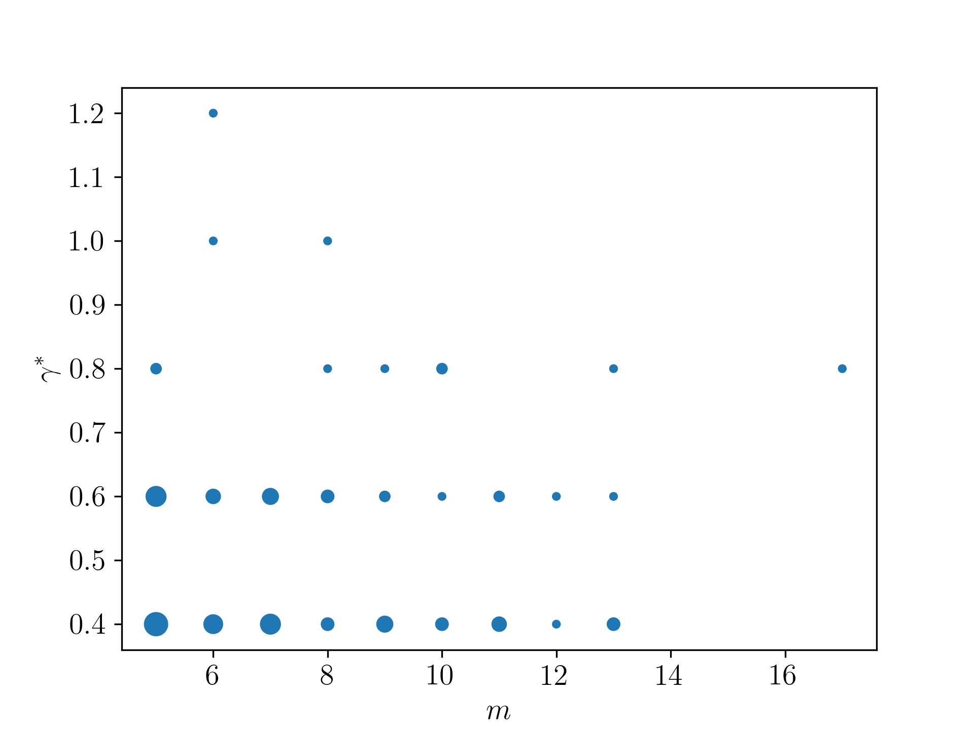
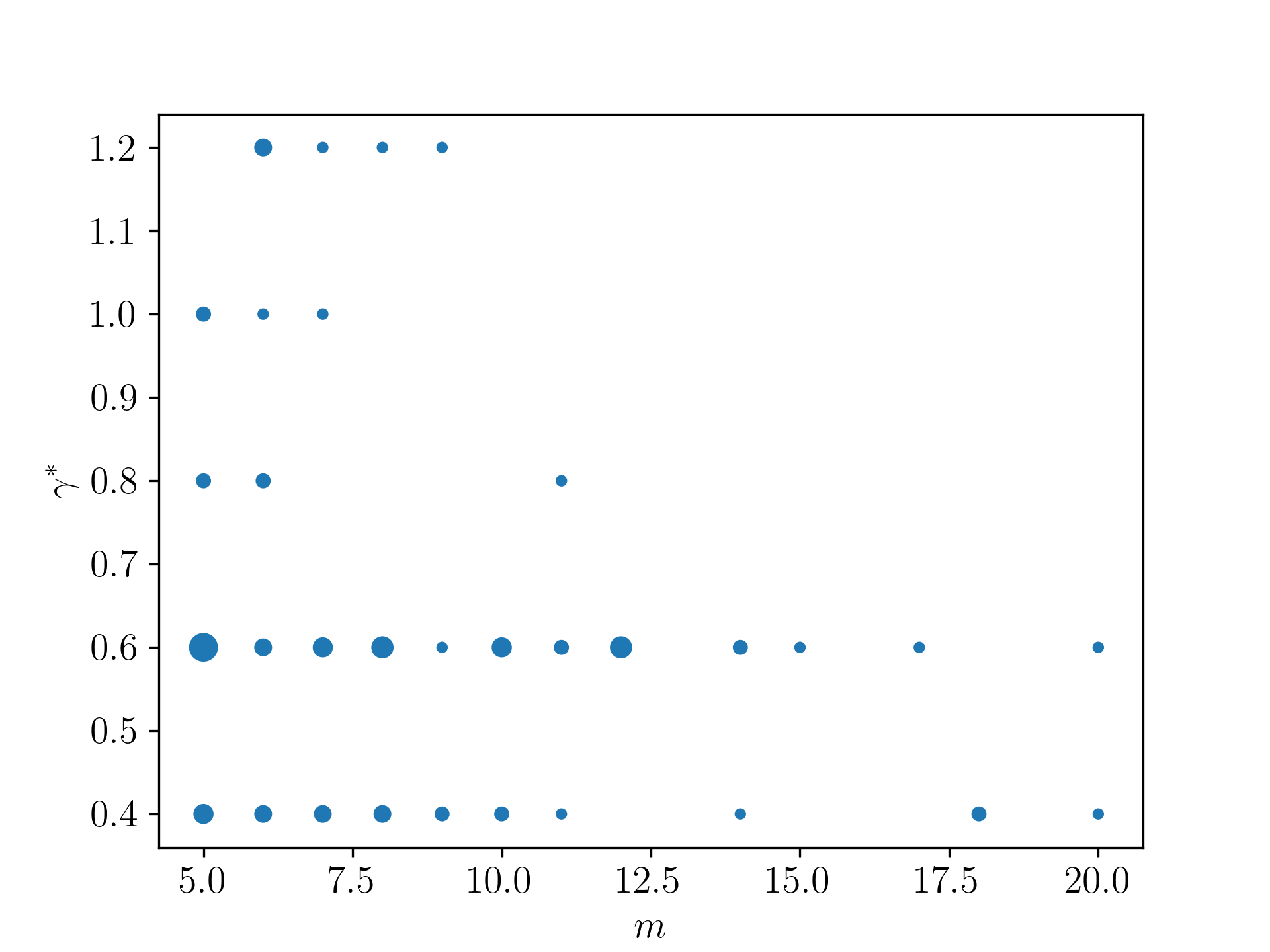
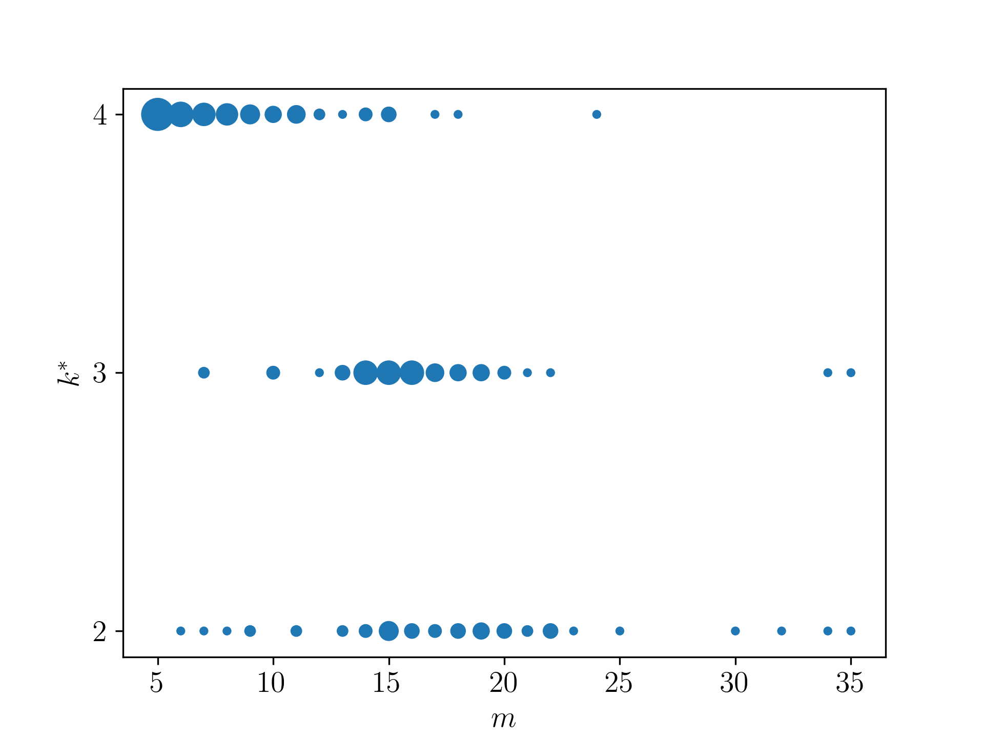
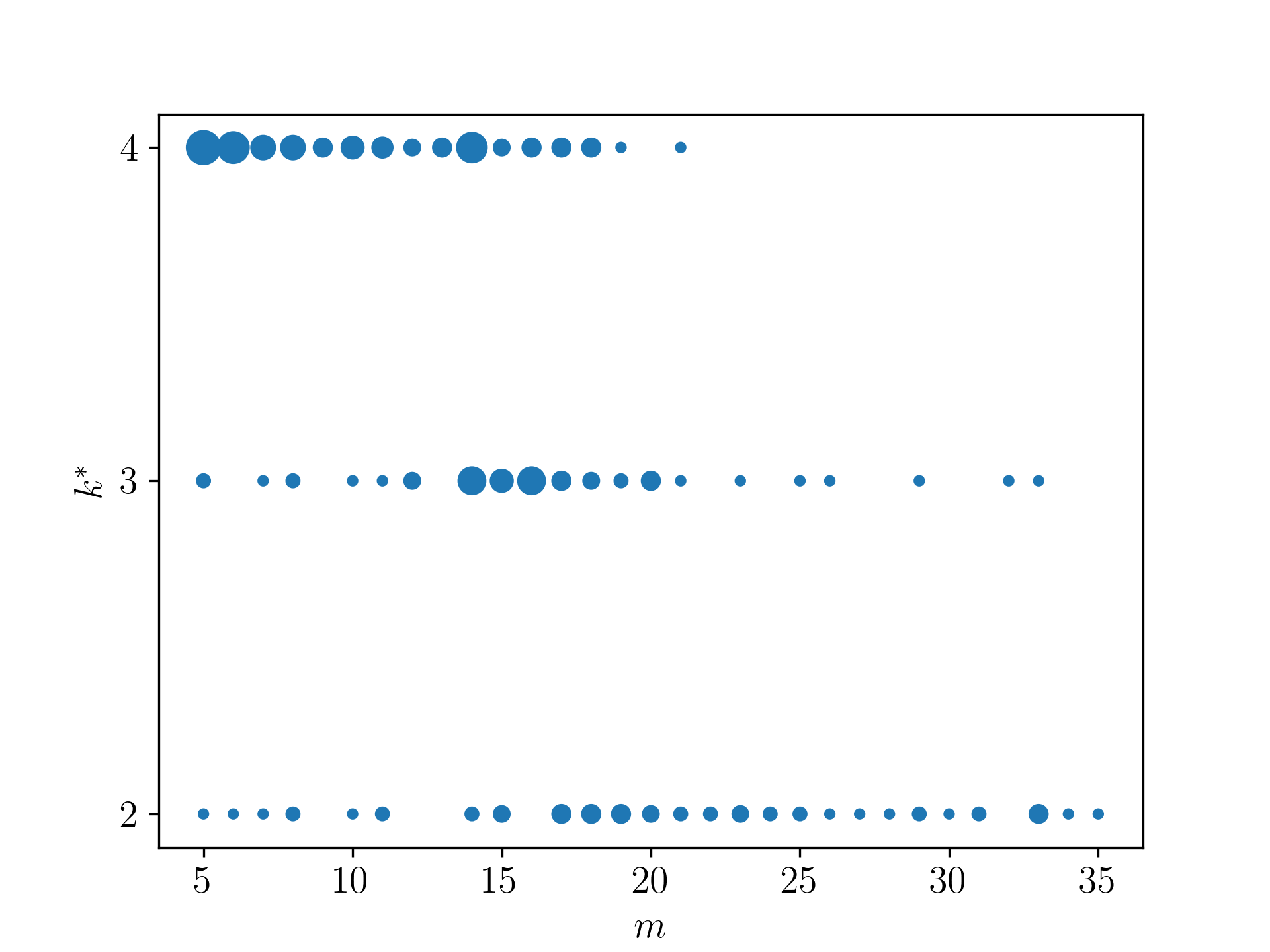
Figure 6 shows the relationship between $m$ and the $\gamma^{*}$ that minimizes $\underline{N}_{\gamma^{*}}$. There are a few blocks for which $\gamma=1.2$ appears to be optimal, but this is often because low-precision estimates for $\lambda_{2}(P_{\gamma=1.2})$ lead to underestimates of $\underline{N}_{\gamma=1.2}$. Computing $\lambda_{2}(P_{\gamma})$ is computationally very expensive for larger values of $\gamma$, which is why we don’t attempt to evaluate $\gamma>1.2$. Figure 7 provides analogous results for the reduced chain, finding that $k=4$ appears to be optimal for smaller blocks, but as blocks get larger, smaller values of $k$ are better.

Disconnected graphs.
Refer to caption
Figure 8: Connected components in the state space of the reduced chain with $k=2$ for a particular block in Alabama (Madison County, tract 2501, block 2053). Dashed purple lines show additional crossing edges present with $k=3$, making the resulting graph connected.

Finally, we consider instances where the reduced chain is not irreducible for $k=2$. Figure 8 shows one such example, where we draw the (undirected) graph given by one-step transitions using $P_{k=2}$. Each node in the graph is some $\mathbf{x}\in\mathcal{X}$. The graph has 3 connected components, and crucially, increasing to $k=3$ adds many crossing edges (shown with purple dashes). Other examples we examined are qualitatively similar, though the density of additional connections with $k=3$ varies.

Appendix F Hardness Results

Existing hardness results for multidimensional knapsack and subset sum do not strictly apply here since (1) we are interested in the decision version, and (2) our solutions can be multisets. However, standard 3SAT reductions to subset sum can be easily adapted to our multidimensional multiset case.

Claim 1.

MMS is NP-hard.

Proof.

Given a 3SAT instance with variables $y_{1},\dots,y_{n}$ and clauses $c_{1},\dots,c_{m}$, we can construct a MMS instance with $2n+3m$ elements and dimension $n+m$ using a slight variant of the standard 3SAT reduction to subset sum. We use the following encoding. For $i\in[n]$,

$\displaystyle\mathbf{v}_{2(i-1)}[j]$ $\displaystyle=\begin{cases}1&j\leq n\wedge i=j\\ 1&j>n\wedge c_{j-n}\text{ contains }y_{i}\\ 0&\text{otherwise}\end{cases}$
$\displaystyle\mathbf{v}_{2i-1}[j]$ $\displaystyle=\begin{cases}1&j\leq n\wedge i=j\\ 1&j>n\wedge c_{j-n}\text{ contains }\overline{y_{i}}\\ 0&\text{otherwise}\end{cases}$
$\displaystyle\mathbf{v}_{2i}[j]$ $\displaystyle=\begin{cases}4&j=2n-1+i\\ 0&\text{otherwise}\end{cases}$
$\displaystyle\mathbf{v}_{2i+1}[j]$ $\displaystyle=\begin{cases}5&j=2n+i\\ 0&\text{otherwise}\end{cases}$
$\displaystyle\mathbf{v}_{2i+2}[j]$ $\displaystyle=\begin{cases}6&j=2n+1+i\\ 0&\text{otherwise}\end{cases}$

Intuitively, the $\mathbf{v}_{i}$ for $i\leq 2n$ represent the variables, with one variable for $y_{i}$ and one for $\overline{y}_{i}$. The remaining $3m$ vectors are slack vectors for the clauses, corresponding to the fact that clause $j$ can be satisfied by 1, 2, or 3 of its variables. Let the counts vector be

$\displaystyle\mathbf{c}[j]=\begin{cases}1&j\leq n\\ 7&j>n\end{cases}$

We will show that this MMS instance is feasible if and only if the original 3SAT instance was feasible.

3SAT solution $\Longrightarrow$ MMS solution. Let $Y_{i}^{*}$ be a 3SAT solution. Let $z_{j}$ be the number of ways in which $c_{j}$ is satisfied by $Y_{i}^{*}$. Note that $z_{j}\in\{1,2,3\}$.

$\displaystyle\mathbf{x}[j]=\begin{cases}1&j\leq 2n\wedge j\text{ is odd}\wedge Y_{(j+1)/2}^{*}=\text{ true}\\ 1&j\leq 2n\wedge j\text{ is even}\wedge Y_{j/2}^{*}=\text{ false}\\ 1&j>2n\wedge j\mod 3=1\wedge z_{(j+2)/3}=3\\ 1&j>2n\wedge j\mod 3=2\wedge z_{(j+1)/3}=2\\ 1&j>2n\wedge j\mod 3=3\wedge z_{(j+1)/3}=1\\ 0&\text{otherwise}\end{cases}$

Observe that $\mathbf{V}\mathbf{x}=\mathbf{c}$ because:

  • For $j\leq n$, $(\mathbf{V}\mathbf{x})[j]=\mathbf{c}[j]$. This is because exactly one of $\mathbf{x}[2i-1],\mathbf{x}[2i]$ can be 1 for $i\leq n$ by construction.

  • For $j>n$, $(\mathbf{V}\mathbf{x})[j]=\mathbf{c}[j]$. This is because for each clause $\ell$, the first $2n$ columns of $\mathbf{V}$ contribute exactly $z_{\ell}$ to $\mathbf{c}[\ell+2n]$. The remaining $3m$ columns contribute $7-z_{\ell}$.

MMS solution $\Longrightarrow$ 3SAT solution. Given a solution $\mathbf{x}$, we assign variables as follows. $y_{i}$ is set to true if $\mathbf{x}[2i-1]=1$ and false if not. We will show that for $j>n$, $\mathbf{V}\mathbf{x}[j]=\mathbf{c}[j]\Longrightarrow$ clause $c_{j-n}$ is satisfied. To see this, note that no multiset consisting of only the last $3m$ columns of $\mathbf{V}$ can sum to $7$, since they only contain the values 4, 5, and 6. Thus, $\mathbf{x}$ must select at least one column from the first $2n$ that has a nonzero entry in position $j$. The only such columns correspond to variables satisfying $c_{j-n}$ (either $\mathbf{v}_{2j-1}$ or $\mathbf{v}_{2j}$). ∎

Appendix G Pathological Examples for the Reduced Chain

Example 2 (Disconnected reduced chain).

In the following example, the reduced chain is disconnected for $k=2$.

$\displaystyle\mathbf{V}=\begin{pmatrix}3&0&0&1\\ 0&3&0&1\\ 0&0&3&1\\ 1&1&1&1\\ \end{pmatrix}$ $\displaystyle\mathbf{c}=\begin{pmatrix}3\\ 3\\ 3\\ 3\end{pmatrix}$

Solutions:

$\displaystyle\mathcal{X}=\left\{\begin{pmatrix}1\\ 1\\ 1\\ 0\end{pmatrix},\begin{pmatrix}0\\ 0\\ 0\\ 3\end{pmatrix}\right\}$

To move between the two solutions in $\mathcal{X}$, we must remove and replace 3 elements at a time, meaning the reduced chain is disconnected for $k=2$. This example can be generalized to be disconnected for any $k<m$.

Example 3 (Connected reduced chain with high mixing time).

Here, we provide an instance $(\mathbf{V},\mathbf{c},\pi)$ such that the reduced chain with $k=2$ is connected but has exponentially large mixing time. Let $\pi$ assign equal probability to all solutions, i.e., $\pi(\mathbf{x})=1/|\mathcal{X}|$. Let $\mathcal{I}_{\ell}$ be the set of $\ell$-dimensional unit basis vectors, i.e., each $\mathbf{e}_{i}\in\mathcal{I}_{\ell}$ has a 1 in the $i$th position and 0 elsewhere. Let $\mathbf{M}_{\ell}\in\mathbb{Z}_{\geq 0}^{\ell\times\left(\ell+\binom{\ell}{2}\right)}$ be the matrix formed by taking as columns all possible sums of two vectors (with replacement) from $\mathcal{I}_{\ell}$ and multiplying them by $\ell$. For example,

$\displaystyle\mathbf{M}_{3}=\begin{pmatrix}6&0&0&3&3&0\\ 0&6&0&3&0&3\\ 0&0&6&0&3&3\end{pmatrix}$

Let $\mathbf{S}_{\ell}\in\mathbb{Z}_{\geq 0}^{\ell\times(\ell-2)}$ be the matrix where column $i\in\{1,\dots,\ell-2\}$ has as its first $i+1$ entries $2\ell$ and 0 elsewhere. For example,

$\displaystyle\mathbf{S}_{3}=\begin{pmatrix}6\\ 6\\ 0\end{pmatrix}$ $\displaystyle\mathbf{S}_{4}=\begin{pmatrix}8&8\\ 8&8\\ 0&8\\ 0&0\end{pmatrix}$

Let $\mathbf{T}_{\ell}\in\mathbb{Z}_{\geq 0}^{\ell\times(2\ell-1)}$ be the matrix where the $i$th column has $i+1$ everywhere. For example,

$\displaystyle\mathbf{T}_{3}=\begin{pmatrix}2&3&4&5&6\\ 2&3&4&5&6\\ 2&3&4&5&6\end{pmatrix}$

Let $\mathbf{1}_{i\times j}$ be the $i\times j$ matrix consisting of all ones. Similarly, let $\mathbf{0}_{i\times j}$ be the matrix consisting of all zeros. Then, define

$\displaystyle\mathbf{V}_{\ell}=\begin{pmatrix}\\ \mathbf{M}_{\ell}&\mathbf{0}_{\ell\times 1}&\mathbf{S}_{\ell}&\mathbf{T}_{\ell}&&\mathbf{1}_{\ell\times\left(\ell+\binom{\ell}{2}\right)}&\mathbf{1}_{\ell\times 1}&\mathbf{1}_{\ell\times(\ell-2)}&\mathbf{1}_{\ell\times(2\ell-1)}\\ &&&&\mathbf{1}_{2\ell\times 1}\\ \mathbf{1}_{\ell\times\left(\ell+\binom{\ell}{2}\right)}&\mathbf{1}_{\ell\times 1}&\mathbf{1}_{\ell\times(\ell-2)}&\mathbf{1}_{\ell\times(2\ell-1)}&&\mathbf{M}_{\ell}&\mathbf{0}_{\ell\times 1}&\mathbf{S}_{\ell}&\mathbf{T}_{\ell}\\ \\ \end{pmatrix}$

For example,

$\displaystyle\mathbf{V}_{3}=\setcounter{MaxMatrixCols}{27}\begin{pmatrix}6&0&0&3&3&0&0&6&2&3&4&5&6&1&1&1&1&1&1&1&1&1&1&1&1&1&1\\ 0&6&0&3&0&3&0&6&2&3&4&5&6&1&1&1&1&1&1&1&1&1&1&1&1&1&1\\ 0&0&6&0&3&3&0&0&2&3&4&5&6&1&1&1&1&1&1&1&1&1&1&1&1&1&1\\ 1&1&1&1&1&1&1&1&1&1&1&1&1&1&6&0&0&3&3&0&0&6&2&3&4&5&6\\ 1&1&1&1&1&1&1&1&1&1&1&1&1&1&0&6&0&3&0&3&0&6&2&3&4&5&6\\ 1&1&1&1&1&1&1&1&1&1&1&1&1&1&0&0&6&0&3&3&0&0&2&3&4&5&6\\ \end{pmatrix}$

Let $\mathbf{c}_{\ell}\in\mathbb{Z}_{\geq 0}^{2\ell}$ have $2\ell$ in each entry. We will show that the reduced chain on the problem defined by $\left(\mathbf{V}_{\ell},\mathbf{c}_{\ell},\pi\right)$ is connected for $k=2$ but has relaxation time exponential in $\ell$. To do so, we upper-bound conductance and use Cheeger’s inequality.

Lemma 10.

The relaxation time of the chain from Example 3 with $k=2$ is $\Omega\left(\left(\frac{\ell}{e}\right)^{\ell}\right)$.

Proof.

Let $\mathcal{V}_{L}$ be the set of columns of $\mathbf{V}_{\ell}$ shown in bold red.

$\displaystyle\mathbf{V}_{\ell}=\begin{pmatrix}\\ {\color[rgb]{1,0,0}\definecolor[named]{pgfstrokecolor}{rgb}{1,0,0}\mathbf{\mathbf{M}_{\ell}}}&{\color[rgb]{1,0,0}\definecolor[named]{pgfstrokecolor}{rgb}{1,0,0}\mathbf{\mathbf{0}_{\ell\times 1}}}&{\color[rgb]{1,0,0}\definecolor[named]{pgfstrokecolor}{rgb}{1,0,0}\mathbf{\mathbf{S}_{\ell}}}&\mathbf{T}_{\ell}&&\mathbf{1}_{\ell\times\left(\ell+\binom{\ell}{2}\right)}&\mathbf{1}_{\ell\times 1}&\mathbf{1}_{\ell\times(\ell-2)}&\mathbf{1}_{\ell\times(2\ell-1)}\\ &&&&\mathbf{1}_{2\ell\times 1}\\ {\color[rgb]{1,0,0}\definecolor[named]{pgfstrokecolor}{rgb}{1,0,0}\mathbf{\mathbf{1}_{\ell\times\left(\ell+\binom{\ell}{2}\right)}}}&{\color[rgb]{1,0,0}\definecolor[named]{pgfstrokecolor}{rgb}{1,0,0}\mathbf{\mathbf{1}_{\ell\times 1}}}&{\color[rgb]{1,0,0}\definecolor[named]{pgfstrokecolor}{rgb}{1,0,0}\mathbf{\mathbf{1}_{\ell\times(\ell-2)}}}&\mathbf{1}_{\ell\times(2\ell-1)}&&\mathbf{M}_{\ell}&\mathbf{0}_{\ell\times 1}&\mathbf{S}_{\ell}&\mathbf{T}_{\ell}\\ \\ \end{pmatrix}$

For example,

$\displaystyle\mathbf{V}_{3}=\setcounter{MaxMatrixCols}{27}\begin{pmatrix}{\color[rgb]{1,0,0}\definecolor[named]{pgfstrokecolor}{rgb}{1,0,0}\mathbf{6}}&{\color[rgb]{1,0,0}\definecolor[named]{pgfstrokecolor}{rgb}{1,0,0}\mathbf{0}}&{\color[rgb]{1,0,0}\definecolor[named]{pgfstrokecolor}{rgb}{1,0,0}\mathbf{0}}&{\color[rgb]{1,0,0}\definecolor[named]{pgfstrokecolor}{rgb}{1,0,0}\mathbf{3}}&{\color[rgb]{1,0,0}\definecolor[named]{pgfstrokecolor}{rgb}{1,0,0}\mathbf{3}}&{\color[rgb]{1,0,0}\definecolor[named]{pgfstrokecolor}{rgb}{1,0,0}\mathbf{0}}&{\color[rgb]{1,0,0}\definecolor[named]{pgfstrokecolor}{rgb}{1,0,0}\mathbf{0}}&{\color[rgb]{1,0,0}\definecolor[named]{pgfstrokecolor}{rgb}{1,0,0}\mathbf{6}}&2&3&4&5&6&1&1&1&1&1&1&1&1&1&1&1&1&1&1\\ {\color[rgb]{1,0,0}\definecolor[named]{pgfstrokecolor}{rgb}{1,0,0}\mathbf{0}}&{\color[rgb]{1,0,0}\definecolor[named]{pgfstrokecolor}{rgb}{1,0,0}\mathbf{6}}&{\color[rgb]{1,0,0}\definecolor[named]{pgfstrokecolor}{rgb}{1,0,0}\mathbf{0}}&{\color[rgb]{1,0,0}\definecolor[named]{pgfstrokecolor}{rgb}{1,0,0}\mathbf{3}}&{\color[rgb]{1,0,0}\definecolor[named]{pgfstrokecolor}{rgb}{1,0,0}\mathbf{0}}&{\color[rgb]{1,0,0}\definecolor[named]{pgfstrokecolor}{rgb}{1,0,0}\mathbf{3}}&{\color[rgb]{1,0,0}\definecolor[named]{pgfstrokecolor}{rgb}{1,0,0}\mathbf{0}}&{\color[rgb]{1,0,0}\definecolor[named]{pgfstrokecolor}{rgb}{1,0,0}\mathbf{6}}&2&3&4&5&6&1&1&1&1&1&1&1&1&1&1&1&1&1&1\\ {\color[rgb]{1,0,0}\definecolor[named]{pgfstrokecolor}{rgb}{1,0,0}\mathbf{0}}&{\color[rgb]{1,0,0}\definecolor[named]{pgfstrokecolor}{rgb}{1,0,0}\mathbf{0}}&{\color[rgb]{1,0,0}\definecolor[named]{pgfstrokecolor}{rgb}{1,0,0}\mathbf{6}}&{\color[rgb]{1,0,0}\definecolor[named]{pgfstrokecolor}{rgb}{1,0,0}\mathbf{0}}&{\color[rgb]{1,0,0}\definecolor[named]{pgfstrokecolor}{rgb}{1,0,0}\mathbf{3}}&{\color[rgb]{1,0,0}\definecolor[named]{pgfstrokecolor}{rgb}{1,0,0}\mathbf{3}}&{\color[rgb]{1,0,0}\definecolor[named]{pgfstrokecolor}{rgb}{1,0,0}\mathbf{0}}&{\color[rgb]{1,0,0}\definecolor[named]{pgfstrokecolor}{rgb}{1,0,0}\mathbf{0}}&2&3&4&5&6&1&1&1&1&1&1&1&1&1&1&1&1&1&1\\ {\color[rgb]{1,0,0}\definecolor[named]{pgfstrokecolor}{rgb}{1,0,0}\mathbf{1}}&{\color[rgb]{1,0,0}\definecolor[named]{pgfstrokecolor}{rgb}{1,0,0}\mathbf{1}}&{\color[rgb]{1,0,0}\definecolor[named]{pgfstrokecolor}{rgb}{1,0,0}\mathbf{1}}&{\color[rgb]{1,0,0}\definecolor[named]{pgfstrokecolor}{rgb}{1,0,0}\mathbf{1}}&{\color[rgb]{1,0,0}\definecolor[named]{pgfstrokecolor}{rgb}{1,0,0}\mathbf{1}}&{\color[rgb]{1,0,0}\definecolor[named]{pgfstrokecolor}{rgb}{1,0,0}\mathbf{1}}&{\color[rgb]{1,0,0}\definecolor[named]{pgfstrokecolor}{rgb}{1,0,0}\mathbf{1}}&{\color[rgb]{1,0,0}\definecolor[named]{pgfstrokecolor}{rgb}{1,0,0}\mathbf{1}}&1&1&1&1&1&1&6&0&0&3&3&0&0&6&2&3&4&5&6\\ {\color[rgb]{1,0,0}\definecolor[named]{pgfstrokecolor}{rgb}{1,0,0}\mathbf{1}}&{\color[rgb]{1,0,0}\definecolor[named]{pgfstrokecolor}{rgb}{1,0,0}\mathbf{1}}&{\color[rgb]{1,0,0}\definecolor[named]{pgfstrokecolor}{rgb}{1,0,0}\mathbf{1}}&{\color[rgb]{1,0,0}\definecolor[named]{pgfstrokecolor}{rgb}{1,0,0}\mathbf{1}}&{\color[rgb]{1,0,0}\definecolor[named]{pgfstrokecolor}{rgb}{1,0,0}\mathbf{1}}&{\color[rgb]{1,0,0}\definecolor[named]{pgfstrokecolor}{rgb}{1,0,0}\mathbf{1}}&{\color[rgb]{1,0,0}\definecolor[named]{pgfstrokecolor}{rgb}{1,0,0}\mathbf{1}}&{\color[rgb]{1,0,0}\definecolor[named]{pgfstrokecolor}{rgb}{1,0,0}\mathbf{1}}&1&1&1&1&1&1&0&6&0&3&0&3&0&6&2&3&4&5&6\\ {\color[rgb]{1,0,0}\definecolor[named]{pgfstrokecolor}{rgb}{1,0,0}\mathbf{1}}&{\color[rgb]{1,0,0}\definecolor[named]{pgfstrokecolor}{rgb}{1,0,0}\mathbf{1}}&{\color[rgb]{1,0,0}\definecolor[named]{pgfstrokecolor}{rgb}{1,0,0}\mathbf{1}}&{\color[rgb]{1,0,0}\definecolor[named]{pgfstrokecolor}{rgb}{1,0,0}\mathbf{1}}&{\color[rgb]{1,0,0}\definecolor[named]{pgfstrokecolor}{rgb}{1,0,0}\mathbf{1}}&{\color[rgb]{1,0,0}\definecolor[named]{pgfstrokecolor}{rgb}{1,0,0}\mathbf{1}}&{\color[rgb]{1,0,0}\definecolor[named]{pgfstrokecolor}{rgb}{1,0,0}\mathbf{1}}&{\color[rgb]{1,0,0}\definecolor[named]{pgfstrokecolor}{rgb}{1,0,0}\mathbf{1}}&1&1&1&1&1&1&0&0&6&0&3&3&0&0&2&3&4&5&6\\ \end{pmatrix}$

Formally, this is

$\displaystyle\mathcal{V}_{L}$ $\displaystyle\triangleq\left\{\mathbf{v}_{i}:i\leq 2\ell+\binom{\ell}{2}-1\right\}$

Let $\mathcal{X}_{L}\subset\mathcal{X}$ be the set of all solutions that only uses elements from $\mathcal{V}_{L}$. Formally, this is

$\displaystyle\mathcal{X}_{L}\triangleq\left\{\mathbf{x}\in\mathcal{X}:\mathbf{x}[i]>0\Longrightarrow i\leq 2\ell+\binom{\ell}{2}-1\right\}.$

Define $\mathcal{X}_{R}$ analogously.

The chain is irreducible.

Observe that $\mathcal{X}_{L}$ is connected to $\mathcal{X}_{R}$ by swaps of size $k=2$: intuitively, starting at a state in $\mathcal{X}_{L}$, we can successively replace elements of $\mathcal{V}_{L}$ with elements from $\mathbf{S}_{\ell}$ and the vector $[0\dots 0~{}1\dots 1]$ until we reach the state with 1 copy of $[2\ell\dots 2\ell~{}1\dots 1]$ and $2\ell-1$ copies of $[0\dots 0~{}1\dots 1]$. From there, we can use elements from $\mathbf{T}_{\ell}$ to reach the solution that consists of $2\ell$ copies of $[1\cdots 1]$. Symmetrically, this state is reachable from $\mathcal{X}_{R}$, meaning the two are connected. More generally, from any solution, by construction the solution consisting of $2\ell$ copies of $[1\cdots 1]$ is reachable.

To bound conductance, we will show that:

  1. 1.

    only one state $\mathbf{x}^{*}\in\mathcal{X}_{L}$ has edges to states in $\mathcal{X}\backslash\mathcal{X}_{L}$,

  2. 2.

    $\pi(\mathbf{x}^{*})/\pi(\mathcal{X}_{L})=1/|\mathcal{X}_{L}|$ is small.

Only one state has crossing edges.

Let $\mathbf{x}^{*}\in\mathcal{X}_{L}$ have an edge to some $\mathbf{x}^{\prime}\notin\mathcal{X}_{L}$. Treating $\mathbf{x}^{*}$ as a multiset, we will reason about the number of copies of each vector $\mathbf{v}$ it contains. We will show that $\mathbf{x}^{*}$ has 1 copy of $[0\cdots 0~{}2\ell~{}1\cdots 1]$, 1 copy of $[2\ell\cdots 2\ell~{}0~{}1\cdots 1]$, and $2\ell-2$ copies of $[0\cdots 0~{}1\cdots 1]$.

Let $\mathbf{v}_{a}$ and $\mathbf{v}_{b}$ be the two elements that can be removed from $\mathbf{x}^{*}$ and replaced by $\mathbf{v}_{c}$ and $\mathbf{v}_{d}$ to yield some $\mathbf{x}^{\prime}\notin\mathcal{X}_{L}$. Let $\mathbf{s}=\mathbf{v}_{a}+\mathbf{v}_{b}$. Observe that the last $\ell$ entries of $\mathbf{s}$ are each 2 because $\mathbf{x}^{*}$ only uses vectors in $\mathcal{V}_{L}$, which all have 1’s in their last $\ell$ entries. Further, observe that each $\mathbf{v}\notin\mathcal{V}_{L}$ has its first $\ell$ entries nonzero and identical. Without loss of generality, let $\mathbf{v}_{c}\notin\mathcal{V}_{L}$. In order for $\mathbf{v}_{a}+\mathbf{v}_{b}=\mathbf{s}=\mathbf{v}_{c}+\mathbf{v}_{d}$, it must be the case that each of the first $\ell$ entries of $\mathbf{s}$ is nonzero, since each of the first $\ell$ entries of $\mathbf{v}_{c}$ is nonzero. For sufficiently large $\ell$ (i.e., $\ell>4$), only three combinations of elements $\mathbf{v}_{a},\mathbf{v}_{b}\in\mathcal{V}_{L}$ have this property. Denoting the first $\ell$ entries of a vector $\mathbf{v}$ as $\mathbf{v}[:\ell]$, these three possible combinations are:

$\displaystyle\mathbf{v}_{a}[:\ell]$ $\displaystyle=\begin{pmatrix}0\\ \vdots\\ 0\\ \ell\\ \ell\end{pmatrix},~{}~{}\mathbf{v}_{b}[:\ell]=\begin{pmatrix}2\ell\\ \vdots\\ 2\ell\\ 0\\ 0\end{pmatrix}$
$\displaystyle\mathbf{v}_{a}[:\ell]$ $\displaystyle=\begin{pmatrix}0\\ \vdots\\ 0\\ \ell\\ \ell\end{pmatrix},~{}~{}\mathbf{v}_{b}[:\ell]=\begin{pmatrix}2\ell\\ \vdots\\ 2\ell\\ 2\ell\\ 0\end{pmatrix}$
$\displaystyle\mathbf{v}_{a}[:\ell]$ $\displaystyle=\begin{pmatrix}0\\ \vdots\\ 0\\ 0\\ 2\ell\\ \end{pmatrix},~{}~{}\mathbf{v}_{b}[:\ell]=\begin{pmatrix}2\ell\\ \vdots\\ 2\ell\\ 2\ell\\ 0\end{pmatrix}$

This yields possible sums for the first $\ell$ entries:

$\displaystyle(\mathbf{v}_{a}+\mathbf{v}_{b})[:\ell]=\mathbf{s}[:\ell]\in\left\{\begin{pmatrix}2\ell\\ \vdots\\ 2\ell\\ \ell\\ \ell\end{pmatrix},\begin{pmatrix}2\ell\\ \vdots\\ 2\ell\\ 3\ell\\ \ell\end{pmatrix},\begin{pmatrix}2\ell\\ \vdots\\ 2\ell\\ 2\ell\\ 2\ell\end{pmatrix}\right\}$

For the first 2 possibilities, it must be the case that the first $\ell$ entries of $\mathbf{v}_{c}$ are identical (because $\mathbf{v}_{c}\notin\mathcal{V}_{L}$) and at most $\ell$ (because otherwise $\mathbf{v}_{d}=\mathbf{s}-\mathbf{v}_{c}$ would contain negative entries). But we can verify that by construction, no $\mathbf{v}_{d}$ exists that yields the desired sum. Thus, the only possible sum is $\mathbf{s}=[2\ell\dots 2\ell~{}2\dots 2]$. Given this choice of $\mathbf{s}$, the only solution that includes the required $\mathbf{v}_{a}$ and $\mathbf{v}_{b}$ must include these two elements and $2\ell-2$ copies of $[0\dots 0~{}1\dots 1]$. This is $\mathbf{x}^{*}$ as claimed.

$\mathcal{X}_{L}$ contains many solutions.

Next, we lower-bound $|\mathcal{X}_{L}|$. A fairly straightforward argument shows $|\mathcal{X}_{L}|\geq 2^{\lfloor\ell/2\rfloor}$. To see this, note that for each pair of indices $i\neq j\leq\ell$, there are two ways to make those entries $2\ell$ and the rest of the first $\ell$ entries 0:

$\displaystyle\begin{pmatrix}2\ell\\ 0\end{pmatrix}+\begin{pmatrix}0\\ 2\ell\end{pmatrix}$ $\displaystyle\begin{pmatrix}\ell\\ \ell\end{pmatrix}+\begin{pmatrix}\ell\\ \ell\end{pmatrix}$

Because there are $\lfloor\ell/2\rfloor$ disjoint pairs of entries in the first $\ell$, there are at least $2^{\lfloor\ell/2\rfloor}$ distinct solutions.

A more sophisticated argument shows that $|\mathcal{X}_{L}|=\Omega\left(\left(\frac{\ell}{e}\right)^{\ell}\right)$. Let $\mathcal{X}_{L}^{\prime}$ be the set of solutions that only use the first $\ell+\binom{\ell}{2}$ columns of $\mathbf{V}_{\ell}$. Since $\mathcal{X}_{L}^{\prime}\subseteq\mathcal{X}_{L}$, $|\mathcal{X}_{L}^{\prime}|\leq|\mathcal{X}_{L}|$. Observe that each of the first $\ell+\binom{\ell}{2}$ columns of $\mathbf{V}_{\ell}$ can be indexed by $(i,j)$ for $i\leq j$, where $\mathbf{v}_{(i,j)}$ is $\ell\times(\mathbf{e}_{i}+\mathbf{e}_{j})$ for unit basis vectors $\mathbf{e}_{i}$ and $\mathbf{e}_{j}$. (A unit basis vector $\mathbf{e}_{i}$ has a 1 in position $i$ and 0 elsewhere.) Any $\mathbf{x}\in\mathcal{X}_{L}^{\prime}$ can thus be expressed as a sequence of these ordered pairs.

Further, any $\mathbf{x}\in\mathcal{X}_{L}^{\prime}$ must have exactly two copies of $\ell\times\mathbf{e}_{i}$ for each $i\in[\ell]$. For some solution $\mathbf{x}\in\mathcal{X}_{L}^{\prime}$, observe that beginning at an arbitrary $\mathbf{v}_{(i,j)}$ in the solution, we can trace out a cycle $i\to j$, $j\to k$, …, $z\to i$ simply by finding the item that provides the matching pair for each $\mathbf{e}_{j}$. Thus, each $\mathbf{x}\in\mathcal{X}_{L}^{\prime}$ uniquely corresponds to a set of (undirected) cycles over $\ell$ elements. (For example, the appearance of $\mathbf{v}_{(i,i)}$ corresponds to a self-loop, and $\mathbf{v}_{(i,j)}$ appearing twice corresponds to a cycle of length 2.) Thus, $|\mathcal{X}_{L}^{\prime}|$ is exactly the number of distinct such collections of cycles.

Defining $a(\ell)$ to be the number of distinct collections of cycles over $\ell$ elements, Stanley (1999, Example 5.2.9) shows that $a(\ell)$ satisfies

$\displaystyle\sum_{\ell\geq 0}a(\ell)\frac{x^{\ell}}{\ell!}=(1-x)^{-1/2}\exp\left(\frac{x}{2}+\frac{x^{2}}{4}\right).$

The sequence $a(0),a(1),\dots$ appears as OEIS sequence A002135 (OEIS Foundation Inc., 2023), and satisfies the recurrence $a(\ell)=\ell\cdot a(\ell-1)-\binom{\ell-1}{2}a(\ell-3)$. Asymptotically (c.f. Pietro Majer (OEIS Foundation Inc., 2023)),

$\displaystyle a(\ell)\sim\sqrt{2}\exp\left(\frac{3}{4}\right)\left(\frac{\ell}{e}\right)^{\ell}\left(1+O\left(\frac{1}{\ell}\right)\right).$

Thus, $|\mathcal{X}_{L}|\geq|\mathcal{X}_{L}^{\prime}|=a(\ell)=\Omega\left(\left(\frac{\ell}{e}\right)^{\ell}\right)$.

Conductance and Cheeger’s inequality.

With this, we are ready to bound the chain’s conductance and thus its relaxation time. We need the following definitions. For our Markov chain $M_{\ell}$ with transition matrix $P_{\ell}$,

$\displaystyle Q_{\ell}(\mathbf{x},\mathbf{x}^{\prime})$ $\displaystyle\triangleq\pi(\mathbf{x}^{\prime})P_{\ell}(\mathbf{x},\mathbf{x}^{\prime})$
$\displaystyle Q_{\ell}(\mathcal{S},\overline{\mathcal{S}})$ $\displaystyle\triangleq\sum_{\mathbf{x}\in\mathcal{S},\mathbf{x}^{\prime}\notin\mathcal{S}}Q_{\ell}(\mathbf{x},\mathbf{x}^{\prime})$
$\displaystyle\Phi(\mathcal{S},\overline{\mathcal{S}})$ $\displaystyle\triangleq\frac{Q_{\ell}(\mathcal{S},\overline{\mathcal{S}})}{\pi(\mathcal{S})}$
$\displaystyle\Phi(M_{\ell})$ $\displaystyle\triangleq\min_{\mathcal{S}:0<\pi(\mathcal{S})\leq 1/2}\Phi(\mathcal{S},\overline{\mathcal{S}})$
$\displaystyle\leq\Phi(\mathcal{X}_{L},\overline{\mathcal{X}_{L}})$
$\displaystyle=\frac{\sum_{\mathbf{x}\in\mathcal{X}_{L},\mathbf{x}^{\prime}\notin\mathcal{X}_{L}}\pi(\mathbf{x})P_{\ell}(\mathbf{x},\mathbf{x}^{\prime})}{\pi(\mathcal{X}_{L})}$
$\displaystyle\leq\frac{\sum_{\mathbf{x}\in\mathcal{X}_{L},\mathbf{x}^{\prime}\notin\mathcal{X}_{L}}\pi(\mathbf{x})}{\pi(\mathcal{X}_{L})}$ ($P_{\ell}(\cdot,\cdot)\leq 1$)
$\displaystyle=\frac{\pi(\mathbf{x}^{*})}{\pi(\mathcal{X}_{L})}$ ($\mathbf{x}^{*}$ is the only state with a crossing edge)
$\displaystyle=\frac{1}{|\mathcal{X}_{L}|}$ ($\pi(\mathbf{x})\propto 1$)
$\displaystyle=O\left(\left(\frac{e}{\ell}\right)^{\ell}\right)$

By Cheeger’s inequality (Jerrum and Sinclair, 1988; Lawler and Sokal, 1988),

$\displaystyle\lambda_{2}(P_{\ell})\geq 1-2\Phi(M_{\ell}).$

This means that

$\displaystyle\tau_{\mathrm{rel}}(P_{\ell})=\frac{1}{1-\lambda_{2}(P_{\ell})}\geq\frac{1}{2\Phi(M_{\ell})}=\Omega\left(\left(\frac{\ell}{e}\right)^{\ell}\right).$

Appendix H Final Algorithm Description

Algorithm 4 ILPandMCMC($\mathbf{V},\mathbf{c},f,N,k,t$)
$\mathcal{S}\leftarrow$ subset of $\mathcal{X}$ of size at most $N$ $\triangleright$ Using ILP, with objective $L(\cdot)$ given by 17
$\mathbf{x}\leftarrow$ a random $\mathbf{x}\in\mathcal{S}$ according to $\pi\;|\;\mathbf{x}\in\mathcal{S}$
if $|\mathcal{S}|<N$ then $\triangleright$ In this case, $(\pi\;|\;\mathbf{x}\in\mathcal{S})=\pi$
     return 𝐱𝐱\mathbf{x}
else
     return Reduced($\mathbf{V},\mathbf{c},f,k,t,\mathbf{x}$)
end if

Recall that our upper bounds on $N_{k}$ relied on the fact that $\pi(\mathbf{x}_{0})\geq 1/|\mathcal{X}|$. This may no longer be true when $\mathbf{x}_{0}$ is sampled from $\pi\;|\;\mathbf{x}\in\mathcal{S}$. Here, we provide a bound that only depends on $\pi(\mathcal{S})$, not $|\mathcal{X}|$. As long as $\pi(\mathcal{S})\geq 1/|\mathcal{X}|$, our new bound is stronger. See 9

Proof.

Let $\mathbb{X}\sim\pi_{0}$ where $\pi_{0}=\pi\;|\;\mathbf{x}\in\mathcal{S}$. Let $P_{k}^{t}(\mathbb{X},\cdot)$ be the distribution of over the reduced chain beginning with $\mathbb{X}$ after $t$ steps. Following Sousi (2020, Theorem 3.4), for a reversible Markov chain with transition matrix $P_{k}$ and relaxation time $\tau_{\mathrm{rel}}$,

$\displaystyle\|P_{k}^{t}(\mathbb{X},\cdot)-\pi\|_{2,\pi}\leq\exp(-t/\tau_{\mathrm{rel}})\|\pi_{0}-\pi\|_{2,\pi},$ (21)

where given a stationary distribution $\pi$, we define

$\displaystyle\|\sigma-\pi\|_{2,\pi}\triangleq\left(\sum_{\mathbf{x}\in\mathcal{X}}\left(\frac{\sigma(\mathbf{x})}{\pi(\mathbf{x})}-1\right)^{2}\pi(\mathbf{x})\right)^{1/2}.$

For initial distribution $\pi_{0}=\pi\;|\;\mathbf{x}\in\mathcal{S}$,

$\displaystyle\|\pi_{0}-\pi\|_{2,\pi}^{2}$ $\displaystyle=\sum_{\mathbf{x}\in\mathcal{X}}\left(\frac{\pi_{0}(\mathbf{x})}{\pi(\mathbf{x})}-1\right)^{2}\pi(\mathbf{x})$
$\displaystyle=\sum_{\mathbf{x}\in\mathcal{X}}\left(\frac{\pi_{0}(\mathbf{x})^{2}}{\pi(\mathbf{x})^{2}}-\frac{2\pi_{0}(\mathbf{x})}{\pi(\mathbf{x})}+1\right)\pi(\mathbf{x})$
$\displaystyle=\sum_{\mathbf{x}\in\mathcal{X}}\frac{\pi_{0}(\mathbf{x})^{2}}{\pi(\mathbf{x})}-2\pi_{0}(\mathbf{x})+\pi(\mathbf{x})$
$\displaystyle=\left(\sum_{\mathbf{x}\in\mathcal{X}}\frac{\pi_{0}(\mathbf{x})^{2}}{\pi(\mathbf{x})}\right)-1$
$\displaystyle=\left(\sum_{\mathbf{x}\in\mathcal{S}}\frac{\pi_{0}(\mathbf{x})^{2}}{\pi(\mathbf{x})}+\sum_{\mathbf{x}\notin\mathcal{S}}\frac{\pi_{0}(\mathbf{x})^{2}}{\pi(\mathbf{x})}\right)-1$
$\displaystyle=\left(\sum_{\mathbf{x}\in\mathcal{S}}\frac{(\pi(\mathbf{x})/\pi(\mathcal{S}))^{2}}{\pi(\mathbf{x})}\right)-1$
$\displaystyle=\left(\sum_{\mathbf{x}\in\mathcal{S}}\frac{\pi(\mathbf{x})}{\pi(\mathcal{S})^{2}}\right)-1$
$\displaystyle=\frac{1}{\pi(\mathcal{S})}-1$
$\displaystyle\leq\frac{1}{\pi(\mathcal{S})}.$

Thus, by 21,

$\displaystyle\|P_{k}^{t}(\mathbb{X},\cdot)-\pi\|_{2,\pi}\leq\exp(-t/\tau_{\mathrm{rel}})\frac{1}{\sqrt{\pi(\mathcal{S})}}.$ (22)

Next, observe that for any $\sigma$,

$\displaystyle\|\sigma-\pi\|_{1}^{2}$ $\displaystyle=\left(\sum_{\mathbf{x}\in\mathcal{X}}|\sigma(\mathbf{x})-\pi(\mathbf{x})|\right)^{2}$
$\displaystyle=\left(\sum_{\mathbf{x}\in\mathcal{X}}\left|\frac{\sigma(\mathbf{x})}{\pi(\mathbf{x})}-1\right|\pi(\mathbf{x})\right)^{2}$
$\displaystyle\leq\sum_{\mathbf{x}\in\mathcal{X}}\left(\frac{\sigma(\mathbf{x})}{\pi(\mathbf{x})}-1\right)^{2}\pi(\mathbf{x})$ (Jensen’s inequality)
$\displaystyle=\|\sigma-\pi\|_{2,\pi}^{2}.$

Combining this with 22,

$\displaystyle 2d_{\mathrm{TV}}(P_{k}^{t}(\mathbb{X},\cdot),\pi))=\|P_{k}^{t}(\mathbb{X},\cdot)-\pi\|_{1}\leq\|P_{k}^{t}(\mathbb{X},\cdot)-\pi\|_{2,\pi}\leq\exp(-t/\tau_{\mathrm{rel}})\frac{1}{\sqrt{\pi(\mathcal{S})}}.$

To achieve the desired bound on $d_{\mathrm{TV}}(P_{k}^{t}(\mathbb{X},\cdot),\pi)$, it suffices to set

$\displaystyle\frac{1}{2}\exp(-t/\tau_{\mathrm{rel}})\frac{1}{\sqrt{\pi(\mathcal{S})}}$ $\displaystyle\leq\varepsilon$
$\displaystyle\exp(-t/\tau_{\mathrm{rel}})$ $\displaystyle\leq 2\varepsilon\sqrt{\pi(\mathcal{S})}$
$\displaystyle t$ $\displaystyle\geq\tau_{\mathrm{rel}}\log\left(\frac{1}{2\varepsilon\sqrt{\pi(\mathcal{S})}}\right)$