A fully Bayesian approach for the imputation and analysis of derived outcome variables with missingness
Abstract
Derived variables are variables that are constructed from one or more source variables through established mathematical operations or algorithms. For example, body mass index (BMI) is a derived variable constructed from two source variables: weight and height. When using a derived variable as the outcome in a statistical model, complications arise when some of the source variables have missing values. In this paper, we propose how one can define a single fully Bayesian model to simultaneously impute missing values and sample from the posterior. We compare our proposed method with alternative approaches that rely on multiple imputation, and, with a simulated dataset, consider how best to estimate the risk of microcephaly in newborns exposed to the ZIKA virus.
Keywords: multiple imputation, missingness, Bayesian inference.
1 Introduction
‘Derived variables’ are variables that are constructed from one or more measured variables through established mathematical operations or algorithms. Examples of commonly used derived variables include body mass index (BMI), constructed from weight and height, and the 36-Item Short Form Health Survey Physical Component Summary score (SF-36 PCS), constructed from a combination of responses measured on the 36-Item Short Form Survey (SF-36).
When using a derived variable, a particular complication may arise when some of the measured ‘source’ variables required to derive it have missing values. Missingness in source variables will often lead to missingness in derived variables. For example, if weight is missing for certain study participants, their BMI cannot be derived. However, this is not quite the same as having completely-missing information on the derived variable. In some instances, one might have some information. For example, if a single question on the SF-36 is left unanswered, one might still be able to infer, at least approximately, a participant’s SF-36 PCS based on their answers to the other 35 questions. More clearly, if a composite outcome is defined to be 1 if either component is 1, then observing that one component equals 1 means the composite is known whether or not the other component is measured (Pham et al. 2021).
The data that motivated this work consists of measurements taken from newborns of mothers infected with the ZIKA virus (Wilder-Smith et al. 2019). In order to determine if the newborns have microcephaly (a derived variable), a calculation based on three source variables (sex, gestational age, and head circumference) is required. The source variables are often subject to missingness and we were curious as to how one might be able to fit these data with an entirely Bayesian solution.
Besides the so-called complete-case analysis, in which observations with any missing values are discarded, the most popular statistical approach for handling missing data is multiple imputation (MI) (Rubin 1976, Reiter & Raghunathan 2007) and among the different varieties of MI, the Multivariate Imputation by Chained Equations (MICE) approach is the most widely used (Van Buuren 2018). The basic idea of MI is to fill in missing values by repeated simulation from the posterior predictive distributions of the missing values given assumptions about the missing data mechanism and a model, thereby preserving the uncertainty associated with the missingness. MICE does this for multivariate non-monotone missing data variables by using a sequence of univariate conditional distributions (i.e., imputing variables one-at-a-time).
When using MICE to impute missing values of derived variables, there are three general approaches:
-
1.
imputation at the derived-variable level (DVL), in which one imputes the derived variable directly ignoring the source variables;
-
2.
imputation at the source-variable level (SVL), in which one imputes the source variables first and then computes the derived variable afterwards (also known as the impute, then transform approach); and
-
3.
the just another variable (JAV), approach, in which one imputes the source variables and derived variable together, with the source variables as covariates in the imputation model for the derived variable.
There are two other approaches we should mention that have been studied in the literature but are not necessarily relevant for our situation. The first is known as “on-the-fly” imputation, where the transformation of the source variables into the derived variable is done “on-the-fly” within the imputation algorithm. (Note that Van Buuren (2018) calls this “passive imputation”). This can be advantageous when there are observations for which the derived variable is observed but the source variables are missing (e.g., there are individuals with known BMI, but unknown height and/or weight). We will assume that missingness in source variables necessarily implies missingness in the derived variable (e.g., any individual with unknown height or weight will necessarily have unknown BMI). In this case, on-the-fly imputation is entirely equivalent to SVL imputation. The other approach we should mention, proposed by Bartlett et al. (2015), is known as the Substantive Model Compatible Fully Conditional Specification (SCMFCS) imputation. This method is useful for imputing derived covariate values, but not derived outcome variables (which is our focus).
Because DVL imputation effectively excludes information available in the source variables (which are possibly the best predictors of the missing derived variable values), SVL imputation is thought to be a more efficient strategy, in the sense that it uses observed information where possible. Pan et al. (2020) compare the performance of the two approaches and conclude that SVL imputation is indeed preferable, regardless of how the derived variable is obtained (“whether by simple arithmetic operations or by some highly specific algorithms”). This follows related work by Gottschall et al. (2012) who arrived at a similar conclusion for handling missing values in questionnaire data (“researchers should adopt item-level imputation whenever possible”).
| (source) | (source) | (derived) | ||
|---|---|---|---|---|
| Pattern 1 | Missing | Observed | Missing | |
| Pattern 2 | Observed | Missing | Missing | |
| Pattern 3 | Missing | Missing | Missing |
Another reason to favour the SVL and JAV approaches over DVL imputation is that they make a less restrictive MAR (missing at random) assumption. MAR requires that the conditional probability of missingness depends only on data observed under that pattern (Rubin 1976). Consider for example a derived outcome that is equal to the sum of two source variables, and , such that . Missingness in can occur in three patterns: First, the value is missing, second the value is missing, third, both and values are missing; see Table 1. Because MAR is i) defined at the observation level rather than at the variable level, and ii) conditional on variables included in the analysis, we see that assuming MAR with DVL imputation requires that missingness in the derived variable be independent of the value of under any pattern. For the SVL and JAV approaches, this is relaxed under patterns 1 and 2: missingness in under pattern 1 need only be independent of , not , and missingness in under pattern 2 need only be independent of , not .
| The MAR assumption requires that, under this | |||
| pattern, missingness in is independent of | |||
| (source) | (source) | (derived) | |
| Pattern 1: | - | ||
| Pattern 2: | - | ||
| Pattern 3: | |||
To conduct Bayesian inference with imputed data, Gelman et al. (2004) outline a three step procedure. The first step is to construct several imputed datasets, using MI. The second step is to simulate draws from the posterior distribution with each imputed dataset separately. The third and final step is to mix all the draws together, thereby obtaining (at least approximately) draws from the posterior distribution that take into account the uncertainty associated with the missing data; see Zhou & Reiter (2010). (This third step is perhaps surprising to those familiar with multiple imputation inference: Rubin’s combining rules are not needed.) While Gelman et al. (2004)’s three step procedure appears straightforward, when SVL imputation is used for imputing a derived outcome variable, things can be much more complicated. This becomes apparent when considering the assumptions required in the first two steps.
Using SVL imputation in the first step requires one to specify distributions for each of the missing source variables. Then, specifying the posterior distribution in second step requires one to define a distribution – along with priors for the parameters that characterize the distribution – for the derived outcome variable. Clearly the assumed distributions of the source variables (specified in step 1) necessarily determine the distribution of the derived outcome variable (which must be specified in step 2). Without careful consideration, one could inadvertently define incompatible distributions, since the two steps are done separately and the software implementing one step (e.g., MICE from van Buuren et al. (2015)) does not know of the assumptions required by the other step (e.g., rstan from Carpenter et al. (2017)). Moreover, it will no doubt be difficult to determine whether or not the assumptions made by the Bayesian model specified in the second step (e.g., regarding priors) are consistent with the assumptions made when imputing missing values in the first step.
Ideally, one could fit a single fully Bayesian model to simultaneously impute missing values and sample from the posterior. The idea of avoiding potential problems with MI by adopting a fully Bayesian approach is not new and it is actually quite common to proceed in this way when covariate values are missing; see Bartlett et al. (2015) and Erler et al. (2021) and the references therein. However, it is not at all obvious how to proceed when there is missingness in source variables that combine to define a derived outcome variable. In this article, we propose a useful approach.
In Section 2, we begin with a simple illustrative example. In Section 3, we outline our proposed approach. In Section 4, we consider how best to estimate the risk of microcephaly in newborns exposed to the ZIKA virus with an artificial dataset. Finally, we conclude in Section 5.
2 Illustrative example
We continue with the simple example discussed in the introduction where . Suppose we are interested in two groups, group and group , (e.g., placebo and treatment) and we are interested in estimating , the difference between , the expectation of in group , and , the expectation of in group : . The easiest way to proceed might be to fit a simple univariate Normal model for where, for :
where
with priors specified for , and .
Now suppose that, in group , a proportion of and values are missing. Specifically, in group , certain observations are prone to have missing values with the chance of missingness depending on , and other observations are prone to have missing values with the chance of missingness depending on the observed . (To be clear, in this specific example, no observations are susceptible to missing both and .) Table 3 lists the data for six individuals to illustrate, with “NA” indicating missing. Given this missingness in the data, how should we proceed to estimate ?
| Group | ||||
|---|---|---|---|---|
| 1 | A | NA | NA | 1.71 |
| 2 | A | 1.59 | 0.08 | 1.68 |
| 3 | A | NA | 1.23 | NA |
| 4 | B | 2.40 | 2.20 | 0.20 |
| 5 | B | 4.49 | 2.35 | 2.14 |
| 6 | B | 3.53 | 0.49 | 3.03 |
As discussed in the introduction, one could consider the complete-case analysis in which case, all rows of data with any missing values would be discarded (e.g., individuals and listed in Table 3 would be discarded). The advantage of this strategy is that no imputation step is required and the entire procedure is to simply fit the univariate Normal model. The disadvantage is that this strategy almost certainly involves a loss of efficiency and has the potential for bias.
Alternatively, one could apply Gelman’s three step procedure with one of the three MICE approaches (either the DVL, SVL, or JAV imputation methods) for imputing the missing values followed by the univariate Normal model for inference. The advantage of this strategy is that, depending on the specific MICE approach used, one could conceivably obtain unbiased estimates of in an efficient manner. The disadvantage is that this strategy involves two separate steps (an imputation step and an inference step) which may not be consistent with one another.
There is another possible strategy worth considering. Because the math in this scenario is rather simple, one could fit a Bayesian model for the source variables, and , and derive samples of based on samples of and . For instance, we could fit a bivariate Normal model for and , where, for in 1,…,:
| (1) |
where
| and, for each MCMC iteration, | compute | |||
| (2) |
Priors would need to be specified for each of the seven parameters: , , , , and .
This strategy might be ideal in the sense that it does not require a separate imputation step (the entire procedure is to simply fit the bivariate Normal model) and does not disregard a large number of observations. However, we this strategy is possible only because in this illustrative example the math is extremely straightforward (i.e., equation (2) is known). For other derived variables, this might not be the case. For instance, if instead of , we had , then computing from a combination of the seven other parameters might be impossible without a certain degree of mathematical wizardry.
This brings us to our proposed method, details of which are provided in the next section. Briefly, the approach involves using Monte Carlo integration to derive samples of the derived outcome variable. In our example this would involve fitting the bivariate Normal model and sampling (at least approximately) without requiring any knowledge about the mathematical derivation of .
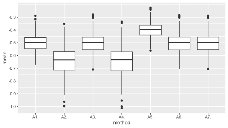
Before continuing on with more details, let us review the results of a small simulation study to confirm that our intuitions regarding each of the possible strategies in the illustrative example are acceptable. We simulated 500 datasets of size and applied each of the six methods (details are in the Appendix). The aim was to demonstrate a proof-of-concept for our proposed method (A7). Five hundred complete-data observations were generated as
| if is in group | ||||
Subsequently, missingness was imposed under a missing-at-random mechanism. All data remained fully observed for group . For group , 250 observations had non-zero probability of being missing and the other 250 had non-zero probability of being missing. The following models determined the probability of missingness in these two subsets.
For analysis of the incomplete data, each of the MICE methods was used to produce 50 imputed datasets, each Bayesian model was fit using MCMC with draws, and the proposed method was implemented with Monte Carlo samples for the integration. We also analysed data prior to introduction of missingness (i.e., from the oracle) and fit the univariate normal model to these data. Figure 1 shows the results. In summary, we see that:
-
•
The complete-case analysis (A2) and the three-step approach with DVL imputation (A4) are both biased as expected, since the data generating mechanism is not MCAR.
-
•
The three-step approach with SVL imputation (A3) is unbiased.
-
•
Both approaches that fit the bivariate Normal model (A6 and A7) are unbiased and just as efficient as the three-step approach with SVL imputation (A3).
-
•
Finally, the three-step approach with JAV (A5) imputation appears to be biased. This is surprising, since in this case JAV imputation should be identical to SVL imputation. A brief explanation of this claim is given in the Appendix. In short, this is not a property of JAV imputation but of the R package {mice} used to implement it.
3 Description of the approach
Having established the motivation behind our proposed method, we now outline the details more specifically. Note that, while we outline the method as it applies to an analysis in which the objective is to determine the relationship between a derived outcome variable and a single binary exposure variable, the method could be modified as needed to suit other scenarios.
For the -th observation in =1,…,, let be the exposure variable, be the derived outcome variable, and be source variables, such that , for some deterministic function . For instance, in the earlier example, was the “group” membership and the function defined the addition of source variables: .
Suppose is the estimand of interest and the primary goal is in determining the posterior distribution of . In the earlier example, interest was in determining the difference in the mean of between individuals in the two groups, such that .
Now suppose that there is missingness for various values of , and that that we know (or can safely assume) the conditional distribution for the source variables, . This is the key assumption on which our proposal rests. Let be all the parameters describing the distribution and let be a function (perhaps unknown) such that . In the previous example, a bivariate Normal model was specified for (see equation (1)), consisted of seven parameters (, , , , and ), and was known and defined as: (see equation (2)).
The standard Bayesian approach would be to obtain a Monte Carlo sample of size (e.g., via MCMC) from the posterior distribution and then, if is known, obtain posterior samples of by applying the function to the posterior samples of . (In the previous section, this was the A6 “Bivariate Normal model (with math)” approach). Instead, our proposal is to create an additional variable, , for each of the source variables. For in 1,…,, we define such that its distribution is identical to that of . However, whereas is partially (or entirely) observed, is entirely unobserved. In this sense, could be understood as “future observations projected by the model” of . With a sufficiently large number of draws of , the distribution of should accurately approximate that of .
By then applying the deterministic function on samples of , one can obtain samples of , a new variable with the same identical distribution as (i.e., “future observations projected by the model” of the variable). Then, one can obtain posterior samples of based on the values. Obtaining samples of from in this fashion ensures that the correct amount of variation is captured and, importantly, does not require knowledge of the function . To be clear, our approach consists of the following four steps:
-
1.
Draw samples of from the distribution: , for in 1,…,.
-
2.
For in 1,…,, draw iid samples from the distribution: , for in 1,…, ; and iid samples from the distribution: , for in 1,…, .
-
3.
Apply the deterministic function to the samples obtained in step 2 to obtain iid samples from the distribution: , for in 1,…, ; and iid samples from the distribution: , for in 1,…, .
-
4.
Use the samples obtained in step 3 to numerically approximate a draw of , for in 1,…,. Note that approaching equality with sufficiently large . For instance, in our earlier example we had , and would substitute the two expectations with their respective sample means, such that:
(3) for in 1,…,.
Having obtained posterior samples of following these four steps, one can then calculate a posterior median/mean and credible interval for , as is standard practice in a Bayesian analysis. Both and should be sufficiently large that both sources of Monte Carlo error are negligible. In the next section we demonstrate how this approach can be applied in the motivating application.
4 Application to data: Estimating the risk of microcephaly
Background
Zika virus infection (ZIKV) during pregnancy is known to be associated with an increased risk of fetal congenital malformations, including microcephaly, a birth condition in which a baby’s head is smaller than expected when compared to babies of the same sex and age. Formally, microcephaly is defined as a measure of head circumference at birth of more than 2 standard deviations below average for sex and gestational age; see Harville et al. (2020). (Average values for head circumference at birth can be determined by referencing the standards calculated by the intergrowth-21st research network; see Villar et al. (2014)). Therefore, in a healthy population, we would anticipate 2.28% of newborns being categorized as having microcephaly (assuming head circumference in the general population is Gaussian).
In order to determine the risk of microcephaly associated with ZIKV, observational data has been collected by numerous studies from infected pregnant women (Zika Virus Individual Participant Data Consortium 2020). These data typically suffer from substantial missingness.
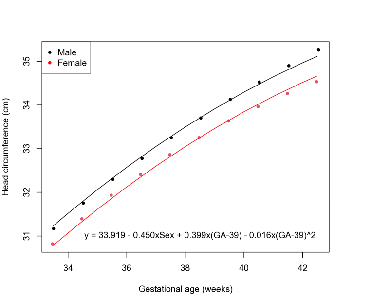
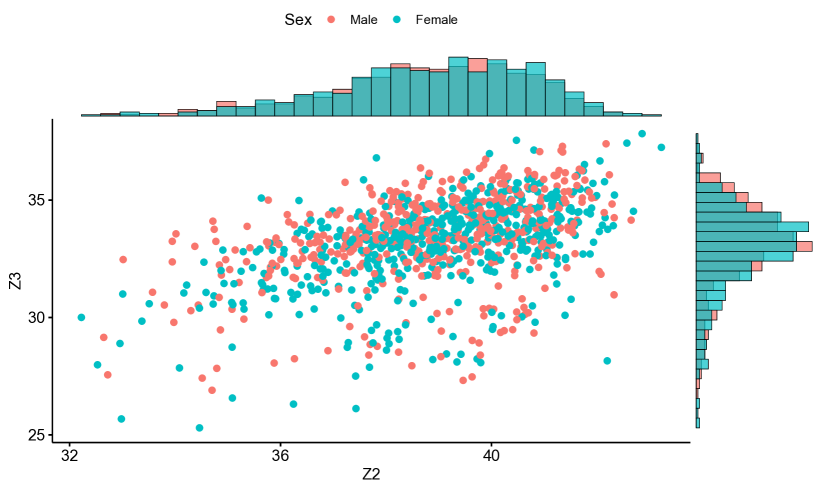
The outcome of interest, microcephaly (), is a derived binary variable, based on three source variables: (1) sex (=0 for ‘male’ and =1 for ‘female’), (2) gestational age (, measured in weeks), and (3) head circumference (, measured in centimetres). Each of these three source variables is subject to missingness. The exposure variable is maternal ZIKV status () but in this example the data we consider only include subjects for whom . Specifically, we consider a simple artificial dataset based on what is typically observed in observational studies. The data is simulated with a “true” risk of microcephaly of = 11.69%. Missing values are attributed completely at random, missing values are more likely for those with very small values of , and missing values are more likely for those with very large values of .
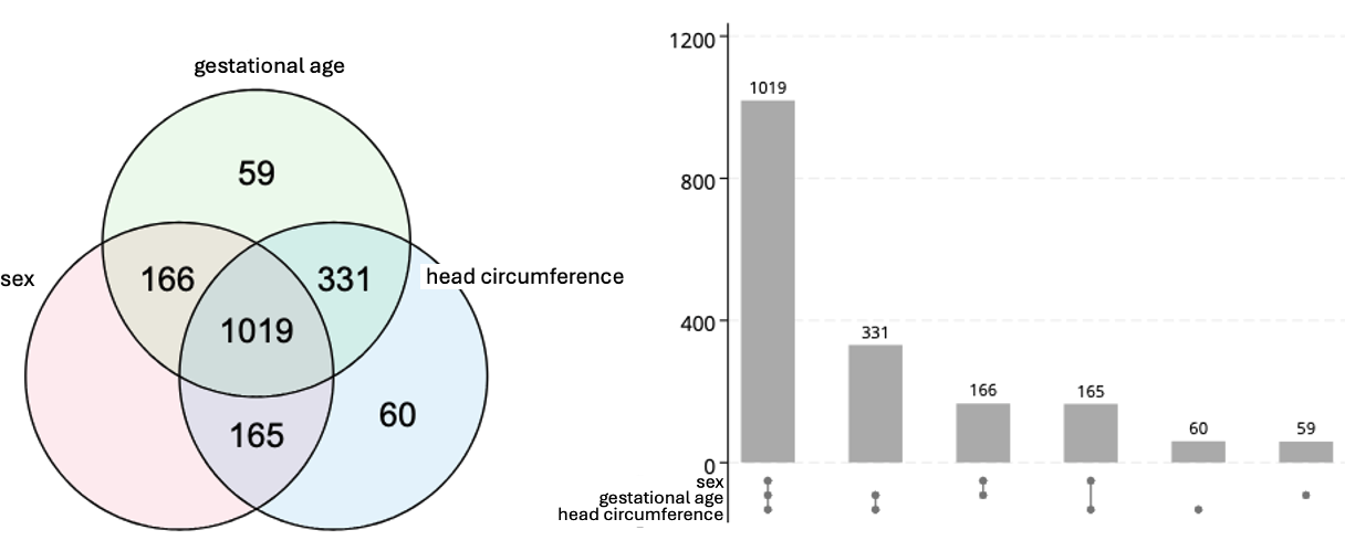
The data and models
The data consist of , , and values (when available) from newborns; see Figure 2. There are 781 individuals who have at least one value missing; see Venn diagram in Figure 3. Microcephaly status, , for a newborn can be calculated by first deriving their “z-score” based on their head circumference, gestational age and sex. (The “igb_hcircm2zscore” function in the growthstandards R package can do this easily using the intergrowth standards). If a newborn’s z-score is below , they are classified as having microcephaly. As such, while the function is known and can be easily applied to the source variables to obtain the binary derived variable, it is not easily written out.
We consider two models: (1) a simple “Bernoulli model”, and (2) a “Bernoulli skew-Normal mixture-Normal model” (BsNmN model). Both models were fit using Stan with draws (6,000 iterations and 1,000 burn-ins) (Carpenter et al. 2017); Stan code is available in the Appendix.
The Bernoulli model involves considering the binary microcephaly status of each individual as the outcome of a simple Bernoulli model where is the risk of microcephaly:
| (4) |
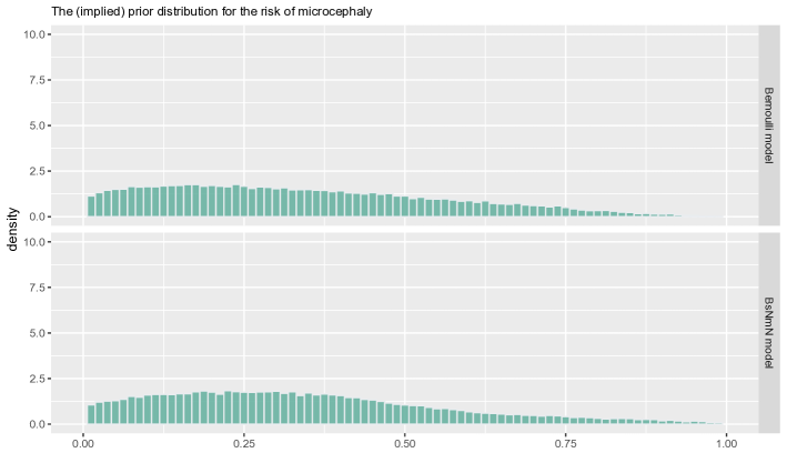
We set a prior for (see top panel of Figure 4), corresponding to an a priori belief that .
We fit the Bernoulli model to the complete case data () and obtained an estimate of: , 95%CrI= [7.84%, 11.39%] (posterior median and equal-tailed 95% credible interval). We also fit the Bernoulli model to the entire dataset (= 1,800) and followed Gelman’s three-step procedure with SVL imputation. Specifically, we used MICE specifying the “logreg” method for and the “normal” method for and . For each of 50 imputed datasets, we fit the Bernoulli model using MCMC with = 5,000 draws and after combining all 250,000 draws together, we obtained an estimate of: , 95%CrI= [11.06%, 14.56%].
The BsNmN model involves a series of conditional distributions for each of the three source variables. We assume that an infant’s sex () is unlikely to impact their gestational age at birth () (at least by any appreciable amount; see Broere-Brown et al. (2016)). Therefore, for sex, we define:
| (5) |
The distribution of gestational age () is known to be skewed with a long left tail (due to preterm delivery), almost complete truncation on the right tail at 45 weeks (due to medically-induced labour at around 45 weeks) and almost complete truncation on the left tail at around 24 weeks (due to viability). Many complex distributions have been suggested for modelling gestational age (e.g., Rathjens et al. (2023) recommends the three-parameter Dagum distribution). Following Sauzet et al. (2015), we choose to define a skew-Normal distribution centered at 39 weeks:
| (6) |
where is the mean of the distribution (known to be approximately 39 weeks, according to Sauzet et al. (2015)), is the scale, and is the slant.
Finally, head circumference () is known to be approximately Gaussian and increases in an approximately quadratic way with gestational age (see Figure 2C in Villar et al. (2014), and Figure 8 in the Appendix). In a ZIKV infected population, infection will cause a certain proportion of infants to have smaller heads. As in Kalmin et al. (2019), we define a Normal mixture distribution for :
| (7) |
where is the proportion of “non-affected” individuals and is the proportion of “affected” individuals. The , , and parameters relate the distribution of head circumference to sex and gestational age for the “non-affected” population; and the and parameters correspond to the impact of ZIKV for the “affected” individuals in terms of the difference in mean head circumference and the scale.
The parameters in the BsNmN model are and each requires a prior. Based on the information available in Villar et al. (2014) and Sauzet et al. (2015), we can be reasonably certain of how gestational age and head circumference are distributed in the non-affected population and therefore set the following informative priors:
| and |
For the scale and slant parameters, we set the following weakly informative priors:
Finally, for the two parameters that define the impact of ZIKV, we set the following priors:
The truncated Normal prior for was chosen in an effort to help address issues with identifiability that are common when fitting Bayesian mixture models; see Betancourt (2017).
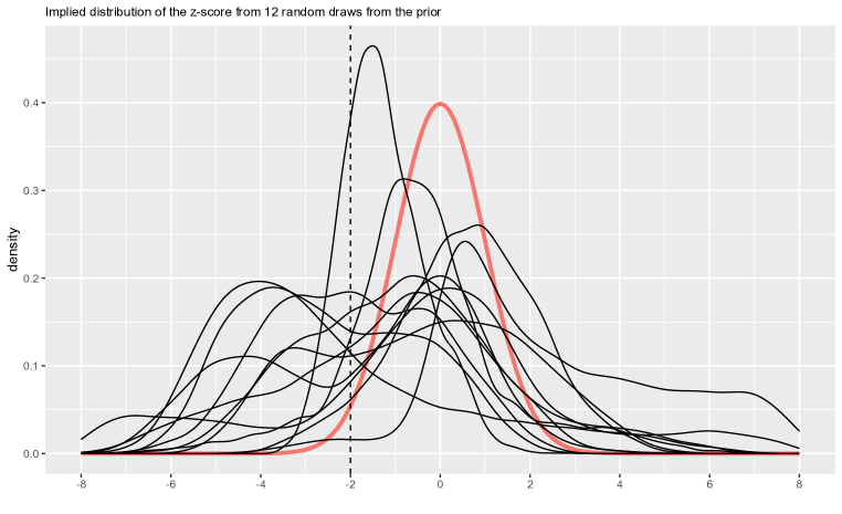
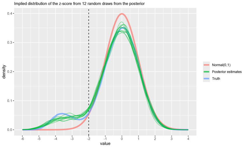
These priors correspond to an a priori belief that . The bottom panel of Figure 4 plots the implied prior distribution for (i.e., for the risk of microcephaly) and Figure 5 plots the implied distribution of the z-score from 12 random draws of the prior.
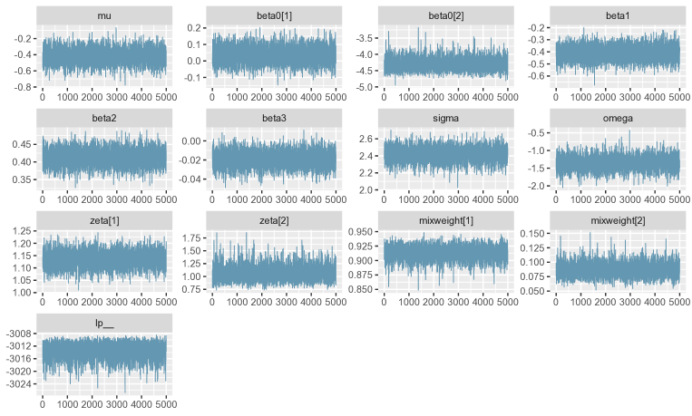
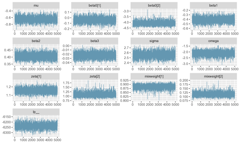
Fitting the BsNmN model to the complete case data () we obtain an estimate of: , 95%CrI= [7.62%, 10.94%]. We also applied the proposed approach to fit the BsNmN model to the entire dataset () as detailed in Section 2 with =5,000 and obtained an estimate of: , 95%CrI= [10.18%, 13.30%]. Figure 6 plots the implied distribution of the z-score from the prior and posterior. Figures 9 and 10 in the Appendix show the trace plots of the MCMC.
| Data | Model | Estimate |
|---|---|---|
| Complete case data () | Bernoulli | , 95%CrI= [7.84%, 11.39%] |
| BsNmN | , 95%CrI= [7.62%, 10.94%] | |
| Entire dataset () | Bernoulli | , 95%CrI= [11.06%, 14.56%] |
| BsNmN | , 95%CrI= [10.18%, 13.30%] |
5 Discussion
The advantages of modelling the source variables directly include the ability to incorporate informed priors specific to the individual source variables and model missingness within a fully Bayesian model following our proposed method. One could also incorporate adjustments for other sources of bias beyond missingness such as preferential sampling (Campbell et al. 2022) and measurement error. This is an important future goal for the microcephaly model given the issues considered by Harville et al. (2020). Including additional variables in the model (e.g., variables that are potentially prognostic factors for microcephaly including exposure to teratogens, and maternal age (Liu et al. 2019)) is another important objective.
There will also be disadvantages to modelling the source variables directly. The additional complexity involved compared to fitting a simpler model involving only the derived variable will likely increase the risk of model misspecification. This includes the risk of misspecifying the priors. Indeed one must be careful to ensure that the “implied” prior on the distribution of the derived variable is reasonable and this is not always obvious (Lockhart 2019). In the microcephaly example, much effort was involved in selecting priors for the BsNmN model such that the implied prior distribution on the risk of microcephaly was reasonable. (The prior for the Bernoulli model was selected in order for the two models to have (implied) priors matching as closely as possible; see Figure 4).
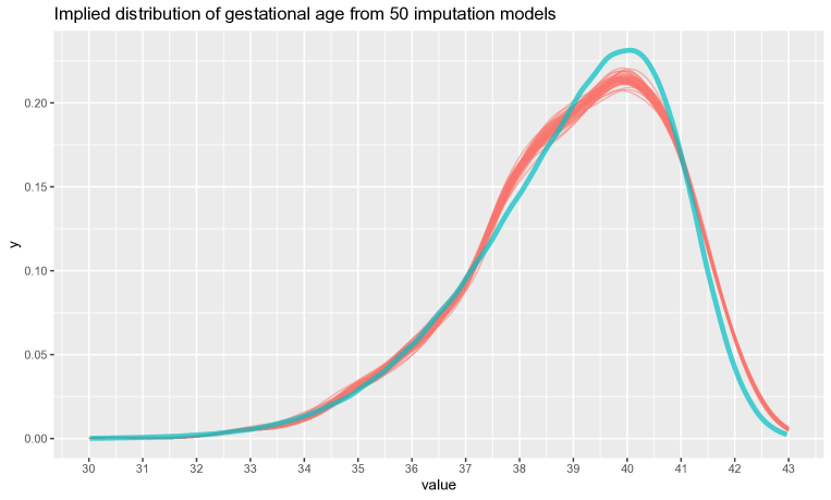
Finally, we note that there is also a risk of model misspecification when using MICE. In the microcephaly example, the Bernoulli model with the entire dataset analysis appears to be biased ( vs the truth ). We suspect that this is due to the distributional assumptions invoked in the MICE algorithm being too simplistic for these data. Specifically, a normal distribution was assumed for missing gestational age values when, in reality, the data are highly skewed. Figure 7 shows how this results in a slight overestimation of the missing values, which, in turn, leads to a relatively large overestimation in the number of microcephaly cases.
References
- (1)
- Bartlett et al. (2015) Bartlett, J. W., Seaman, S. R., White, I. R., Carpenter, J. R. & Alzheimer’s Disease Neuroimaging Initiative* (2015), ‘Multiple imputation of covariates by fully conditional specification: accommodating the substantive model’, Statistical Methods in Medical Research 24(4), 462–487.
- Betancourt (2017) Betancourt, M. (2017), ‘Identifying bayesian mixture models’, Stan Case Studies, mc-stan.org/users/documentation/case-studies/identifying_mixture_models.html .
- Broere-Brown et al. (2016) Broere-Brown, Z. A., Baan, E., Schalekamp-Timmermans, S., Verburg, B. O., Jaddoe, V. W. & Steegers, E. A. (2016), ‘Sex-specific differences in fetal and infant growth patterns: a prospective population-based cohort study’, Biology of Sex Differences 7(1), 1–9.
- Campbell et al. (2022) Campbell, H., de Valpine, P., Maxwell, L., de Jong, V. M., Debray, T. P., Jaenisch, T. & Gustafson, P. (2022), ‘Bayesian adjustment for preferential testing in estimating infection fatality rates, as motivated by the covid-19 pandemic’, The Annals of Applied Statistics 16(1), 436–459.
- Carpenter et al. (2017) Carpenter, B., Gelman, A., Hoffman, M. D., Lee, D., Goodrich, B., Betancourt, M., Brubaker, M. A., Guo, J., Li, P. & Riddell, A. (2017), ‘Stan: A probabilistic programming language’, Journal of Statistical Software 76.
- Erler et al. (2021) Erler, N. S., Rizopoulos, D. & Lesaffre, E. M. E. H. (2021), ‘JointAI: Joint analysis and imputation of incomplete data in R’, Journal of Statistical Software 100(20).
- Gelman et al. (2004) Gelman, A., Carlin, J. B., Stern, H. S., Dunson, D. B., Vehtari, A. & Rubin, D. B. (2004), Bayesian Data Analysis, CRC press.
- Gottschall et al. (2012) Gottschall, A. C., West, S. G. & Enders, C. K. (2012), ‘A comparison of item-level and scale-level multiple imputation for questionnaire batteries’, Multivariate Behavioral Research 47(1), 1–25.
- Harville et al. (2020) Harville, E. W., Buekens, P. M., Cafferata, M. L., Gilboa, S., Tomasso, G. & Tong, V. (2020), ‘Measurement error, microcephaly prevalence and implications for Zika: An analysis of Uruguay perinatal data’, Archives of Disease in Childhood 105(5), 428–432.
- Kalmin et al. (2019) Kalmin, M. M., Gower, E. W., Stringer, E. M., Bowman, N. M., Rogawski McQuade, E. T. & Westreich, D. (2019), ‘Misclassification in defining and diagnosing microcephaly’, Paediatric and Perinatal Epidemiology 33(4), 286–290.
- Liu et al. (2019) Liu, S., … & Chen, D. (2019), ‘Small head circumference at birth: a multiyear liveborn cohort study in china’, BMJ Paediatrics Open .
- Lockhart (2019) Lockhart, R. A. (2019), ‘Bayes factors with (overly) informative priors’, arXiv preprint arXiv:1907.02473 .
- Pan et al. (2020) Pan, Y., He, Y., Song, R., Wang, G. & An, Q. (2020), ‘A passive and inclusive strategy to impute missing values of a composite categorical variable with an application to determine HIV transmission categories’, Annals of Epidemiology 51, 41–47.
- Pham et al. (2021) Pham, T. M., White, I. R., Kahan, B. C., Morris, T. P., Stanworth, S. J. & Forbes, G. (2021), ‘A comparison of methods for analyzing a binary composite endpoint with partially observed components in randomized controlled trials’, Statistics in Medicine 40(29), 6634–6650.
- Rathjens et al. (2023) Rathjens, J., Kolbe, A., Hölzer, J., Ickstadt, K. & Klein, N. (2023), ‘Bivariate analysis of birth weight and gestational age by Bayesian distributional regression with copulas’, Statistics in Biosciences pp. 1–28.
- Reiter & Raghunathan (2007) Reiter, J. P. & Raghunathan, T. E. (2007), ‘The multiple adaptations of multiple imputation’, Journal of the American Statistical Association 102(480), 1462–1471.
- Rubin (1976) Rubin, D. B. (1976), ‘Inference and missing data’, Biometrika 63(3), 581–592.
- Sauzet et al. (2015) Sauzet, O., Ofuya, M. & Peacock, J. L. (2015), ‘Dichotomisation using a distributional approach when the outcome is skewed’, BMC Medical Research Methodology 15, 1–11.
- Van Buuren (2018) Van Buuren, S. (2018), Flexible imputation of missing data, CRC press.
- van Buuren et al. (2015) van Buuren, S., Groothuis-Oudshoorn, K., Robitzsch, A., Vink, G., Doove, L., Jolani, S. et al. (2015), ‘Package ‘mice”, Computer Software .
- Villar et al. (2014) Villar, J., Ismail, L. C., Victora, C. G., Ohuma, E. O., Bertino, E., Altman, D. G., Lambert, A., Papageorghiou, A. T., Carvalho, M., Jaffer, Y. A. et al. (2014), ‘International standards for newborn weight, length, and head circumference by gestational age and sex: the newborn cross-sectional study of the INTERGROWTH-21st Project’, The Lancet 384(9946), 857–868.
- Wilder-Smith et al. (2019) Wilder-Smith, A., Wei, Y., de Araújo, T. V. B., VanKerkhove, M., Martelli, C. M. T., Turchi, M. D., Teixeira, M., Tami, A., Souza, J., Sousa, P. et al. (2019), ‘Understanding the relation between zika virus infection during pregnancy and adverse fetal, infant and child outcomes: a protocol for a systematic review and individual participant data meta-analysis of longitudinal studies of pregnant women and their infants and children’, BMJ Open 9(6), e026092.
- Zhou & Reiter (2010) Zhou, X. & Reiter, J. P. (2010), ‘A note on Bayesian inference after multiple imputation’, The American Statistician 64(2), 159–163.
- Zika Virus Individual Participant Data Consortium (2020) Zika Virus Individual Participant Data Consortium (2020), ‘The Zika virus individual participant data consortium: A global initiative to estimate the effects of exposure to Zika virus during pregnancy on adverse fetal, infant, and child health outcomes’, Tropical Medicine and Infectious Disease 5(4), 152.
6 Appendix
In the simulation study, the three-step approach with JAV (A5) imputation appears to be biased. This is surprising, since in this case the JAV imputation should be identical to the SVL imputation.
Recall that JAV imputation used a fully-conditional specification procedure – specifically the chained equations flavour – rather than a joint model. Denote a random draw with ∗ and the th cycle using the superscript (c). The procedure (typically) initiates in a monotone fashion, visiting variables from least to most missing data, omitting incomplete variables that have not yet been imputed at the zeroth cycle. By construction, always has more missing data than or and, in a given repetition, either or may have the least. For illustration, suppose that has the least missing data. The procedure then draws
So far, this is identical to SVL imputation. Next, the procedure aims to draw
To do so, it starts by fitting a linear regression model for conditioning on (note that are not conditioned-on because chained equations fits the imputation model for a given variable among those with that variable observed, which makes it more efficient than a Gibbs sampler). Now that conditions on the variables that perfectly predict its value, the linear regression model will correctly estimate the coefficients, without uncertainty and without residual error. Even if it draws then and so on, the final imputations have already been completely determined by and . Thus, the procedure should be identical to SVL imputation. Where does the apparent bias come from? We believe it is due to default choices made by the R package mice (possibly to handle perfect prediction, or drop variables; we are unsure). Indeed, to check this, we re-ran the simulation study using Stata’s mi impute chained to perform the imputation and, as expected, found that the JAV procedure described above was unbiased as expected.
6.1 stan code
Bernoulli_model <-
  "data {
  int<lower=0> N;     // Number of observations
  int<lower=0, upper=1> y[N];   // Binary outcome data
  real<lower=0> a;               // Beta distribution shape parameter
  real<lower=0> b;               // Beta distribution shape parameter
}

parameters {
  real<lower=0, upper=1> theta;  // Probability of success
}

model {
  // Likelihood
  for (i in 1:N) {
    y[i] ~ bernoulli(theta);
  }

  // Priors
  theta ~ beta(a, b);
}"


BsNmN_model <- "data {
  int<lower=0> N;
  int<lower=0, upper=N> N_z1obs;
  int<lower=0, upper=N> N_z2obs;
  int<lower=0, upper=N> N_z3obs;
  int<lower=0, upper=N> N_z1mis;
  int<lower=0, upper=N> N_z2mis;
  int<lower=0, upper=N> N_z3mis;
  vector<lower=0, upper=1>[N_z1obs] z1_obs;  // sex variable
  vector[N_z2obs] z2_obs;             // gestational age variable
  vector[N_z3obs]  z3_obs;             // head circumf. variable
  int<lower=0, upper=1> z1mis_ind[N];
  int<lower=0, upper=N> ii_z1_obs[N_z1obs];
  int<lower=0, upper=N> ii_z2_obs[N_z2obs];
  int<lower=0, upper=N> ii_z3_obs[N_z3obs];
  int<lower=0, upper=N> ii_z1_mis[N_z1mis];
  int<lower=0, upper=N> ii_z2_mis[N_z2mis];
  int<lower=0, upper=N> ii_z3_mis[N_z3mis];
}

parameters {
  vector<lower=0, upper=1>[N_z1mis] z1_mis;
  vector[N_z2mis]  z2_mis;
  vector[N_z3mis]  z3_mis;
  real<upper=-1> kappa;
  real beta01;
  vector<lower=0>[2] zeta;
  real beta1;
  real beta2;
  real beta3;
  simplex[2] mixweight;

  real mu; // mean of X
  real<lower=0> sigma; // SD of X
  real omega; // shape of X
}

transformed parameters {
  vector[N] z1;  // sex variable
  vector[N] z2;  // gestational age variable
  vector[N] z3;  // head cir variable
  z1[ii_z1_obs] = z1_obs;
  z1[ii_z1_mis] = z1_mis;
  z2[ii_z2_obs] = z2_obs;
  z2[ii_z2_mis] = z2_mis;
  z3[ii_z3_obs] = z3_obs;
  z3[ii_z3_mis] = z3_mis;
  vector[2] beta0;
  real loc_x; // location of X
  real gm_x; // intermediate calculation for location and scale

  gm_x = sqrt(2/pi())*omega/sqrt(1+omega^2);
  loc_x = mu - sigma*gm_x/sqrt(1-gm_x^2);
  beta0[1] = beta01;
  beta0[2] = kappa;
}

model {
  // Prior distributions for GA
  mu ~ normal(0, 0.1);
  sigma ~ inv_gamma(2, 2);
  omega ~ normal(0, 2);

  // Prior distributions for HC:
  beta0[1] ~ normal(0, 0.1);
  beta0[2] ~ normal(-2, 2)T[,-1];
  zeta[1] ~ inv_gamma(2, 2);
  zeta[2] ~ inv_gamma(2, 2);
  beta1 ~ normal(-0.450, 0.1);
  beta2 ~ normal(0.399, 0.1);
  beta3 ~ normal(-0.016, 0.1);

  // Likelihood
 z1_mis ~ uniform(0,1);

 z2_obs ~ skew_normal(loc_x, sigma, omega);
 z2_mis ~ skew_normal(loc_x, sigma, omega);

 vector[2] log_mixweight = log(mixweight);
 for (n in 1:N) {
 Ψvector[2] lps = log_mixweight;
// for unknown sex
   if (z1mis_ind[n]==1 ) {
ΨΨ    for (k in 1:2) {
 ΨΨΨΨlps[k] += log_mix( z1[n],
                    normal_lpdf( z3[n] | 33.912 + beta0[k] + beta1 + beta2*z2[n] +
                    beta3*pow(z2[n],2), zeta[k]),
                    normal_lpdf( z3[n] | 33.912 + beta0[k]  + beta2*z2[n]+
                    beta3*pow(z2[n],2), zeta[k]));
    ΨΨ}Ψ    ΨΨ
  Ψ}
// for known sex  Ψ
Ψelse {
ΨΨΨfor (k in 1:2) {
ΨΨ      lps[k] += normal_lpdf(z3[n] | 33.912 + beta0[k] +
ΨΨ      Ψbeta1*z1[n] + beta2*z2[n]+
                    beta3*pow(z2[n],2), zeta[k]);
    ΨΨ}  Ψ Ψ
  Ψ}
  Ψtarget += log_sum_exp(lps);
  }
}
"