Invariant Subspace Decomposition
Abstract
We consider the task of predicting a response from a set of covariates in settings where the conditional distribution of given changes over time. For this to be feasible, assumptions on how the conditional distribution changes over time are required. Existing approaches assume, for example, that changes occur smoothly over time so that short-term prediction using only the recent past becomes feasible. In this work, we propose a novel invariance-based framework for linear conditionals, called Invariant Subspace Decomposition (ISD), that splits the conditional distribution into a time-invariant and a residual time-dependent component. As we show, this decomposition can be utilized both for zero-shot and time-adaptation prediction tasks, that is, settings where either no or a small amount of training data is available at the time points we want to predict at, respectively. We propose a practical estimation procedure, which automatically infers the decomposition using tools from approximate joint matrix diagonalization. Furthermore, we provide finite sample guarantees for the proposed estimator and demonstrate empirically that it indeed improves on approaches that do not use the additional invariant structure.
1 Introduction
Many commonly studied systems evolve with time, giving rise to heterogeneous data. Indeed, changes over time in the data generating process are reflected by shifts in the data distribution, and make it in general impossible to find a fixed model that consistently describes the system through time. In regression settings, varying-coefficients models (e.g., Hastie and Tibshirani, 1993; Fan and Zhang, 2008) are a common approach to deal with dynamic system behaviours related to changes in the functional relationship between a response and some covariates. Another approach for online estimation of changing parameters uses state-space models and filtering solutions (see, for example, Durbin and Koopman, 2012). Changes in time of the covariates distribution can instead be modeled, for example, as non-stationarity in time-series.
In this work, we analyze the problem of estimating the relation between a response and a set of covariates (or predictors) , , that are observed over some period of time, with the goal of short term prediction of an unobserved response, when the observations of new covariates become available. Changes in the data distribution can occur, for example, if the mechanism relating the response to the covariates or the covariates distribution vary with time : in our setting, we allow for both such changes to happen. The task of predicting an unobserved response is then only feasible if some information from past time points can be used. This, in general, requires assumptions on how the underlying data generating model changes over time. For example, if changes happen smoothly, then the most relevant observations are likely the last available. To also exploit information further in the past, it is sometimes of interest to look for invariant patterns that persist through time. In this spirit, Meinshausen and Bühlmann (2015) define the maximin effect as a worst case optimal model that maintains good predictive properties at all observed times. Invariance based methods are also used in the machine learning literature to deal with covariates shifts. One relevant example is unsupervised domain adaptation (see, for example, Sun et al., 2017; Zhao et al., 2019; Stojanov et al., 2021), which aims at transferring invariant information from a source domain to a target domain in which the response is not observed. The concept of invariance is widely explored in the field of causal inference, too. In causal models, changes in the covariates distribution are modeled as interventions, and different interventional settings represent different environments. In this context, Peters et al. (2016) propose to look for a set of stable causal predictors, that is, a set of covariates for which the conditional distribution of the response given such covariates remains invariant across different environments. The same idea is extended by Pfister et al. (2019a) to a sequential setting in which the different environments are implicitly generated by changes of the covariates distribution over time. Such invariances can then be used for prediction in previously unseen environments, too (e.g., Rojas-Carulla et al., 2018; Magliacane et al., 2018; Pfister et al., 2021).
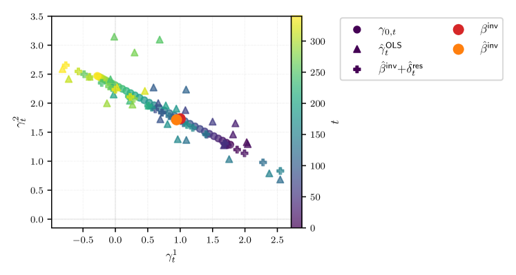
In this work, we build on this invariance idea and exploit it for time adaptation: we propose an invariance based framework, which we call invariant subspace decomposition (ISD), for the estimation of time-varying regression models. More in detail, we aim at finding the time-varying functional relationship between the covariates and the response through the maximization of the explained variance at time , which is given for some function by . The explained variance constitutes an objective function equivalent to the mean squared error (with opposite optimization sign), and has the advantage of providing an intuitive evaluation of the predictive quality of a function : negative explained variance indicates in particular that using for prediction is harmful, in that it is worse than using the zero function. We study the case in which is a linear function. Key to ISD is the decomposition of the explained variance maximization into a time-invariant and a time-dependent part. To achieve the decomposition, we exploit ideas from independent subspace analysis (see, for example, the work by Gutch and Theis, 2012) and seek a transformation of the original space (in which the covariates are observed), such that the number of pairwise uncorrelated components of the transformed covariates is maximized at all observed time points. The key aspect of such a decomposition is that it allows us to look at two sub-problems, each of which has less degrees of freedom than the original one: (i) an invariant problem that can be solved only once exploiting all available heterogeneous data and (ii) an adaptation problem that tunes the invariant solution to a time-point of interest. This result is summarized in Theorem 1. The solution to (i) is a time-invariant linear parameter () that partially describes the data at all times and, in lack of reliable data to solve the time-adaptation step, can be used for zero-shot prediction. The solution to (ii) () can be seen as a fine-tuning of the solution to (i) to learn the time-varying linear parameter of interest (). A simple -dimensional example is shown in Figure 1 and later presented in Example LABEL:ex:running_ex_2d: here, the true time-varying linear parameter varies in a one dimensional subspace of , while the time-invariant parameter lies in the corresponding orthogonal subspace. Moreover, the components of the covariates along these two orthogonal subspaces are uncorrelated.
The fundamental assumption we make for ISD is that the decomposition inferred from available observations generalizes to unseen time points. The main implication of such generalization assumption is that, once an estimate of the invariant component that solves step (i) is available, it can, at all new time points, either be used directly for prediction or as part of a two-step estimation that is fine-tuned with step (ii), which only solves the time adaptation part of the problem.
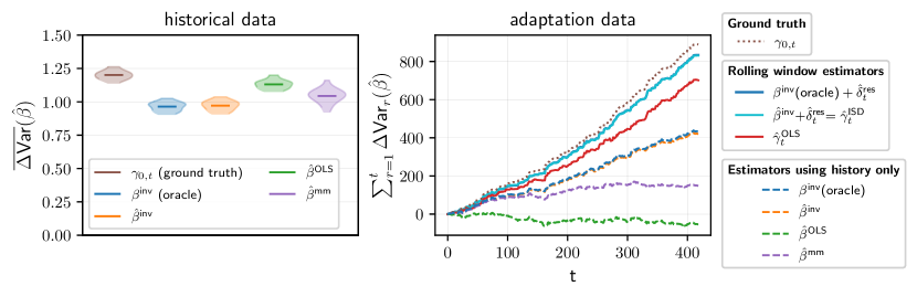
Figure 2 shows the cumulative explained variance by the invariant component and the adapted invariant component estimated in a simulated setting at training time (left) within the observed time horizon, and at testing time (right) when new observations become available. We compare the ISD with the standard OLS solution, computed both on all training observations and on a rolling window over the latest new observations, and with the maximin effect () by Meinshausen and Bühlmann (2015), which maximizes the worst case explained variance over the available observations.
The remainder of the paper is structured as follows. In Section 2 we introduce the ISD framework for orthogonal transformations. We then describe, in Section 3, the two tasks that ISD solves, namely zero-shot prediction and time-adaptation. In Section 4 we propose an estimation method for ISD, and provide finite sample generalization guarantees for the proposed estimator. Finally, in Section 5, we illustrate ISD based on numerical experiments and validate the theoretical results presented in the paper.
2 Invariant subspace decomposition
Let be a sequence of independent random vectors satisfying for all a linear model of the form
| (1) |
where is the (unknown) true time-varying parameter. We further assume that for all the covariance matrix of the predictors is strictly positive definite. Moreover, for all we define the set .
We are interested in predicting the response from the observed data and the predictor in settings where the true time-varying parameter is constant or approximately constant only in short periods of time, e.g., step-wise constant (we refer to the case as zero-shot generalization; is a special case of what we refer to as time-adaptation, see Section 3). A naive solution is to only consider the most recent observations, assuming that the model is approximately time-invariant over these observations. Our goal in this work is to improve on this approach and exploit all observations in . To achieve this, we propose to learn two parameters whose sum equals the time-varying parameter : a time-invariant parameter , defined formally below in Section 2.2, and an adaptation parameter defined formally in Section 2.3 that explains the remaining residuals . The separation allows us to first use all available observations in to estimate the time-invariant parameter, and to then improve the prediction (using only the most recent observations) by learning an adaptation parameter with less degrees of freedom, explaining the remaining variance.
Before we define time-invariant parameters, we first consider the explained variance for a parameter at time , defined by
Under model (1), the explained variance can be equivalently expressed as
| (2) |
The true time-varying parameter can always be expressed as
| (3) |
A desirable property for a non-varying parameter is to guarantee that its explained variance remains non-negative at all time points. We call parameters never harmful if, for all , . Intuitively, parameters with this property at least partially explain at all time points , and are therefore meaningful to use for prediction.111Under an assumption similar to Assumption 2 below, the maximin framework by Meinshausen and Bühlmann (2015) allows us to estimate never harmful parameters: we provide a more detailed comparison between our approach and the maximin in Remark 2. In this paper, we consider the subset of never harmful parameters that satisfy or equivalently, using (2), ; thus, the explained variance of these parameters reflects changes of (over ) but is independent of changes in .
Definition 1 (time-invariance).
We call a parameter time-invariant (over ) if for all ,
| (4) |
We show in Theorem 1 that, under some additional assumptions, the true time-varying parameter can be decomposed into a time-invariant component and a time-varying component ; furthermore, this decomposition can be obtained by splitting the parameter space into two orthogonal linear subspaces with such that, for all ,
| (5) |
where . Thus, we can view as splitting the optimization into two parts: (i) a time-invariant part that optimizes the pooled explained variance over , leveraging all observations in , and (ii) a residual part that optimizes the explained variance at a single time point over a (potentially) lower dimensional linear space . The linear space does not only contain time-invariant parameters. However, as we show in Proposition 2, the parameter maximizing the pooled explained variance over is always a time-invariant parameter.
In this work, we consider explained variance as an objective. Equivalently, one can consider the mean squared prediction error (MSPE).
Remark 1 (Exchanging explained variance with MSPE).
Under model (1) maximizing the explained variance at time is equivalent to minimizing the MSPE at , . More precisely, assuming that all variables have mean zero,
The remaining part of this section is organized as follows. Section 2.1 explicitly constructs the spaces and and shows that they can be characterized by joint block diagonalization. In Section 2.2 we then analyze the time-invariant part of (5), leading to the optimal time-invariant parameter , and show in Proposition 2 that its solution corresponds to the maximally predictive time-invariant parameter and is an interesting target of inference in its own right. In Section 2.3 we analyze the residual part of (5), leading to the optimal parameter .
2.1 Invariant and residual subspaces
We now construct the two linear subspaces and that allow us to express the true time-varying parameter as the solution to two separate optimizations as in (5). For a linear subspace , denote by the orthogonal projection matrix from onto . We call a collection of pairwise orthogonal linear subspaces with an orthogonal partition w.r.t. (of cardinality ) if for all with , and for all it holds that
| (6) |
Moreover, we call an orthogonal partition w.r.t. irreducible if there is no other orthogonal partition w.r.t. with strictly larger cardinality.
For an orthogonal (not necessarily irreducible) partition w.r.t. we show in Lemma 3 that
| (7) |
where denotes the Moore-Penrose pseudoinverse. A direct computation (see Lemma 4) further shows that, for all and all ,
| (8) |
where to show that the argmax is unique we used that is invertible by assumption. Combining (7) and (8) implies that
Therefore, any orthogonal partition w.r.t. allows to split the optimization (3) of the explained variance into separate optimizations over the individual subspaces. In order to leverage all available observations in at least some of the optimizations by pooling the explained variance as in (5), we need the optimizer to remain constant over time. More formally, we call a linear subspace opt-invariant on if for all it holds that
| (9) |
namely the optimizer of over remains invariant across . For an irreducible orthogonal partition , we now define the invariant subspace and the residual subspace by
| (10) |
respectively. The invariant subspace is opt-invariant (see Lemma 5). Moreover, by definition, it holds that , where denotes the orthogonal complement in , and that is an orthogonal partition w.r.t. (see Lemma 6). To ensure that these two spaces do not depend on the chosen irreducible subspace partition we introduce the following assumption.
Assumption 1 (uniqueness of the subspace decomposition).
Let and be two irreducible orthogonal partitions w.r.t. . Then, it holds that
Assumption 1 is for example satisfied if an irreducible orthogonal partition w.r.t. is unique but, as we show in Appendix A.1, such uniqueness does not necessarily hold and, furthermore, Assumption 1 may be violated. Assumption 1 is, however, a mild assumption; for example, the uniqueness of an irreducible orthogonal partition w.r.t. is satisfied if there exists at least one such that all eigenvalues of , which we have assumed to be non-zero, are distinct (see Lemma 7 and Proposition 1 below). Whenever Assumption 1 holds, the invariant and residual spaces and do not depend on which irreducible orthogonal partition is used in their construction.
Example 1 (label=ex:running_ex_2d).
This example describes the setting used to generate Figure 1. Consider a -dimensional covariate , and assume that model (1) is defined as follows. We take, for all
where and are two fixed sequences sampled as two independent i.i.d. samples from a uniform distribution on . In this example, we have that an irreducible orthogonal partition is given by the two spaces
Indeed, it holds for all that . Moreover, since and are the eigenvalues of , the irreducible orthogonal partition defined by and is unique (i.e., Assumption 1 is satisfied by Lemma 7) if for some . It also holds that
which does not depend on (it can be verified that the same does not hold for ). As can be seen from the proof of Proposition 2 (i) below, it holds that
It follows that the subspace is opt-invariant, whereas is not, and therefore and . The two spaces and also appear in Figure 1: the true time-varying parameter does not vary with in the direction of the vector generating ; can be visualized when connecting the circles.
In order for and to be useful for prediction on future observations, we assume that the subspace separations we consider remain fixed over time.
Assumption 2 (generalization).
For all irreducible orthogonal partitions w.r.t. , and defined in (10) satisfy the following two conditions: (i) for all it holds that and (ii) is opt-invariant on .
As shown in the following theorem, Assumption 2 ensures that the two sets satisfy a separation of the form (5) as desired. For unobserved time points , Assumption 2 does not require (6) to hold for all , but only for all such that and .
Theorem 1.
Assume Assumption 2 is satisfied. Let and be defined as in (10) for an arbitrary irreducible orthogonal partition w.r.t. . Then, it holds for all that
| (11) |
where . Moreover, if Assumption 1 is satisfied, the separation in (11) is independent of the considered irreducible orthogonal partition w.r.t. .
2.1.1 Identifying invariant and residual subspaces using joint block diagonalization
We can characterize an irreducible orthogonal partition using joint block diagonalization of the set of covariance matrices . Joint block diagonalization of consists of finding an orthogonal matrix such that the matrices , , are block diagonal and we can choose blocks such that the indices of the corresponding submatrices do not change with (the entries of the blocks may change with though). Let be the largest number of such blocks and let denote the corresponding common blocks with dimensions that are independent of . We call a joint block diagonalizer of . Moreover, we call an irreducible joint block diagonalizer if, in addition, for all other joint block diagonalizers the resulting number of common blocks is at most . Joint block diagonalization has been considered extensively in the literature (see, for example, Murota et al., 2010; Nion, 2011; Tichavsky and Koldovsky, 2012) and various computationally feasible algorithms have been proposed (see Section A.3 for further details).
In our setting, joint block diagonalization can be used to identify the invariant and residual subspaces, since an irreducible joint block diagonalizer of the covariance matrices corresponds to an irreducible orthogonal partition, as the following proposition shows.
Proposition 1.
Let be an irreducible joint block diagonalizer of . For all , let denote the subset of indices corresponding to the -th common block . Moreover, let denote the -th column of and, for all , define
Then, is an irreducible orthogonal partition w.r.t. .
The reverse of Proposition 1 is true as well, as shown in Lemma 2. From Proposition 1 it also follows for all that the orthogonal projection matrix onto the subspace can be expressed as , where we denote by the submatrix of formed by the columns indexed by . Moreover, if Assumption 1 is satisfied, any irreducible joint block diagonalizer , via its corresponding irreducible orthogonal partition w.r.t. constructed in Proposition 1, leads to the same (unique) invariant and residual subspaces defined in (10).
It is clear that Assumption 1 is automatically satisfied whenever the joint block diagonalization is unique up to trivial indeterminacies, that is, if for all orthogonal matrices that jointly block diagonalize the set into irreducible common blocks, it holds that is equal to up to block permutations and block-wise isometric transformations. Explicit conditions under which uniqueness of joint block diagonalization is satisfied can be found, for example, in the works by De Lathauwer (2008); Murota et al. (2010).
Given an irreducible joint block diagonalizer , the invariant and residual subspaces can be identified using Proposition 1 and Lemma 4, by checking for all whether remains constant () or not () on . We denote by and the submatrices of formed by the columns that span the invariant and the residual subspace respectively.
Example 2 (continues=ex:running_ex_2d).
In Example 1 so far, we expressed and in terms of their generating vectors. These can be retrieved using Proposition 1 by joint block diagonalizing the matrices . In this specific example, an irreducible joint block diagonalizer is given by
which is a (clockwise) rotation matrix of degrees (see Figure 1 and use and ). In particular, we have that : therefore, and each block has dimension . Moreover, it holds for all that
and therefore and .
2.2 Invariant component
In Theorem 1 we have shown that the true time-varying parameter can be expressed as the result of two separate optimization problems over the two orthogonal spaces and . In this section we analyze the result of the first optimization step over the invariant subspace . To ensure that the space is unique, we assume that Assumption 1 is satisfied throughout Section 2.2.
Definition 2 (Invariant component).
We denote the parameter that maximizes the explained variance over the invariant subspace by
| (12) |
The parameter corresponds to the pooled OLS solution obtained by regressing on the projected predictors , and can be computed using all observations in . The procedure to find by first identifying via joint block diagonalization and then using Proposition 2 below is later summarized in Algorithm 1; the last step (line ) is based on Definition 2, (7) and (8). Proposition 2 summarizes some of the properties of .
Proposition 2 (Properties of ).
Definition 1 guarantees, for all , that the explained variance for all time-invariant over is . Point of Proposition 2 therefore implies that, for all , . Under Assumption 2, we have that the same holds for all : is therefore a never harmful parameter and for all it is a solution to . Moreover, Proposition 2 implies that, under an additional assumption, the parameter is optimal, i.e., maximizes the explained variance, among all time-invariant parameters. In particular, represents an interesting target of inference: it can be used for zero-shot prediction, if no adaptation data is available at time to solve the second part of the optimization in (11) over . Using as defined in Section 2.1.1, we can express as follows.
| (13) |
where and . We derive this expression in Lemma 9, and we later use it for estimation in Section 4.2.
Example 3 (continues=ex:running_ex_2d).
Considering again Example LABEL:ex:running_ex_2d, we have that , and therefore the invariant component is given by
Moreover, we can express under the basis for the irreducible subspaces using the irreducible joint block diagonalizer , obtaining : the only non-zero component is indeed the one corresponding to the invariant subspace .
2.3 Residual component and time adaptation
Under the generalization assumption (Assumption 2), Theorem 1 implies that we can partially explain the variance of the response at all—observed and unobserved—time points using . It also implies that for all we can reconstruct the true time-varying parameter by adding to a residual parameter that maximizes the explained variance at time over the residual subspace , i.e.,
In this section we focus on the second optimization step over . We assume that Assumptions 1 and 2 hold, and for all we define the residual component Using (7), (8) and (10), we can express as
| (14) | ||||
We can now reduce the number of parameters that need to be estimated by expressing as an OLS solution with parameters. To see this, we use that, under Assumption 1, Proposition 1 allows us to express the space in terms of an irreducible joint block diagonalizer corresponding to the irreducible orthogonal partition as
Moreover, the orthogonal projection matrix onto is given by . Hence, using Lemma 3 we get that
| (15) |
where is the population ordinary least squares solution obtained by regressing on .
Example 4 (continues=ex:running_ex_2d).
In Example 1, we have that for all the residual component is given by
Moreover, we can express under the irreducible orthogonal partition basis (given by the two vectors generating and ), obtaining , which indeed only has one degree of freedom in the first component. This component takes the following values: for all we have .
2.4 Population ISD algorithm
We call the procedure to identify and invariant subspace decomposition (ISD). By construction, the result of ISD in its population version is equal to the true time-varying parameter at time , i.e.,
| (16) |
The full ISD procedure is summarized in Algorithm 1. In the algorithm, the invariant and residual subspaces are identified as described at the end of Section 2.1.1. If Assumption 1 is not satisfied, then the decomposition in (16) and therefore the output of Algorithm 1 depends on the irreducible orthogonal partition w.r.t. used.
In Appendix B we show that a decomposition of the true time-varying parameter similar to (16) is also obtained when considering partitions w.r.t. that are not orthogonal, i.e., such that (6) holds but the subspaces in the partition are not necessarily pairwise orthogonal. In this case, in particular, we can still find an invariant and residual parameter as in (13) and (15), respectively, where the matrix is now a non-orthogonal irreducible joint block diagonalizer.
3 ISD tasks: Zero-shot generalization and time adaptation
We now formally introduce the two tasks that can be solved with the ISD framework introduced in the previous section. Assume we observe observations from model (1), which we call historical data. Furthermore, assume we observe a second set of observations from the same model but succeeding the historical data, which we call adaptation data. Formally, we assume the adaptation window is an interval of consecutive time points with and . Finally, denote by a time point of interest that occurs after the adaptation data and assume that for all , the quantities , and in model (1) are constant (in practice, being approximately constant is sufficient).
Our goal is now to predict from . We distinguish two possible prediction tasks: (i) the zero-shot task, in which we assume that we only have access to the historical data and (ii) the adaptation task, in which we assume that we additionally have access to the adaptation data. The full setup including the different tasks is visualized in Figure 3. Throughout the remainder of this section we assume that the invariant and residual subspaces are known (they can be computed from the joint distributions), which simplifies the theoretical analysis.
3.1 Zero-shot task
We start by analyzing the zero-shot task, in which no adaptation data are observed, but only historical data and . Under the generalization assumption (Assumption 2), is opt-invariant on and we can characterize all possible models defined as in (1) by the possible variations of the true time-varying parameter in the residual space , or, equivalently, by all possible values of . We then obtain that is worst case optimal in the following sense.
We further obtain from Proposition 2 that, under an additional condition, is worst case optimal among all time-invariant parameters. This characterization of allows for a direct comparison with the maximin effect by Meinshausen and Bühlmann (2015), which we report in more detail in Remark 2. In absence of further information on , Theorem 2 suggests to use an estimate of of to predict , i.e., .
Remark 2 (Relation to maximin).
The maximin framework introduced by Meinshausen and Bühlmann (2015) considers a linear regression model with varying coefficients, where the variations do not necessarily happen in a structured way, e.g., in time. Translated to our notation and restricting to time-based changes, their model can be expressed for as
where and the covariance matrix does not vary with . The maximin estimator maximizes the explained variance in the worst (most adversarial) scenario that is covered in the training data; it is defined as
The maximin estimator guarantees that, for all , and therefore (see Meinshausen and Bühlmann, 2015, Equation (8)). This means that the maximin relies on a weaker notion of invariance that only requires the left-hand side of (4) to be non-negative instead of zero. This implies that is in general more conservative than in the sense that, for all , By finding the invariant and residual subspaces, we determine the domain in which varies and assume (Assumption 2) that this does not change even at unobserved time points. The parameter is then worst case optimal over this domain, and guarantees that the explained variance remains positive even for scenarios that are more adversarial than the ones observed in , i.e., such that for some (see, for example, the results of the experiment described in Section 5.1 and shown in Figure 2). Furthermore, the decomposition allows for time adaptation (see Section 2.3), which would not be possible starting from the maximin effect.
3.2 Adaptation task
We now consider the adaptation task in which, additionally to the historical data, adaptation data are available. Adaptation data can be used to define an estimator for the residual component , which we denote by . This, together with an estimator for fitted on the historical data gives us an estimator for the true time-varying parameter. We compare this estimator with a generic estimator for which uses only the adaptation data.
To do so, we consider the minimax lower bound provided by Mourtada (2022)[Theorem 1] for the expected squared prediction error of an estimator computed using i.i.d. observations of a random covariate vector and of the corresponding response . It is given by
| (17) |
where is the class of distributions over such that , and . It follows from (17) that, for a generic estimator of based on the adaptation data alone, we can expect at best to achieve a prediction error of , where is the variance of for (which is assumed to be constant). We can improve on this if we allow the estimator to also depend on the historical data. To see this, observe that we can always decompose with and . Moreover, under Assumption 2 we can split the expected prediction error of at accordingly as
Then, represents an estimator for and can be computed on historical data222In principle, an estimator for could be computed using both historical and adaptation data. However, the ISD procedure is motivated by scenarios in which the size of historical data is very large (and ): this means that it could be computationally costly to update the estimate for the invariant component every time new adaptation data are available, without a significant gain in estimation accuracy. For this reason, we only consider estimators for that use historical data., whereas estimates and is based on adaptation data: by decomposing in this way, the best prediction error we can hope for is of the order . In Section 4, we prove that indeed achieves this bound in Theorem 3. If the invariant subspace is non-degenerate and therefore , and is sufficiently large, this implies that has better finite sample performance than estimators based on the adaptation data alone.
4 ISD estimator and its finite sample generalization guarantee
We now construct an empirical estimation procedure for the ISD framework, based on the results of Section 2.2 and on Algorithm 1 described in Section 2.3. Throughout this section, we assume that Assumptions 1 and 2 are satisfied.
We assume that we observe both historical and adaptation data as in the adaptation task. We use the historical data to first estimate the decomposition of into and , employing a joint block diagonalization algorithm (Section 4.1). We then use the resulting decomposition to estimate . Finally, we use the adaptation data to construct an estimator for in Section 4.2. In Section 4.3 we then show the advantage of separating the optimization as in (5) to estimate at the previously unobserved time point , by providing finite sample guarantees for the ISD estimator.
4.1 Estimating the subspace decomposition
4.1.1 Approximate joint block diagonalization
We first need to find a good estimator for the covariance matrices . Since only one observation is available at each time step , some further assumptions are needed about how varies over time. Here, we assume that varies smoothly with and is therefore approximately constant in small time windows. We can then consider a rolling window approach, i.e., consider windows in of length over which the constant approximation is deemed valid, and for the -th time window, , take the sample covariance as an estimator for in such time window.
Given the set of estimated covariance matrices , we now need to estimate an orthogonal transformation that approximately joint block diagonalizes them. We provide an overview of joint block diagonalization methods in Section A.3 in the appendix. In our simulated settings, we solve the approximate joint block diagonalization (AJBD) problem via approximate joint diagonalization (AJD), since we found this approach to represent a good trade off between computational complexity and accuracy. More in detail, similarly to what is proposed by Tichavsky and Koldovsky (2012), we start from the output matrix of the uwedge algorithm by Tichavsky and Yeredor (2008), which solves AJD for the set , i.e., it is such that for all the matrix is approximately diagonal. We then use the off-diagonal elements of the approximately diagonalized covariance matrices to identify the common diagonal blocks. As described more in detail in Section A.3, this is achieved by finding an appropriate permutation matrix for the columns of such that for all the matrix is approximately joint block diagonal. The estimated irreducible joint block diagonalizer is then given by . We denote by the number of estimated diagonal blocks and by the estimated irreducible orthogonal partition w.r.t. .
4.1.2 Estimating the invariant and residual subspaces
We now estimate the invariant and residual subspaces using the estimated irreducible joint block diagonalizer . To do so, we first estimate the true time-varying parameter using similar considerations as the ones made in Section 4.1.1. We assume for example that is approximately constant in small windows (for simplicity, we consider the same windows defined in Section 4.1.1). We then compute the regression coefficient of on , where and are the observations in the -th time window. We have so far omitted the intercept in our linear model. This can always be included by adding a constant term to and increasing by one the dimension of , adding a row and column at the same index of the constant term, with the off-diagonal entries set to zero and the diagonal entry set to one.
We now use the estimates to determine which of the subspaces identified by are opt-invariant. For all , we take the sets of indices as defined in Proposition 1, and consider the estimated orthogonal projection matrices from onto the -th subspace of the estimated irreducible orthogonal partition. It follows from the proof of Proposition 2 that we can find the opt-invariant subspaces by checking for all whether remains approximately constant for .
We further use that, by Lemma 8, if is opt-invariant on then the (approximately constant) projected regression coefficient approximately satisfies the time-invariance constraint (4). This approach is motivated by Proposition 2 . If the corresponding assumption cannot be assumed to hold, other methods can alternatively be used to determine whether is constant, e.g., checking its gradient or variance. In (4), we can equivalently consider the correlation in place of the covariance, that is, : an estimate of this correlation allows us to obtain a normalized measure of (4) that is comparable across different experiments. Formally, we consider
and check, for all , whether
| (18) |
for some small threshold . The threshold can be chosen, for example, using cross-validation (more details are provided in Section A.2 in the appendix). An estimator of the invariant and residual subspaces is then given by
| (19) |
4.2 Estimating the invariant and residual components
Let and be the submatrices of whose columns span and , respectively. We propose to estimate using the following plug-in estimator for (13)
| (20) |
We consider now the new observation of the covariates at time and the adaptation data introduced in Section 3, and denote by and the matrices containing this adaptation data. Similarly to , using (15) we obtain the following plug-in estimator for
| (21) |
We can now define the ISD estimator for the true time-varying parameter at as
| (22) |
A prediction of the response is then given by .
Example 5 (continues=ex:running_ex_2d).
Assume that in Example 1 the true time-varying parameter at time points is given by
for some . We can verify that , and therefore the invariant and residual subspaces defined on generalize to and Assumption 2 is satisfied. Moreover, we obtain that for the residual component expressed under the irreducible orthogonal partition basis is
The first entry now takes values in , which is disjoint from the range of values of the first coordinate observed in (which was ).
We now take and consider an online setup in which we sequentially observe at a new time point , and assume that is observed until . We take as historical data the observations on , and consider as adaptation data the observations in windows of length . After estimating on historical data, we use the adaptation data to estimate and the OLS solution . We repeat this online step times (each time increasing by one). Figure 1 shows the results of this experiment.
4.3 Finite sample generalization guarantee
Considering the setting described in Section 2.3, we now compare the ISD estimator in (22) with the OLS estimator computed on , i.e., . We assume that we are given the (oracle) subspaces and , and consider the expected explained variance at of and . More in detail, the expected explained variance at of an arbitrary estimator of is given by
| (23) |
Evaluating (23) allows us to obtain a measure of the prediction accuracy of : the higher the expected explained variance, the more predictive the estimator is. This also becomes clear by isolating in (23) the term , which represents the mean square prediction error obtained by using (see Remark 1). Our goal is to show that the explained variance by is always greater than that of the OLS estimator.
Theorem 3.
Assume Assumption 2 and that, in model (1), and the variances of and do not change with respect to , and denote them by , and , respectively. Moreover, let be constants such that for all it holds that and for all with , almost surely, where denotes the smallest eigenvalue. Further assume that the invariant and residual subspaces and are known. Then, there exist constants such that for all with it holds that
Furthermore, for all with it holds that
From the proof of Theorem 3 it follows that can be chosen close to if we only consider sufficiently large . Moreover, because , Theorem 3 implies that if and sufficiently large then
The first term in the difference between the expected explained variances (or MSPEs) depends on the dimensions of the invariant subspace and of the time-adaptation window : there is a higher gain in using instead of if the dimension of is large and only a small amount of time-points are available are available in the adaptation data.
5 Simulation experiments
To show the effectiveness of the ISD framework we report the results of two simulation experiments. The first evaluates the estimation accuracy of the invariant component for increasing sample size of the historical data. The second experiment compares the predictive accuracy of and for different sizes of the adaptation dataset, to empirically investigate the dependence of the MSPE difference on the size of the adaptation data shown in Theorem 3.
In both experiments we let the dimension of the covariates be , and , , and generate data as follows. We sample a random orthogonal matrix , and sample the covariates from a normal distribution with zero mean and covariance matrix , where is a block-diagonal matrix with four blocks of dimensions and , and random entries that change times in the observed time horizon . We take as true time-varying parameter the rotation by of the parameter with constant entries equal to (we set these entries all to the same value for simplicity, but they need not to be equal in general) corresponding to the blocks of sizes and , and time-varying entries—corresponding to the blocks of sizes and —equal to , where is the entry index (the values of these coefficients range between and ). The noise terms are sampled i.i.d. from a normal distribution with zero mean and variance . The code for the presented experiments is available at https://github.com/mlazzaretto/Invariant-Subspace-Decomposition. The implementation of the uwedge algorithm is taken from the Python package https://github.com/sweichwald/coroICA-python developed by Pfister et al. (2019b).
5.1 Invariant decomposition and zero-shot prediction
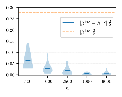
We first estimate the time invariant parameter for different sample sizes of the historical data. We consider , and repeat the experiment times for each . To compute , we use equally distributed windows of length (see Section 4). Figure 4 shows that the mean squared error (MSE) converges to zero for increasing values of .
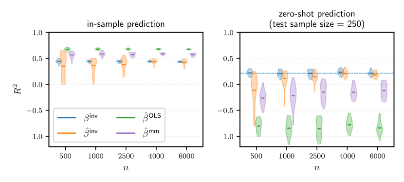
We then consider a separate time window of observations in which the value of the time-varying coefficients (before the transformation using ) is set to . We use these observations to test the zero-shot predictive capability of the estimated invariant component, i.e., they can be seen as realizations of the variable introduced in Section 3 (with a slight abuse of notation, we also refer to this window as adaptation data even though we do not perform the adaptation step). We compare the predictive performance of the parameter on the historical and adaptation data with that of the oracle invariant parameter , the maximin effect (computed using the magging estimator proposed by Bühlmann and Meinshausen, 2015), and the OLS solution , both computed using the historical data. We show in Figure 5 the results in terms of the coefficient, given by .
Figure 5 shows that the coefficient of the oracle invariant component remains positive even for values of in the adaptation data that lie outside of the observed support in the historical data; for increasing the same holds for the estimated . Using or leads instead to negative explained variance in this experiment.
The main limitation of the ISD method lies in the estimation of the invariant and residual subspaces. As outlined in Section 4, this process consists of two main steps, approximate joint block diagonalization and selection of the invariant blocks, both of which are in practice sensitive to noise. In both steps, we implement our estimator to be as conservative as possible, that is, such that it does not on average overestimate the number of common diagonal blocks or the dimension of , to avoid including part of the residual subspace into . This behavior is however hard to avoid if the size of the historical dataset is not sufficiently large, therefore requiring large values of for the ISD framework to work effectively , see Figure 5.
5.2 Time adaptation
In the same setting, we now fix the size of the historical dataset to , which we use to estimate , and consider an adaptation dataset in which the time-varying coefficients (before the transformation using ) undergo two shifts and take values and on two consecutive time windows, each containing observations. We assume that the adaptation data are observed sequentially, and use an adaptation window of length to estimate the residual parameter and the OLS solution . We then compute the squared prediction error of and on the next data point , i.e., and approximate the corresponding MSPE using a Monte-Carlo approximation with draws from . We repeat the simulation times for different sizes of the adaptation window, , and plot the obtained MSPE values for against . The result is shown in Figure 6, and empirically supports Theorem 3, in particular that the difference in the MSPEs of the OLS and ISD estimators is larger for small values of and shrinks for increasing size of the adaptation data (additional details on this simulation are provided in Section A.4 in the Appendix).
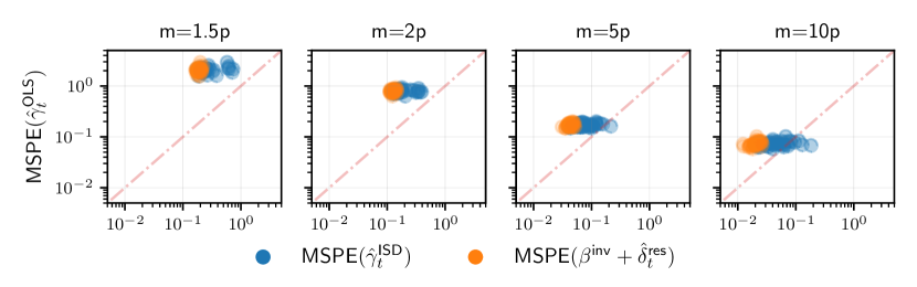
The ISD framework is particularly helpful in scenarios in which the size of the available adaptation window is small (two first plots from the left in Figure 6). A further benefit of the ISD estimator is that it allows us to estimate for small lengths of the adaptation window where and OLS is not feasible.
We run a similar experiment to show (Figure 7) the average cumulative explained variance on the adaptation data over runs, both by estimators computed only on the historical data and estimators that use the adaptation data. For visualization purposes, we now consider the time-varying coefficients (before the transformation using ) equal to , where is the coefficient index, in the historical data, and constantly equal to , and in three consecutive time windows of size on the time points after the historical data. We estimate and on a rolling adaptation window of size . The plot in Figure 7 shows that, on average, the ISD framework, by exploiting invariance properties in the observed data, allows us to accurately explain the variance of the response by using small windows for time adaptation, significantly improving on the OLS solution in the same time windows.

6 Summary
We propose Invariant Subspace Decomposition (ISD), a framework for invariance-based time adaptation. Our method relies on the orthogonal decomposition of the parameter space into an invariant subspace and a residual subspace , such that the maximizer of the explained variance over is time-invariant. The estimation of the invariant component on a large historical dataset and the reduced dimensionality of with respect to the original parameter space allow the ISD estimator to improve on the prediction accuracy of existing estimation techniques. We provide finite sample guarantees for the proposed estimation method and additionally support the validity of our theoretical results through simulated experiments.
Future developments of this work may investigate the presented problem in the case of nonlinear time-varying models, and study how to incorporate the ISD framework in specific applied settings such as contextual bandits.
Acknowledgments
NP and ML are supported by a research grant (0069071) from Novo Nordisk Fonden.
References
- Bühlmann and Meinshausen (2015) P. Bühlmann and N. Meinshausen. Magging: maximin aggregation for inhomogeneous large-scale data. Proceedings of the IEEE, 104(1):126–135, 2015.
- De Lathauwer (2008) L. De Lathauwer. Decompositions of a higher-order tensor in block terms—part ii: Definitions and uniqueness. SIAM Journal on Matrix Analysis and Applications, 30(3):1033–1066, 2008.
- Durbin and Koopman (2012) J. Durbin and S. J. Koopman. Time series analysis by state space methods, volume 38. OUP Oxford, 2012.
- Fan and Zhang (2008) J. Fan and W. Zhang. Statistical methods with varying coefficient models. Statistics and its Interface, 1(1):179, 2008.
- Févotte and Theis (2007) C. Févotte and F. J. Theis. Pivot selection strategies in jacobi joint block-diagonalization. In International Conference on Independent Component Analysis and Signal Separation, pages 177–184. Springer, 2007.
- Gutch and Theis (2012) H. W. Gutch and F. J. Theis. Uniqueness of linear factorizations into independent subspaces. Journal of Multivariate Analysis, 112:48–62, 2012.
- Hastie and Tibshirani (1993) T. Hastie and R. Tibshirani. Varying-coefficient models. Journal of the Royal Statistical Society Series B: Statistical Methodology, 55(4):757–779, 1993.
- Horn and Johnson (2012) R. A. Horn and C. R. Johnson. Matrix analysis. Cambridge university press, 2012.
- Magliacane et al. (2018) S. Magliacane, T. van Ommen, T. Claassen, S. Bongers, P. Versteeg, and J. M. Mooij. Domain adaptation by using causal inference to predict invariant conditional distributions. In S. Bengio, H. Wallach, H. Larochelle, K. Grauman, N. Cesa-Bianchi, and R. Garnett, editors, Advances in Neural Information Processing Systems 31, pages 10846–10856. Curran Associates, Inc., 2018.
- Meinshausen and Bühlmann (2015) N. Meinshausen and P. Bühlmann. Maximin effects in inhomogeneous large-scale data. The Annals of Statistics, 43(4):1801–1830, 2015.
- Mourtada (2022) J. Mourtada. Exact minimax risk for linear least squares, and the lower tail of sample covariance matrices. The Annals of Statistics, 50(4):2157–2178, 2022.
- Murota et al. (2010) K. Murota, Y. Kanno, M. Kojima, and S. Kojima. A numerical algorithm for block-diagonal decomposition of matrix-algebras with application to semidefinite programming. Japan Journal of Industrial and Applied Mathematics, 27(1):125–160, 2010.
- Nion (2011) D. Nion. A tensor framework for nonunitary joint block diagonalization. IEEE Transactions on Signal Processing, 59(10):4585–4594, 2011.
- Peters et al. (2016) J. Peters, P. Bühlmann, and N. Meinshausen. Causal inference by using invariant prediction: identification and confidence intervals. Journal of the Royal Statistical Society Series B: Statistical Methodology, 78(5):947–1012, 2016.
- Pfister et al. (2019a) N. Pfister, P. Bühlmann, and J. Peters. Invariant causal prediction for sequential data. Journal of the American Statistical Association, 114(527):1264–1276, 2019a.
- Pfister et al. (2019b) N. Pfister, S. Weichwald, P. Bühlmann, and B. Schölkopf. Robustifying independent component analysis by adjusting for group-wise stationary noise. Journal of Machine Learning Research, 20(147):1–50, 2019b.
- Pfister et al. (2021) N. Pfister, E. G. William, J. Peters, R. Aebersold, and P. Bühlmann. Stabilizing variable selection and regression. The Annals of Applied Statistics, 15(3):1220–1246, 2021.
- Rojas-Carulla et al. (2018) M. Rojas-Carulla, B. Schölkopf, R. Turner, and J. Peters. Causal transfer in machine learning. Journal of Machine Learning Research, 19(36):1–34, 2018.
- Schott (2016) J. R. Schott. Matrix analysis for statistics. John Wiley & Sons, 2016.
- Stojanov et al. (2021) P. Stojanov, Z. Li, M. Gong, R. Cai, J. Carbonell, and K. Zhang. Domain adaptation with invariant representation learning: What transformations to learn? In M. Ranzato, A. Beygelzimer, Y. Dauphin, P. Liang, and J. W. Vaughan, editors, Advances in Neural Information Processing Systems, volume 34, pages 24791–24803. Curran Associates, Inc., 2021.
- Sun et al. (2017) B. Sun, J. Feng, and K. Saenko. Correlation alignment for unsupervised domain adaptation. In Domain Adaptation in Computer Vision Applications, pages 153–171. Springer, 2017.
- Tichavsky and Koldovsky (2012) P. Tichavsky and Z. Koldovsky. Algorithms for nonorthogonal approximate joint block-diagonalization. In 2012 Proceedings of the 20th European signal processing conference (EUSIPCO), pages 2094–2098. IEEE, 2012.
- Tichavsky and Yeredor (2008) P. Tichavsky and A. Yeredor. Fast approximate joint diagonalization incorporating weight matrices. IEEE Transactions on Signal Processing, 57(3):878–891, 2008.
- Tichavskỳ et al. (2012) P. Tichavskỳ, A. Yeredor, and Z. Koldovskỳ. On computation of approximate joint block-diagonalization using ordinary ajd. In International Conference on Latent Variable Analysis and Signal Separation, pages 163–171. Springer, 2012.
- Zhao et al. (2019) H. Zhao, R. T. Des Combes, K. Zhang, and G. Gordon. On learning invariant representations for domain adaptation. In International conference on machine learning, pages 7523–7532. PMLR, 2019.
Appendix A Supporting examples and remarks
A.1 Example of non-uniqueness of an irreducible orthogonal partition
Assume that for all the covariance matrix of takes one of the following two values (and each value is taken at least once in )
Define for all the linear spaces , where is the -th vector of the canonical basis. Then since and are (block) diagonal the partition is an irreducible orthogonal partition w.r.t. . Consider now the orthonormal matrix
It holds that
Therefore, the spaces
also form an irreducible orthogonal partition w.r.t. (this follows, for example, from Proposition 1) but .
Then, if we assume for example that , given the first partition we obtain , whereas given the second partition it holds that and and therefore , leading to Assumption 1 not being satisfied.
A.2 Threshold selection for opt-invariant subspaces
In the simulations, we select the threshold in (18) by cross-validation. More in detail, we define the grid of possible thresholds by
where . We then split the historical data into disjoint blocks of observations, and for all denote by and the observations in the -th block and by and the remaining historical data. For all possible thresholds we proceed in the following way. For all folds , we compute an estimate for the invariant component as in (19) using and , which we denote by . Inside the left-out -th block of observations, we then consider a rolling window of length and the observation at immediately following the rolling window: we compute the residual parameter as in (21) using the observations in the rolling window, and evaluate the empirical explained variance by on the observation at , i.e.,
We repeat this computation for all possible , where denotes the time points in the -th block of observations excluding the first observations, and define . For all , we denote the average explained variance over the folds by and the standard error (across the folds) of such explained variance as . Moreover, let . Then, we choose the optimal threshold as
which is the most conservative (lowest) threshold such that the corresponding explained variance is within (in our simulations, we choose ) standard errors (computed across the folds) of the maximal explained variance.
A.3 Methods and computational complexity of joint block diagonalization
In the context of joint block diagonalization, we can differentiate between methods that solve the exact problem (JBD), i.e., are such that the transformed matrices have exactly zero off-block diagonal entries, and approximate methods (AJBD), which assume the presence of noise and aim to minimize the off-block diagonal entries, without necessarily setting them to zero.
JBD is in general an easier problem, and algorithms that solve it have been shown to achieve polynomial complexity (see, e.g., Murota et al., 2010; Tichavskỳ et al., 2012). Many of these methods, e.g., the one presented by Murota et al. (2010), are based on eigenvalue decompositions. Alternatively, as shown by Tichavskỳ et al. (2012), some algorithms that solve the problem of approximate joint diagonalization (AJD) of a set of matrices, such as uwedge developed by Tichavsky and Yeredor (2008), can also be used for JBD. More in detail, a solution to AJD is a matrix that maximally jointly diagonalizes a set of matrices by minimizing the average value of the off-diagonal entries; if the matrices in the set cannot be exactly jointly diagonalized, the transformed matrices will have some non-zero off-diagonal elements. Adding an appropriate permutation of the columns of the joint diagonalizer allows to reorganize the non-zero off-diagonal elements into blocks, leading to jointly block diagonal matrices: in Section of their work Gutch and Theis (2012) argue that if the matrices to be block diagonalized are symmetric, then the solution found in this way is also an optimal JBD solution.
However, in general, methods for JBD cannot be directly applied to solve AJBD. Algorithms that solve AJBD directly – based on the iterative optimization of a cost function via matrix rotations – have been developed, for example, by Tichavsky and Koldovsky (2012) and Févotte and Theis (2007), but require the number of diagonal blocks to be known in advance. Alternatively and similarly to how JBD can be solved by AJD methods, one can also, with some slight modifications, use AJD methods to solve AJBD. More specifically, some heuristics need to be used to determine the size of the blocks: these can consist, for example, in setting a threshold for the non-zero off-block-diagonal elements in the transformed matrices.
In the (orthogonal) settings considered here, we have found the last approach to work effectively. More specifically, in Section 4.1.1, we have denoted by the AJD solution for the set of estimated covariance matrices . Similarly to how Tichavsky and Koldovsky (2012) suggest to determine a permutation of the AJD result, we proceed in the following way. To discriminate the non-zero off-block-diagonal entries in these matrices, we start by computing the following auxiliary matrix using
where the maximum is taken element-wise. The matrix captures in its off-diagonal entries the residual correlation among the components identified by AJD, for all the jointly diagonalized matrices. For all thresholds , we let denote one of the permutation matrices satisfying that is a block diagonal matrix if all entries smaller than are considered zero. We then define the optimal threshold by
where denotes the average value of off-block-diagonal entries (determined by the threshold ) of a matrix, is the total number of entries in the blocks induced by and is a regularization parameter. The penalization term is introduced to avoid always selecting a zero threshold, and the regularization parameter is set to where denotes the minimum eigenvalue. The optimal permutation is then and the estimated irreducible joint block diagonalizer is .
A.4 Further simulation details: MSPE comparison
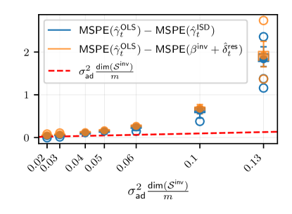
In Section 5.2 we present a simulated experiment in which we compare the ISD estimator and the OLS estimator on the time adaptation task. Figure 6 shows that the difference in the MSPE for and is positive and decreases for increasing values of . To further support the statement of Theorem 3, we show in Figure 8 the value of such difference against , when computing both with the estimated and oracle invariant component. The figure shows that the difference in the MSPEs indeed satisfies the bound stated in Theorem 3, i.e., it is always greater than . Moreover, it shows that for small values of the gain in using the ISD estimator over the OLS is even higher than what the theoretical bound suggests, indicating that it is not sharp for small .
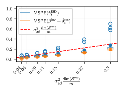
We further show in Figure 9 the MSPE of (again computed both with the estimated and oracle invariant component) against , obtaining in this case an empirical confirmation of the first bound presented in Theorem 3.
Appendix B Extension to non-orthogonal subspaces
In Section 2.1 we have defined an orthogonal partition w.r.t. as a collection of pairwise orthogonal linear subspaces of satisfying (6). Finding the orthogonal subspaces that form the partition means in particular finding a rotation of the original -space such that each subspace is spanned by a subset of the rotated axes, and the coordinates of the projected predictors onto one subspace are uncorrelated with the ones in the remaining subspaces. In this section, we show that orthogonality of the subspaces in the partition is not strictly required to obtain a separation of the true time-varying parameter of the form (7), that is, more general invertible linear transformations can be considered besides rotations. In particular, we briefly present results similar to the ones obtained throughout Section 2 but where the subspaces in the partition are not necessarily orthogonal. To do so, we define a collection of (not necessarily orthogonal) linear subspaces with and satisfying (6) a partition w.r.t. (of cardinality ), and further call it irreducible if it is of maximal cardinality. A partition w.r.t. can still be identified through a joint block diagonalization of the covariance matrices as described in Section 2.1.1 but with an adjustment. More specifically, instead of assuming that the joint diagonalizer is an orthogonal matrix, we only assume it is invertible and for all , the columns of are orthonormal vectors. A version of Proposition 1 in which the resulting partition is not necessarily orthogonal follows with the same proof. Moreover, similarly to the orthogonal case, the uniqueness of an irreducible partition w.r.t. is implied by the uniqueness of an irreducible non-orthogonal joint block diagonalizer for ; explicit conditions under which such uniqueness holds can be found for example in the work by Nion (2011). In the results presented in the remainder of this section we adopt the same notation introduced in Section 2.1.1, and we additionally define the matrix .
A partition w.r.t. of cardinality allows us to decompose the true time-varying parameter into the sum of components. To obtain such a decomposition via non-orthogonal subspaces, oblique projections need to be considered in place of orthogonal ones. Oblique projections are defined (see, e.g., Schott, 2016) for two subspaces such that and a vector as the vectors and such that : is called the projection of onto along , and the projection of onto along . For a partition w.r.t. , we denote by the oblique projection matrix onto along : this can be expressed in terms of a (non-orthogonal) joint block diagonalizer corresponding to the partition as . Orthogonal partitions w.r.t. are a special case of partitions w.r.t. . In particular, if the subspaces are pairwise orthogonal, it holds for all that .
By definition of oblique projections, for all , we can express as
Similarly to how we define opt-invariance on for orthogonal subspaces in Section 2.1, we say that a subspace in a partition w.r.t. is proj-invariant on if it satisfies for all that
By Lemma 4 it follows that for orthogonal partitions proj-invariance is equivalent to opt-invariance. For an irreducible partition w.r.t. , we now define the invariant subspace and residual subspace as
It follows directly by the definition of partitions that is a partition w.r.t. . Moreover, is proj-invariant on since . We finally define the invariant and residual components by
We show in the following proposition that the expressions (13) and (15) used to construct our estimators for the invariant and residual component in the case of orthogonal partitions, remain valid in the case of non-orthogonal partitions.
Proposition 3.
Let be a partition w.r.t. and let be a joint block diagonalizer corresponding to that partition. Then, the following results hold.
-
(i)
For all and for all
(24) -
(ii)
is time-invariant over and
-
(iii)
Proposition 3 implies in particular that, apart from the joint block diagonalization differences, estimating and in the non-orthogonal case can be done as described in Section 4. Moreover, it holds that the parameter defined for non-orthogonal partitions w.r.t. is still a time-invariant parameter. Under a generalization assumption analogous to Assumption 2, has positive explained variance at all time points and can be used to at least partially predict (we have not added this result explicitly). In addition, also in the non-orthogonal case the estimation of the residual component only requires to estimate a reduced number of parameters, that is, .
In the case of non-orthogonal partitions, however, we cannot directly interpret ISD as separating the true time-varying parameter into two separate optimizations of the explained variance over and .
Example 6 (non-orthogonal irreducible partition).
Let with covariance matrix that for all takes one of the following values
These matrices are in block diagonal form and in particular the submatrices forming the first diagonal block do not commute. This implies that an irreducible (orthogonal) joint block diagonalizer for these matrices is the three-dimensional identity matrix , and the diagonal blocks cannot be further reduced into smaller blocks using an orthogonal transformation. It also implies that an irreducible orthogonal partition w.r.t. is given by with and , where is the -th vector of the canonical basis for .
There exists, however, a non-orthogonal joint diagonalizer for these matrices, i.e., a non-orthogonal matrix such that is diagonal. It is given by
induces an irreducible partition w.r.t. by
Let and be the invariant subspaces associated with the irreducible orthogonal partition and the irreducible partition , respectively. As any irreducible orthogonal partition w.r.t. is also a partition w.r.t. , it in general holds that
Moreover, as in the explicit example above, the inequality can be strict.
Appendix C Auxiliary results
Lemma 1.
Let be a symmetric invertible matrix, an orthogonal block diagonalizer of and disjoint subsets satisfying
Then it holds for all that
where .
Proof.
The pseudo-inverse of a matrix is defined as the unique matrix satisfying: (i) , (ii) , (iii) and (iv) .
Fix and define and . Moreover, define and for all , . We now verify that conditions (i)-(iv) hold for and and hence is indeed the pseudo-inverse. Conditions (ii) and (iv) hold by symmetry of and . For (i) and (iii), first observe that by the properties of orthogonal matrices it holds that , and, due to the block diagonal structure of ,
| (25) |
Hence we get that . For (i), we now get
Similarly, for (iii) we get
This completes the proof of Lemma 1.
∎
Lemma 2.
Let and let be an orthogonal partition w.r.t. .333 This is defined analogously to an orthogonal partition w.r.t. . Then, there exists a joint block diagonalizer of . More precisely, there exists an orthonormal matrix such that for all the matrix is block diagonal with diagonal blocks , and of dimension , where indexes a subset of the columns of . Moreover, .
Proof.
Let be an orthonormal matrix with columns such that for all there exists such that . Such a matrix can be constructed by selecting an orthonormal basis for each of the disjoint subspaces . Furthermore, assume that the columns of are ordered in such a way that for all with it holds for all and that . As the matrix is orthogonal, it holds for all that the projection matrix can be expressed as and hence using the definition of orthogonal partition (see 6) it holds that, for all ,
where for all we defined . ∎
Lemma 3.
Let be an orthogonal partition w.r.t. . Then it holds for all that
and, for all ,
| (26) |
Proof.
Let be an orthonormal matrix such that, for all , is block diagonal with diagonal blocks of dimensions . Such a matrix exists by Lemma 2 and each diagonal block is given by and the projection matrix can be expressed as . Now, for an arbitrary it holds using the linear model (1) that and hence we use to get the following expansion
By the properties of orthogonal matrices it holds that , and, due to the block diagonal structure of ,
| (27) |
This implies that and therefore
In the last equality we have used that , by Lemma 1. This completes the proof of Lemma 3. ∎
Lemma 4.
Let and let be an orthogonal partition w.r.t. . Then it holds for all and for all that
| (28) |
Moreover, if, in addition, , it holds for all that
where .
Proof.
For all , for all and for all it holds that
| (29) |
where the first equality follows by (2) and the third equality follows from the definition of an orthogonal partition. It follows that
where denotes the gradient. The equation has a unique solution in given by . To see this, observe that all other solutions in are given, for an arbitrary vector , by
| (30) |
where denotes the identity matrix. Let and be defined for the orthogonal partition w.r.t. as in Lemma 2. We now observe that
| (31) | ||||
where the first equality follows from Lemma 1, since jointly block diagonalizes the matrices by Lemma 2. We can therefore rewrite (30) as
For all , this expression equals . For all , it is not in . It now suffices to show that , which follows from the following computation
where the first and third equality follow from Lemma 3.
We now observe that for all and for all it follows from (29) that
which has gradient
The equation has solution equal to
By Lemma 1, it holds that and therefore . In order to apply Lemma 1, we in particular use that is such that, for all , is block diagonal with diagonal blocks given, for all , by . This implies that is also block diagonal with diagonal blocks . Moreover, its inverse is block diagonal and, by the properties of orthogonal matrices, its diagonal blocks are . It now remains to show that this is also the only solution in . All other solutions in are given, for an arbitrary vector , by
The equality follows from the following computation
where is the matrix introduced in (31). The first equality follows again from Lemma 1. For all , equals . For all , is not in . This concludes the proof for Lemma 4. ∎
Lemma 5.
is opt-invariant on .
Proof.
That is opt-invariant on can be seen from the following computations. It holds for all that
The first equality holds by Lemma 4, since is indeed an orthogonal subspace partition w.r.t. , see Lemma 6. The second equality follows from the definition of and can be proved by Lemma 3 and, observing that the set of subspaces is an orthogonal partition w.r.t. . The third equality holds by Lemma 4 and the fourth by definition of an opt-invariant subspace on . ∎
Lemma 6.
is an orthogonal partition w.r.t. .
Proof.
Let be a fixed irreducible orthogonal partition w.r.t. according to which and are defined. By orthogonality of the subspaces in the partition and by definition of and , . Moreover, by definition of orthogonal partition w.r.t. , it holds that
∎
Lemma 7.
Let be a set of symmetric strictly positive definite matrices. If there exists a matrix that has all distinct eigenvalues, then any two irreducible joint block diagonalizers for the set are equal up to block permutations and block-wise isometric transformations.
Proof.
We start by observing that if a matrix is symmetric and has all distinct eigenvalues, then its eigenvectors are orthogonal to each other and unique up to scaling. We define as the orthonormal matrix whose columns are eigenvectors for : is then uniquely defined up to permutations of its columns.
We now exploit the results by Murota et al. (2010) used in the construction of an irreducible orthogonal joint block diagonalizer for a set of symmetric matrices (not necessarily containing a matrix with all distinct eigenvalues). In the following, we translate all the useful results by Murota et al. (2010) in our notation introduced for joint block diagonalizers in Section 2.1.1. Murota et al. (2010) show in Theorem that there exists an irreducible orthogonal joint block diagonalizer such that, for all , , where , are such that , and are square matrices (common diagonal blocks). Here denotes the direct sum operator for matrices and the Kronecker product. They further propose to partition the columns of the matrix into subsets, each denoted by , with indexing the diagonal blocks and denoting the subset of indexes corresponding to the selected columns in , such that, for all , . They then argue that, as a consequence of Theorem , the spaces spanned by such subsets of columns, i.e.,
are uniquely defined. We therefore only need to prove that, if at least one matrix in the set has all distinct eigenvalues, then for all , . Such condition implies that the diagonal blocks indexed by , , are irreducible, and .
The uniqueness of the spaces then implies the uniqueness of the irreducible joint block diagonalizer up to block permutations and block-wise isometric transformations. To show this result, we now use Murota et al. (2010, Proposition 1). In particular, if the set contains at least one matrix with all distinct eigenvalues then the assumptions of Proposition are satisfied. Let be the set of eigenspaces of and for all let . The proposition then implies that for all there exists such that . Moreover, for all such that it holds that . As a consequence, we obtain that, since the eigenvalues of are distinct, and therefore for all , . This concludes the proof for Lemma 7.
∎
Lemma 8.
Let be an irreducible orthogonal partition w.r.t. . Then, for all such that is opt-invariant on , it holds for all that
Moreover, is time-invariant on .
Proof.
For all opt-invariant on and for all it holds that
where we used the definition of opt-invariance on for the second equality and Lemma 4 for the third and fourth equality. Since the result holds for all , it also follows that
We now need to prove for all that . To see this, fix . Then
The last equality follows from the definition of an orthogonal partition w.r.t. . ∎
Lemma 9.
Let be an irreducible orthogonal partition w.r.t. and let be the corresponding invariant subspace. Moreover, let and . Finally, let be the submatrix of an arbitrary irreducible joint block diagonalizer corresponding to the irreducible orthogonal partition w.r.t. whose columns span . Then,
Proof.
Expanding the definition of , we obtain that
The fourth equality follows from Lemma 4. The fifth equality follows by Lemma 1 (see the proof of Lemma 4). In the last equality we used that , which follows from the properties of orthogonal matrices and the block diagonal structure of : these imply that and
∎
Appendix D Proofs
D.1 Proof of Theorem 1
Proof.
Let be an irreducible orthogonal partition w.r.t. and define and as in (10). By Assumption 2, form an orthogonal partition w.r.t. and is opt-invariant on . Therefore, using Lemma 4, we get for all that
Furthermore, opt-invariant on implies that the first term, , does not depend on and hence it holds for all that
D.2 Proof of Proposition 1
Proof.
For all , let denote the submatrix of formed by the columns indexed by . Then, the orthogonal projection matrix onto the subspace can be expressed as . It follows for all that
where the last equality holds since is the -th (off-diagonal) block of , which is zero due to the block diagonal structure of . Irreducibility of the orthogonal partition follows from the irreducibility of the joint block diagonal decomposition. ∎
D.3 Proof of Proposition 2
Proof.
(i) First, observe that, by Lemma 6, is an orthogonal partition w.r.t. and that, by Lemma 5, is opt-invariant on . Then, by definition of and by Lemma 8 we get for all that
(ii) We need to prove for all that . To see this, fix . Then
where the third equality uses by Proposition 2 and the last equality follows from the fact that , are an orthogonal partition w.r.t. by Lemma 6.
(iii) Let denote the set of all time-invariant parameters over . By assumption, we have that . Moreover, by point , we have that . Therefore, by definition of we obtain that . This completes the proof of Proposition 2. ∎
D.4 Proof of Theorem 2
Proof.
Under Assumptions 1 and 2 and using the definitions of and , we can write the explained variance of at time for the true time varying parameter as
Using this expansion, we get, since , for all that
Therefore,
Since by assumption it holds that is opt-invariant on , it further holds that for all
The claim follows from the definition of . ∎
D.5 Proof of Theorem 3
Proof.
We assume without loss of generality that the observed predictors have zero mean in . Alternatively, as mentioned in Section 4.1.2, a constant term could be added to to account for the mean. We also observe that and are both unbiased estimators for and , respectively (this can be checked using standard OLS analysis). We now start by computing the out-of-sample MSPE for .
where we have used that . We further observe that
where is a diagonal matrix whose diagonal elements are the error variances at each observed time steps, . Let and . Then,
where denotes the Loewner order, and it follows from , with denoting an -dimensional diagonal matrix with diagonal elements all equal. We have used in particular that for two symmetric matrices such that and a matrix it holds that (see, for example, Theorem 7.7.2. by Horn and Johnson, 2012). Using this relation and Jensen’s inequality, we obtain that the first term in is lower bounded by
where . Using now that, by assumption, is an orthogonal partition w.r.t. , let be defined for such a partition as in Lemma 2 and let be the submatrix of whose columns form an orthonormal basis for , such that . Moreover, let and denote, as in Lemma 2, the diagonal block corresponding to of the block diagonal matrices and , respectively. By the properties of orthogonal matrices, . For all , let denote the -th eigenvalue in decreasing order. Then, we can further express the above lower bound as
where we define . The same term in is upper bounded by
where . Proceeding in a similar way, we can express the second term in as
where . Since we have assumed that for all the distribution of does not change, by Jensen’s inequality and by the fact that (see Lemma 6 and (31)) we have that , and . Moreover, we can find an upper bound for in the following way.
Summarizing, we obtain that
and
where is the constant introduced in the theorem statement.
We now compute the MSPE of .
We can further express as
In particular, the second term in the above sum also appears in . Taking now the difference between the MSPE of and , we obtain that
We have already obtained an upper bound for the second term in the difference, namely . For the first term, we can make the same considerations made above for and . In particular,
where
satisfies and (as for , we observe that ). Therefore, we obtain that
and
where . In particular, this difference is always positive if is sufficiently large. Finally, we can observe that the expected explained variance (23) for , where or , is
and therefore the same inequalities found for the MSPEs difference equivalently hold for . ∎
D.6 Proof of Proposition 3
Proof.
(i) By definition of a (non-orthogonal) joint block diagonalizer, it holds for all that the matrix is block diagonal with diagonal blocks , . Define now the matrix , and observe that the following relations hold
The last relation is obtained by observing that
Moreover, . We observe that, because , it holds for all that , that is, the space spanned by the columns of is orthogonal to the space spanned by the columns of . Moreover, the matrix is an oblique projection matrix onto along . Fix . Then, using these relations we obtain that
The fourth equality follows from the block diagonal structure of , which implies that, for all , .
(ii) By definition of and using point (i) of this proposition and that form a partition w.r.t. , we obtain that, for all ,
We now observe that is the OLS solution of regressing onto (as we assume all variables have zero mean). Moreover, this quantity is constant by proj-invariance of . In particular, this means that , which implies that
Therefore, .
(iii) The claim follows from the definition of , from the fact that forms a partition w.r.t. and from point (i) of this proposition. ∎