NNLO QCD corrections to polarized semi-inclusive DIS
Abstract
Polarized semi-inclusive deep-inelastic scattering (SIDIS) is a key process in the quest for a resolution of the proton spin puzzle. We present the complete results for the polarized SIDIS process at next-to-next-to-leading order (NNLO) in perturbative quantum chromodynamics. Our analytical results include all partonic channels for the scattering of polarized leptons off hadrons and a spin-averaged hadron identified in the final state. A numerical analysis of the NNLO corrections illustrates their significance and the reduced residual scale dependence in the kinematic range probed by the future Electron-Ion-Collider EIC.
Deep-inelastic scattering (DIS) of leptons off hadrons provides valuable information on the structure of hadrons at high energies in terms of their partonic constituents namely quarks, anti-quarks and gluons, and also of the underlying strong interaction dynamics through quantum chromodynamics (QCD) Blümlein (2013). The DIS structure functions (SFs), encoding this information, are subject to QCD factorisation that separates short-distance dynamics accessible in perturbation theory from the long-distance (non-perturbative) one. The perturbative part, so-called coefficient functions (CFs), is computed in powers of the strong coupling , while the non-perturbative parton dynamics inside the hadron are parameterised in terms of parton distribution functions (PDFs), generally extracted from cross section data Workman and Others (2022). Semi-inclusive DIS (SIDIS) with an identified hadron in the final state adds to the factorisation formalism parton fragmentation functions (FFs) Metz and Vossen (2016), which encode the parton dynamics in their recombination to form hadrons.
Polarized DIS is a key process for the resolution of the long-standing proton spin puzzle. It gives access to the longitudinal spin structure of hadrons Aidala et al. (2013), parameterised by helicity (spin-dependent) PDFs de Florian et al. (2009, 2014); Nocera et al. (2014). The proton spin can be determined from a sum-rule for those helicity PDFs. Polarized SIDIS is particularly important for the separate extraction of (anti-)quark helicity PDFs from data. This makes it a prominent observable to be measured at the upcoming Electron-Ion collider (EIC) at the Brookhaven National Laboratory Abdul Khalek et al. (2022). The unique opportunities to study it at the EIC challenge the accuracy of available QCD theory predictions and provide motivation for their improvements, which will be addressed in this letter.
The reaction defines the SIDIS process, where , (, ) are momenta of incoming and outgoing leptons (hadrons), respectively, and the virtual photon momentum squared, , is large. The QCD improved parton model allows to express infrared safe observables in SIDIS through CFs, PDFs and FFs. The hadron level cross section for unpolarized (spin averaged) SIDIS is given in terms of SFs . Exact results for the CFs of up to next-to-leading order (NLO) in perturbative QCD were obtained long ago Altarelli et al. (1979); Furmanski and Petronzio (1982) and the resummation of large threshold logarithms for SIDIS has been accomplished up to third order in QCD Cacciari and Catani (2001); Anderle et al. (2013a, b); Abele et al. (2021, 2022). Recently, thanks to state-of-the-art theoretical developments in the computation of Feynman loop and phase-space integrals, the CFs have been computed to next-to-next-to-leading order (NNLO) accuracy. We have presented the first NNLO results (non-singlet parton channels and leading color approximation) in Goyal et al. (2023). Subsequently, the complete results for the CFs of (all parton channels and full color dependence) have become available Bonino et al. (2024a); Goyal et al. (to appear) and both results agree with each other for all the channels.
Thus far, the description of polarized SIDIS in QCD has only been available at NLO accuracy de Florian et al. (1998). In this letter we present, for the first time, the full NNLO QCD corrections. Polarized SIDIS is defined by the asymmetry
where denote the (anti-)parallel spin-orientations of the colliding electron and hadron. Here is the Bjorken variable, the inelasticity, and the scaling variable of the identified hadron. The hadronic cross section above factorises into spin-dependent leptonic and hadronic tensors and ,
| (1) |
Here , with the spin vector of the incoming lepton, and can be expressed in terms of spin-dependent SFs and as
| (2) |
with Lorentz tensors = and = , and being the spin vector of the incoming hadron. For longitudinal polarization of the incoming hadron, is the dominant SF in the hadronic cross section,
| (3) |
where is the fine structure constant. With QCD factorisation at scale the SF takes the form
| (4) |
where = are the spin-dependent PDFs and denote the spin-averaged FFs. Here the momentum fraction is carried by the initial parton ‘’ of incident hadron and by the hadron with respect to the final state parton ‘’. The CFs are computable in perturbative QCD in powers of the strong coupling, , at the renormalization scale ,
| (5) |
where we have suppressed the scaling variables. is related to the parton level scattering cross sections through projection with ,
| (6) |
where the projector in space-time dimensions reads,
| (7) |
is the spin-dependent amplitude for the process , where the parton ‘’ fragments into hadron . Here denotes the spin of the incoming parton . is the phase space for the final state particles consisting of and . denotes the summation over final state spin/polarization and their color quantum numbers in addition to the average over colors of incoming parton .
At leading order (LO) in perturbation theory, the partonic cross sections in eq. (6) receive a contribution from . At NLO, we consider one-loop corrections to the Born process , the real emission and the gluon-initiated sub-processes. At NNLO, we include two-loop corrections to the Born process , one-loop contributions to the single-gluon real emission , and double real emissions , and , where can be of same or of different flavour as . Note that in every sub-process, we need to include fragmentation contributions from each final state parton.
Beyond LO in perturbative QCD, we encounter both ultraviolet (UV) and infrared (IR) singularities. The latter are due to the presence of soft and collinear partons. We regulate these singularities using dimensional regularisation with space-time dimensions. The projection of spin-dependent partonic amplitudes squared in eq. (6) requires Dirac matrices or the Levi-Civita tensor for polarized quarks or gluons, respectively, see, e.g. Zijlstra and van Neerven (1994). Since and the Levi-Civita tensor are intrinsically four-dimensional objects, their treatment in dimensions requires some prescription. Although, several schemes to define them in dimensions have been proposed, none of them is known to preserve chiral Ward identity. A given prescription then requires an additional renormalisation constant or an evanescent counter-term to preserve this identity. In this letter, we use Larin’s prescription Larin (1993) and replace by . The product of two Levi-Civita tensors is computed through the determinant of Kronecker deltas defined in dimensions. The UV singularities are regulated through the renormalisation of the strong coupling at the scale . The IR singularities cancel among virtual and real emission processes, except those from either incoming parton or tagged final state partons that are collinear to rest of partons. Mass factorisation guarantees that the partonic cross sections in eq. (6) factorise into the spin-dependent Altarelli-Parisi (AP) kernels of PDFs and of FFs, appropriately convoluted with the finite CF () at an arbitrary scale (suppressed here for brevity),
| (8) |
where , summation over is implied and () denotes a convolution over the scaling variable corresponding to PDFs (FFs), cf. eq. (NNLO QCD corrections to polarized semi-inclusive DIS).
The polarized space-like AP kernels () are known at the order required Mertig and van Neerven (1996); Vogelsang (1996a, b); Moch et al. (2014); Blümlein et al. (2021); Blümlein et al. (2022a, b). Since the partonic cross sections in eq.(8) are derived in Larin’s scheme, these spin-dependent AP kernels need to be taken in the same scheme, see Moch et al. (2014). On the other hand, the spin-averaged time-like AP kernels () are taken in the standard scheme Almasy et al. (2012); Chen et al. (2021).
The hadronic cross section (and the SF ) is independent of the prescription for . Thus, QCD factorisation allows to write in eq. (NNLO QCD corrections to polarized semi-inclusive DIS) as
| (9) |
where the subscript in and denotes PDFs and CFs defined using Larin’s scheme. It is straightforward to convert these quantities into ones Moch et al. (2014). The CFs in the scheme are obtained by transforming to PDFs through and CFs to CFs, . The finite renormalization constants are dependent on and well known Matiounine et al. (1998); Ravindran et al. (2004); Moch et al. (2014). We present the CFs in the scheme in an ancillary file. The flavor-nonsinglet CFs of polarized SIDIS agree with those of the SF , cf. Goyal et al. (to appear). The latter require a renormalization of the axial current and a kinematics independent finite renormalization from the Larin to the scheme Larin and Vermaseren (1993); Ahmed et al. (2015). We find full agreement, which checks the scheme transformations applied. Before we proceed to report the numerical impact of NNLO contributions to , we briefly describe, how the cross sections in eq. (6) are computed in Larin’s scheme (denoted by ).
Beyond LO, the contributions to can be classified into three categories: pure virtual (VV), pure real emissions (RR) and interference of real emission and virtual (RV). The VV part gets contributions from one-loop and two-loop virtual corrections to the Born process. The latter can be obtained using the quark form factor, see Lee et al. (2022). For the rest, we follow the standard Feynman diagrammatic approach. We use QGRAF Nogueira (1993) to generate Feynman diagrams and use a set of in-house routines written in FORM Kuipers et al. (2013); Ruijl et al. (2017), to convert the output of QGRAF into a suitable format to apply Feynman rules and to perform Dirac algebra, Lorentz contractions and simplifications of color factors. The computations of phase-space integrals are challenging compared to those required for inclusive cross sections because of the presence of an additional constraint . The two-body phase-space over one-loop Feynman integrals that appear in RV and three-body phase space integrals in RR are simplified with reverse unitarity Anastasiou et al. (2004, 2012). This method allows us to apply loop-integration techniques, namely integration-by-parts identities (IBP) Chetyrkin and Tkachov (1981); Laporta (2000), to reduce the phase-space integrals to a smaller number of the master integrals (MIs). The constraint is introduced through the delta function , where =, which is replaced by a propagator-like term with or for two- and three-body final states respectively. To perform the IBP reduction, we use the Mathematica package LiteRed Lee (2014).
After IBP reduction, we end up with 7 MIs for RV and 21 MIs for RR sub-processes. Due to the delta function constraint, the results of the MIs depend on two scaling variables (). We have used two different approaches to compute these integrals. In the first approach, we choose a convenient Lorentz frame to parameterize the momenta so that the the constraint on takes the simple form and three-body phase-space integrals become three-dimensional parametric integrals, see Matsuura et al. (1989); Zijlstra and van Neerven (1992); Rijken and van Neerven (1997); Ravindran et al. (2003) for more details. We encounter two angular integrals and one parametric integral. Angular integrals reduce to Hypergeometric functions and the parametric integrals over these functions lead to multiple polylogarithms (MPLs) and Nielsen polylogarithms of weight up to three. In the second approach, we use the method of differential equations (DEs) Kotikov (1991); Argeri and Mastrolia (2007); Remiddi (1997); Henn (2013); Ablinger et al. (2016) to solve the integrals. We set up the system of differential equations of the MIs with respect to the variables using LiteRed. Each set of DEs is controlled by 2121 matrix. By an appropriate set of transformations on the set of MIs, we can express these matrices in an upper or lower-triangular form leading to the bottom-up approach of solving the DEs one by one. Alternatively, we use the elegant approach of an -factorized form Henn (2013) to reduce the DEs to canonical form with the help of the Mathematica package Libra Lee (2021). We use suitable boundary conditions to express the solution in terms of either classical polylogarithms or generalized harmonic polylogarithms (GPLs). The boundary conditions for the MIs are computed in the threshold limit from parametric integrals. We encounter four types of square-roots in the DE systems: , , , . By a set of suitable transformations on , we can express all the polylogarithms or GPLs with simple indices suitable for numerical evaluations.
The task to perform the mass factorisation for the partonic cross sections in eq. (8) to obtain finite CFs proceeds as follows. The AP kernels and in eq. (8) are pure counter-terms, containing only poles in in order to cancel the collinear singularities present in . They contain standard ‘plus’-distributions (see, e.g. Goyal et al. (2023)) and delta functions , where , in addition to regular terms. The cancellation of the collinear singularities in against those from AP kernels requires to express the former ones in terms of the same distributions and regular functions. This is the most challenging task. In the partonic cross sections we encounter terms proportional to and/or , which diverge in the respective threshold regions and/or respectively. These terms can originate either from MIs or their coefficients at the level of squared matrix elements. These singularities are regulated by and respectively resulting from phase space and loop integrals. In addition we encounter spurious singularities when or , which cancel among themselves at the end. In general, the resulting expressions contain multi-valued functions and we need to define them in different regions appropriately. We encounter different regions depending on whether with and/or or with and/or . Using Feynman’s prescription, we can analytically continue these functions smoothly from one region to other.
E.g., in the RV sub-processes, we encounter a hypergeometric function which after Pfaff transformation gives
| (10) |
Using Feynman’s prescription for scaling variables, i.e. and and the identities involving theta functions, eq. (NNLO QCD corrections to polarized semi-inclusive DIS) reduces to
where, , , , , =, and . can be analytically continued to the appropriate region and expanded in power series in , see Duplancic and Nizic (2001),Gehrmann and Remiddi (2002). Finally, collinear singularities in are exposed through
| (11) |
The resulting partonic cross sections contain double and single poles in at NLO. The former ones cancels between VV and RR terms and the latter against AP kernels in the mass factorisation eq. (8). At NNLO the leading and poles cancel among the VV, RV and RR contributions. The remaining double and single poles in cancel against the AP kernels using eq. (8). The final scheme CFs thus obtained (after transformation from the Larin scheme) can be written as,
| (12) | |||||
The soft plus virtual (SV) terms contain the double distributions , , , . Terms with single distributions, namely , , , are called partial-SV (pSV) terms and regular terms are denoted by . are in complete agreement with those of un-polarized SFs Abele et al. (2021); Goyal et al. (2023); Bonino et al. (2024a); Goyal et al. (to appear) see also Ravindran et al. (2007); Ahmed et al. (2014) and if we expand and around , then they are in complete agreement with the corresponding terms in the un-polarized case up to order and respectively, Bonino et al. (2024a); Goyal et al. (to appear); A H et al. (2021).
Our NLO results are in complete agreement with de Florian et al. (1998). At NNLO the SV terms for polarized SIDIS are identical to the unpolarized case Abele et al. (2021). The remaining contributions in eq. (12), i.e., single distributions , and regular terms are new. These results are too lengthy to be presented here and, instead included in an ancillary file.
In the following, we illustrate the numerical impact of our results for for the EIC assuming a centre of mass energy = 140 GeV. The convolution of the CFs with PDFs and FFs provides , such that at LO ( being the electric charge of quark ).
| (13) |
| (14) |
with are related to defined in eq. (5) see comments in ancillary files and denotes their convolution with in both variables and .
| (15) |
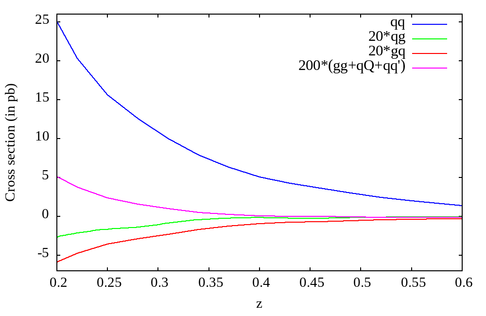
In the following, we study the numerical impact of our results. We apply NNPDFpol PDFs Ball et al. (2015), which are known at NLO level, for all three perturbative orders. For the FFs, we use NNFFPip Bertone et al. (2017), which are available up to NNLO level and we apply them at the respective perturbative order. In Fig. 1, we show the individual partonic channels contributing to the complete NNLO result at GeV and , using labels where indicates the initial parton and the fragmenting one in each partonic channel. The cross section is presented as a function of , integrating between to and between to .
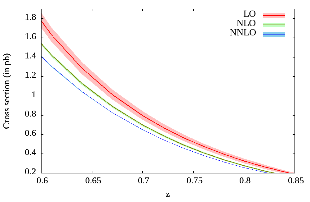
In Fig. 2, we display the total hadronic cross-section at the different perturbative orders for the same numerical inputs as above. We use active flavours and =1/128 for the electromagnetic coupling, while is taken from the PDF set NNFFPip at the respective perturbative order. The reduction of the scale dependence through the inclusion of the higher-order QCD corrections is shown by variations in the range , keeping . The central scale is the average which corresponds roughly to GeV. For illustration purposes, we restrict the -axis in Fig. 2 to the range . We observe a clear reduction of the renormalization scale uncertainties from at NLO to at NNLO when is varied by a factor of 2 around average value of . Overall, we also find good perturbative convergence with the new NNLO contributions, which are numerically significant, though. For example at , the -factor decreases from at NLO to at NNLO level.
In this letter, we report the CFs for the polarized SIDIS process at NNLO in QCD. These results close a gap in the available literature and will facilitate high precision theory predictions and will contribute to the studies of polarized PDFs and of the proton spin structure at the future EIC. A Mathematica notebook with all results for the CFs is available from the preprint server https://arXiv.org.
Acknowledgements.
Acknowledgements: We thank W. Vogelsang and S. Weinzierl for discussions. This work has been supported through a joint Indo-German research grant by the Department of Science and Technology (DST/INT/DFG/P-03/2021/dtd.12.11.21). S.M. acknowledges the ERC Advanced Grant 101095857 Conformal-EIC.Note added:
While finalizing this work, ref. Bonino et al. (2024b) has appeared on polarized SIDIS at NNLO.
References
- Blümlein (2013) J. Blümlein, Prog. Part. Nucl. Phys. 69, 28 (2013), eprint 1208.6087.
- Workman and Others (2022) R. L. Workman and Others (Particle Data Group), PTEP 2022, 083C01 (2022).
- Metz and Vossen (2016) A. Metz and A. Vossen, Prog. Part. Nucl. Phys. 91, 136 (2016), eprint 1607.02521.
- Aidala et al. (2013) C. A. Aidala, S. D. Bass, D. Hasch, and G. K. Mallot, Rev. Mod. Phys. 85, 655 (2013), eprint 1209.2803.
- de Florian et al. (2009) D. de Florian, R. Sassot, M. Stratmann, and W. Vogelsang, Phys. Rev. D 80, 034030 (2009), eprint 0904.3821.
- de Florian et al. (2014) D. de Florian, R. Sassot, M. Stratmann, and W. Vogelsang, Phys. Rev. Lett. 113, 012001 (2014), eprint 1404.4293.
- Nocera et al. (2014) E. R. Nocera, R. D. Ball, S. Forte, G. Ridolfi, and J. Rojo (NNPDF), Nucl. Phys. B 887, 276 (2014), eprint 1406.5539.
- Abdul Khalek et al. (2022) R. Abdul Khalek et al., Nucl. Phys. A 1026, 122447 (2022), eprint 2103.05419.
- Altarelli et al. (1979) G. Altarelli, R. K. Ellis, G. Martinelli, and S.-Y. Pi, Nucl. Phys. B 160, 301 (1979).
- Furmanski and Petronzio (1982) W. Furmanski and R. Petronzio, Z. Phys. C 11, 293 (1982).
- Cacciari and Catani (2001) M. Cacciari and S. Catani, Nucl. Phys. B 617, 253 (2001), eprint hep-ph/0107138.
- Anderle et al. (2013a) D. P. Anderle, F. Ringer, and W. Vogelsang, Phys. Rev. D 87, 034014 (2013a), eprint 1212.2099.
- Anderle et al. (2013b) D. P. Anderle, F. Ringer, and W. Vogelsang, Phys. Rev. D 87, 094021 (2013b), eprint 1304.1373.
- Abele et al. (2021) M. Abele, D. de Florian, and W. Vogelsang, Phys. Rev. D 104, 094046 (2021), eprint 2109.00847.
- Abele et al. (2022) M. Abele, D. de Florian, and W. Vogelsang, Phys. Rev. D 106, 014015 (2022), eprint 2203.07928.
- Goyal et al. (2023) S. Goyal, S.-O. Moch, V. Pathak, N. Rana, and V. Ravindran (2023), eprint 2312.17711.
- Bonino et al. (2024a) L. Bonino, T. Gehrmann, and G. Stagnitto (2024a), eprint 2401.16281.
- Goyal et al. (to appear) S. Goyal, R. Lee, S.-O. Moch, V. Pathak, N. Rana, and V. Ravindran (to appear).
- de Florian et al. (1998) D. de Florian, M. Stratmann, and W. Vogelsang, Phys. Rev. D 57, 5811 (1998), eprint hep-ph/9711387.
- Zijlstra and van Neerven (1994) E. B. Zijlstra and W. L. van Neerven, Nucl. Phys. B 417, 61 (1994), [Erratum: Nucl.Phys.B 426, 245 (1994), Erratum: Nucl.Phys.B 773, 105–106 (2007), Erratum: Nucl.Phys.B 501, 599–599 (1997)].
- Larin (1993) S. A. Larin, Phys. Lett. B 303, 113 (1993), eprint hep-ph/9302240.
- Mertig and van Neerven (1996) R. Mertig and W. L. van Neerven, Z. Phys. C 70, 637 (1996), eprint hep-ph/9506451.
- Vogelsang (1996a) W. Vogelsang, Phys. Rev. D 54, 2023 (1996a), eprint hep-ph/9512218.
- Vogelsang (1996b) W. Vogelsang, Nucl. Phys. B 475, 47 (1996b), eprint hep-ph/9603366.
- Moch et al. (2014) S. Moch, J. A. M. Vermaseren, and A. Vogt, Nucl. Phys. B 889, 351 (2014), eprint 1409.5131.
- Blümlein et al. (2021) J. Blümlein, P. Marquard, C. Schneider, and K. Schönwald, Nucl. Phys. B 971, 115542 (2021), eprint 2107.06267.
- Blümlein et al. (2022a) J. Blümlein, P. Marquard, C. Schneider, and K. Schönwald, JHEP 01, 193 (2022a), eprint 2111.12401.
- Blümlein et al. (2022b) J. Blümlein, P. Marquard, C. Schneider, and K. Schönwald, JHEP 11, 156 (2022b), eprint 2208.14325.
- Almasy et al. (2012) A. A. Almasy, S. Moch, and A. Vogt, Nucl. Phys. B 854, 133 (2012), eprint 1107.2263.
- Chen et al. (2021) H. Chen, T.-Z. Yang, H. X. Zhu, and Y. J. Zhu, Chin. Phys. C 45, 043101 (2021), eprint 2006.10534.
- Matiounine et al. (1998) Y. Matiounine, J. Smith, and W. L. van Neerven, Phys. Rev. D 58, 076002 (1998), eprint hep-ph/9803439.
- Ravindran et al. (2004) V. Ravindran, J. Smith, and W. L. van Neerven, Nucl. Phys. B 682, 421 (2004), eprint hep-ph/0311304.
- Larin and Vermaseren (1993) S. A. Larin and J. A. M. Vermaseren, Phys. Lett. B 303, 334 (1993), eprint hep-ph/9302208.
- Ahmed et al. (2015) T. Ahmed, T. Gehrmann, P. Mathews, N. Rana, and V. Ravindran, JHEP 11, 169 (2015), eprint 1510.01715.
- Lee et al. (2022) R. N. Lee, A. von Manteuffel, R. M. Schabinger, A. V. Smirnov, V. A. Smirnov, and M. Steinhauser, Phys. Rev. Lett. 128, 212002 (2022), eprint 2202.04660.
- Nogueira (1993) P. Nogueira, J. Comput. Phys. 105, 279 (1993).
- Kuipers et al. (2013) J. Kuipers, T. Ueda, J. A. M. Vermaseren, and J. Vollinga, Comput. Phys. Commun. 184, 1453 (2013), eprint 1203.6543.
- Ruijl et al. (2017) B. Ruijl, T. Ueda, and J. Vermaseren (2017), eprint 1707.06453.
- Anastasiou et al. (2004) C. Anastasiou, K. Melnikov, and F. Petriello, Phys. Rev. D 69, 076010 (2004), eprint hep-ph/0311311.
- Anastasiou et al. (2012) C. Anastasiou, S. Buehler, C. Duhr, and F. Herzog, JHEP 11, 062 (2012), eprint 1208.3130.
- Chetyrkin and Tkachov (1981) K. G. Chetyrkin and F. V. Tkachov, Nucl. Phys. B 192, 159 (1981).
- Laporta (2000) S. Laporta, Int. J. Mod. Phys. A 15, 5087 (2000), eprint hep-ph/0102033.
- Lee (2014) R. N. Lee, J. Phys. Conf. Ser. 523, 012059 (2014), eprint 1310.1145.
- Matsuura et al. (1989) T. Matsuura, S. C. van der Marck, and W. L. van Neerven, Nucl. Phys. B 319, 570 (1989).
- Zijlstra and van Neerven (1992) E. B. Zijlstra and W. L. van Neerven, Nucl. Phys. B 383, 525 (1992).
- Rijken and van Neerven (1997) P. J. Rijken and W. L. van Neerven, Nucl. Phys. B 487, 233 (1997), eprint hep-ph/9609377.
- Ravindran et al. (2003) V. Ravindran, J. Smith, and W. L. van Neerven, Nucl. Phys. B 665, 325 (2003), eprint hep-ph/0302135.
- Kotikov (1991) A. V. Kotikov, Phys. Lett. B 254, 158 (1991).
- Argeri and Mastrolia (2007) M. Argeri and P. Mastrolia, Int. J. Mod. Phys. A 22, 4375 (2007), eprint 0707.4037.
- Remiddi (1997) E. Remiddi, Nuovo Cim. A 110, 1435 (1997), eprint hep-th/9711188.
- Henn (2013) J. M. Henn, Phys. Rev. Lett. 110, 251601 (2013), eprint 1304.1806.
- Ablinger et al. (2016) J. Ablinger, A. Behring, J. Blümlein, A. De Freitas, A. von Manteuffel, and C. Schneider, Comput. Phys. Commun. 202, 33 (2016), eprint 1509.08324.
- Lee (2021) R. N. Lee, Comput. Phys. Commun. 267, 108058 (2021), eprint 2012.00279.
- Duplancic and Nizic (2001) G. Duplancic and B. Nizic, Eur. Phys. J. C 20, 357 (2001), eprint hep-ph/0006249.
- Gehrmann and Remiddi (2002) T. Gehrmann and E. Remiddi, Nucl. Phys. B 640, 379 (2002), eprint hep-ph/0207020.
- Ravindran et al. (2007) V. Ravindran, J. Smith, and W. L. van Neerven, Nucl. Phys. B 767, 100 (2007), eprint hep-ph/0608308.
- Ahmed et al. (2014) T. Ahmed, M. K. Mandal, N. Rana, and V. Ravindran, Phys. Rev. Lett. 113, 212003 (2014), eprint 1404.6504.
- A H et al. (2021) A. A H, P. Mukherjee, V. Ravindran, A. Sankar, and S. Tiwari, Phys. Rev. D 103, L111502 (2021), eprint 2010.00079.
- Ball et al. (2015) R. D. Ball et al. (NNPDF), JHEP 04, 040 (2015), eprint 1410.8849.
- Bertone et al. (2017) V. Bertone, S. Carrazza, N. P. Hartland, E. R. Nocera, and J. Rojo (NNPDF), Eur. Phys. J. C 77, 516 (2017), eprint 1706.07049.
- Bonino et al. (2024b) L. Bonino, T. Gehrmann, M. Löchner, K. Schönwald, and G. Stagnitto (2024b), eprint 2404.08597.