Novel Joint Estimation and Decoding Metrics
for Short-Blocklength Transmission Systems

Abstract

This paper presents Bit-Interleaved Coded Modulation metrics for joint estimation detection using training or reference signal transmission strategies for short to long block length channels. We show that it is possible to enhance the performance and sensitivity through joint detection-estimation compared to standard receivers, especially when the channel state information is unknown and the density of the training dimensions is low. The performance analysis makes use of a full 5G transmitter and receiver chains for both Polar and LDPC coded transmissions paired with BPSK/QPSK modulation schemes. We consider transmissions where reference signals are interleaved with data and both are transmitted over a small number of OFDM symbols so that near-perfect channel estimation cannot be achieved. Our findings demonstrate that when the detection windows used in the metric units is on the order of four modulated symbols the proposed BICM metrics can be used to achieve detection performance that is close to that of a coherent receiver with perfect channel state information for both polar and LDPC coded configurations. Furthermore, we show that for transmissions with low DMRS density, a good trade-off can be achieved in terms of additional coding gain and improved channel estimation quality by adaptive DMRS power adjustment.

I Introduction

It is expected that the 6G air-interface will build upon the 5G standard and address new pardigms for feedback-based cyber-physical systems combining communications and sensing. In particular, there will be a need for tight control loops using the air-interface to control 6G-enabled objects with high-reliability, perhaps even requiring lower latencies than those achieved by current 5G technology, for example sub-1ms uplink application-layer latency in microwave spectrum. Although 5G transmission formats can provide very short-packet transmission through the use of mini-slots, the ratio of tranining information to data is not necessarily adapted to extremely short data transmission. Moreover, the transmission formats are designed with conventional quasi-coherent receivers which can be quite sub-optimal in such scenarios where accurate channel estimation is impossible because of sporadic transmission of short packets. One such instance is because of stringent decoding latency constraints such as those emerging in so-called Ultra-Reliable-Low-Latency Communication (URLLC) industrial IoT applications. This would be similar for evolved channel state information (CSI) feedback control channels or future combined-sensing and communication paradigms requiring rapid sensory feedback to the network.
The area of short block transmission has garnered significant attention in recent years, with extensive research conducted on various aspects, including the design of signal codes, receiver algorithms [1][2] and the establishment of state-of-the-art converse and achievability bounds for both coherent and non-coherent communications [3, 4, 5, 6, 7].

In this work, we investigate bit-interleaved coded modulation (BICM) and detection strategies for packets in the range of 20-100 bits for these envisaged 6G signaling scenarios.

Zehavi [8] proposed bit-interleaved coded modulation (BICM) as a pragmatic approach to coded modulation. Its basic principle is the ability of an interleaving permutation to separate an underlying binary code from an arbitrary higher-order modulation [9]. Per-bit log-likelihood ratios are used to convey soft metrics from the demodulator to the decoder in order to reduce information loss. This fundamental observation spurred interest in BICM and cemented its position as a standard coding technique in wireless communication channels. In [10], Caire et al. later conducted a thorough analysis of BICM in terms of information rate and error probability including both coherent and non-coherent detection. Today, BICM is widely considered as the cornerstone of high spectral efficiency systems, as well as low spectral efficiency orthogonal modulation systems. Since the 3G era, BICM has been employed in 3GPP systems. Therefore, in order to improve their efficiency and enable high-performance communication, schemes such as rate matching, scrambling and other processes inherent in modern wireless communication standards are de facto added to the reference BICM schematic. In addition, the underlying detection and decoding metrics must offer enhanced performance and low complexity trade-off. Thus we examine BICM metrics exploiting joint detection and estimation which are amenable to situations where low-density demodulation reference signals are interleaved with coded data symbols. We consider standard OFDM transmission so that both DMRS and data are interleaved in frequency. We show that by using a properly conceived metric exploiting interleaved DMRS in the decoding metric computation, we can achieve performance approaching a receiver with perfect channel estimation and significant coding gains compared to a conventional 5G OFDM receiver. The scheme performs detection over contiguous groups of modulated symbols including those from the DMRS to provide soft metrics for the bits in each group to the channel decoder. We evaluate performance using a full 5G transceiver chain for both polar and LDPC coded formats with up to eight receive antennas. The schemes are applicable to both uplink and downlink transmission where packets are encoded into a small number of OFDM symbols with interleaved DMRS. Additionally, we investigate the impact of varying densities of reference signals on performance. The remainder of this article is structured as follows. Section II lays out the system model and foundations of NR polar and LDPC-coded modulations, Section III highlights the proposed BICM Metrics, Section IV presents the results and performance analysis, and finally Section V concludes the paper.
Notation : Scalars are denoted by italic letters, vectors and matrices are denoted by bold-face lower-case and upper-case letters, respectively. For a complex-valued vector $\mathbf{x}$, $|\lvert\mathbf{x}|\rvert$ denotes its Euclidean norm, $|\cdot|$ denotes the absolute value. $\mathbb{E}\{\cdot\}$ denotes the statistical expectation. $\operatorname{Re}({\cdot})$ denotes the real part of a complex number. $\operatorname{I_{0}}(\cdot)$ is the zero-th order modified Bessel function of the first kind. $\mathbf{I}$ is an identity matrix with appropriate dimensions. Galois field is denoted by $GF(2)$ or $\mathbb{F}_{2}$. $\mathbf{x}\in\chi^{j}_{b}=\left\{\mathbf{x}:e_{j}=b\right\}$ is the subset of symbols $\{\mathbf{x}\}$ for which the $j-th$ bit of the label $e$ is equal to $b=\{0,1\}$. At the $j-th$ bit location or position and the number of bits reqired to a symbol is denoted by $m\triangleq\log_{2}\left(M\right)$. The cardinality of $\chi$ is given by $M\triangleq|\chi|$. $\Lambda^{j}\left(\cdot\right)$ denotes log likelihood ratio, with $j=1,2,\ldots,m$. The superscripts ^T and ^∗ or ^† denote the transpose and the complex conjugate transpose or Hermitian.

II Preliminaries

II-A System Model

Consider a SIMO OFDM BICM system with a single antenna element on the transmit array and multiple element receive arrays. The system dimensions are defined as $(N_{R}\times 1)$, where $N_{T}=1$ and $N_{R}$ refer to the number of antennas on the transmitter and receiver, respectively. The transmitted and received signals are $N$-dimensional column vectors, and thus a system is designed in such a way that the relationship between the transmitted and received signals is as follows:

$$\centering\mathbf{y}_{i}=\mathbf{h}_{i}\mathbf{x}+\mathbf{z}_{i},\quad i=0,1,\cdots,N_{R}-1,\@add@centering$$ (1)

where $\mathbf{y}_{i}$ represents an observed vector in $N$ complex dimensions, $\mathbf{x}$ is an $N$-dimensional modulated vector transporting $B$ channel bits, so that the message $m=0,1\ldots,2^{B}-1$, $z$ is additive white Gaussian noise whose real and imaginary components are independent and have variance $\sigma^{2}$ in each dimension. Various models for $\mathbf{h}$ will be used in this study and will be described along with the corresponding receiver structures. The transmitted vector $\mathbf{x}$ is often composed of data independent components which are known to the receiver. These are so-called pilot or demodulation reference signals (DMRS) which are conceived in order to allow for resolving channel ambiguity in time, frequency and space. In practice, the reference signals are used for estimating the vector channels $\left\{h_{i}\right\}$ and are commonly interleaved among the data-dependent components according the characteristics of the propagation channel. It is notably the case in current OFDM systems. In earlier CDMA systems, DMRS were sometimes superimposed on top of data-dependent signals. We denote the number of data dimensions by $N_{d}$ and reference signal dimensions by $N_{p}$ where $N_{d}+N_{p}=N$. The assumption in this work is that the data-dependent components of $\mathbf{x}$ are generated from a binary code whose output is interleaved and mapped to an $M$-ary modulation symbol alphabet. We will assume that the binary code generates $E$ bits and the interleaver mapping is one-to-one so that $E$ bits are also fed to the modulator. The binary-code and interleaver combination can thus be seen as a $(E,B)$ binary block code. Denote the $E$ coded bits as $e_{k},k=0,1,\cdots,E-1$. Adjacent $\log_{2}M$ bit-tuples are used to select the $N_{E}$ modulated symbols in the symbol alphabet. Typically, we will assume that a Gray mapping is used in the case of non-binary modulation.
Bit Interleaved Polar Coded Modulation is referred to as BIPCM in this paper and makes use of CRC-Aided Polar (CA-Polar) codes, one of the basic code construction techniques established by the 3GPP Standard[11]. In addition, Bit Interleaved LDPC Coded Modulation is referred to as BILCM. The overall representation of the BIPCM/BILCM schematic is shown in Figure 1. This figure depicts the transmit-end procedure for uplink channels.

Figure 1: Bit-Interleaved Polar/LDPC coded Modulation (BIPCM/BILCM) : Transmitter end.

In both scenarios, the encoded payload undergoes rate-matching and block concatenation prior to being fed to a QPSK modulator. This process yields a set of complex-valued modulation symbols, represented as $x(0),x(1),\ldots,x\left(N_{d}/2-1\right)$. Subsequently, the resource allocation process is executed, wherein one or multiple OFDM symbols are utilized to allocate the modulated symbols to resource blocks and insert the DMRS resources. As illustrated in Figure 2, the resource mapping here is embedded in the same spirit as in a 3GPP PUCCH2 transmission.

Figure 2: General resource mapping: 1 OFDM symbol.

II-B Perfect Channel State Information

We denote the likelihood function for the observed vector on a particular receiver branch as

$$q\left(\mathbf{x},\left\{\mathbf{y}_{i},\mathbf{h}_{i}\right\}\right)=p\left(\left\{\mathbf{y}_{i},\mathbf{h}_{i}\right\}\mid\mathbf{x}\right)=p\left(\left\{\mathbf{y}_{i}\right\}\mid\mathbf{x},\{\mathbf{h}_{i}\}\right)p\left(\left\{\mathbf{h}_{i}\right\}\mid\mathbf{x}\right)$$ (2)

If the transmitted signal ${\mathbf{x}}$ is independent of the channel realization $\{\mathbf{h}_{i}\}$, the term $p\left(\left\{{\mathbf{h}}_{i}\right\}\mid\mathbf{x}\right)$ in (2) can be dropped. The likelihood function is equivalent to $q\left(\mathbf{x},\left\{\mathbf{y}_{i},\mathbf{h}_{i}\right\}\right)=\frac{1}{(\pi N_{0})^{N}}\exp\left(-\frac{\lvert|\mathbf{y}_{i}-\mathbf{h}_{i}\mathbf{x}\rvert|^{2}}{N_{0}}\right)$. Using the norm extension property, ignoring terms that are independent of $\mathbf{x}$, then the likelihood function is

$$q\left(\mathbf{x},\left\{\mathbf{y},\mathbf{h}\right\}\right)\propto \prod_{i=0}^{N_{R}-1}\exp\left(\frac{2\operatorname{Re}\left(\mathbf{y}_{i}\mathbf{h}_{i}^{*}\mathbf{x}^{*}\right)-\lvert|\mathbf{h}_{i}\mathbf{x}\rvert|^{2}}{N_{0}}\right).$$ (3)

The likelihood of coded bit $e_{j}\in\{0,1\}$ is

$$q_{j,b}\left(\mathbf{y}_{i}\right)=\sum_{\mathbf{x}\ \in\ \chi_{b}^{j}}q\left(\mathbf{x},\mathbf{y}_{i}\right).$$ (4)

As is common in the case of BICM-based systems, the soft input to the binary channel decoder is given as the log-likelihood ratio (LLR) for coded bit $j$.

$$\Lambda^{j}\left(\mathbf{y}_{i}\right)=\log\frac{q_{j,0}\left(\mathbf{y}_{i}\right)}{q_{j,1}\left(\mathbf{y}_{i}\right)}.$$ (5)

We typically simplify (5) via a max-log approximation $\log\left\{\sum_{i}\exp\left(\lambda_{i}\right)\right\}\sim\max_{i}\left\{\lambda_{i}\right\}$ letting (5) to be simplified as

$$\Lambda^{j}\left(\mathbf{y}\right) =\max_{\mathbf{x}\ \in\ \chi_{0}^{j}}\frac{1}{N_{0}}\sum_{i=0}^{N_{R}-1}2\operatorname{Re}\left(\mathbf{y}_{i}\mathbf{h}_{i}^{*}\mathbf{x}^{*}\right)-\lvert|\mathbf{h}_{i}\mathbf{x}\rvert|^{2}$$ (6)

$$-\max_{\mathbf{x}\ \in\ \chi_{1}^{j}}\frac{1}{N_{0}}\sum_{i=0}^{N_{R}-1}2\operatorname{Re}\left(\mathbf{y}_{i}\mathbf{h}_{i}^{*}\mathbf{x}^{*}\right)-\lvert|\mathbf{h}_{i}\mathbf{x}\rvert|^{2}.$$

This is considered as our ideal performance metric when comparing with those described in the subsequent section. They are also typically used in conventional receivers by replacing $\mathbf{h}_{i}$ with a least-squares estimate $\hat{\mathrm{h}}_{i}$. Moreover, for the primary case of interest here, namely transmission without channel state information, single symbol detection is impossible. At the very least, the observation of one reference symbol must be used to generate likelihoods of the coded bits of a data symbol, thus warranting the study of block detection.

So for the case of the conventional receiver, it will be assumed that at least, the observation of a single reference signal is used over an entire PRB in order to generate the coded bit for each of the data symbols making up that PRB. Thus, a block is represented as containing one data symbol. We will note this case throughout this manuscript by No CSI ($N_{d}=1$).

III BICM Receivers

III-A Metrics for Non-Coherent Fading Channels

We describe BICM metrics for a general non-coherent fading channel with unknown phase on the line-of-sight (LOS) components and fully unknown diffuse (Non-LOS) components. The overall unknown channel gain is given by $\mathbf{h}_{i}=\left(\sqrt{\alpha}e^{j\theta_{i}}+\sqrt{1-\alpha}\mathrm{h}_{i}^{(f)}\right)\mathbf{I}$ where $\theta_{i}$ is assumed to be i.i.d. uniform random variables on $[0,2\pi)$, $\mathrm{h}_{i}^{(f)}$ is a zero-mean unit-variance circularly-symmetric complex Gaussian random variable and $\alpha$ is the relative strength of the LOS component. The amplitude $|\mathrm{h}_{i}|$ on each receiver is thus Ricean distributed. It is worth noting that the i.i.d. assumption for the ${\theta_{i}}$ is somewhat unrealistic for a modern array receiver with accurate calibration. The phase differences would be more appropriately characterized by two random-phases, one originating from the time-delay between transmitter and receiver and the other from the angle of arrival of the incoming wave. The phase differences of individual antenna elements for a given carrier frequency could then be determined from the angle of arrival and the particular geometry of the array. To avoid assuming a particular array geometry, the i.i.d. uniform model provides a simpler and universal means to derive a receiver metric.
Propositionn 1: The corresponding likelihood function after neglecting multiplicative terms independent of the transmitted message, can be shown to be

$$q\left(\mathbf{x},\mathbf{y}\right) =\prod_{i=0}^{N_{R}-1}\frac{1}{\mathbf{L}_{x}}\exp\left(-\frac{\alpha\left\|\mathbf{x}\right\|^{2}}{\mathbf{L}_{x}}+\right.$$ (7)

$$\left.\beta_{x}\left|\mathbf{x}^{\dagger}\mathbf{y}_{i}\right|^{2}\right)\times\operatorname{I_{0}}\left(\frac{2\sqrt{\alpha}}{\mathbf{L}_{x}}\left|\mathbf{x}^{\dagger}\mathbf{y}_{i}\right|\right)$$

where $\mathbf{L}_{x}=N_{0}+2(1-\alpha)\left\|\mathbf{x}\right\|^{2}$, $\mathbf{\beta}_{x}=\frac{2(1-\alpha)}{N_{0}(N_{0}+2(1-\alpha)\left\|\mathbf{x}\right\|^{2})}$ and $\operatorname{I_{0}}(\cdot)$ is the zero-order modified Bessel function.
Note that in the resulting expressions of LLR of coded bit, we do not limit the dimensionality of the observations when computing likelihoods of particular bits. In the original work of Caire et al[10] the authors assume an ideal interleaving model which allows limiting the observation interval of a particular coded bit to the symbol in which it is conveyed. For long blocks this assumption is realistic for arbitrary modulation signal sets and is sufficient for BPSK and QPSK irrespective of the block length when the channel is known perfectly. Nevertheless, practical systems usually apply single symbol likelihood functions for short blocks and high-order modulations.

Proof

See appendix section.
Corollary: Metric calculations based on (7) are computationally complex from an implementation perspective and are typically simplified. As is the case for the known channel, we can apply the max-log approximation after first using an exponential approximation $I_{0}(z)\sim\frac{e^{z}}{\sqrt{2\pi z}}\sim e^{z}$ yielding the approximated log-likelihood ratio (LLR) for coded bit $j$. Remark: Note that in (12), many of the terms can be dropped when $\|\mathbf{x}\|$ is constant, as it would be the case for BPSK or QPSK modulation for instance. Strong LOS channels can also neglect the quadratic terms in (12).

When $\alpha=1$, (12) corresponds to a pure LOS channel.

III-B Joint Estimation and Detection Principle

For the case of polar or LDPC-coded data, there is a compelling motivation to divide the coded streams into smaller blocks for detection due to complexity reasons. Assuming an ideal interleaving scenario with known channels [10], detection can be performed on individual modulated symbols. However, in the presence of joint detection and estimation, where interleaved DMRS and data symbols are considered, we need to deal with short blocks that encompass both data and DMRS symbols. To achieve this, the $N$-dimensional vectors $\mathbf{y}$ and $\mathbf{x}$ are subdivided into smaller segments of $N_{b}$-dimensional blocks. Subsequently, the bit LLR (Log-Likelihood Ratio) metric is applied to each of these underlying segments for further processing and analysis.
Proposition 2: Observing the structure of the metrics and the absence of overlap between the data and DMRS symbols, we can easily see that the estimated channel impulse response (CIR) is part of the metrics. By writing $\mathbf{x}=\mathbf{x}^{(d)}+\mathbf{x}^{(p)}$ where $d$ and $p$ are subscripts representing data, DMRS components, respectively, we can reveal $\hat{\mathbf{h}}^{\mathrm{LS}}_{i}$ in the metrics:

$$\left|{\mathbf{x}}^{\dagger}{\mathbf{y}_{i}}\right| =\left|\underbrace{{\mathbf{x}^{(p)}}^{\dagger}\mathbf{y}^{(p)}_{i}}_{\text{channel estimate}}+\ {\mathbf{x}^{(d)}}^{\dagger}\mathbf{y}^{(d)}_{i}\right|.$$ (8)

The estimation of the channel’s characteristics is achievable through the computing of the correlation between the reference transmitted signal and the reference received signal.

Mathematically, the channel estimate can be obtained via the joint least squares (LS) method as follow ${\mathbf{x}^{(p)}}^{\dagger}{\mathbf{y}^{(p)}_{i}}=\left({\mathbf{x}^{(p)}}^{\dagger}\mathbf{x}^{(p)}\right)\hat{\mathbf{h}}_{i}^{{\text{\tiny{LS}}}}=\|\mathbf{x}^{(p)}\|^{2}\cdot\hat{\mathbf{h}}_{i}^{{\text{\tiny{LS}}}}=N_{p}\cdot\rho\cdot\hat{\mathbf{h}}_{i}^{{\text{\tiny{LS}}}}$ where $N_{p}$ number of pilots, $\rho$ is the reference signal power and is typically normalized to unity. Then, equation (8) is equivalent to :

$$\left|{\mathbf{x}}^{\dagger}{\mathbf{y}_{i}}\right| =\left|N_{p}\hat{\mathbf{h}}^{{\text{\tiny{LS}}}}_{i}+\ {\mathbf{x}^{(d)}}^{\dagger}\mathbf{y}^{(d)}_{i}\right|.$$ (9)

where $\hat{\mathbf{h}}^{{\text{\tiny{LS}}}}$ is the channel impulse response obtained via a joint least-squares (LS) channel estimation using averaging or smoothing over an appropriate number of dimensions exhibiting channel coherence. In the process of short-block detection, we can make use of such a channel estimate that. In general, the channel estimation procedure will work as usual and the resulting estimates are fed into the metrics considered here.

$$\begin{array}[]{r}\Lambda^{j}\left(\mathbf{y}\right)=\displaystyle\max_{\mathbf{x}\ \in\ \chi_{0}^{j}}\left(\displaystyle\sum_{i=0}^{N_{R}-1}-\frac{\alpha\left\|\mathbf{x}\right\|^{2}}{\mathbf{L}_{x}}+\mathbf{\beta}_{x}\left|\mathbf{x}^{\dagger}\mathbf{y}_{i}\right|^{2}+\frac{2\sqrt{\alpha}}{\mathbf{L}_{x}}\left|\mathbf{x}^{\dagger}\mathbf{y}_{i}\right|\right)-\sum_{\mathbf{x}\ \in\ \chi_{0}^{j}}\displaystyle N_{R}\log\left(\mathbf{L}_{x}\right)\\ \quad-\displaystyle\max_{\mathbf{x}\ \in\ \chi_{1}^{j}}\left(\displaystyle\sum_{i=0}^{N_{R}-1}-\frac{\alpha\left\|\mathbf{x}\right\|^{2}}{\mathbf{L}_{x}}+\mathbf{\beta}_{x}\left|\mathbf{x}^{\dagger}\mathbf{y}_{i}\right|^{2}+\frac{2\sqrt{\alpha}}{\mathbf{L}_{x}}\left|\mathbf{x}^{\dagger}\mathbf{y}_{i}\right|\right)+\displaystyle\sum_{\mathbf{x}\ \in\ \chi_{1}^{j}}N_{R}\log\left(\mathbf{L}_{x}\right).\end{array}$$ (12)

IV Numerical Results

IV-A Metric Performance Analysis

The simulations are based on NR POLAR and NR LDPC coding schemes paired with QPSK modulation. The transmission process involves a transport block length of 48 bits. The resource population process is conducted using a single OFDM symbol with 4 PRBs and 48 REs (32 REs for data components and 16 REs for DMRS components), wherein the DMRS sequences occupy 4 REs per PRB. The results illustrated in Figure 5 show the performance of the Bit Interleaved Coded Modulation (BICM) for joint estimation and detection over a LOS channel, specifically when $\alpha=1$ is assessed to understand the performance discrepancy between the Perfect CSI and No CSI situations in extreme coverage scenarios characterized by low signal-to-noise ratio.

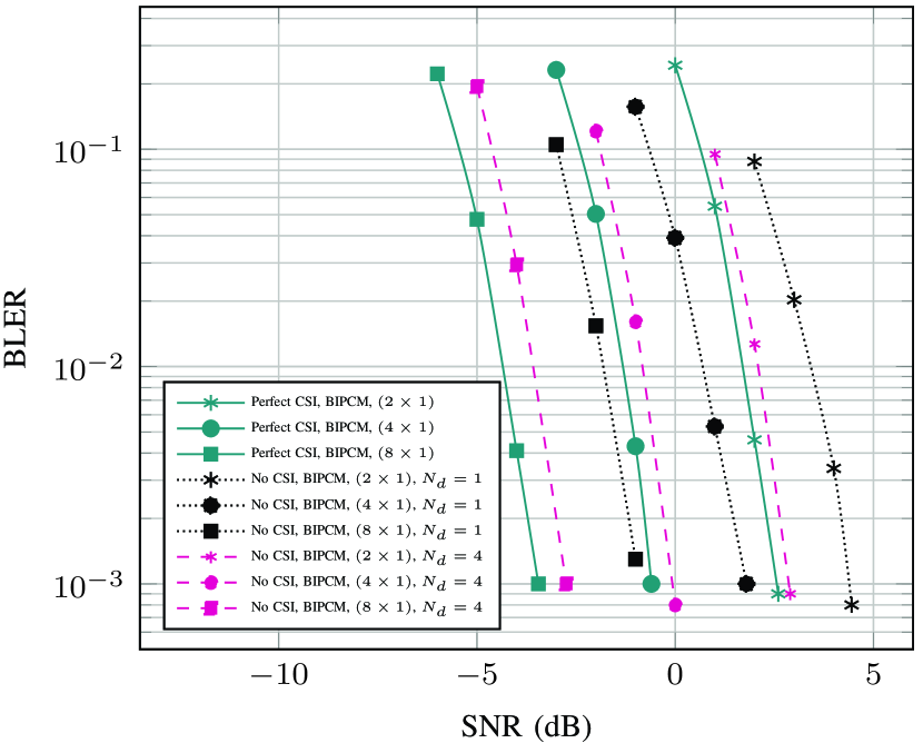
Figure 3: Block Error Rate, 48 bits(TBs+CRC), NRPOLAR BICM, R=48/64, (CRC)-aided successive-cancellation list decoder(List length=8), QPSK modulation, 1 OFDM symbol, 4 PRBs, 48 REs (32 data, 16 DMRS), $N_{T}$=1, $N_{R}=\{2,4,8\}$, $\alpha=1$, LOS channel.

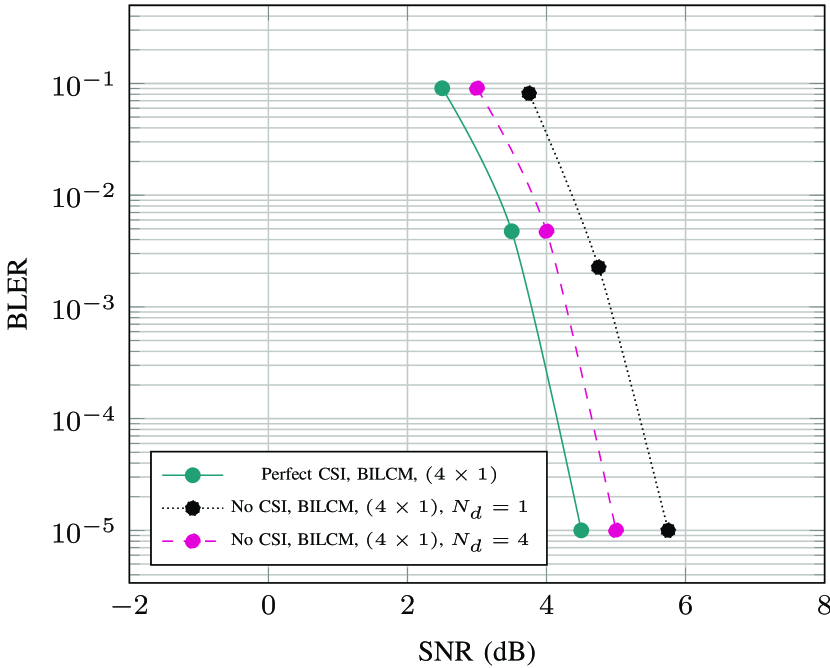
Figure 4: Block Error Rate, 48 bits(TBs+CRC), NRLDPC BICM, R=48/64, Layered belief propagation decoder, iteration=30, QPSK modulation, 1 OFDM symbol, 4 PRBs, 48 REs (32 data, 16 DMRS), $N_{T}$=1, $N_{R}$ = 4, $\alpha=1$, LOS channel.

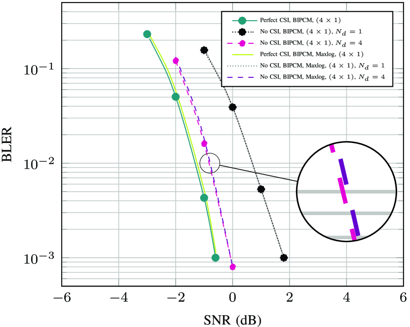
Figure 5: Block Error Rate, 48 bits(TBs+CRC), NRPOLAR BICM, R=48/64, (CRC)-aided successive-cancellation list decoder(List length=8), QPSK modulation, 1 OFDM symbol, 4 PRBs, 48 REs (32 data, 16 DMRS), $N_{T}$=1, $N_{R}$ = 4, $\alpha=1$, LOS channel, Accurate Metric vs Max-log metric.

Note that the $N_{d}=1$ case also refers to the conventional receiver utilizing separate channel estimation. The joint estimation/detection($N_{d}=4$) approach yields a perfomance gain of $1.25$ dB, $1.5$ dB and $1.75$ fB over 2, 4 and 8 receive antennas respectively. From this insight, it is apparent that when the number of antennas increases, the performance gap between the Perfect CSI and the No CSI situations (e.g., $N_{d}=4$) expands. Similarly, the results in Figure 5 using BIPCM are congruent with those presented in Figure 5 that employs BILCM, in both single and multiple antenna configurations. Although the code rates and transmission parameters are identical, BIPCM offers significantly better performance gains than BILCM. This is potentially due to the fact that the 3GPP polar code has been optimized for very short block lengths, while the 3GPP LDPC code targets much longer transport block lengths.

Furthermore, Figure 5 indicate that the max-log metric performs nearly as well as the accurate metric. This leads to the conclusion that when Gray-mapped constellations are employed, the max-log metric is known to have a minimal impact on receiver performance. However, as the modulation order increases, the difference in performance between optimal and suboptimal techniques for generating LLRs becomes significant as discussed in [12]. The logarithmic calculations tied to the precise metric add an extra layer of complexity when incorporating the requisite multiplicative and additive operations during LLR processing.

Finally, we can assess the above results with respect to the finite block length bounds that have been established in the scientific literature [5, 13, 14, 7, 3]. For a more comprehensive understanding of the bounds utilized in Figure 8, interested readers are encouraged to refer to the works of authors [3, 13]. For this purpose, we consider the metaconverse (MC) and Random Coding Union (RCU) bounds for a thorough comparative analysis. It can be observed that when the block error rate (BLER) reaches a threshold of $1\%$, the performance difference between the MC Bound and the No-CSI($N_{d}=4$) is $0.7$ dB, compared to $2.2$ dB for the No-CSI($N_{d}=1$).

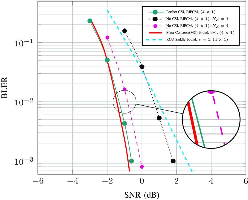
Figure 6: Block Error Rate, 48 bits(TBs+CRC), NR POLAR BICM, R=48/64, (CRC)-aided successive-cancellation list decoder(List length=8), QPSK modulation, 1 OFDM symbol, 4 PRBs, 48 REs (32 data, 16 DMRS), $N_{T}$=1, $N_{R}$ = 4 over LOS channel, vs converse and achievability bounds.

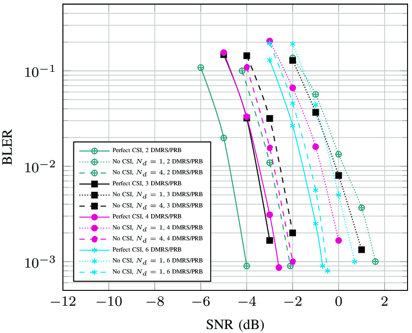
Figure 7: Block Error Rate, 24 bits(TBs), NR POLAR BICM, (CRC)-aided successive-cancellation list decoder, QPSK modulation, 1 OFDM symbol, 4 PRBs, 48 REs, set of ($\{24,32,36,40\}$ data, $\{24,16,12,8\}$ DMRS), $N_{T}$=1, $N_{R}$ = 4, $\alpha=1$, LOS channel.

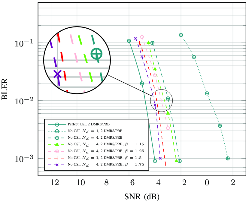
Figure 8: Block Error Rate, 24 bits(TBs), NR POLAR BICM, (CRC)-aided successive-cancellation list decoder, QPSK modulation, 1 OFDM symbol, 4 PRBs, 48 REs, ($40$REs= data, $8$REs= DMRS), $N_{T}$=1, $N_{R}$ = 4, $\alpha=1$, LOS channel, adaptive power adjustment via $\beta$ with $N_{d}=4$ and $N_{d}=1$.

IV-B Impact of DMRS density

In instances where the reference and data symbols are jointly conveyed in common OFDM symbols, we can look into the impact of DMRS density on performance. Figure 8 depicts the performance on the LOS channel in the situations of Perfect CSI and No CSI ($N_{d}=1$, $N_{d}=4$) depending on the density of DMRS per PRB. In essence, fewer DMRS has merit of additional coding rates. Therefore, performance improves as DMRS density decreases. However, it should be noted that even with $N_{d}=4$, a low DMRS density setup expands the performance gap between Perfect CSI and No CSI. It may be advantageous in some instances to maintain the density of DMRSs in a certain sweet spot or simply to rely on sparse or even low DMRS density while increasing their power via an adaptive adjustment. More specifically, a precise approach is to identify the configuration with the minimum number of DMRSs which allows the transmitter to slightly increase the power of the underlying signals. However, choosing a low DMRS density has a detrimental effect on channel estimate quality. Even if the receiver with block detection ($N_{d}=4$) seems to be less sensitive to it with respect to the conventional receiver ($N_{d}=1$). There appears to be a sweet spot in terms of DMRS density per PRB, as evidenced by the results presented in Figure 8. Therefore, the ideal DMRS distribution setup is obtained by incorporating four DMRSs per physical resource block compared to those employing two, three or six DMRSs per PRB , using the block detection principle ($N_{d}=4$). In practice, transmission with a low density of DMRS appears to be more valuable. Consequently, it is advisable to consider configurations with either one or two DMRS per PRB. However in order to reap from the low DMRS density, it is important to carry out some sort of adaptive DMRS/data power adjustment that would enhance the channel estimate accuracy, leading to an improvement in performance from a holistic perspective. For this purpose, the system model can be reconceived as $\mathbf{y}_{i}=\left(\mathbf{x}^{(d)}+\beta\mathbf{x}^{(p)}\right)\mathbf{h}_{i}+\mathbf{z}_{i}$. The adaptive power adjustment procedure is contingent on the values of $\beta$. The DMRS Power is to be slightly increased in a judicious fashion since $\beta$ must be perfectly calibrated to ensure compliance with potential radio frequency constraints.

As depicted in Figure  8, the performance improvement can be observed as a function of varying values of $\beta$. The optimal performance enhancement is achieved when $\beta$ is set to $1.75$. It is noted that by selecting $\beta=1.5$, a gain of $1$ dB can be attained when $N_{d}=4$.

Overall, the implications of varying DMRS density within the 3GPP standard are significant. Specifically, it is feasible to reduce the number of DMRS per PRB to one or two, while allowing the User Equipment (UE) to adjust the power allocation between the DMRS and data transmission. This flexibility in DMRS density and power allocation is transparent to the receiver.

V Conclusions

This paper presented novel bit-interleaved coded modulation metrics for joint estimation detection using a training or reference signal transmission strategy for short to long block length channels. The proposed techniques take advantage of joint estimation/detection. We considered transmissions where reference signals are interleaved with data and both are transmitted over a small number of OFDM symbols so that near-perfect channel estimation cannot be achieved. Our findings demonstrate that BICM metrics combined with the joint estimation/detection principle can be used to achieve detection performance that is close to that of a coherent receiver with perfect channel state information for both polar and LDPC coded configurations. Furthermore, we showed that for transmissions with low DMRS density, a good trade-off can be achieved in terms of additional coding gain and improved channel estimation quality by adaptive DMRS power adjustment.

References

- [1] B. Lee, S. Park, D. J. Love, H. Ji and B. Shim, ”Packet Structure and Receiver Design for Low Latency Wireless Communications With Ultra-Short Packets,” in IEEE Transactions on Communications, vol. 66, no. 2, pp. 796-807, Feb. 2018.
- [2] M. Sy, R. Knopp”Enhanced Low-Complexity Receiver Design for Short Block Transmission Systems,” 34th IEEE International Symposium on Personal, Indoor and Mobile Radio Communications(PIMRC 2023 ), Toronto, ON, Canada, Sept 2023.
- [3] M. Xhemrishi, M. C. Coşkun, G. Liva, J. Östman and G. Durisi, ”List Decoding of Short Codes for Communication over Unknown Fading Channels,” 2019 53rd Asilomar Conference on Signals, Systems, and Computers, Pacific Grove, CA, USA, 2019, pp. 810-814.
- [4] P. Yuan, M. C. Coşkun and G. Kramer, ”Polar-Coded Non-Coherent Communication,” in IEEE Communications Letters, vol. 25, no. 6, pp. 1786-1790, June 2021.
- [5] Y. Polyanskiy, H. V. Poor and S. Verdu, ”Channel Coding Rate in the Finite Blocklength Regime,” in IEEE Transactions on Information Theory, vol. 56, no. 5, pp. 2307-2359, May 2010.
- [6] G. Durisi, T. Koch, J. Östman, Y. Polyanskiy and W. Yang, ”Short-Packet Communications Over Multiple-Antenna Rayleigh-Fading Channels,” in IEEE Transactions on Communications, vol. 64, no. 2, pp. 618-629, Feb. 2016.
- [7] J. Östman, G. Durisi, E. G. Ström, M. C. Coşkun and G. Liva, ”Short Packets Over Block-Memoryless Fading Channels: Pilot-Assisted or Noncoherent Transmission?,” in IEEE Transactions on Communications, vol. 67, no. 2, pp. 1521-1536, Feb. 2019.
- [8] E. Zehavi, “8-PSK trellis codes for a Rayleigh fading channel”,IEEE Transactions on Communication, vol.40, pp. 873–883, 1992, May 1992.
- [9] A. G. i Fàbregas, A Martinez and G. Caire, “Bit-Interleaved Coded Modulation”, Foundations and Trends® in Communications and Information Theory Vol. 5: No. 1–2, pp 1-153, November 2008.
- [10] G. Caire, G. Taricco and E. Biglieri, “ Bit- Interleaved Coded Modulation”, IEEE Transactions on Information Theory, vol. 44, pp. 927–946, May 1998.
- [11] 3GPP TS 38.212 V16.2.0, “ Technical Specification Group Radio Access Network, Multiplexing and channel coding”, July 2020.
- [12] L. Szczecinski, A. Alvarado and R. Feick, ”Closed-form approximation of Coded BER in QAM-based BICM Faded Transmission,” 2008 IEEE Sarnoff Symposium, Princeton, NJ, USA, pp. 1-5, 2008.
- [13] A. Martinez and A. G. i Fàbregas, ”Saddlepoint approximation of random-coding bounds,” 2011 Information Theory and Applications Workshop, La Jolla, CA, USA, 2011, pp. 1-6.
- [14] T. Erseghe, “Coding in the Finite-Blocklength Regime: Bounds Based on Laplace Integrals and Their Asymptotic Approximations,” in IEEE Transactions on Information Theory, vol. 62, no. 12, pp. 6854-6883, Dec. 2016.
- [15] Woodbury, Max A., “Inverting modified matrices”, Statistical Research Group, Memo. Rep. no. 42, Princeton University, Princeton, N. J., 1950. pp.4.
- [16] I. S. Gradshteyn and I. M. Ryzhik, “Table of Integrals, Series and Products” Academic Press, Seventh edition, 2007.